On the Maximum ABC Spectral Radius
of Connected Graphs and Trees

Abstract
Let $G=(V,E)$ be a connected graph, where $V=\{v_{1},v_{2},\cdots,v_{n}\}$ and $m=|E|$. $d_{i}$ will denote the degree of vertex $v_{i}$ of $G$, and $\Delta=\max_{1\leq i\leq n}d_{i}$. The ABC matrix of $G$ is defined as $M(G)=(m_{ij})_{n\times n}$, where $m_{ij}=\sqrt{(d_{i}+d_{j}-2)/(d_{i}d_{j})}$ if $v_{i}v_{j}\in E$, and 0 otherwise. The largest eigenvalue of $M(G)$ is called the ABC spectral radius of $G$, denoted by $\rho_{ABC}(G)$. Recently, this graph invariant has attracted some attentions. We prove that $\rho_{ABC}(G)\leq\sqrt{\Delta+(2m-n+1)/\Delta-2}$. As an application, the unique tree with $n\geq 4$ vertices having second largest ABC spectral radius is determined.

Keywords: ABC matrix, Eigenvalues, ABC spectral radius, Upper bounds, Trees.

1 Introduction

Let $G=(V,E)$ be a simple connected graph. Suppose $V=\{v_{1},v_{2},\cdots,v_{n}\}$ and $m=|E|$. If $c=m-n+1$ ($\geq 0$), then $G$ is called a $c$-cyclic graph. In particular, $G$ is called a tree and a unicyclic graph if $c=1,2$, respectively. As usual, $S_{n}$, $P_{n}$, $C_{n}$, and $K_{n}$ will denote the star, path, cycle, and complete graph with $n$ vertices, respectively.

Let $d_{i}$ denote the degree of vertex $v_{i}$, and $\Delta=\max_{1\leq i\leq n}d_{i}$. The atom-bond connectivity index (ABC index in short) of $G$ is defined [1] as $ABC(G)=\Sigma_{v_{i}v_{j}\in E}f(d_{i},d_{j})$, where $f(x,y)=\sqrt{(x+y-2)/(xy)}$. Since this index can predict well the heat of formation of alkanes (see [2, 3]), it became a hot topic in the past few years (see [4-30]).

In 2017, Estrada [31] defined the ABC matrix of $G$ as $M=M(G)=(m_{ij})_{n\times n}$, where $m_{ij}=f(d_{i},d_{j})$ if $v_{i}v_{j}\in E$, and $0$ otherwise. The chemical background of this matrix was explicated in [31]. The eigenvalues of $M$ are called the ABC eigenvalues of $G$. Because $M$ is non-negative, symmetric, and irreducible, any ABC eigenvalue of $G$ is real. In particular, the largest ABC eigenvalue of $G$ is called its ABC spectral radius, and denoted by $\rho_{ABC}(G)$. Obviously, $\rho_{ABC}(G)$ is positive and simple. Moreover, there exists a unique vector $x>0$ such that $\rho_{ABC}(G)=\max_{\|y\|=1}y^{T}My=x^{T}Mx$, which is known as the Perron vector of $M$.

Estrada [31] proved that $\frac{2}{n}ABC(G)\leq\rho_{ABC}(G)\leq\max_{1\leq i\leq n}M_{i}$, with both equalities iff $M_{1}=M_{2}=\cdots=M_{n}$, where $M_{i}=\sum_{1\leq j\leq n}m_{ij}$. Recently, Chen [32] presented another lower bound of $\rho_{ABC}(G)$ in terms of $R_{-1}(G)$, which is the sum of $\frac{1}{d_{i}d_{j}}$ over all edges $v_{i}v_{j}\in E$. Chen [32] further proposed the problem of characterizing graphs with extremal ABC spectral radius for a given graph class. Soon, this problem for trees, connected graphs, and unicyclic graphs were solved by Chen [33], Ghorbani et al. [34], and Li et al. [35], respectively.

Lemma 1.1 [33]. Let $T$ be a tree with $n\geq 3$ vertices. Then

$$\sqrt{2}\cos\frac{\pi}{n+1}\leq\rho_{ABC}(G)\leq\sqrt{2n-4},$$

with left (right) equality iff $G\cong P_{n}$ (resp. $G\cong S_{n}$).

Lemma 1.2 [34] . Let $G$ be a connected graph with $n\geq 3$ vertices. Then

$$\sqrt{2}\cos{\frac{\pi}{n+1}\leq\rho_{ABC}(G)\leq\sqrt{2n-4}},$$

with the left (right) equality iff $G\cong P_{n}$ (resp. $G\cong K_{n}$ ).

Lemma 1.3 [35] . Let $G$ be a unicyclic graph with $n\geq 4$ vertices. Then

$$\sqrt{2}\ =\rho_{ABC}(C_{n})\leq\rho_{ABC}(G)\leq\rho_{ABC}(S_{n}+e),$$

with the left (right) equality iff $G\cong C_{n}$ (resp. $G\cong S_{n}+e$).

For convenience, let $\mathcal{C}(n)$ be the set of connected graphs with $n$ vertices, and $\mathcal{G}(m,n)$ the set of connected graphs with $n$ vertices and $m$ edges. In the present paper, we consider upper bounds of $\rho_{ABC}$ for connected graphs. In Section 2, it is shown that, if $G\in\mathcal{G}(m,n)$ and $\Delta(G)=\Delta$, then $\rho_{ABC}(G)\leq\sqrt{\Delta+(2m-n+1)/\Delta-2}$. As an application, in Section 3, we characterize the unique tree with $n\geq 4$ vertices having the second largest ABC spectral radius. Finally, some problems are proposed in Section 4.

2 Some upper bounds of the ABC spectral radius

In this section, we present two upper bounds of $\rho_{ABC}$ of connected graphs.

Theorem 2.1. If $G\in\mathcal{G}(m,n)$ and $\Delta(G)=\Delta$, then

$$\rho_{ABC}(G)\leq\sqrt{\Delta+(2m-n+1)/\Delta-2}.$$

Moreover, the bound is attainable.

Proof. Let $M=M(G)$, $D=2m-n+1$, and $x=(\sqrt{d_{1}},\sqrt{d_{2}},\cdots,\sqrt{d_{n}})^{T}$. From the Perron-Frobenius theory, it suffices to confirm the claim: $(Mx)_{i}\leq\sqrt{d_{i}}\sqrt{\Delta+D/\Delta-2}$ or $[(Mx)_{i}/\sqrt{d_{i}}]^{2}\leq\Delta+D/\Delta-2$ holds for $1\leq i\leq n$.

If $d_{i}<D/\Delta$, then $(Mx)_{i}=\sum\limits_{v_{i}v_{j}\in E}f(d_{i},d_{j})\sqrt{d_{j}}\leq d_{i}\sqrt{\frac{d_{i}+\Delta-2}{d_{i}}}<\sqrt{d_{i}}\sqrt{D/\Delta+\Delta-2}$. Hence assume $d_{i}\geq D/\Delta$. By using the Cauchy-Schwarz Inequality we have

$$(Mx)_{i} =\sum\limits_{v_{i}v_{j}\in E}\sqrt{(d_{i}+d_{j}-2)/d_{i}}$$

$$\leq\sqrt{d_{i}^{2}-2d_{i}+\sum\limits_{v_{i}v_{j}\in E}d_{j}}$$

$$\leq\sqrt{d_{i}^{2}-2d_{i}+[2m-d_{i}-(n-d_{i}-1)]}$$

$$=\sqrt{d_{i}^{2}-2d_{i}+D}.$$

Thus we have $[(Mx)_{i}/\sqrt{d_{i}}]^{2}\leq(d_{i}^{2}-2d_{i}+D)/d_{i}=d_{i}+D/d_{i}-2$. Since $\eta(x)=x+D/x-2$ is a Nike function and $D/\Delta\leq d_{i}\leq\Delta$, it follows that

$$[(Mx)_{i}/\sqrt{d_{i}}]^{2}\leq\max\{\eta(D/\Delta),\eta(\Delta)\}=\Delta+D/\Delta-2.$$

Finally, to see the bound is attainable, one can take $S_{n}$ and $K_{n}$ as examples. The proof is thus completed. $\blacksquare$

Let $\theta(m,\Delta)=\sqrt{\Delta+(2m-n+1)/\Delta-2}$. For fixed $m$, the monotonicity of $\theta$ with respect to $\Delta$ is clear. Hence Theorem 2.1 can easily produce a upper bound of $\rho_{ABC}$ for subsets of $\mathcal{G}(m,n)$. For example, an upper bound for $c$-cyclic graphs is obtained as follows.

Corollary 2.2. Let $G$ be a $c$-cyclic graph with $n\geq 3$ vertices, and $c\leq(n-1)/2$. Then

$$\rho_{ABC}(G)\leq\sqrt{n-2+2c/(n-1)}.$$

Proof. Since $m=n-1+c$ and $c\leq(n-1)/2$, by direct calculations we have

$$\theta(m,2)=\sqrt{(n-1)/2+c}\leq\theta(m,n-1)=\sqrt{n-2+2c/(n-1)},$$

and the conclusion follows from Theorem 2.1. $\blacksquare$

It is easily seen that, Theorem 2.1 can reproduce the upper bound part of Lemma 1.1. However, if we consider upper bounds of $\rho_{ABC}$ for a subset of $\mathcal{C}_{n}$, whose elements have various sizes (numbers of edges), Theorem 2.1 may be not so convenient to applied directly. Hence we deduce the following result.

Corollary 2.3. If $G\in\mathcal{G}(m,n)$ and $\Delta(G)=\Delta$, then $\rho_{ABC}(G)\leq\sqrt{\Delta+k-2}$, where $k=\lceil(2m-n+1)/\Delta\rceil$.

Proof. From $k=\lceil(2m-n+1)/\Delta\rceil\geq(2m-n+1)/\Delta$, the conclusion holds immediately from Theorem 2.1. $\blacksquare$

Though Corollary 2.3 is weaker than Theorem 2.1, the upper bound $\theta^{\prime}(m,\Delta)=\sqrt{\Delta+k-2}$ has better property than $\theta(m,\Delta)$. In fact, for fixed $m$, $\theta^{\prime}(m,\Delta)$ almost strictly decreases with $\Delta$. To see this, let $\Delta_{1}>\Delta_{2}$ and $D=2m-n+1$. We illustrate the fact with the following two cases.

Case 1. $D/k\leq\Delta_{2}<\Delta_{1}<D/(k-1)$. Then $\theta^{\prime}(m,\Delta_{2})<\theta^{\prime}(m,\Delta_{1})$ obviously.

Case 2. $D/k\leq\Delta_{2}<D/(k-1)\leq\Delta_{1}$. Then

$$\theta^{\prime}(m,\Delta_{2}) =\sqrt{\Delta_{2}+k-2}$$

$$\leq\sqrt{\Delta_{1}+k-3}$$

$$=\theta^{\prime}(m,\Delta_{1}),$$

with equality iff $\Delta_{2}=D/(k-1)-1=\Delta_{1}-1$.

By the monotonicity of $\theta^{\prime}(m,\Delta)$ with respect to $\Delta$, we are able to reproduce the upper bound part of Lemma 1.2.

Corollary 2.4 [34] . Let $G$ be a connected graph with $n\geq 3$ vertices. Then

$$\rho_{ABC}(G)\leq\sqrt{2n-4},$$

with equality iff $G\cong K_{n}$.

Proof. By the monotonicity of $\theta^{\prime}$ we have $\theta^{\prime}(m,\Delta)\leq\theta^{\prime}(m,n-1)\leq\theta^{\prime}(n(n-1)/2,n-1)$, with all the equalities iff $m=n(n-1)/2$, that is, $G\cong K_{n}$. The conclusion thus follows from Corollary 2.3. $\blacksquare$

3 The tree with second largest ABC spectral radius

In order to further illustrate the application of Theorem 2.1 and Corollary 2.3, in this section we determine the tree with $n\geq 4$ vertices, whose ABC spectral radius is the second largest. For convenience, let $\mathcal{T}_{n}$ be the set of trees with $n$ vertices, and $\mathcal{T}_{n}^{(\Delta)}=\{T\in\mathcal{T}_{n}|\Delta(T)=\Delta\}$. Let $T_{i}$, $i=1,2,3,4$, be the trees shown in Figure 1. $T_{1}$ is just the double star $S_{n-3,1}$. If $T\in\mathcal{T}_{n}^{(\Delta)}$, then $T$ contains $S_{\Delta+1}$ as its (induced) subgraph, hence it is easily seen that $\mathcal{T}_{n}^{(n-1)}=\{S_{n}\}$, $\mathcal{T}_{n}^{(n-2)}=\{S_{n-3,1}\}$, and $\mathcal{T}_{n}^{(n-3)}=\{T_{2},T_{3},T_{4}\}$.

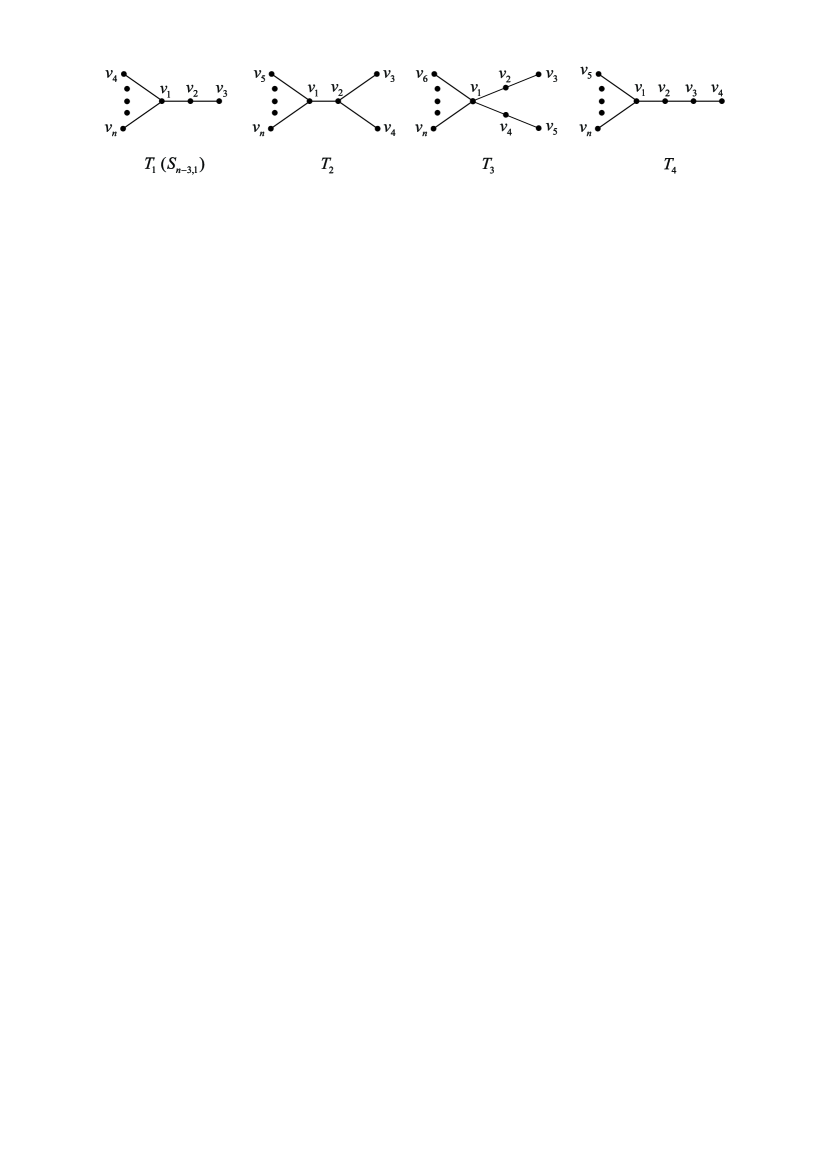
Figure 1: The trees $T_{i}$, i=1, 2, 3, 4.

Our aim in this section is to prove the following conclusion.

Theorem 3.1. If $n\geq 4$ and $T\in\mathcal{T}_{n}-\{S_{n},S_{n-3,1}\}$, then

$$\rho_{ABC}(T)<\rho_{ABC}(S_{n-3,1})<\rho_{ABC}(S_{n}).$$

We need some more preliminaries before presenting the proof of Theorem 3.1.

For two vertices $u$ and $v$ of a graph $G$, they are said to be equivalent, denoted by $u\sim v$, if there is an automorphism of $G$ sending $u$ to $v$. By symmetry, the following result is immediate.

Lemma 3.2. Let $x$ be the Perron vector of the ABC matrix $M(G)$ of a connected graph $G$. If $u\sim v$, then $x_{i}=x_{j}$.

Lemma 3.3. $\rho_{ABC}(S_{n-3,1})>\sqrt{n-3.5}$ if $n\geq 4$.

Proof. Let $\rho=\rho_{ABC}(S_{n-3,1})$, and label the vertices of $S_{n-3,1}$ as in Figure 1. Based on Lemma 3.2, let $x=(x_{1},x_{2},x_{3},x_{4},\cdots,x_{4})^{T}$ be the Perron vector of $M=M(S_{n-3,1})$. From $\rho x=Mx$ we have

$$\left\{\begin{aligned} &\rho x_{1}=(n-3)\sqrt{\frac{n-3}{n-2}}x_{4}+\sqrt{\frac{1}{2}}x_{2}\\ &\rho x_{2}=\sqrt{\frac{1}{2}}x_{1}+\sqrt{\frac{1}{2}}x_{3}>\sqrt{\frac{1}{2}}x_{1}\\ &\rho x_{4}=\sqrt{\frac{n-3}{n-2}}x_{1}\end{aligned}\right..$$

Hence $\rho^{2}x_{1}=(n-3)\sqrt{\frac{n-3}{n-2}}\rho x_{4}+\sqrt{\frac{1}{2}}\rho x_{2}>\frac{(n-3)^{2}}{n-2}x_{1}+\frac{1}{2}x_{1}$, and we arrive at

$$\rho^{2}>\frac{(n-3)^{2}}{n-2}+\frac{1}{2}>n-4+0.5=n-3.5,$$

which completes the proof. $\blacksquare$

Lemma 3.4. If $n\geq 6$ and $T\in\{T_{2},T_{3},T_{4}\}$, then $\rho_{ABC}(T)<\sqrt{n-3.5}$.

Proof. If $n=6$, the conclusion can be verified easily. Hence assume $n\geq 7$. Label the vertices of $T$ as in Figure 1. Let $M=M(T)$ and $x=(\sqrt{d_{1}},\sqrt{d_{2}},\cdots,\sqrt{d_{n}})^{T}$. Based on Lemma 2.1, we prove the result by confirming $(Mx)_{i}/\sqrt{d_{i}}\leq\sqrt{n-3.5}$ for $1\leq i\leq n$.

We have $(Mx)_{i}/\sqrt{d_{i}}\leq\sqrt{d_{i}-2+\sum_{v_{i}v_{j}\in E}d_{j}/d_{i}}$ from the proof of Theorem 2.1. Hence $(Mx)_{1}/\sqrt{d_{1}}\leq\sqrt{n-5+(n-1)/(n-3)}=\sqrt{n-4+2/(n-3)}\leq\sqrt{n-3.5}$. For $i\geq 2$, because $d_{i}\leq 3$ and $n\geq 7$, it follows

$$(Mx)_{i}/\sqrt{d_{i}}\leq\max\{\sqrt{n-4},\sqrt{(n-1)/2},\sqrt{(n+2)/3}\}<\sqrt{n-3.5},$$

and the proof is completed. $\blacksquare$

Now we present the proof of Theorem 3.1.

Proof of Theorem 3.1. It is easily seen that $\mathcal{T}_{4}=\{S_{4},S_{1,1}\cong P_{4}\}$, $\mathcal{T}_{5}=\{S_{5},S_{2,1},P_{5}\}$, and $\mathcal{T}_{6}=\{S_{6},S_{3,1},T_{2},T_{3},T_{4},P_{6}\}$, so the conclusion holds if $n\leq 6$ from Lemmas 1.1, 3.3, and 3.4. Hence assume $n\geq 7$.

If $\Delta\geq n-3$, the conclusion follows from Lemmas 3.3 and 3.4. Otherwise, if $\Delta\leq n-4$, then $\rho_{ABC}(T)\leq\theta^{\prime}(n-1,n-4)=\sqrt{n-6+\lceil(n-1)/(n-4)\rceil}\leq\sqrt{n-4}$ from Corollary 2.3.

The proof is thus completed. $\blacksquare$

4 Further discussions

In this paper, it is shown that $\rho_{ABC}(G)\leq\sqrt{\Delta+(2m-n+1)/\Delta-2}$ if $G\in\mathcal{G}(m,n)$ and $\Delta(G)=\Delta$. The bound is attained by $S_{n}$ and $K_{n}$. Firstly, the following problem may be worth consideration.

Problem 4.1. Characterize the graphs $G\in\mathcal{G}(m,n)$ such that

$$\rho_{ABC}(G)=\sqrt{\Delta(G)+(2m-n+1)/\Delta(G)-2}.$$

As well, the double star $S_{n-3,1}$ is shown to be the unique tree having second largest ABC spectral radius in $\mathcal{T}_{n}$, $n\geq 4$. Recall that, Lin et al. [36] ordered trees by their (adjacent) spectral radius $\lambda_{1}$, and showed that, if $T_{1}$ and $T_{2}$ are two trees with $n\geq 4$ vertice and $\Delta(T_{1})>\Delta(T_{2})\geq(2n)/3-1$, then $\lambda_{1}(T_{1})>\lambda_{1}(T_{2})$. Naturally, the following question is interesting.

Question 4.2. Let $G_{1}$ and $G_{2}$ be two graphs in a subset of $\mathcal{G}(m,n)$. Is there some integer $l(m,n)$ (depending on $n$ and/or $m$), such that if $\Delta(G_{1})>\Delta(G_{2})\geq l(m,n)$, then $\rho_{ABC}(G_{1})>\rho_{ABC}(G_{2})$?

This question may be difficult to answer at the present, even for trees, and the following two problems are worth investigation in advance.

Problem 4.3 Order graphs in some classes of connected graphs by their ABC spectral radii.

Problem 4.4. Establish non-trivial lower bounds of $\rho_{ABC}(G)$ for a graph $G\in\mathcal{G}(m,n)$ (in terms of $m$, $n$, and $\Delta(G))$.

References

• [1] E. Estrada, L. Torres, L. RodrΓ­guez, I. Gutman, An atom-bond connectivity index: Modelling the enthalpy of formation of alkanes, Indian J. Chem. 37A (1998) 849-855.
• [2] E. Estrada, Atom-bond connectivity and the energetic of branched alkanes, Chem. Phys. Lett. 463 (2008) 422-425.
• [3] I. Gutman, J. ToΕ‘oviΔ‡, S. RadenkoviΔ‡, S. MarkoviΔ‡, On atom-bond connectivity index and its chemical applicability, Indian J. Chem. 51A (2012) 690-694.
• [4] B. Furtula, A. Graovac, D. VukičeviΔ‡, Atom-bond connectivity index of trees, Discr. Appl. Math. 157 (2009) 2828-2835.
• [5] K. C. Das, Atom-bond connectivity index of graphs, Discr. Appl. Math. 158 (2010) 1181-1188.
• [6] R. Xing, B. Zhou, Z. Du, Further results on atom-bond connectivity index of trees, Discr. Appl. Math. 157 (2010) 1536-1545.
• [7] R. Xing, B. Zhou, F. Dong, On atom-bond connectivity index of connected graphs, Discr. Appl. Math. 159 (2011) 1617-1630.
• [8] J. Chen, X. Guo, Extreme atom-bond connectivity index of graphs, MATCH Commun. Math Comput. Chem. 65 (2011) 713-722.
• [9] K. C. Das, I. Gutman, B. Furtula, On atom-bond connectivity index, Chem. Phys. Lett. 511 (2011) 452-454.
• [10] J. Chen, J. Liu, X. Guo, Some upper bounds for the atom-bond connectivity index of graphs, Appl. Math. Lett. 25 (2012) 1077-1081.
• [11] I. Gutman, B. Furtula, M. IvanoviΔ‡, Notes on trees with minimal atom-bond connectivity index, MATCH Commun. Math Comput. Chem. 67 (2012) 467-482.
• [12] W. Lin, T. Gao, Q. Chen, X. Lin, On the atom-bond connectivity index of connected graphs with a given degree sequence, MATCH Commun. Math. Comput. Chem. 69 (2013) 571-578.
• [13] W. Lin, X. Lin, T. Gao, X. Wu, Proving a conjecture of Gutman concerning trees with minimal ABC index, MATCH Commun. Math. Comput. Chem. 69 (2013) 549-557.
• [14] I. Gutman, B. Furtula, M. B. Ahmadi, S. A. Hosseini, P. Salehi Nowbandegani, M. Zarrinderakht, The ABC index conundrum, Filomat 27 (2013) 1075-1083.
• [15] D. Dimitrov, On structural properties of trees with minimal atom-bond connectivity index, Discr. Appl. Math. 172 (2014) 28-44.
• [16] D. Dimitrov, On structural properties of trees with minimal atom-bond connectivity index II: Bounds on $B_{1}$- and $B_{2}$-branches, Discr. Appl. Math. 204 (2016) 90-116.
• [17] Z. Du, C. M. da Fonseca, On a family of trees with minimal atom-bond connectivity index, Discr. Appl. Math. 202 (2016) 37-49.
• [18] D. Dimitrov, Z. Du, C. M. da Fonseca, On structural properties of trees with minimal atom-bond connectivity index III: Trees with pendent paths of length three, Appl. Math. Comput. 282 (2016) 276-290.
• [19] D. Dimitrov, On structural properties of trees with minimal atom-bond connectivity index IV: Solving a conjecture about the pendent paths of length three, Appl. Math. Comput. 313 (2017) 418-430.
• [20] D. Dimitrov, Z. Du, C. M. da Fonseca, Some forbidden combinations of branches in minimal-ABC trees, Discr. Appl. Math. 236 (2018) 165-182.
• [21] K. C. Das, S. Elumalai, I. Gutman, On ABC index of graphs, MATCH Commun. Math. Comput. Chem. 78 (2017) 459-468.
• [22] D. Dimitrov, Efficient computation of trees with minimal atom-bond connectivity index, Appl. Math. Comput. 224 (2013) 663-670.
• [23] W. Lin, J. Chen, Q. Chen, T. Gao, X. Lin, B. Cai, Fast computer search for trees with minimal ABC index based on tree degree sequences, MATCH Commun. Math. Comput. Chem. 72 (2014) 699-708.
• [24] W. Lin, C. Ma, Q. Chen, J. Chen, T. Gao, B. Cai, Parallel search trees with minima6l ABC index with MPI + OpenMP, MATCH Commun. Math. Comput. Chem. 73 (2015) 337-343.
• [25] D. Dimitrov, N. MilosavljeviΔ‡, Efficient computation of trees with minimal atom-bond connectivity index revisited, MATCH Commun. Math. Comput. Chem. 79 (2018) 431-450.
• [26] W. Lin, J. Chen, Z. Wu, D. Dimitrov, L. Huang, Computer search for large trees with minimal ABC index, Appl. Math. Comput. 338 (2018) 221-230.
• [27] D. Dimitrov, Z. Du, C. M. da Fonseca, The minimal-ABC trees with $B_{1}$-branches, PLoS ONE 13(4): e0195153. https://doi.org/10.1371/journal.pone.0195153.
• [28] Z. Du, D. Dimitrov, The minimal-ABC trees with $B_{1}$-branches II, IEEE Access 6 (2018) 66350-66366.
• [29] Y. Zheng, W. Lin, Q. Chen, L. Huang, Z. Wu, Characterizing trees with minimal ABC index with computer search: A short survey, J. Discret. Appl. Math. 1 (2018) 1-9.
• [30] Z. Du, D. Dimitrov, The minimal-ABC trees with $B_{2}$-branches, Comp. Appl. Math. 39, 85 (2020). https://doi.org/10.1007/s40314-020-1119-7.
• [31] E. Estrada, The ABC matrix, J. Math. Chem. 55 (2017) 1021 C1033.
• [32] X. Chen, On ABC eigenvalues and ABC energy, Linear Algebra Appl. 544 (2018) 141-157.
• [33] X. Chen, On extremality of ABC spectral radius of a tree, Linear Algebra Appl. 564 (2019) 159-169.
• [34] M. Ghorbania, X. Li, M. Hakimi-Nezhaada, J. Wang, Bounds on the ABC spectral radius and ABC energy of graphs, Linear Algebra Appl. 598 (2020) 145-164.
• [35] X. Li, J. Wang, On the ABC spectra radius of unicyclic graphs, Linear Algebra Appl. 596 (2020) 71-81.
• [36] W. Lin, X. Guo, Ordering trees by their largest eigenvalues, Linear Algebra Appl. 418 (2006) 450-456.