Approximate Inverse Reinforcement Learning from Vision-based Imitation Learning

Abstract

In this work, we present a method for obtaining an implicit objective function for vision-based navigation. The proposed methodology relies on Imitation Learning, Model Predictive Control (MPC), and an interpretation technique used in Deep Neural Networks. We use Imitation Learning as a means to do Inverse Reinforcement Learning in order to create an approximate cost function generator for a visual navigation challenge. The resulting cost function, the costmap, is used in conjunction with MPC for real-time control and outperforms other state-of-the-art costmap generators in novel environments. The proposed process allows for simple training and robustness to out-of-sample data. We apply our method to the task of vision-based autonomous driving in multiple real and simulated environments and show its generalizability.
Supplementary video: https://youtu.be/WyJfT5lc0aQ

I INTRODUCTION

In robotics, vision-based control has become a popular topic as it allows navigating in a variety of environments. A notable contribution is the ability to work in areas where positional information from satellites or motion capture systems is not possible to obtain. While vision-based controls are harder to analytically write equations for when compared to positional-based controls, it has been shown to work by millions of humans using it every day.

Using deep neural networks (NNs) for vision-based control has become ubiquitous in literature thanks to the power of deep learning. However, in general, most of the NN models suffer from the generalization problem or the covariate shift; a trained NN model does not work well on a new test dataset if the distribution of input variables from training and testing dataset are very different from each other.

To solve this generalization problem in new environments, in this work, we focus on generalizing vision-based control systems to new previously unseen environments. This will focus on the ability of a single network to generate reasonable cost functions even in a novel environment not seen during training. We propose an automatic way to generate the grid map cost function, the costmap, without requiring access to a pre-defined costmap or any labels with which to perform segmentation, classification, or recognition. The key idea is using a vision-based end-to-end (E2E) Imitation Learning (IL) framework [1]. In this E2E control approach, we only need to query the expert’s action to learn a costmap of a specific task. During training, the model learns a mapping from sensor input to the control output. Specifically in vision-based autonomous driving, if we train a Deep Neural Network (DNN) by imitation learning and analyze an intermediate layer of Convolutional Neural Networks by reading the activated neurons of the trained network, we see the mapping converged to extracting important features that link the input and the output.

In a broad sense, the convolutional layer parts of the trained E2E network become a function that extracts important features in the input scene. This can be viewed as an implicit image segmentation done inside the deep CNN where the extracted features will depend on the task at hand. For example, if the task is learning to visually track an object, the network will implicitly find the object as an important feature. In another case, if the task is to perform autonomous lane-keeping, the boundaries of the lane will become important for making a final decision.

Our work is obtaining a costmap based on an intermediate convolutional layer activation, but the middle layer output is not directly trained to predict a costmap; instead, it is generating an implicit objective function related to relevant features, which links the input and the output. This allows our work to produce a reasonable costmap on unseen data where direct costmap prediction methods [2] would fail because the data would be out of their prediction domain.

Monocular vision-based planning has shown a lot of success performing visual servoing in ground vehicles [3, 4, 2], manipulators [5], and aerial vehicles [6, 7]. In the autonomous driving literature, [4] learned to generate a costmap from camera images for the Model Predictive Control (MPC) controller. [2] tried to generalize this approach by using a Convolutional LSTM (Conv-LSTM) and a softmax attention mechanism and shows this method working on previously unseen tracks. However, the training of this architecture requires having a predetermined costmap to imitate and the track it was shown to generalize had visually similar components (dirt track and black track borders) to recognize.

End-to-end learning in autonomous driving has been shown to work in various lane-keeping applications [8, 9] and [1] showed great performance by learning both steering and throttle but did not show its generalizability except for different lighting conditions.

[10] proposed an image-space approach for vision-based navigation. The approach plans a path for a ground-based robot in the image-space of an onboard monocular camera. This technique is most related to our approach since they applied a learned color-to-cost mapping to transform a raw image into a costmap-like image, and performed path planning directly in the image space. The limitation of [10] is that they require another supervised learning step to train a model to output the costmap like in [2], whereas our method does not need one. Therefore, our approach is more efficient in learning a costmap without having a prior on what the costmap should look like.

The contributions of this work are threefold:

1. We introduce a novel inverse reinforcement learning method Approximate Inverse Reinforcement Learning (AIRL) which approximates a cost function from an intermediate layer of an end-to-end policy trained with imitation learning.

2. We perform a sampling-based stochastic optimal control, MPPI, in image space, which is perfectly suitable for our driver-view binary costmap.

3. Compared to state-of-the-art methods, the Attention-based Costmap Prediction (ACP) and the end-to-end Imitation Learning (E2EIL), our proposed method is shown to generalize well by generating usable costmaps in environments outside of its training data.

II BACKGROUND

II-A Inverse Reinforcement Learning

In Reinforcement Learning (RL), given that an agent is able to query the reward of applying any action at any state, the goal is to find the optimal policy that maximizes the expected future reward. In Inverse Reinforcement Learning (IRL), the underlying reward function is unknown and the goal is to find the reward function that explains the given optimal policy. IRL can be considered a harder problem to solve than RL, because generally, there is no single reward function that can describe an expert behavior [11].

If we can approximate a reward function from observations, we can then train new agents to maximize this reward. It can be considered similar to Imitation Learning in that sense, as we could train agents to perform according to an expert behavior. However, it is important to note that, unlike in IL, the learning agents could then potentially outperform the expert behavior. This is especially true when the expert behavior is suboptimal or applied in a different environment.

Most of the IRL work in the literature requires one more pipeline of training to figure out the mapping between the input trajectories and the reward function. For example, [12] introduced maximum likelihood approach to IRL while the maximum entropy approach was introduced in [13] to find a generative model that yields trajectories that are similar to the expert’s. They find a weighted distribution of reward basis functions in an iterative way. This step still requires some hand-tuning; for example, picking proper basis functions to form the distribution.

However, in our work, we do not need any new design of basis functions because we learn a policy end-to-end and can get an approximate the reward function for ‘free’, i.e. without any hand-tuning. Since optimal controllers can be considered as a form of model-based RL, the negative of this reward function can then be used as the cost function that our MPC controller optimizes with respect to.

II-B Imitation Learning

In ILs (IL), a policy is trained to accomplish a specific task by mimicking an expert’s control policy, which in most cases, is assumed to be optimal. In this work of perceptual control, we will use sections of a network trained with end-to-end Imitation Learning (E2EIL) using MPC as the expert policy. Literally, E2EIL trains agents to directly output optimal control actions given image data from cameras; end (sensor reading) to end (control).

While IL provides benefits in terms of sample efficiency, it does have drawbacks. Here, we shortly talk about three major problems in IL.

i) Generalizability: Even with online data aggregation methods [14], it is impossible to collect all kinds of unexpected scenarios and edge cases. Accordingly, E2EIL is vulnerable to out-of-training-data (covariate shift) as shown in the literature [15, 16, 17]. There are little to no guarantees on what a Neural Network (NN) trained with IL will output when given an input vastly different from its training set.

ii) Upper-bounded: The best job a learner can do is capped by the ability of a teacher since the objective of the IL setting is to mimic the expert’s behavior.

iii) Interpretability: Since the end-to-end approach uses a totally blackbox model from sensor input to control output, it loses interpretability; when it fails, it is hard to tell if it comes from noise in the input, if the input is different from the training data, or if the model has just chosen a wrong control output due to ending training prematurely.

From these reasons, E2E IL controllers are not widely used in real-world applications, such as self-driving cars. Our approach provides solutions to these problems by leveraging the idea of using Deep Learning (DL) only in some blocks of autonomy, hence becomes more interpretable.

In the case of autonomous driving, given a cost function to optimize and a vehicle dynamics model, we can do path planning and compute an optimal solution via an optimal model predictive controller. Therefore, the problem simplifies from computing a good action to computing a good approximation of the cost function in new environments.

In this paper, we provide evidence of better performance than the expert teacher by showing a higher success rate of task completion when a task requires generalization to new environments.

III MPPI IN IMAGE SPACE

We used a stochastic MPC optimal controller, Model Predictive Path Integral control (MPPI) [18], as an expert in IL and also as an optimal controller for testing our costmap, like in [3, 4, 2]. The details of the MPPI algorithm can be found in multiple literature [19, 18] and here we concisely describe MPPI; MPPI is a sampling-based stochastic optimal controller which can operate on nonlinear dynamics and can have non-convex cost functions. It is an iterative optimization algorithm for path planning and control with a receding time horizon MPC.

For the navigation task, our cost function for the optimal control problem will follow a similar format as in [2] with the squared cost on the desired speed. The cost function at time $t$, which does not penalize the control, is shown as:

$$l(\textbf{x}_{t})=C_{speed}(v_{x}^{d}-v_{x,t})^{2}+C_{crach}I(\textbf{x}_{t}),$$ (1)

where $C_{speed},C_{crash}$ are coefficients that represent the penalty applied for speed and crash, respectively. $I$ is an indicator function that returns $1$ if the vehicle position in the image space is on the high-cost region, and returns $0$ otherwise. $v_{x}$ and $v_{x}^{d}$ are measured body velocity in the $x$ direction and desired velocity respectively. It is important to note that in our settings, near-perfect state estimation and a GPS-track-map is provided when MPPI is used as the expert during data collection, but as in [2], only body velocity, roll, and yaw from the state estimate is used when it is operating using vision at testing. For our navigation task, we followed the same definition of the system state and control in the MPPI paper [18] and [2]: $\mathbf{x}=[x,y,yaw,roll,v_{x},v_{y},\dot{yaw}]$ is the vehicle state in a world coordinate frame and $\mathbf{u}$ is $[throttle,steering]$.

Image space from a mounted camera on a robot is a local and fixed frame; i.e. the state represented in the image space is relative to the robot’s camera. Since we are planning an optimal path given a costmap image in first-person-view, the vehicle’s future state trajectory described in the world coordinates must be transformed into a 2D image in a moving frame of reference. This traditional coordinate transformation technique is widely used in 3D computer graphics [20].

Through the coordinate transform at every timestep, the MPPI-planned final future state trajectory mapped in image space on our costmap looks like Figure 1c.

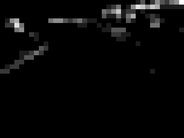
(a) The original output from the deep CNN middle layer. The white colored pixels are the activated neurons averaged among the convolution filters.

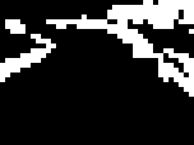
(b) After applying a binary filter. The black and white background represents the costmap that MPPI is optimizing.

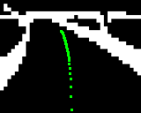
(c) MPPI in image space. The green trajectory is the MPPI-planned future state trajectory in image space.

Figure 1: Running MPPI on image space with the generated costmap.

The crash cost depends on the costmap and it is a binary grid map (0, 1) describing occupancy of features we want to avoid driving through, e.g. track boundaries or lane boundaries on the road.

IV METHODOLOGIES

In this work, we introduce a method for an inverse reinforcement learning problem with the task of vision-based autonomous driving. More specifically, we focus on lane-keeping and collision checking like in [3, 4, 2, 1, 8]. The following methods are evaluated in Section V.

IV-A End-to-End Imitation Learning [1]

[1] constructed a CNN that takes in RGB images and spits out control actions of throttle and steering angles for an autonomous vehicle. It was trained using Data Aggregation (DAgger) algorithm [14] on data provided by an expert MPC controller. While it can achieve aggressive driving targets and was shown to handle various lighting conditions on the same track, it in general does not generalize to brand new tracks. This is most likely due to the images creating a feature space not seen in training. While the last layers may not be able to choose the proper action, intermediate layers still perform some feature extraction. This feature extraction is further discussed in Section IV-C.

IV-B Attention-based Costmap Prediction [2]

The concise description of [2], we call Attention-based Costmap Prediction (ACP), is to create a NN that can take in camera images and output a costmap used by a MPC controller, MPPI. By separating the perception and low-level control into two robust components, this system can be more resilient to small errors in either. Their final model is trained on a mixture of real datasets of a simple racetrack as well as simulation datasets from a more complex track. The full system is then able to drive around the real-world version of the complex track in an aggressive fashion without crashing. It is the most generalized method for achieving autonomous driving in new environments that the authors of this paper have found in the literature.

IV-C Approximate Inverse Reinforcement Learning (ours)

Our method can be considered a mixture of the two previously mentioned; we will be using both E2EIL and an MPC controller. Although our work relies on E2EIL and MPC, we tackle a totally different problem: IRL from E2EIL. Our main contribution is learning an approximate, ‘generalizable’ costmap ‘from’ E2EIL. On top of this AIRL, we perform MPC in image space (Section III) with a real-time-generated agent-view costmap. The reason why we named it ‘Approximate’ IRL is because we do not directly train a model to output a cost function.

To support our method, we borrow the ideas from one of the interpretation techniques used for interpreting the information flow inside DNNs. Pixel-wise heatmaps or activation maps have been widely used to interpret and explain the deep CNN’s predictions and the information flow, given an input image [21, 22, 23]. The Layer-wise Relevance Propagation (LRP) [24] is one of the state-of-the-art methods developed to understand, visualize, interpret, and explain a ‘trained’ nonlinear black-box models (e.g. DNNs) and decisions made by them in machine learning problems. The explanation process relies on a heatmap visualizing each pixel’s contribution and the relevance to the prediction. LRP is invariant against the choice of nonlinear activation functions and also max-pooling fits into the structure. LRP follows the layer-wise relevance conservation rule:

$$\sum_{i}\mathcal{R}_{i}=...=\sum_{j}\mathcal{R}_{j}=\sum_{k}\mathcal{R}_{k}=...=f(x),$$ (2)

where $\mathcal{R}_{i}$ is the relevance score at layer $i$, $x$ is the input, $f$ is the decision model, and $f(x)$ outputs the decision. This rule says that at every layer of a DNN, the total relevance is conserved. The redistribution rule is defined [24] as

$$\mathcal{R}_{j}=\sum_{k}\frac{x_{j}w_{jk}}{\sum_{h}x_{h}w_{hk}}\mathcal{R}_{k}.$$ (3)

This definition basically redistributes relevance from layer $l+1(=k)$ to $l(=j)$ in a backward way, starting from the output $f(x)$. The redistribution is done proportional to the neuron activation $x_{j}$ at layer $l$, and the strength of the weights $w_{jk}$, i.e. the larger the activation $x_{j}$ is and the larger the connection $w_{jk}$ is, the more relevance flows through them. The denominator term is a sum of all $x_{h}w_{hk}$ between layer $k$ and its previous layer, and works as a normalizing constant.

Here, we introduce a forward redistribution rule, based on the layer-wise relevance conservation rule, Equation 2:

$$\mathcal{R}_{k}=\sum_{j}\frac{x_{j}w_{jk}}{\sum_{h}x_{h}w_{hk}}\mathcal{R}_{j}.$$ (4)

This new rule talks about the relevance scores propagating from the input to the output. Both backward and forward rules, Equation 3 and (4), basically explain the same thing but in the opposite ways. Backward: the final output is more affected by more highlighted region of previous layer and stronger connections between them. Forward: more highlighted region of a layer and stronger connections between the layer and the output more leads to the results.

If we name the heatmap coming from the relevance scores in the backward redistribution rule, the backward heatmap, then the heatmap coming from the relevance scores in the forward rule can be named as the forward heatmap. Note that the forward heatmaps are nothing more than the normalized neuron activations from the forward propagation in DNNs.

Although the backward redistribution is initialized with the output $f(x)$, the forward redistribution does not need to be initialized. After the input image is passed through the first layer of DNN, the normalized relevance scores will indicate which pixel of the input image has more relevance scores to the output.

The importance of the forward heatmap is a) We can get the costmap just through the inference step of a trained DNN. b) From this fact, we only need to enact the first few parts of the DNN which is used to output the costmap. c) If we want to get the costmap from the backward heatmaps, it requires the full model of a DNN and it requires a round-trip, from input to the output, and again from output to a middle layer. Therefore, it is slower than the forward heatmap and inefficient.

To exploit the LRP rules in our imitation learning framework, we make one assumption here:
Assumption 1: If a DNN model converged in the imitation learning fashion, i.e., the learner mimics the expert almost perfectly, then the neurons in each layer also converged and have reasonable forward relevance scores.

It has been empirically shown in [24, 23] that the backward heatmaps converged to ‘reasonable’ values after training DNNs in a typical supervised-learning fashion. Here, the ‘reasonable’ scores in our image-based CNN framework means that the scores must make sense to a human. For an example of driving the road, to get the decision of ‘turn left’, in any middle layer, the region corresponding ‘left turn’ sign on the input image should be highlighted, not other regions corresponding objects like trees or houses in the input.

LRP then allows us to extract any middle layer of DNNs and use the forward heatmap to interpret and infer about the relationship between input, heatmap, and the output. We empirically show in Figure 2 that Assumption 1 holds.

(a) 50

(b) 100

(c) 150

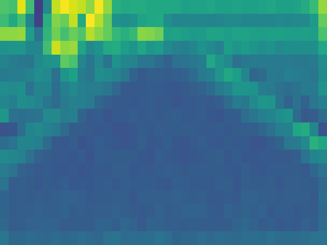
(d) 200

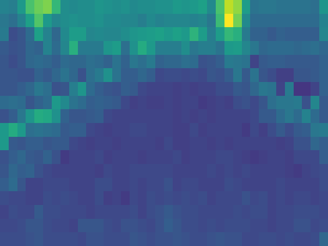
(e) 250

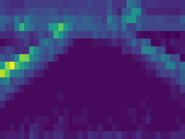
(f) 300

Figure 2: Forward heatmap plots at every 50 training epochs of end-to-end imitation learning. Brighter color represents more activation of neurons. After 300 iterations of training, the lanes (track boundaries) are more highlighted than other features. These plots emperically show that Assumption 1 holds.

We then further interpret this intermediate stage, the forward heatmap, as cost function-related important features that relate the input (observation) and the output (final optimal decision) under the optimal control settings. The averaged heatmap extracted from a middle convolutional layer of the trained E2EIL network is used to generate a costmap for MPC.

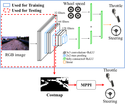
Figure 3: Blue box: The same structure used in [1] for IL training. For IRL testing, only the red-dashed part, from the image input to the second max pooling layer is used. This middle layer internally and implicitly learns the mapping from an input image to important features, which can be used as a costmap.

The training process is the same as the E2EIL controller [1]; AIRL only requires a dataset of images, wheel speed sensor readings, and the expert’s optimal solution to train a costmap model (see Figure 3).

Unlike [3, 4, 2], our method does not require access to a predetermined costmap function in order to train. Also, due to the fact that E2EIL can be taught from human data only [8], our approach can learn a cost function even without teaching specific task-related objectives to a model.

We generate a costmap from the activated middle layer neurons, which links the input image and the cost function. On top of that, we add a binary ($0$ or $1$) filter which outputs 1 if the activation is greater than 0, i.e. if it has some relevance scores. This binary filter is not a necessary step for an optimal controller, but rather heuristic to improve and robustify the performance. Even without the binary filter, the optimal controller eventually finds the optimal control policy that drives the robot to the drivable region but the binary filtering makes the costmap easier to optimize. The filtered costmap is more distinguishable between drivable region (0, black) and cost regions (1, white) as shown in Figure 1.

To describe the detailed dimensions used in AIRL, the input image size is $160\times 128\times 3$ and the output costmap from the middle layer after the second max-pooling (See Figure 3) is $40\times 32$. We tested the heatmaps from 3 middle layers in the CNN part, each of them were after each max-pooling layer. The 3 heatmaps have different sizes; $(80\times 64)$, $(40\times 32)$, and $(20\times 16)$. The feature activation was more distinguishable in deeper layers (smaller heatmaps) as the information flows towards the output. But the resolution of the smallest heatmap was too low to be used as a costmap, so we decided to use the heatmap with size $(40\times 32)$. This 2D costmap comes from taking the average of the activated neurons with respect to all 128 kernels ($128\times 40\times 32\times 3\rightarrow 40\times 32\times 3$), and converting the 3D RGB channel into grayscale ($40\times 32\times 3\rightarrow 40\times 32$). This is then resized to $160\times 128$ for MPPI costmap.

V EXPERIMENTS

V-A Data collection

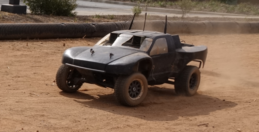
(a) The test vehicle

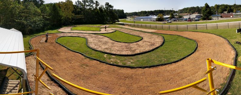
(b) Track A

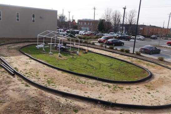
(c) Track B

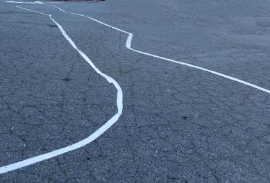
(d) Track C

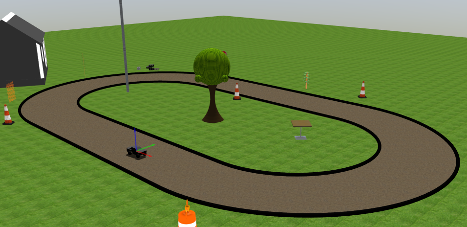
(e) Track D

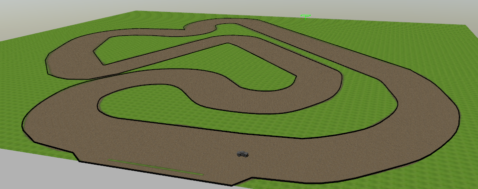
(f) Track E

Figure 4: a) The $1/5$ scaled ground vehicle used for experiments and b) the track used for training (Track A) and c-g) tracks used for testing (Track B, C, D, and E) Track D and E are from the ROS Gazebo simulator. Note that Track E is a simulated version of Track A, and Track D is a simulated version of Track B.

For a fair comparison, we trained all models with the same dataset used in [4]. The 90k data set consists of a vehicle running MPPI around a 170m-long track, the Track A. It includes various lighting conditions, and views on the track. Also shown in the supplementary video, the testing environment includes different shadow conditions and all the ruts, rocks, leaves, and grass on the dirt track provide various textures. With a learning rate of 0.001, Adam [25] was used as an optimizer for training. All the models converged with a training loss smaller than $5e^{-3}$ after $400$ epochs.

The rest of this section will explore how each method performed on each track. These methods were compared over various real and simulated datasets including the TORCS open source driving simulator [26] dataset and the KITTI dataset [27]. For the TORCS dataset, we used the baseline test set collected by [28]. All hardware experiments were conducted using our 1/5 scale autonomous vehicle test platform (Figure 4a) [29].

V-B Costmap Prediction

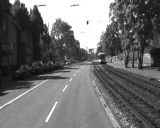
(a)

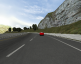
(b)

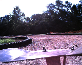
(c)

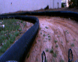
(d)

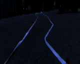
(e)

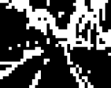
(f)

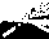
(g)

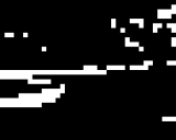
(h)

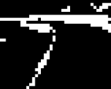
(i)

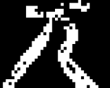
(j)

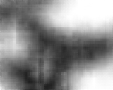
(k)

(l)

(m)

(n)

(o)

Figure 5: Top: From Left: KITTI, TORCS, Track A, Track B, and Track C. Middle: AIRL (ours) costmap generation. Bottom: Direct costmap prediction from ACP [2]. E2EIL does not provide a costmap output so it is not pictured here. Note that ACP works well on Track A data, which it was trained on.

We compare the methods mentioned in Section IV on the following scenarios:

1. Track A (real world complex track)

2. Track B (real world oval track)

3. Track C (real world pavement)

4. Track D (ROS gazebo, simulated Track B)

5. Track E (ROS gazebo, simulated Track A)

6. TORCS driving simulator [26]

7. KITTI dataset [27].

The pictures of each track can be found in Figure 4.

We first ran our proposed costmap model AIRL and the benchmark model ACP [2] on various datasets to show reasonable outputs in varied environments. The datasets used are KITTI, TORCs, Track A, Track B, and Track C as shown in Figure 5. AIRL produced costmaps that are interpretable by humans; Assumption 1 holds. The predicted costmap of the ACP is interpreted similarly to our method. The vehicle is located at the bottom middle of the costmap and black represents the low-cost region, white represents the high-cost. The difference is that ACP produces a top-down-view/bird-eye-view costmap, whereas our method, AIRL, produces a driver-view costmap. ACP produced clear cost maps models in Track A (which it was trained on) and Track C, though Track C’s costmap was incorrect. These results show an inability for ACP to generalize to varied different environments whereas our method produces similar looking costmaps throughout.

V-C Autonomous Driving

We then took all three methods and drove them on Tracks B, C, D, and E. Since it is too obvious and already reported in [2, 1], here we do not report how well each method does on training data (Track A). For Tracks B, D, and E, we ran each algorithm in both clockwise and counter-clockwise for 20 lap attempts and measured the average travel distance. We can see in Figure 6, that our approach was the only method that was able to finish the whole lap of driving Track B and D. Compared to other methods, our proposed method, AIRL, tended to hug track boundaries closely, presumably because of the sparsity of our costmaps.

The parameters used for AIRL’s MPPI in image space for all trials are as follows and they correspond to the original MPPI paper [18]: $\mathbf{K}=2,v_{x}^{d}=5.0m/s$ for off-road driving, $v_{x}^{d}=2.5m/s$ for on-road driving, $\Delta_{t}=0.02,\mathrm{T}=60,\Sigma_{steer}=0.3,\Sigma_{throttle}=0.35,C_{speed}=1.8$, and $C_{crash}=0.9$. $\mathrm{T}$ was set to correlate to approximately $6m$ long trajectories, as this covers almost all the drivable area in the camera view (see Figure 1c).

The benchmark method ACP failed to drive more than half of Track B because the predicted costmap was not stable as seen in Figure 5 Track B results. When looking at the costmaps generated from ACP in Figure 5, we can see that the model trained on Track A is not generating a clear costmap when tested on Track B.

We ensured that the poor performance of the benchmark model ACP was not due to improper tuning of MPPI by training another model of [2] on Track B data only. We then tuned MPPI with this model and drove it around Track B successfully for 10 laps straight before being manually stopped. After this verification of MPPI parameters, we applied the same parameters to ACP. Unfortunately, we did not see the same track coverage with properly tuned MPPI.

Overall, ACP performed best on Track E, which is a simulated version of the track it was trained upon, Track A. The other Tracks have a similar issue to Track B, i.e. unclear costmaps.

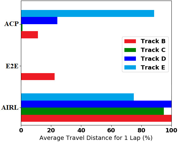
Figure 6: Generalization results of autonomous driving on tracks outside of the training dataset. AIRL (ours) outperforms the other two state-of-the-arts in most cases.

Surprisingly, the network trained through end-to-end imitation learning (E2EIL) was able to drive up to half of a lap on Track B, but in all of the sim datasets (Tracks D and E), it did not move. This is most likely due to images not matching the training distribution of images. The ability to drive on Track B is most likely due to the images being somewhat similar to Track A as can be seen in Figure 5.

We also verified the generalization of each method at a totally new on-road environment, Track C. We made a 30m-long zigzag lane on the tarmac to look like a real road situation. Since the training data was collected at Track A, an off-road dirt track, the tarmac surface is totally new; in addition, the boundaries of the course changed from black plastic tubes to taped white lanes. The width between the boundaries varied from 0.5 m to 1.5 m and was in general much tighter than the off-road tracks. Moreover, we ran our algorithm in the late afternoon, which has very different lighting conditions compared to the training data as seen in Figure 5. Even under this large change of environments, AIRL with MPPI was still able to accomplish a lane-keeping task most of the time, whereas the other two methods, E2EIL and ACP immediately failed the task.

VI DISCUSSION

We analyze that the false prediction of the benchmarks [1] and [2] comes from the covariate shift of the input image distribution. In the network trained through end-to-end imitation learning (E2EIL), although the middle layer outputs meaningful features/heatmap, a small change of each middle layer’s activation coming from a novel input results in a random or false NN output. For this reason, we cannot use the whole (same) NN parameters used in the E2EIL training phase. However, without throwing it away, we can still use the CNN portion of the original network for feature extraction. We saw in our experiments that the values of relevance scores of each pixel in the forward heatmap changes when it sees an out-of-sample input. This results in a failure of the output prediction of the whole DNN model. However, although the CNN parameters did not learn how much activation each neuron needs for data outside the training set, it surely learned the task-related feature extractions; the feature extractor part is still functional. Although the relevance ‘scores’ slightly changed, the activated ‘features’ are still unaffected. This is why AIRL shows great generalizability of producing a costmap. With a binary filter, it performs even better producing more distinguishable and robust costmaps.

VII CONCLUSION

We introduced an Approximate Inverse Reinforcement Learning framework using deep CNNs. By utilizing the powerful feature extracting nature of CNNs, our method automates the generalizable cost function learning through Imitation Learning by linking the extracted features to the cost function used in optimal control. Transferring pixel heatmaps of middle layers in a IL-trained network as a cost function holds the promises to automate the feature extraction and cost function design for other vision-based tasks as well. Beyond autonomous driving, any vision-based MDP problems, e.g. drones, legged robots, and manipulators with various tasks, are possible applications of the proposed approach.

Citations

Plain Text:

K. Lee, B. Vlahov, J. Gibson, J. M. Rehg, and E. A. Theodorou, “Approximate Inverse Reinforcement Learning from Vision-based Imitation Learning,” The 2021 International Conference on Robotics and Automation.

BibTeX:

@ARTICLE$\{$lee2021approximate,
author=$\{$Keuntaek $\{$Lee$\}$ and Bogdan $\{$Vlahov$\}$ and Jason $\{$Gibson$\}$ and James M. $\{$Rehg$\}$ and Evangelos A. $\{$Theodorou$\}$$\}$,
journal=$\{$The 2021 International Conference on Robotics and Automation$\}$,
title=$\{$$\{$Approximate Inverse Reinforcement Learning from Vision-based Imitation Learning$\}$$\}$,
year=$\{$2021$\}$
$\}$

References

- [1] Y. Pan, C.-A. Cheng, K. Saigol, K. Lee, X. Yan, E. A. Theodorou, and B. Boots, “Agile Autonomous Driving using End-to-End Deep Imitation Learning,” Robotics: Science and Systems, 2018.
- [2] P. Drews, “Visual Attention for High Speed Driving,” Ph.D. dissertation, Georgia Institute of Technology, 2019.
- [3] P. Drews, G. Williams, B. Goldfain, E. A. Theodorou, and J. M. Rehg, “Aggressive Deep Driving: Combining Convolutional Neural Networks and Model Predictive Control,” in 1st Annual Conference on Robot Learning, CoRL 2017, Mountain View, California, USA, November 13-15, 2017, Proceedings, 2017, pp. 133–142.
- [4] P. Drews, G. Williams, B. Goldfain, E. A. Theodorou, and J. M. Rehg, “Vision-Based High-Speed Driving With a Deep Dynamic Observer,” IEEE Robotics and Automation Letters, vol. 4, no. 2, pp. 1564–1571, 04 2019.
- [5] S. Levine, C. Finn, T. Darrell, and P. Abbeel, “End-to-End Training of Deep Visuomotor Policies,” Journal of Machine Learning Research, vol. 17, no. 39, pp. 1–40, 2016.
- [6] A. Giusti, J. Guzzi, D. Ciresan, F.-L. He, J. P. Rodriguez, F. Fontana, M. Faessler, C. Forster, J. Schmidhuber, G. Di Caro, D. Scaramuzza, and L. Gambardella, “A Machine Learning Approach to Visual Perception of Forest Trails for Mobile Robots,” IEEE Robotics and Automation Letters, 2016.
- [7] K. Lee, J. Gibson, and E. A. Theodorou, “Aggressive Perception-Aware Navigation using Deep Optical Flow Dynamics and PixelMPC,” IEEE Robotics and Automation Letters, 2020.
- [8] M. Bojarski, D. Del Testa, D. Dworakowski, B. Firner, B. Flepp, P. Goyal, L. D. Jackel, M. Monfort, U. Muller, J. Zhang, X. Zhang, J. Zhao, and K. Zieba, “End to End Learning for Self-Driving Cars,” arXiv, 04 2016.
- [9] H. Xu, Y. Gao, F. Yu, and T. Darrell, “End-to-end learning of driving models from large-scale video datasets,” in Proceedings of the IEEE conference on computer vision and pattern recognition, 2017, pp. 2174–2182.
- [10] M. Ollis, W. H. Huang, M. Happold, and B. A. Stancil, “Image-based path planning for outdoor mobile robots,” in 2008 IEEE International Conference on Robotics and Automation, 05 2008, pp. 2723–2728.
- [11] S. Arora and P. Doshi, “A survey of inverse reinforcement learning: Challenges, methods and progress,” arXiv preprint arXiv:1806.06877, 2018.
- [12] M. Babes, V. Marivate, M. Littman, and K. Subramanian., “Apprenticeship learning about multiple intentions.” in Proceedings of the 28th International Conference on Machine Learning, 2011.
- [13] M. Kuderer, S. Gulati, and W. Burgard, “Learning driving styles for autonomous vehicles from demonstration,” in 2015 IEEE International Conference on Robotics and Automation (ICRA), 05 2015, pp. 2641–2646.
- [14] S. Ross, G. J. Gordon, and J. A. Bagnell, “A Reduction of Imitation Learning and Structured Prediction to No-Regret Online Learning,” in Proceedings of the 14th International Conference on Artificial Intelligence and Statistics, ser. JMLR, vol. 15, Fort Lauderdale, FL, USA, 2011.
- [15] K. Lee, K. Saigol, and E. A. Theodorou, “Early failure detection of deep end-to-end control policy by reinforcement learning,” in 2019 International Conference on Robotics and Automation (ICRA), 05 2019, pp. 8543–8549.
- [16] K. Lee, Z. Wang, B. I. Vlahov, H. K. Brar, and E. A. Theodorou, “Ensemble bayesian decision making with redundant deep perceptual control policies,” 18th IEEE International Conference on Machine Learning and Applications (ICMLA), 2019.
- [17] K. Lee, G. N. An, V. Zakharov, and E. A. Theodorou, “Perceptual attention-based predictive control,” 3rd Conference on Robot Learning (CoRL), 2019.
- [18] G. Williams, N. Wagener, B. Goldfain, P. Drews, J. M. Rehg, B. Boots, and E. A. Theodorou, “Information theoretic MPC for model-based reinforcement learning,” in 2017 IEEE International Conference on Robotics and Automation (ICRA), 05 2017, pp. 1714–1721.
- [19] G. Williams, P. Drews, B. Goldfain, J. M. Rehg, and E. A. Theodorou, “Aggressive driving with model predictive path integral control,” 2016 IEEE International Conference on Robotics and Automation (ICRA), 2016.
- [20] E. Trucco and A. Verri, Introductory Techniques for 3-D Computer Vision. Upper Saddle River, NJ, USA: Prentice Hall PTR, 1998.
- [21] G. Montavon, W. Samek, and K.-R. Müller, “Methods for interpreting and understanding deep neural networks,” Digital Signal Processing, vol. 73, pp. 1 – 15, 2018.
- [22] W. Samek, G. Montavon, A. Vedaldi, L. K. Hansen, and K.-R. Müller, Explainable AI: Interpreting, Explaining and Visualizing Deep Learning. Springer, Cham, 2019, vol. 11700.
- [23] W. Samek, A. Binder, G. Montavon, S. Lapuschkin, and K. Müller, “Evaluating the Visualization of What a Deep Neural Network Has Learned,” IEEE Transactions on Neural Networks and Learning Systems, vol. 28, no. 11, pp. 2660–2673, 2017.
- [24] S. Bach, A. Binder, G. Montavon, F. Klauschen, K.-R. Müller, and W. Samek, “On Pixel-Wise Explanations for Non-Linear Classifier Decisions by Layer-Wise Relevance Propagation,” PLOS ONE, vol. 10, no. 7, 2015.
- [25] D. P. Kingma and J. Ba, “Adam: A Method for Stochastic Optimization,” Proceedings of the 3rd International Conference on Learning Representations (ICLR), vol. abs/1412.6980, 2014.
- [26] B. Wymann, C. Dimitrakakisy, A. Sumnery, and C. Guionneauz, “TORCS: The open racing car simulator,” 2015.
- [27] A. Geiger, P. Lenz, C. Stiller, and R. Urtasun, “Vision meets Robotics: The KITTI Dataset,” International Journal of Robotics Research (IJRR), 2013.
- [28] C. Chen, A. Seff, A. Kornhauser, and J. Xiao, “DeepDriving: Learning Affordance for Direct Perception in Autonomous Driving,” Proceedings of 15th IEEE International Conference on Computer Vision, 2015.
- [29] B. Goldfain, P. Drews, C. You, M. Barulic, O. Velev, P. Tsiotras, and J. M. Rehg, “AutoRally: An Open Platform for Aggressive Autonomous Driving,” IEEE Control Systems Magazine, vol. 39, no. 1, pp. 26–55, 02 2019.