Simulation of higher-order topological phases in 2D spin-phononic crystal networks

Abstract

We propose and analyse an efficient scheme for simulating higher-order topological phases of matter in two dimensional (2D) spin-phononic crystal networks. We show that, through a specially designed periodic driving, one can selectively control and enhance the bipartite silicon-vacancy (SiV) center arrays, so as to obtain the chiral symmetry-protected spin-spin couplings. More importantly, the Floquet engineering spin-spin interactions support rich quantum phases associated with topological invariants. In momentum space, we analyze and simulate the topological nontrivial properties of the one- and two-dimensional system, and show that higher-order topological phases can be achieved under the appropriate periodic driving parameters. As an application in quantum information processing, we study the robust quantum state transfer via topologically protected edge states. This work opens up new prospects for studying quantum acoustic, and offers an experimentally feasible platform for the study of higher-order topological phases of matter.

I introduction

Topological insulators (TIs) possess topologically protected surface or edge states, which can be utilized as robust transmission channels. In condensed matter physics, topological systems such as the quantum Hall effect and the quantum spin Hall effect have been extensively studied Hasan and Kane (2010); Thouless et al. (1982); Kane and Mele (2005). With the combination of topology and quantum theory, topological protection has developed some interesting applications in quantum information processing. In photonics, topological edge states can be used to realized one-way transport without breaking time reversal symmetry Lodahl et al. (2017); Barik et al. (2018); He et al. (2010); Peano et al. (2015); Haldane and Raghu (2008); Ozawa et al. (2019). In quantum computation, topology was introduced to solve the decoherence problem, in which the non-Abelian topological phases of matter are used to encode and manipulate quantum information Stern and Lindner (2013); Nayak et al. (2008); Xu et al. (2020).

The Su-Schrieffer-Heeger (SSH) model, originally derived from the dimerized chain, serves as the simplest example of one-dimensional (1D) topological insulator Su et al. (1979). So far, the SSH model have been realized in a number of quantum structures. For instance, a recent experiment demonstrated a tunable dimerized model and observed the topological magnon insulator states in a superconducting qubit chain Cai et al. (2019). As for ion-trap or optical lattice systems, an external periodic driving is generally needed to trigger the topological properties of the system, realizing the Floquet topological insulators in these systems Nevado et al. (2017); Creffield (2007); Pérez-González et al. (2019); Liu et al. (2019); Plekhanov et al. (2017). In addition, to investigate the topological characters of high-dimensional quantum devices, several theoretical works extended the SSH model to the two-dimensional (2D) case Yuce and Ramezani (2019); Zheng et al. (2019); Obana et al. (2019); Chen et al. (2019); Liu and Wakabayashi (2017); Xie et al. (2019). However, with the present experimental conditions, the observation of topological phenomena, in particular the higher-order topology, in the quantum domain is still challenging Yan (2019); Schindler et al. (2018); Zhang et al. (2019).

In recent years, quantum acoustics has aroused growing interests, which mainly studies the coherent interactions between quantized phonon modes and quantum emitters. Mechanical resonators or propagating phonons with low speed of sound in solids, offer unique advantages for transmitting quantum information between solid-state quantum systems. To date, experimental and theoretical progress has realized a variety of hybrid mechanical structures involving a large number of different quantum systems, such as solid-state defects Maity et al. (2020); Lemonde et al. (2018); Li et al. (2016, 2015); Li and Nori (2018); Bienfait et al. (2019); Kuzyk and Wang (2018); Li et al. (2017), superconducting circuits Etaki et al. (2008); Satzinger et al. (2018); Chu et al. (2018); LaHaye et al. (2009); Dong and Li (2019); Li et al. (2020a), ultracold atoms Camerer et al. (2011); Jöckel et al. (2015), and quantum dots Metcalfe et al. (2010); Yeo et al. (2014). Among these, due to the excellent coherence properties even at room temperature, defect spins in diamond and silicon carbide have become one of the most promising systems for quantum applications in solid states. In particular, the negatively charged silicon-vacancy (SiV) center in diamond serves as an emerging block for hybrid quantum systems because of high strain susceptibility and remarkable optical properties Meesala et al. (2018); Hepp et al. (2014); Sohn et al. (2018); Qiao et al. (2020).

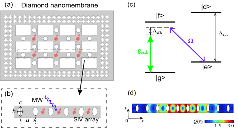
Figure 1: (Color online) (a) Schematics of the hybrid device studied in this work. Nanomechanical 2D phonon band-gap setups elaborately designed with high-Q cavities in a patterned diamond membrane. (b) Arrays of SiV color centers are implanted evenly in the phononic waveguide. The lattice constant of the phononic crystal is $a=100$ nm, the size of the ellipse hole are $(b,c)=(30,76)$ nm, and the thickness is $t=20$ nm. SiV spins are driven by microwave driving fields. (c) Ground-state energy levels of a single SiV center. Lower and upper states split via an external magnetic field. $g_{n,k}$ describes the coupling strength between the spin and the phonon with the transition $(|g\rangle\leftrightarrow|f\rangle)$, and $\Delta_{BE}=\omega_{s}-\omega_{BE}$ is the detuning between the spin transition and phononic band edge frequency. (d) Displacement pattern of the phononic compression mode at the band edge frequency $\omega_{BE}$.

Previous works have shown that a highly tunable spin-phonon interaction can be achieved near a phononic band gap Li et al. (2019, 2020b); Lemonde et al. (2019). Phononic crystals, defined as elastic waves propagating in periodic structures, which provide a powerful candidate for manipulating the interplay of phonons and other quantum systems. Because of the unique band structure of the phononic crystal, a single phonon bound state emerges within the band gap Liu and Houck (2017); John and Wang (1990); Krinner et al. (2018), resulting in a stronger and controllable spin-phonon coupling. More importantly, owing to the advantage of the scalable nature of nanofabrication, the spin-phononic crystal setup is experimentally feasible when extending to the higher dimensional case Chan et al. (2012); Burek et al. (2016); Kuang et al. (2004); Zhang and Liu (2004); Pennec et al. (2010); Sukhovich et al. (2008); Ding et al. (2019); Serra-Garcia et al. (2018); He et al. (2016); Safavi-Naeini et al. (2010); Lemonde et al. (2019); Peng et al. (2019).

In this work, we propose an efficient protocol for studying the topological quantum properties in 2D SiV-phononic crystal networks. Driving the SiV color center arrays with the periodic microwave fields, we obtain the Floquet engineering spin-spin interactions with some unique properties. We find that, it is possible to selectively control the phonon band-gap mediated spin-spin couplings by modulating the parameters of the periodic driving. We show that, the chiral symmetry-protected spin-spin interactions are attained in the bipartite SiV center arrays, and more importantly, the Floquet engineering spin-spin interactions support rich quantum topological phases. To investigate the topological nontrivial features of the system, we convert the 1D and 2D Floquet engineering spin-spin Hamiltonian to the momentum space. Firstly, we study the topological invariant Winding and Chern numbers, respectively. Apart from the original definitions, here we offer a geometrically intuitive way to calculate the topological invariant. And then we obtain the 1D and 2D topological Zak phases, respectively. We show that, the higher-order topological phase can be achieved under the appropriate periodic driving parameters. In addition, we give the analytical and numerical solutions of the topological edge states. Finally, we study the topological protected quantum state transfer and discuss the effect of SiV spin dephasing. This work offers an experimentally feasible platform for studying topological nontrivial phenomena in higher-dimensional quantum systems.

II 2D spin-phononic crystal networks

The 2D spin-phononic crystal setup is depicted in Fig. $1(a)$, where identical nodes are arranged in a square lattice. The diamond waveguide is perforated with periodic elliptical air holes, which yields the tunable phononic band structures. SiV color centers are evenly located at the nodes of the phononic structure, which are coupled to the acoustic vibrations via lattice strain. The pattern structure of the edge of the diamond membrane is designed to ensure the high-Q phonon band-gap cavities Chan et al. (2012).

For the phononic crystal, we first consider a quasi-1D geometry model, which supports acoustic guide modes $\omega_{n,k}$, with $n$ the band index and $k$ the wave vector along the waveguide direction. The mechanical displacement mode profile $\vec{Q}(\vec{r},t)$ can be obtained by solving the elastic wave equation Kushwaha et al. (1994). Analogous to the electromagnetic field in quantum optics, the mechanical displacement field can be quantized, i.e., $H_{p}=\sum_{n,k}\hbar\omega_{n,k}a_{n,k}^{\dagger}a_{n,k}$, with $a_{n,k}$ and $a_{n,k}^{\dagger}$ the annihilation and creation operators for the phonon modes.

SiV color centers are interstitial point defects wherein a silicon atom is positioned between two adjacent vacancies in the diamond lattice. The negatively charged SiV center can be treated as an effective $S=1/2$ system. For the electronic ground state of the SiV center, the $\left|{}^{2}E_{g}\right\rangle$ states are the combination of a twofold orbital and a twofold spin degeneracy. Considering the spin-orbit interaction and Jahn-Teller effect, the orbital states are separated into a lower branch (LB) and upper branch (UB) with frequency $\Delta_{GS}=2\pi\times 46$ GHz. In the presence of an external magnetic field $\vec{B}$, the Zeeman effect will be further split the spin degenerate states. The SiV ground state Hamiltonian can be written as Hepp et al. (2014)

$$H_{SiV}=-\hbar\lambda_{SO}L_{z}S_{z}+H_{JT}+\hbar f\gamma_{L}B_{z}L_{z}+\hbar\gamma_{S}\vec{B}\cdot\vec{S},$$ (1)

where $\lambda_{SO}$ is the strength of spin-orbit interaction, $\gamma_{L}$ and $\gamma_{S}$ correspond to the orbital and spin gyromagnetic ratio. Diagonalizing Eq. $(1)$, we obtain four eigenstates $\{\left|g\right\rangle=\left|e_{-}\downarrow\right\rangle,\left|e\right\rangle=\left|e_{+}\uparrow\right\rangle\},\{\left|f\right\rangle=\left|e_{+}\downarrow\right\rangle$ and $\left|d\right\rangle=\left|e_{-}\uparrow\right\rangle\}$, where $\left|e_{\pm}\right\rangle=(\left|e_{x}\right\rangle\pm i\left|e_{y}\right\rangle)/2$ are eigenstates of the orbital angular momentum operator. The corresponding energy level diagram is given in Fig. $1(c)$. As result, the spin-flip transitions are allowed between the four sublevels with opposite electronic spin components Becker et al. (2018); Pingault et al. (2017). Specifically, the two lowest sublevels $(|g\rangle,|e\rangle)$ can be treated as a long-lived qubit and coherently controlled via an optical Raman process. Furthermore, in the high-strain limit, this transition can be directly driven with a microwave field Nguyen et al. (2019).

In the SiV-phonon system, the mechanical lattice vibration modifies the electronic environment of the SiV center, resulting in the coupling of its orbital states $\left|e_{-}\right\rangle$ and $\left|e_{+}\right\rangle$. As for the setup shown in Fig. $1(b)$, when the transition frequency of the spin state is tuned close to the phononic band edge, we can obtain the strong strain coupling between the SiV center and phononic crystal mode Lemonde et al. (2018). By utilizing a microwave assisted Raman process involving the upper state $\left|f\right\rangle$, the transition of SiV electronic ground states $\left|g\right\rangle$ and $\left|e\right\rangle$ can be effectively coupled to the phononic mode. In this case, the spin-phonon interaction can be mapped to the Jaynes-Cummings model, namely

$$H_{s-p} = \sum_{n,k}\hbar\omega_{n,k}a_{n,k}^{\dagger}a_{n,k}+\hbar\omega_{s}\sigma_{ee}$$ (2)

$$+ \sum_{n,k}\hbar g_{n,k}(a_{n,k}\sigma_{eg}e^{ikx_{0}}+H.c.),$$

where $\sigma_{ij}=\left|i\right\rangle\langle j|$, $\omega_{s}$ is the effective spin transition frequency, $g\sim 0.1g_{n,k}$, and $g_{n,k}$ is the coupling strength between the SiV center and the phononic modes. Here, we consider that the defect centers are coupled predominantly to a single band of the phononic crystal, so the index $n$ be omitted in the following discussion. In Fig. $1(d)$, we numerically simulate the corresponding displacement pattern of the phononic mode by using the finite-element method (FEM), which is performed with the COMSOL MULTIPHYSICS software.

In a previous work, we proposed the band-gap engineered spin-phonon interaction. When the spin transition frequency is exactly in a phonon band gap, there will be a phononic bound state. Then we can obtain a much stronger SiV-phononic coupling via tuning the effective acoustic mode volume Li et al. (2019). In this context, we now study the interaction between the phononic crystal modes and an array of SiV spins. Here we assume that the SiV centers are equally coupled to the phononic mode near the band gap. Thus the interaction Hamiltonian of the defect spins and the phonon modes is expressed as

$$H_{I}=\sum_{j,k}\hbar g(a_{k}\sigma_{eg}^{j}e^{i\delta_{k}t+ikx_{j}}+H.c.),$$ (3)

with $\delta_{k}=\omega_{s}-\omega_{k}$. Assuming the large detuning regime, $\delta_{k}\gg g$, we can obtain an effective spin-spin interaction via adiabatically eliminate the phonon modes James and Jerke (2007). With the band gap engineered spin-phononic interaction, we integrate over the phononic modes and obtain the effective Hamiltonian

$$H_{array}=\sum_{i,j}\hbar J_{i,j}\sigma_{eg}^{i}\sigma_{ge}^{j},$$ (4)

where

$$J_{i,j}=\frac{g_{c}^{2}}{2\Delta_{BE}}e^{-|x_{i}-x_{j}|/L_{c}}$$ (5)

denotes the phononic band-gap mediated spin-spin interaction strength, and $\Delta_{BE}=\omega_{s}-\omega_{BE}$ is the detuning between the spin transition and the phononic band edge frequency. $g_{c}=g\sqrt{2\pi a/L_{c}}$ corresponds to the spin-phononic coupling strength, with $a$ the lattice constant and $L_{c}$ the localized length of phononic wavefunction. Going back to the two-dimensional setup shown in Fig. $1(a)$, we consider a phononic network with square lattices on the $x$-$y$ plane, with $2N\times 2N$ SiV spins located separately at the nodes of the phononic structure. Hence, the phononic mediated spin-spin interactions can be obtained as

$$H_{array}^{(2D)} = H_{array}^{(x)}+H_{array}^{(y)},$$

$$H_{array}^{(x)} = \overset{2N}{\sum_{l=1}}\overset{2N}{\sum_{i,j=1}}\hbar(J_{i,j}\sigma_{eg}^{(i,l)}\sigma_{ge}^{(j,l)}+H.c.),$$

$$H_{array}^{(y)} = \overset{2N}{\sum_{j=1}}\overset{2N}{\sum_{k,l=1}}\hbar(J_{k,l}\sigma_{eg}^{(j,k)}\sigma_{ge}^{(j,l)}+H.c.),$$ (6)

where $H_{array}^{(x)}$ and $H_{array}^{(y)}$ describe the effective spin-spin interactions in the $x$ and $y$ directions, respectively. $J_{i,j}$ and $J_{k,l}$ are the corresponding phonon mediated spin-spin hopping rates.

Note that different from the conventional dipole-dipole interaction mediated by a mechanical resonator or waveguide, this band-gap mediated spin-spin interaction is decay exponentially with the distance between spins, with a decay length $L_{c}$. This form of interparticle coupling ($J_{i,j}\sim e^{-|x_{i}-x_{j}|/\lambda}$) is commonly encountered in several other quantum systems, such as quantum dot and trapped-ion setups Nevado et al. (2017); Pérez-González et al. (2019). In the spin-phononic crystal system, owing to the unique band gap structures of the phononic crystal, we can get strong and tunable spin-spin interactions by controlling the mediated phononic modes.

III 1D topological properties

III.1 The periodic driving

The periodic driving is known to render effective Hamiltonian in which specific terms can be adiabatically eliminated. In particular, the periodic driving can be used to trigger nonequilibrium topological behavior in a trivial setup, which offers an efficient tool to simulate topological phases in quantum systems Goldman and Dalibard (2014); Gómez-León and Platero (2013). We consider a periodic driving quantum system with $H(t)=H(t+T)$, characterized by time period $T=2\pi/\omega$. In this case we can introduce Floquet theorem to investigate long-time dynamics of the system, as developed in Ref. Eckardt and Anisimovas (2015). With the Floquet-Bloch ansatz, the time-dependent Schrodinger equation be given by

$$i\hbar d_{t}\left|\psi_{\alpha}(t)\right\rangle=H(t)\left|\psi_{\alpha}(t)\right\rangle,$$ (7)

where

$$\left|\psi_{\alpha}(t)\right\rangle=\left|\phi_{\alpha}(t)\right\rangle e^{-i\epsilon_{\alpha}t/\hbar}=e^{-i\epsilon_{\alpha}t/\hbar}\sum_{m}e^{-im\omega t}\phi_{m}.$$ (8)

$\left|\psi_{\alpha}(t)\right\rangle$ is the so-called Floquet eigenstate, and $\epsilon_{\alpha}$ is the quasienergy with band index $\alpha$. $\phi_{\alpha}(t)=\phi_{\alpha}(t+T)$ denotes the time-periodic Floquet eigenmode, which can be constructed by a complete set of orthonormal basis state $\phi_{m}$. With respect to the basis $\left|\psi_{\alpha}(t)\right\rangle$, the system can be effectively described by the Hamiltonian

$$H_{eff}^{mn}=\frac{1}{T}\int_{0}^{T}dte^{i(m-n)\omega t}H(t)\text{.}$$ (9)

The effective Hamiltonian is the time-average of the Hamiltonian $H(t)$ in a driving period, which is the core of Floquet theorem. Note that the Floquet state in time-periodically driven systems is analogous to the Bloch state in spatially periodic systems.

In a recent work Li et al. (2020b), we proposed a periodic driving protocol to simulate topological phases with a color center-phononic crystal system. By applying a standing wave field between the two lowest sublevels ($|g\rangle,|e\rangle$) of the SiV center, we get the Floquet engineering of the spin-spin interactions, resulting in the well-known SSH-type Hamiltonian. Here we consider a fundamentally different driving protocol, which allows us to selectively control the spin-spin interactions. What is more important, the resulting spin-spin interactions possess chiral symmetry and support rich quantum phases associated with topological invariants. The time-periodic driving has form Pérez-González et al. (2019)

$$H_{driv}(t)=\sum_{j}\hbar V_{j}f(t)\sigma_{j}^{z},$$ (10)

where $\sigma_{j}^{z}=|e\rangle_{j}\langle e|-|g\rangle_{j}\langle g|$ is the Pauli operator component. $f(t)$ denotes the standard square-wave function

$$f(t) = -1\text{ \ \ \ for }t\in[0,\frac{T}{2}],$$

$$f(t) = 1\text{ \ \ \ \ for }t\in[\frac{T}{2},T].$$ (11)

$V_{j}$ denotes the on-site potential

$$V_{j}=\left\{\begin{array}[]{l}b_{0}+\frac{(a_{0}+b_{0})}{2}(j-1)\ \ \ \ j=1,3,5,7,...\\ \frac{(a_{0}+b_{0})}{2}j\ \ \ \ \ \ \ \ \ \ \ \ \ \ j=2,4,6,8,...\end{array}\right..$$ (12)

This stair-like form offers alternating potential difference between two adjacent spins, i.e., $V_{j}-V_{j-1}=a_{0}$ and $V_{j+1}-V_{j}=b_{0}$ are staggered along the spin array.

We first consider the interaction of the periodic driving and the 1D spin array, but the case of 2D will be studied in the next section. Now we transform the total Hamiltonian $H_{1D}=H_{array}+H_{driv}(t)$ into the interaction picture, with the unitary operator $U(t)=e^{-i\int_{0}^{t}d\tau H_{driv}(\tau)/\hbar}$. After the unitary transformation, we obtain

$$\sigma_{eg}^{j} \rightarrow e^{i\Delta_{j}(t)\sigma_{j}^{z}}\sigma_{eg}^{j}e^{-i\Delta_{j}(t)\sigma_{j}^{z}}=\sigma_{eg}^{j}e^{2i\Delta_{j}(t)},$$

$$\sigma_{ge}^{j} \rightarrow e^{i\Delta_{j}(t)\sigma_{j}^{z}}\sigma_{ge}^{j}e^{-i\Delta_{j}(t)\sigma_{j}^{z}}=\sigma_{ge}^{j}e^{-2i\Delta_{j}(t)},$$ (13)

with

$$\Delta_{j}(t) = V_{j}\int_{0}^{t}d\tau f(\tau)$$ (14)

$$= V_{j}\int_{0}^{t}d\tau[\underset{n\neq 0}{\sum}\frac{1}{n\pi i}(e^{-in\pi}-1)e^{in\omega\tau}],$$

where we expanded $f(t)$ into its Fourier series. In the interaction picture, the total Hamiltonian has the form as

$$H_{1D}=\underset{i,j}{\sum}\hbar J_{ij}(t)\sigma_{eg}^{i}\sigma_{ge}^{j},$$ (15)

where $J_{ij}(t)=J_{ij}e^{2i(\Delta_{i}(t)-\Delta_{j}(t))}$ is the hopping rate with a temporal periodicity, $J_{ij}(t)=J_{ij}(t+T)$. The Floquet components of the Hamiltonian ($14$) read

$$H_{1D}^{mn}=\underset{i,j}{\sum}\hbar J_{ij}^{mn}\sigma_{eg}^{i}\sigma_{ge}^{j},$$ (16)

$$J_{ij}^{mn}=\frac{1}{T}\int_{0}^{T}dtJ_{ij}(t)e^{i(m-n)\omega t}.$$ (17)

For the time-periodically driven system, $H_{1D}^{mn}$ can be expressed by the Floquet-Magnus expansion. In the high-frequency regime $\omega\gg J_{i,j}$, it is a good approximation to neglect the rapid oscillation of the external driving Rahav et al. (2003); Eckardt and Anisimovas (2015); Mikami et al. (2016). As a result, the spin-spin interaction can be given by the zeroth-order expansion term

$$\mathcal{J}_{ij}=J_{ij}\frac{i\omega}{2\pi(V_{i}-V_{j})}(e^{-i2\pi(V_{i}-V_{j})/\omega}-1).$$ (18)

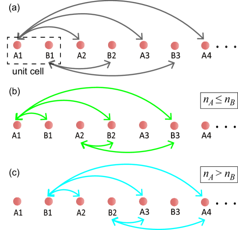
Figure 2: (Color online) Schematic diagram for effective spin-spin interactions. (a) Even-neighbor hopping. (b) and (c) illustrate two kinds of odd-neighbor hopping examples, respectively.

As for the SSH model, the interparticle interaction is characterized by staggering hopping amplitudes. Thus, the two nearest-neighbor spins can be grouped into a unit cell and classified as odd and even spins, as we proposed in Ref. Li et al. (2020b). Likewise, here we consider the phononic-mediated spin-spin interaction as a bipartite lattice of the form $ABABAB$, with

$$A_{n} = \sigma_{ge}^{j}\ \ \ j=1,3,5,7,...,$$

$$B_{n} = \sigma_{ge}^{j}\ \ \ j=2,4,6,8,....$$ (19)

Based on this definition, we rewrite the renormalized hopping amplitude $\mathcal{J}_{ij}$. For simplicity, here we introduce $n_{l}$ to label the spins at the $l$ site of the $n$th cell, $l=A$ or $B$. In general, there are two types of interparticle hopping. For the even-neighbor hopping, which describes the spin-spin interaction of the same sublattice, as shown in Fig. $2(a)$. The potential difference are $V_{i}-V_{j}=\pm m(a_{0}+b_{0})$, with $m=n_{l}^{\prime}-n_{l}$. In consequence, the even-neighbor spin-spin hopping rate can be written as

$$\mathcal{J}_{n_{l},n_{l}^{\prime}}=\frac{iJ_{n_{l},n_{l}^{\prime}}}{\mp 2\pi qm}(e^{\pm i2\pi qm}-1),$$ (20)

where $q=(a_{0}+b_{0})/\omega$, and “$\pm$” correspond to  the coupling to the right and left spins, respectively. From Eq. (20), the even-neighbor hopping is always zero if we assign $q=1,2,3,...$. Thus we conclude that the even-neighbor hopping can be suppressed by tuning the parameters $a_{0}$ and $b_{0}$. Note that the even-neighbor hopping is a detrimental source for the chiral symmetry Pérez-González et al. (2019).

For the odd-neighbor hopping, which describes the spin-spin interaction of the different sublattice. To better describe the physical picture of the spin-spin interaction, we further classify two kinds of odd-neighbor hopping. We first discuss the case with $n_{A}\leq n_{B}$, for which the schematic diagram is shown in Fig. $2(b)$. If we define $n_{B}=n_{A}+r$ $(r=0,1,2,...)$, the spin-spin interaction can be described by

$$\mathcal{J}_{n_{A},n_{B}} = -\frac{iJ_{n_{A},n_{B}}}{2\pi(qr+\frac{a_{0}}{\omega})}[e^{2i\pi(qr+\frac{a_{0}}{\omega})}-1],$$

$$\mathcal{J}_{n_{B},n_{A}} = \frac{iJ_{n_{A},n_{B}}}{2\pi(qr+\frac{a_{0}}{\omega})}[e^{-2i\pi(qr+\frac{a_{0}}{\omega})}-1],$$ (21)

where $\mathcal{J}_{n_{A},n_{B}}$ and $\mathcal{J}_{n_{B},n_{A}}$ describe the forward $(A\rightarrow B)$ and backward $(B\rightarrow A)$ hoppings, respectively. For the case with $n_{A}>n_{B}$, the schematic diagram is shown in Fig. $2(c)$. If we define $n_{B}=n_{A}-r^{\prime}$ $(r^{\prime}=1,2,3,...)$, the spin-spin interaction can be described by

$$\mathcal{J}_{n_{A},n_{B}}^{\prime} = \frac{iJ_{n_{A},n_{B}}}{2\pi(qr^{\prime}-\frac{a_{0}}{\omega})}[e^{-2i\pi(qr^{\prime}-\frac{a_{0}}{\omega})}-1],$$

$$\mathcal{J}_{n_{B},n_{A}}^{\prime} = -\frac{iJ_{n_{A},n_{B}}}{2\pi(qr^{\prime}-\frac{a_{0}}{\omega})}[e^{2i\pi(qr^{\prime}-\frac{a_{0}}{\omega})}-1].$$ (22)

Likewise, $\mathcal{J}_{n_{A},n_{B}}^{\prime}$ and $\mathcal{J}_{n_{B},n_{A}}^{\prime}$ represent the backward $(A\rightarrow B)$ and forward $(B\rightarrow A)$ hopping, respectively. From Eqs. (20) and (21), we can conclude

$$\mathcal{J}_{n_{A},n_{B}}=(\mathcal{J}_{n_{B},n_{A}})^{\ast},\mathcal{J}_{n_{A},n_{B}}^{\prime}=(\mathcal{J}_{n_{B},n_{A}}^{\prime})^{\ast}.$$ (23)

Unlike the case of the SSH model, the backward and forward hoppings of the odd-neighbor spin-spin interaction are not equal.

According to this bipartite solution, the Hamiltonian $H_{1D}$ can be rewritten as

$$H_{1D} = \underset{n,r,r^{\prime}}{\sum}\hbar(\mathcal{J}_{n_{A},n_{B}}A_{n}B_{n+r}^{\dagger}+\mathcal{J}_{n_{B},n_{A}}A_{n}^{\dagger}B_{n+r}$$ (24)

$$+\mathcal{J}_{n_{A},n_{B}}^{\prime}A_{n}B_{n-r^{\prime}}^{\dagger}+\mathcal{J}_{n_{B},n_{A}}^{\prime}A_{n}^{\dagger}B_{n-r^{\prime}}).$$

Here we neglected the even-neighbor hopping terms. By applying a particular periodic driving field to the SiV centers, we obtain the Floquet engineering of the spin-spin interactions with unique properties. In this case, the even-neighbor hopping is suppressed by tuning the parameters of the driving field, while the odd-neighbor hopping can be enhanced as needed. This scheme enforces the chiral symmetry which provides topological protection for the spin-spin interaction. In Fig. $3$, we numerically calculate the quasienergy spectrum as a function of $a_{0}$. We can see that all the eigenmodes are grouped into chiral symmetric pairs with opposite energies. For simplicity, here we express the bare spin-spin interaction as

$$J_{i,j}=\frac{g_{c}^{2}}{2\Delta_{BE}}e^{-|x_{i}-x_{j}|/L_{c}}=J_{0}e^{-|x_{i}-x_{j}|/L_{c}}.$$ (25)

Given that the band-gap mediated spin-spin interaction decays exponentially with the spin spacing, here only the first- and third- neighbor interactions are included.

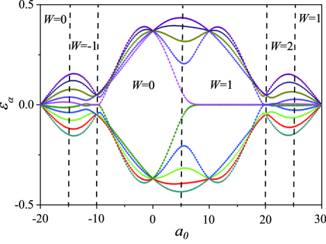
Figure 3: (Color online) (a) Quasienergy spectrum as a function of $a_{0}$, the corresponding winding number $\mathcal{W}$ is indicated. Here we assign $|x_{j}-x_{j+1}|=a$, $L_{c}=a$. Note that only the first and third odd-neighbor interactions are included. The other parameters are $N=5$, $\omega=10$, $q=1$ and $J_{0}=1$.

III.2 Topological phases

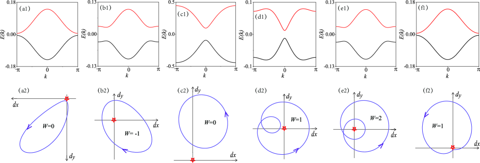
Figure 4: (Color online) (a1)-(f1) show the dispersion relations for various parameter settings of periodic driving: (a1) $a_{0}=-16$. (b1) $a_{0}=-11$. (c1) $a_{0}=4$. (d1) $a_{0}=19$. (e1) $a_{0}=21$. (f1) $a_{0}=26$. As the wave number $k$ runs through the Brillouin zone ($-\pi$, $\pi$), the energy spectrum splits into two branches and there exists a band gap between the lower and higher branches. (a2)-(f2) correspond to the winding configuration of $(d_{x},d_{y})$ around the origin (red star), and the relevant winding number $\mathcal{W}$ is explicitly shown. In (a2) and (c2), the loop wind avoids the origin, and then $\mathcal{W}=0$. In (b2), (d2) and (f2), the endpoint of $d(k)$ encircles the origin once, but these are topological inequivalent. For (d2) and (f2), the endpoint of $d(k)$ is a closed loop in the counter clockwise direction, and $\mathcal{W}=1$. While in (b2), the endpoint of $d(k)$ is along the clockwise direction, and $\mathcal{W}=-1$. In (e2), the endpoint of $d(k)$ encircles the origin two times, and $\mathcal{W}=2$. Other parameters are the same as those in Fig. $3$.

The periodic driving protocol offers an effective method to investigate the topological character of the spin-phononic crystal system. To explore topological features of the Floquet engineering spin-spin system, we convert $H_{1D}$ to the momentum space. Considering periodic boundary conditions, we can make the Fourier transformation

$$O_{n}=\frac{1}{\sqrt{N}}\sum_{k}e^{ink}O_{k},(O=A,B)$$ (26)

where $k=2\pi m/N(m=1,2,...,N)$ is the wavenumber in the first Brillouin zone, and $A_{k}$ and $B_{k}$ are the momentum space operators. Defining the unitary operator $\psi(k)=\left(\begin{array}[]{cc}A_{k}&B_{k}\end{array}\right)^{T}$, the Hamiltonian $H_{1D}$ be expressed as

$$H_{1D}=\sum_{k}\psi(k)^{\dagger}H(k)\psi(k).$$ (27)

Then we obtain $2\times 2$ matrix form of the Hamiltonian in the $k$-space

$$H(k)=\hbar\left(\begin{array}[]{cc}0&f(k)\\ f^{\ast}(k)&0\end{array}\right).$$ (28)

with

$$f(k)=\underset{r,r^{\prime}}{\sum}(\mathcal{J}_{n_{B},n_{A}}e^{ikr}+\mathcal{J}_{n_{B},n_{A}}^{{}^{\prime}}e^{-ikr^{\prime}}).$$ (29)

Here $f(k)$ describes the coupling between the $A$ and $B$ spins in momentum space.

The dispersion relation can be obtained by solving the eigenvalue equation

$$H(k)\psi(k)=E(k)\psi(k),$$ (30)

using the fact that $H^{2}(k)=E^{2}(k)I$, with $I$ being the identity operator in the Hilbert space. Then we obtain the energy band structure as

$$E(k)=\pm\hbar|f(k)|,$$ (31)

$$\psi(k)=\frac{1}{\sqrt{2}}\binom{1}{\pm e^{-i\vartheta(k)}}.$$ (32)

$\psi(k)$ corresponds to the eigenfunctions for the lower and upper band, and $\vartheta(k)$ is defined as the argument of $f(k)$. Figs. 4(a1)-(f1) show the energy spectra for different driving field parameters, which are split into two branches and there exists a band gap between the lower and upper branches. It should be noticed that the band gap will be vanished at the critical point of topological phases.

The band gap structures are generally associated with topological properties of bulk-boundary correspondence. For the 1D Floquet engineering spin-spin system, we introduce the topological Zak phase Shen et al. (2018)

$$\mathcal{\varphi}_{Zak} = -i\overset{occ.}{\underset{j=1}{\sum}}\int_{0}^{2\pi}dk\psi^{\dagger}(k)\partial_{k}\psi(k)$$ (33)

$$= N_{occ.}\frac{1}{2}\int_{0}^{2\pi}dk\frac{d}{dk}\vartheta(k)$$

$$= \mathcal{W}\pi$$

where $\mathcal{W}$ is the topological winding number, $N_{occ.}$ describes the number of occupied energy bands. Now we need to investigate the winding number of the system. Alternatively, $f(k)$ can be expressed in the form

$$f(k)=d(k)\cdot\sigma,$$ (34)

where $\sigma=(\sigma_{x},\sigma_{y},\sigma_{z})$ is the Pauli matrix, and $d(k)$ denotes a three-dimensional vector field

$$d_{x}(k) = \frac{1}{2}\underset{r,r^{\prime}}{\sum}(\mathcal{J}_{n_{B},n_{A}}e^{ikr}+\mathcal{J}_{n_{B},n_{A}}^{{}^{\prime}}e^{-ikr^{\prime}}+c.c.),$$

$$d_{y}(k) = \frac{i}{2}\underset{r,r^{\prime}}{\sum}(\mathcal{J}_{n_{B},n_{A}}e^{ikr}+\mathcal{J}_{n_{B},n_{A}}^{{}^{\prime}}e^{-ikr^{\prime}}-c.c.),$$

$$d_{z}(k) = 0.$$ (35)

For general $2$-band topological insulators, owing to the periodicity of the momentum-space Hamiltonian, the path of the endpoint of $d(k)$ is a closed loop in the auxiliary space $(d_{x},d_{y})$ Asbóth et al. (2016). The topology of this loop can be characterized by an integer, the winding number

$$\mathcal{W}=\frac{1}{2\pi}\int_{0}^{2\pi}\mathbf{n}\times\partial_{k}\mathbf{n}dk,$$ (36)

where $\mathbf{n}=(n_{x},n_{y})=(d_{x},d_{y})/\sqrt{d_{x}^{2}+d_{y}^{2}}$ is the normalized vector. Here the winding number $\mathcal{W}$ counts the number of times the loop winds around the origin of the $dx$-$dy$ plane. Figs. 4(a2)-(f2) present the path of the endpoint of $d(k)$ on the $dx$-$dy$ plane. For different values of $a_{0}$, the winding number of the system exhibits four possible values, $-1$, $0$, $1$, $2$. According to Eq. (33), we can derive the relevant topological Zak phases directly. Furthermore, one can implement the topological phase transition in this SiV-phononic system by modulating the periodic driving.

From the numerical simulation results, we show rich quantum phases related to topological invariants. As for the generalized SSH model, a prototypical example to investigate topological properties in a trivial system, the 1D Zak phase has only two possible values $0$ or $\pi$. This work offers an effective scheme for studying topological phases induced by periodic driving. The distinct feature is that it enables to simulate higher-order topological phases and related topological phase transitions in topological trivial systems.

III.3 Edge states

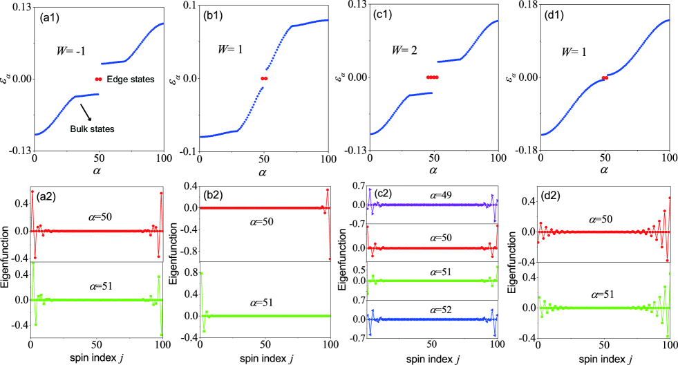
Figure 5: (Color online) (a1)-(d1) show the energy spectrum in the single-excited state subspace for various parameter settings of periodic driving: (a1) $a_{0}=-11$. (b1) $a_{0}=19$. (c1) $a_{0}=21$. (d1) $a_{0}=26$. For the cases with $\mathcal{W}=1$ and $\mathcal{W}=-1$, there are two zero-energy eigenvalues. For the case with $\mathcal{W}=2$, there are four zero-energy eigenvalues. The zero-energy eigenvalues (the red point) correspond to the topological edge states. The rest of eigenvalues (the blue point) correspond to the bulk states of the system. (a2)-(d2) show the related eigenfunction of the gapless modes. Here we consider $N=50$. Other parameters are the same as those in Fig. $3$.

The existence of edge states at the boundary is a distinguished feature for topological insulator states. In the following, we first simulate the edge states in a 1D spin-phononic system. The core step is to look for the zero-energy eigenstates. Here we introduce the single-excited state

$$\psi=\underset{n}{\sum}(a_{n}A^{\dagger}_{n}+b_{n}B^{\dagger}_{n})\left|0\right\rangle,$$ (37)

where $a_{n}$ and $b_{n}$ are the amplitudes of occupying probability in the $n$th cell. $\left|0\right\rangle=\left|ggg...\right\rangle$ is the vacuum state, which describes that all spins stay in the ground state $|g\rangle$. In the single-excited state subspace, we can get the the zero-energy eigenstates by sloving

$$H_{1D}\underset{n}{\sum}(a_{n}A^{\dagger}_{n}+b_{n}B^{\dagger}_{n})\left|0\right\rangle=0.$$ (38)

There will be $2N$ equations for the amplitudes $a_{n}$ and $b_{n}$. Considering the boundary conditions, $b_{0}=a_{N+1}=0$. We can analytically derive the left and right zero-energy edge states, respectively.

To verify the model, we numerically simulate the energy spectrum and zero-energy eigenstates of the system. Figs. 5(a1)-(d1) show the eigenvalues for various parameter settings of the periodic driving. As for the non-topological regime, $\mathcal{W}=0$, there will be an energy band gap but no gapless modes appear. For the cases with $\mathcal{W}=1$ and $\mathcal{W}=-1$, there are two zero-energy eigenvalues. For the case with $\mathcal{W}=2$, there are four zero-energy eigenvalues. Correspondingly, we plot the zero-energy edge states in Figs. 5(a2)-(d2). We see that the wavefunctions are located at the vicinity of the array boundaries, which are the so-called topological edge states. In addition, the edge states only distribute at certain (odd or even) sites, which is related to the chiral symmetry of the system.

IV 2D topological properties

IV.1 The periodic driving

Now we proceed to generalize the above 1D results to 2D spin-phononic crystal networks. Here we consider adding two mutually perpendicular microwave fields to the color center arrays Zou and Liu (2017). The first one is a time-dependent microwave driving of frequency $\omega_{x}$ in the $x$ direction. The other is a time-dependent driving of frequency $\omega_{y}$ in the $y$ direction. These two periodic driving fields have the form

$$H_{driv}^{(x)} = \overset{2N}{\sum_{l=1}}\overset{2N}{\sum_{j=1}}\hbar V_{j,l}f_{x}(t)\sigma_{j,l}^{z},$$

$$H_{driv}^{(y)} = \overset{2N}{\sum_{j=1}}\overset{2N}{\sum_{l=1}}\hbar V_{j,l}f_{y}(t)\sigma_{j,l}^{z}.$$ (39)

$V_{j,l}=(V_{j},V_{l})$ describes the on-site potential in the 2D phononic network, the two components of which are in the form of Eq. $(12)$. $f_{x}(t)$ and $f_{y}(t)$ denote the square-wave function in the $x$ and $y$ directions, respectively.

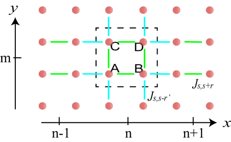
Figure 6: (Color online) Schematic diagram of the 2D Floquet engineering spin-spin interaction. There are four spins in a unit cell, which are labeled as {$A,B,C,D$}, respectively. Here we introduce $(n,m)$ to describe the position of each unit cell in the 2D spin-spin networks. For simplicity, only the nearest-neighbor interactions are illustrated.

Let us discuss the two directions separately. For the periodic driving spin arrays along the $x$ direction, the total Hamiltonian can be written as

$$H_{2D}^{(x)}=H_{array}^{(x)}+H_{driv}^{(x)}.$$ (40)

In the interaction picture, we introduce the unitary operator $U_{x}(t)=e^{-i\int_{0}^{t}d\tau H_{driv}^{(x)}/\hbar}$. After the unitary transformation, we obtain

$$\sigma_{eg}^{(j,l)}\rightarrow\sigma_{eg}^{(j,l)}e^{2i\Delta_{j}(t)},\sigma_{ge}^{(j,l)}\rightarrow\sigma_{ge}^{(j,l)}e^{-2i\Delta_{j}(t)},$$ (41)

with

$$\Delta_{j}(t)=V_{j}\int_{0}^{t}d\tau f(\tau).$$ (42)

While for the spin arrays along the $y$ direction, the total Hamiltonian is given by

$$H_{2D}^{(y)}=H_{array}^{(y)}+H_{driv}^{(y)}.$$ (43)

Similary, we introduce the unitary operator $U_{y}(t)=e^{-i\int_{0}^{t}d\tau H_{driv}^{(y)}/\hbar}$. After the unitary transformation, we obtain

$$\sigma_{eg}^{(j,l)}\rightarrow\sigma_{eg}^{(j,l)}e^{2i\Delta_{l}(t)},\sigma_{ge}^{(j,l)}\rightarrow\sigma_{ge}^{(j,l)}e^{-2i\Delta_{l}(t)},$$ (44)

with

$$\Delta_{l}(t)=V_{l}\int_{0}^{t}d\tau f(\tau).$$ (45)

In the following, analogous to the 1D case, we consider the bipartite interaction in both $x$ and $y$ directions. Then we get a 2D system with $N\times N$ unit cells. As depicted in Fig. $6$, there are four spins in each unit cell, which are labeled as {$A,B,C,D$}, respectively. In the regime $\omega\gg J_{i,j},J_{k,l}$, we derive the Floquet engineering spin-spin interactions along the $x$ and $y$ directions

$$H_{2D}^{(x)} = \underset{m}{\sum}\underset{n,r,r^{\prime}}{\sum}\hbar[\mathcal{J}_{n,n+r}(A_{n,m}B_{n+r,m}^{\dagger}+C_{n,m}D_{n+r,m}^{\dagger})$$

$$+\mathcal{J}_{n,n-r^{\prime}}^{\prime}(A_{n,m}B_{n-r^{\prime},m}^{\dagger}+C_{n,m}D_{n-r^{\prime},m}^{\dagger})+H.c.],$$

$$H_{2D}^{(y)} = \underset{n}{\sum}\underset{m,r,r^{\prime}}{\sum}\hbar[\mathcal{J}_{m,m+r}(A_{n,m}C_{n,m+r}^{\dagger}+B_{n,m}D_{n,m+r}^{\dagger})$$ (46)

$$+\mathcal{J}_{m,m-r^{\prime}}^{\prime}(A_{n,m}C_{n,m-r^{\prime}}^{\dagger}+B_{n,m}D_{n,m-r^{\prime}}^{\dagger})+H.c.].$$

For simplicity, we introduce $(n,m)$ to describe the position of each unit cell in the 2D spin-spin networks, with $n,m=1,2,\ldots,N$.

To simplify the model, here we suppose that the spin spacing $d_{x}=d_{y}$ and the periodic driving frequencies $\omega_{x}=\omega_{y}$. In this case, we can derive

$$\mathcal{J}_{n,n+r} = \mathcal{J}_{m,m+r},$$

$$\mathcal{J}_{n,n-r^{\prime}}^{\prime} = \mathcal{J}_{m,m-r^{\prime}}^{\prime}.$$ (47)

Thus we can define $s=n$ or $m$, and the two-dimensional Hamiltonian can be further integrated as

$$H_{2D} = \underset{r,r^{\prime}}{\sum}\underset{n,m}{\sum}\hbar[\mathcal{J}_{s,s+r}(A_{n,m}B_{n+r,m}^{\dagger}+C_{n,m}D_{n+r,m}^{\dagger}$$ (48)

$$+A_{n,m}C_{n,m+r}^{\dagger}+B_{n,m}D_{n,m+r}^{\dagger})$$

$$+\mathcal{J}_{s,s-r^{\prime}}^{\prime}(A_{n,m}B_{n-r^{\prime},m}^{\dagger}+C_{n,m}D_{n-r^{\prime},m}^{\dagger}$$

$$+A_{n,m}C_{n,m-r^{\prime}}^{\dagger}+B_{n,m}D_{n,m-r^{\prime}}^{\dagger})+H.c.].$$

IV.2 Topological phases

To investigate the topological features in the 2D Floquet engineering spin-spin system, we convert the Hamiltonian $H_{2D}$ to the momentum space. Here we consider periodic boundary conditions along both the $x$ and $y$ directions. Then we apply the Fourier transformation to the four spins in a unit cell

$$O_{n,m}=\frac{1}{\sqrt{N}}\sum_{\mathbf{k}}e^{i(k_{x}n+k_{y}m)}O_{\mathbf{k}},(O=A,B,C,D)$$ (49)

where $\mathbf{k}=(k_{x},k_{y})$ is the wavenumber in the first Brillouin zone. If we define the unitary operator $\psi(\mathbf{k})=\left(\begin{array}[]{cccc}A_{\mathbf{k}}&B_{\mathbf{k}}&C_{\mathbf{k}}&D_{\mathbf{k}}\end{array}\right)^{T}$, the two-dimensional Hamiltonian can be rewritten as

$$H_{2D}=\sum_{\mathbf{k}}\psi^{\dagger}(\mathbf{k})H(\mathbf{k})\psi(\mathbf{k}).$$ (50)

Along with that we get $4\times 4$ matrix form of the Hamiltonian in the $\mathbf{k}$-space

$$H(\mathbf{k})=\hbar\left(\begin{array}[]{cccc}0&f(k_{x})&f(k_{y})&0\\ f^{\ast}(k_{x})&0&0&f(k_{y})\\ f^{\ast}(k_{y})&0&0&f(k_{x})\\ 0&f^{\ast}(k_{y})&f^{\ast}(k_{x})&0\end{array}\right).$$ (51)

$f(k_{x})$ and $f(k_{y})$ have the same form as Eq. (29), which describe the spin-spin couplings in the $x$ and $y$ directions, respectively.

Let us study the 2D dispersion relation by solving the eigenvalue equation

$$H(\mathbf{k})\psi(\mathbf{k})=E(\mathbf{k})\psi(\mathbf{k}),$$ (52)

then obtain

$$E(\mathbf{k})=\epsilon_{x}\hbar\left|f(k_{x})\right|+\epsilon_{y}\hbar\left|f(k_{y})\right|,$$ (53)

$$\psi(\mathbf{k})=\frac{1}{2}\left(\begin{array}[]{c}1\\ \epsilon_{x}e^{-i\vartheta_{x}(k_{x})}\\ \epsilon_{y}e^{-i\vartheta_{y}(k_{y})}\\ \epsilon_{x}\epsilon_{y}e^{-i[\vartheta_{x}(k_{x})+\vartheta_{y}(k_{y})]}\end{array}\right),$$ (54)

where $\epsilon_{i}=\pm 1$, $\vartheta_{i}(k_{i})=\arg[f(k_{i})],$ $i=x,y$. In Figure. 7(a), we numerically calculate the 2D energy spectrum in the momentum space. There are four energy bands since there are four spins in a unit cell. The lowest and highest bands are isolated, while the two middle bands are jointed at the edges of the Brillouin zone ($0,0$), ($\pm\pi,\pm\pi$), ($\mp\pi,\pm\pi$). According to Eq. (53), there exist two equal energy band gaps. When assigning suitable values of $a_{0}$, these four bands will be jointed together, and the band gaps vanished. This is a signature of topological phase transition.

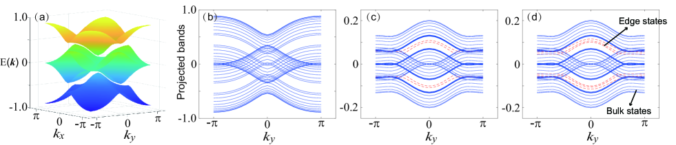
Figure 7: (Color online) (a) Band structure of the 2D Floquet engineering spin-spin interaction in the $\mathbf{k}$-space, $a_{0}=4$. The energy spectrum has four branches. The lowest and highest bands are isolated, while the two middle bands are touched at the edges of the Brillouin zone ($0,0$), ($\pm\pi,\pm\pi$), ($\mp\pi,\pm\pi$). (b)-(d) show the projected band structures for various parameter settings of periodic driving: (b) $a_{0}=4$. (c) $a_{0}=-11$. (d) $a_{0}=21$. The blue and red curves denote the bulk and edge modes, respectively. Here we consider $N_{x}=11$. Other parameters are the same as those in Fig. $3$.

For 2D systems, the topological invariants of energy bands are generally characterized by the Chern number. If we define the Bloch function $\psi_{m}(\mathbf{k})$ for the $m$th energy band, the non-Abelian Berry connection $A_{m}(\mathbf{k})=i\psi_{m}^{\dagger}(\mathbf{k})\partial_{\mathbf{k}}\psi_{m}(\mathbf{k})$. The topological Chern number can be calculated by the integral of $A_{m}(\mathbf{k})$ over the first Brillouin zone,

$$\mathcal{C}=\frac{1}{2\pi}\int_{BZ}d^{2}\mathbf{kTr}[A_{m}(\mathbf{k})].$$ (55)

The integral runs over all occupied bands. Alternatively, the Chern number can be defined by the vector field $d(\mathbf{k})$

$$\mathcal{C}=\frac{1}{4\pi}\int\int dk_{x}dk_{y}(\partial_{k_{x}}\mathbf{n}\times\partial_{k_{y}}\mathbf{n})\cdot\mathbf{n},$$ (56)

where $\mathbf{n}=d(\mathbf{k})/\left|d(\mathbf{k})\right|$. This implies that the topological invariant Chern number can be determined from the winding number in momentum space. Therefore, for this 2D periodically driving spin-spin interactions, the Chern number has four values, $-\frac{1}{2},0,\frac{1}{2},1$. It should be noted that the Chern number here is not quantized as an integer multiple, which is different from the traditional concept. For this reason, some works introduce a polarization vector to describe the topological invariant in the 2D system Yuce and Ramezani (2019); Chen et al. (2019); Liu and Wakabayashi (2017); Xie et al. (2019). As mentioned above, we consider the square lattice geometry, with the nearest-neighbor spin spacing $d_{x}=d_{y}$. Due to the $C_{4v}$ point group symmetry of the system, the corresponding 2D Zak phases are ($0,0$), ($\pm\pi,\pm\pi$), ($2\pi,2\pi$), while no such higher-order topological phases exist in the 2D SSH model.

IV.3 Edge states

After discussing the topological invariants, we are now in a position to study topological edge states in the 2D spin-phononic system. To show the behavior of edge states, here we consider a 2D strip structure with the periodic boundary condition in the $y$ direction and $N_{x}$ unit cells in the $x$ direction Wakabayashi et al. (2010); Wakabayashi and Dutta (2012). In this case, the Floquet engineering spin-spin interaction is translationally invariant only along the $y$ direction.

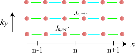
Figure 8: (Color online) Schematic diagram of the 2D spin-spin strip structure. After the Fourier transformation, there are a set of 1D spin-spin interaction arrays indexed by a continuous parameter $k_{y}$. For simplicity, only the nearest-neighbor interactions are illustrated.

As sketched in Fig. 8, after Fourier transformation in the $y$ direction, the two-dimensional strip can be reduced to a set of 1D spin-spin interactions indexed by a continuous parameter $k_{y}$. The two-dimensional Hamiltonian can be rewritten as

$$H_{2D}(k_{y}) = \underset{n,r,r^{\prime}}{\sum}\hbar[\mathcal{J}_{n,n+r}(A_{n}B_{n+r}^{\dagger}+C_{n}D_{n+r}^{\dagger}$$ (57)

$$+A_{n}C_{n}^{\dagger}e^{-ik_{y}r}+B_{n}D_{n}^{\dagger}e^{-ik_{y}r})$$

$$+\mathcal{J}_{n,n-r^{\prime}}^{\prime}(A_{n}B_{n-r^{\prime}}^{\dagger}+C_{n}D_{n-r^{\prime}}^{\dagger}$$

$$+A_{n}C_{n}^{\dagger}e^{ik_{y}r^{\prime}}+B_{n}D_{n}^{\dagger}e^{ik_{y}r^{\prime}})+H.c.],$$

with $n=1,2,\ldots,N_{x}$. In the single-excited state subspace

$$\psi(k_{y})=\underset{n}{\sum}(a_{n}A^{\dagger}_{n}+b_{n}B^{\dagger}_{n}+c_{n}C^{\dagger}_{n}+d_{n}D^{\dagger}_{n})\left|0\right\rangle,$$ (58)

where $a_{n},b_{n},c_{n},d_{n}$ denote the amplitudes of occupying probability in the $n$th cell, respectively. Substituting Eqs. (57)-(58) to the eigenvalue equation

$$H_{2D}(k_{y})\psi(k_{y})=E\psi(k_{y}),$$ (59)

we obtain the following set of equations of motion

$$Ea_{n} = f^{\ast}(k_{y})c_{n}+\mathcal{J}_{n,n+r}b_{n+r}+\mathcal{J}_{n,n-r^{\prime}}^{\prime}b_{n-r^{\prime}},$$

$$Eb_{n} = f^{\ast}(k_{y})d_{n}+\mathcal{J}_{n,n-r}a_{n-r}+\mathcal{J}_{n,n+r^{\prime}}^{\prime}a_{n+r^{\prime}},$$

$$Ec_{n} = f(k_{y})a_{n}+\mathcal{J}_{n,n+r}d_{n+r}+\mathcal{J}_{n,n-r^{\prime}}^{\prime}d_{n-r^{\prime}},$$

$$Ed_{n} = f(k_{y})b_{n}+\mathcal{J}_{n,n-r}c_{n-r}+\mathcal{J}_{n,n+r^{\prime}}^{\prime}c_{n+r^{\prime}}.$$ (60)

For the open boundaries $x=0,N_{x}+1$, the following amplitudes will be vanished,

$$b_{0} = d_{0}=0,$$

$$a_{N_{x}+1} = c_{N_{x}+1}=0.$$ (61)

In this way, we can analytically drive the edge modes.

In Figs. 7(b)-(d), we numerically calculate the resulting projected band structures with $N_{x}=11$. From the energy spectrum in the $k_{y}$ direction, we also verify the existence of edge states. The number of projected bands is determined by $N_{x}$. For the trivial case with $a_{0}=4$, there exist only the bulk modes (blue curves), no gapless modes emerge. While for the topological nontrivial case with $a_{0}=-11$ and $21$, we see that the edge modes (red dash lines) appear inside the energy band gaps. When $a_{0}=21$, the topological invariant winding number $\mathcal{W}=2$, and there are four zero-energy eigenstates, two of which are degenerated. In addition, we can also notice that the energy spectrum are symmetric with respect to the $E=0$, which is related to the chiral symmetry of the system.

V robust quantum state transfer

Topological nontrivial spin-spin interactions host zero-energy bound states at both ends. In the following, we show that the topological edge states can be employed as a quantum channel between distant qubits. Since quantum information can be transferred directly between the boundary spins, the intermediate spins are virtually excited during the process, which ensures the robust quantum state transfer Lemonde et al. (2019); Mei et al. (2018).

Taking into account the coupling of the system with the environment in the Markovian approximation, the evolution of the system follows the master equation

$$\dot{\rho}=-\frac{i}{\hbar}[H_{1D},\rho]+\overset{2N}{\sum_{j=1}}\gamma_{s}\mathcal{D}[\sigma_{j}^{z}]\rho,$$ (62)

with $\sigma_{j}^{z}=|e\rangle_{j}\langle e|-|g\rangle_{j}\langle g|$, $\gamma_{s}$ the spin dephasing rate of the single SiV centers, and $\mathcal{D}[O]\rho=O\rho O^{\dagger}-\frac{1}{2}\rho O^{\dagger}O-\frac{1}{2}O^{\dagger}O\rho$ for a given operator $O$.

To verify the theoretical results, we perform numerical calculations by using the QuTiP library for the 1D spin array with $N=3$. Here we take the excited left end spin as the initial condition. As illustrated in Fig. $9(a)$, we obtain the significant Rabi oscillation of the left end spin. This implies that there are indeed quantum state transfer between the two ends of the spin array. However, for the non-topological condition, no direct quantum state transfer can be seen, as shown in Fig. $9(c)$, since in the topological trivial regime, the eigenstates are the superposition of entire spin arrays. In addition, we simulate the excitation dynamics for different parameters of the periodic driving. Compared Fig. $9(a)$ with Fig. $9(b)$, we see that the localization of the edge states is more obvious when setting $a_{0}=12$. While for the case with $a_{0}=24$, it takes shorter time for accomplishing quantum state transfer. Finally, we also consider the effect of spin dephasing on quantum state transfer. As shown in Fig. $9(a)$, when setting the dephashing rate $\gamma_{s}=1\times 10^{-4}J_{0}$, which is closed to the practical experimental conditions, the fidelity can reach $0.9$. The numerical results can be optimized by adjusting the parameters of the periodic driving field.

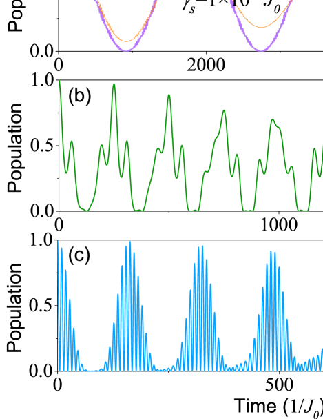
Figure 9: (Color online) Excitation dynamics of the left end spin for various parameter settings of periodic driving: (a) $a_{0}=12$. (b) $a_{0}=24$. (c) $a_{0}=-2$. In $(a)$, we also add the result in the case of $\gamma_{s}=1\times 10^{-4}J_{0}$. Here we consider $N=3$. Other parameters are the same as those in Fig. $3$.

VI Experimental feasibility

We consider a 2D spin-phononic crystal network, where SiV centers are individually embedded in the nodes of a phononic crystal with square geometry. Based on state-of-art nanofabrication techniques, several experiments have demonstrated the generation of color center arrays through ion implantation Toyli et al. (2010). The fabrication of nanoscale mechanical structures with diamond crystals has been realized experimentally, as proposed in Refs. Chan et al. (2012); Burek et al. (2016, 2017). Furthermore, owing to the advantage of the scalable nature of nanofabrication, the extension of phononic crystal structures to high dimensions is experimentally feasible, and extensive research has been conducted Pennec et al. (2010); Sukhovich et al. (2008); Ding et al. (2019); Serra-Garcia et al. (2018); He et al. (2016); Safavi-Naeini et al. (2010); Vasseur et al. (2001); Yang et al. (2004).

For the diamond phononic crystal illustrated in Fig. 1(a), the material properties are $E=1050$ GPa, $\nu=0.2$, and $\rho=3539$ kg/m³. The lattice constant and cross section of phononic crystal are $a=100$ nm and $A=100\times 20$ nm², and the sizes of the elliptical holes are $(b,c)=(30,76)$ nm. With these carefully designed parameters, we derive a phononic band edge frequency $\omega_{BE}/2\pi=44.933$ GHz. The ground state transition frequency of SiV center is about $46$ GHz, which is exactly located in a phononic band gap. The coupling between the SiV center and phononic crystal mode $k$ is given by $g_{k}=\frac{d}{v_{l}}\sqrt{\frac{\hbar\omega_{BE}}{4\pi\rho aA}}\xi(\vec{r})$ Sohn et al. (2018), where $d/2\pi\sim 1$ PHz is the strain sensitivity, $v_{l}=1.71\times 10^{4}$ m/s is the speed of sound in diamond, and $\xi(\vec{r})$ is the dimensionless strain distribution at the position of the SiV center $\vec{r}$. Here we assign $\xi(\vec{r})=1$ Safavi-Naeini et al. (2010). Then, we can obtain the effective SiV-phononic coupling rate as $g_{k}/2\pi\simeq 100$ MHz. In the large detuning regime, $g\sim 0.1g_{k}$, the band gap engineered spin-phononic coupling rate $g_{c}=g\sqrt{2\pi a/L_{c}}\simeq 2\pi\times 25$ MHz Li et al. (2019).

In addition, we should consider the decoherence of the SiV-phononic crystal setup. For the SiV color center in diamond, at mK temperatures, the spin dephasing time is about $\gamma_{s}/2\pi=100$ Hz Becker et al. (2018). As for phononic crystals, the mechanical quality factor is $Q\sim 10^{7}$, which can be achieved and further improved by using 2D phononic crystal shields Chan et al. (2012). In this case, we derive the mechanical dampling rate $\gamma_{m}/2\pi=4.5$ kHz. As calculated above, the band gap engineered spin-phononic coupling strength is $g_{c}/2\pi\simeq 25$ MHz, which considerably exceeds both $\gamma_{s}$ and $\gamma_{m}$, resulting in the strong strain interplay between the SiV centers and phonon crystal modes. For the nearest neighbour spins with $d_{0}=a$, the bare spin-spin interaction $J_{0}=\frac{g_{c}^{2}}{2\Delta_{BE}}\simeq 2\pi\times 4.1$ MHz. For the quantum state transfer in Fig. 9(a), the period is $\mathcal{T}=900/J_{0}\simeq 35$ $\mu$s, which is much shorter than the SiV spin coherence time ($T_{2}^{\ast}\sim 10$ ms) Sukachev et al. (2017). Therefore, with the practical experimental conditions, this proposal can be implemented to achieve high-fidelity quantum state transfer.

VII conclusion

To conclude, we explore the topological quantum properties in two-dimensional SiV-phononic crystal networks. Applying a special periodic drive to the SiV centers, the phononic band-gap mediated spin-spin interactions exhibit a topologically protected chiral symmetry. Then, we study the topological properties of the 1D and 2D Floquet engineering SiV center arrays, respectively. For the periodic driving with suitably chosen parameters, we analyse and simulate the corresponding topological invariants. We show that, under the appropriate driving fields, higher-order topological phases can be simulated in the spin-phononic crystal structures.

In contrast to the SSH model, the present Floquet engineering spin-spin interaction can be selectively controlled by modulating the periodic driving, which is essential for generating the necessary symmetries of the topological protection. More interestingly, we present rich topological Zak phases in this work. Owing to the highly controllable and tunable nature of the periodic driving, it is feasible to investigate the topological properties of the trimer case in SiV-phononic crystal systems. As an outlook, this proposal can be explored to study chiral quantum acoustics, topological quantum computing, and the implementation of hybrid quantum networks.

References

- Hasan and Kane (2010) M Zahid Hasan and Charles L Kane, “Colloquium: topological insulators,” Rev. Mod. Phys. 82, 3045 (2010).
- Thouless et al. (1982) David J Thouless, Mahito Kohmoto, M Peter Nightingale, and Md den Nijs, “Quantized hall conductance in a two-dimensional periodic potential,” Phys. Rev. Lett. 49, 405 (1982).
- Kane and Mele (2005) Charles L Kane and Eugene J Mele, “Quantum spin hall effect in graphene,” Phys. Rev. Lett. 95, 226801 (2005).
- Lodahl et al. (2017) Peter Lodahl, Sahand Mahmoodian, Søren Stobbe, Arno Rauschenbeutel, Philipp Schneeweiss, Jürgen Volz, Hannes Pichler, and Peter Zoller, “Chiral quantum optics,” Nature 541, 473 (2017).
- Barik et al. (2018) Sabyasachi Barik, Aziz Karasahin, Christopher Flower, Tao Cai, Hirokazu Miyake, Wade DeGottardi, Mohammad Hafezi, and Edo Waks, “A topological quantum optics interface,” Science 359, 666 (2018).
- He et al. (2010) Cheng He, Xiao-Lin Chen, Ming-Hui Lu, Xue-Feng Li, Wei-Wei Wan, Xiao-Shi Qian, Ruo-Cheng Yin, and Yan-Feng Chen, “Tunable one-way cross-waveguide splitter based on gyromagnetic photonic crystal,” Appl. Phys. Lett. 96, 111111 (2010).
- Peano et al. (2015) V Peano, C Brendel, M Schmidt, and F Marquardt, “Topological phases of sound and light,” Phys. Rev. X 5, 031011 (2015).
- Haldane and Raghu (2008) F. D. M Haldane and S Raghu, “Possible realization of directional optical waveguides in photonic crystals with broken time-reversal symmetry,” Phys. Rev. Lett. 100, 013904 (2008).
- Ozawa et al. (2019) Tomoki Ozawa, Hannah M Price, Alberto Amo, Nathan Goldman, Mohammad Hafezi, Ling Lu, Mikael C Rechtsman, David Schuster, Jonathan Simon, Oded Zilberberg, et al., “Topological photonics,” Rev. Mod. Phys. 91, 015006 (2019).
- Stern and Lindner (2013) Ady Stern and Netanel H Lindner, “Topological quantum computation from basic concepts to first experiments,” Science 339, 1179 (2013).
- Nayak et al. (2008) Chetan Nayak, Steven H Simon, Ady Stern, Michael Freedman, and Sankar Das Sarma, “Non-abelian anyons and topological quantum computation,” Rev. Mod. Phys. 80, 1083 (2008).
- Xu et al. (2020) Wen-Tao Xu, Qi Zhang, and Guang-Ming Zhang, “Tensor network approach to phase transitions of a non-abelian topological phase,” Phys. Rev. Lett. 124, 130603 (2020).
- Su et al. (1979) W. P. Su, J. R. Schrieffer, and A. J. Heeger, “Solitons in polyacetylene,” Phys. Rev. Lett. 42, 1698 (1979).
- Cai et al. (2019) Weizhou Cai, Jiaxiu Han, Feng Mei, Yuan Xu, Yuwei Ma, Xuegang Li, Haiyan Wang, YP Song, Zheng-Yuan Xue, Zhang-qi Yin, et al., “Observation of topological magnon insulator states in a superconducting circuit,” Phys. Rev. Lett. 123, 080501 (2019).
- Nevado et al. (2017) Pedro Nevado, Samuel Fernández-Lorenzo, and Diego Porras, “Topological edge states in periodically driven trapped-ion chains,” Phys. Rev. Lett. 119, 210401 (2017).
- Creffield (2007) C. E. Creffield, “Quantum control and entanglement using periodic driving fields,” Phys. Rev. Lett. 99, 110501 (2007).
- Pérez-González et al. (2019) Beatriz Pérez-González, Miguel Bello, Gloria Platero, and Álvaro Gómez-León, “Simulation of 1d topological phases in driven quantum dot arrays,” Phys. Rev. Lett. 123, 126401 (2019).
- Liu et al. (2019) Hui Liu, Tian-Shi Xiong, Wei Zhang, and Jun-Hong An, “Floquet engineering of exotic topological phases in systems of cold atoms,” Phys. Rev. A 100, 023622 (2019).
- Plekhanov et al. (2017) Kirill Plekhanov, Guillaume Roux, and Karyn Le Hur, “Floquet engineering of haldane chern insulators and chiral bosonic phase transitions,” Phys. Rev. B 95, 045102 (2017).
- Yuce and Ramezani (2019) C. Yuce and H. Ramezani, “Topological states in a non-hermitian two-dimensional su-schrieffer-heeger model,” Phys. Rev. A 100, 032102 (2019).
- Zheng et al. (2019) Li-Yang Zheng, Vassos Achilleos, Olivier Richoux, Georgios Theocharis, and Vincent Pagneux, “Observation of edge waves in a two-dimensional su-schrieffer-heeger acoustic network,” Phys. Rev. Appl. 12, 034014 (2019).
- Obana et al. (2019) Daichi Obana, Feng Liu, and Katsunori Wakabayashi, “Topological edge states in the su-schrieffer-heeger model,” Phys. Rev. B 100, 075437 (2019).
- Chen et al. (2019) Ze-Guo Chen, Changqing Xu, Rasha Al Jahdali, Jun Mei, and Ying Wu, “Corner states in a second-order acoustic topological insulator as bound states in the continuum,” Phys. Rev. B 100, 075120 (2019).
- Liu and Wakabayashi (2017) Feng Liu and Katsunori Wakabayashi, “Novel topological phase with a zero berry curvature,” Phys. Rev. Lett. 118, 076803 (2017).
- Xie et al. (2019) Bi-Ye Xie, Guang-Xu Su, Hong-Fei Wang, Hai Su, Xiao-Peng Shen, Peng Zhan, Ming-Hui Lu, Zhen-Lin Wang, and Yan-Feng Chen, “Visualization of higher-order topological insulating phases in two-dimensional dielectric photonic crystals,” Phys. Rev. Lett. 122, 233903 (2019).
- Yan (2019) Zhongbo Yan, “Higher-order topological odd-parity superconductors,” Phys. Rev. Lett. 123, 177001 (2019).
- Schindler et al. (2018) Frank Schindler, Ashley M Cook, Maia G Vergniory, Zhijun Wang, Stuart SP Parkin, B Andrei Bernevig, and Titus Neupert, “Higher-order topological insulators,” Sci. Adv. 4, eaat0346 (2018).
- Zhang et al. (2019) Xiujuan Zhang, Hai-Xiao Wang, Zhi-Kang Lin, Yuan Tian, Biye Xie, Ming-Hui Lu, Yan-Feng Chen, and Jian-Hua Jiang, “Second-order topology and multidimensional topological transitions in sonic crystals,” Nat. Phys. 15, 582 (2019).
- Maity et al. (2020) Smarak Maity, Linbo Shao, Stefan Bogdanović, Srujan Meesala, Young-Ik Sohn, Neil Sinclair, Benjamin Pingault, Michelle Chalupnik, Cleaven Chia, Lu Zheng, et al., “Coherent acoustic control of a single silicon vacancy spin in diamond,” Nat. Commun. 11, 193 (2020).
- Lemonde et al. (2018) M-A Lemonde, S Meesala, A Sipahigil, MJA Schuetz, MD Lukin, M Loncar, and P Rabl, “Phonon networks with silicon-vacancy centers in diamond waveguides,” Phys. Rev. Lett. 120, 213603 (2018).
- Li et al. (2016) Peng-Bo Li, Ze-Liang Xiang, Peter Rabl, and Franco Nori, “Hybrid quantum device with nitrogen-vacancy centers in diamond coupled to carbon nanotubes,” Phys. Rev. Lett. 117, 015502 (2016).
- Li et al. (2015) Peng-Bo Li, Yong-Chun Liu, S-Y Gao, Ze-Liang Xiang, Peter Rabl, Yun-Feng Xiao, and Fu-Li Li, “Hybrid quantum device based on n v centers in diamond nanomechanical resonators plus superconducting waveguide cavities,” Phys. Rev. Appl. 4, 044003 (2015).
- Li and Nori (2018) Peng-Bo Li and Franco Nori, “Hybrid quantum system with nitrogen-vacancy centers in diamond coupled to surface-phonon polaritons in piezomagnetic superlattices,” Phys. Rev. Appl. 10, 024011 (2018).
- Bienfait et al. (2019) Audrey Bienfait, Kevin J Satzinger, YP Zhong, H-S Chang, M-H Chou, Chris R Conner, É Dumur, Joel Grebel, Gregory A Peairs, Rhys G Povey, et al., “Phonon-mediated quantum state transfer and remote qubit entanglement,” Science 364, 368 (2019).
- Kuzyk and Wang (2018) Mark C Kuzyk and Hailin Wang, “Scaling phononic quantum networks of solid-state spins with closed mechanical subsystems,” Phys. Rev. X 8, 041027 (2018).
- Li et al. (2017) Xiao-Xiao Li, Peng-Bo Li, Sheng-Li Ma, and Fu-Li Li, “Preparing entangled states between two nv centers via the damping of nanomechanical resonators,” Sci. Rep. 7, 14116 (2017).
- Etaki et al. (2008) S Etaki, M Poot, I Mahboob, K Onomitsu, H Yamaguchi, and HSJ Van der Zant, “Motion detection of a micromechanical resonator embedded in a dc squid,” Nat. Phys. 4, 785 (2008).
- Satzinger et al. (2018) Kevin Joseph Satzinger, YP Zhong, H-S Chang, Gregory A Peairs, Audrey Bienfait, Ming-Han Chou, AY Cleland, Cristopher R Conner, Étienne Dumur, Joel Grebel, et al., “Quantum control of surface acoustic-wave phonons,” Nature 563, 661 (2018).
- Chu et al. (2018) Yiwen Chu, Prashanta Kharel, Taekwan Yoon, Luigi Frunzio, Peter T Rakich, and Robert J Schoelkopf, “Creation and control of multi-phonon fock states in a bulk acoustic-wave resonator,” Nature 563, 666 (2018).
- LaHaye et al. (2009) M. D LaHaye, J Suh, P. M Echternach, Keith C Schwab, and Michael L Roukes, “Nanomechanical measurements of a superconducting qubit,” Nature 459, 960 (2009).
- Dong and Li (2019) Xing-Liang Dong and Peng-Bo Li, “Multiphonon interactions between nitrogen-vacancy centers and nanomechanical resonators,” Phys. Rev. A 100, 043825 (2019).
- Li et al. (2020a) Peng-Bo Li, Yuan Zhou, Wei-Bo Gao, and Franco Nori, “Enhancing spin-phonon and spin-spin interactions using linear resources in a hybrid quantum system,” arXiv preprint arXiv:2003.07151 (2020a).
- Camerer et al. (2011) Stephan Camerer, Maria Korppi, Andreas Jöckel, David Hunger, Theodor W Hänsch, and Philipp Treutlein, “Realization of an optomechanical interface between ultracold atoms and a membrane,” Phys. Rev. Lett. 107, 223001 (2011).
- Jöckel et al. (2015) Andreas Jöckel, Aline Faber, Tobias Kampschulte, Maria Korppi, Matthew T Rakher, and Philipp Treutlein, “Sympathetic cooling of a membrane oscillator in a hybrid mechanical–atomic system,” Nat. Nano. 10, 55 (2015).
- Metcalfe et al. (2010) Michael Metcalfe, Stephen M Carr, Andreas Muller, Glenn S Solomon, and John Lawall, “Resolved sideband emission of InAs/GaAs quantum dots strained by surface acoustic waves,” Phys. Rev. Lett. 105, 037401 (2010).
- Yeo et al. (2014) Inah Yeo, Pierre-Louis De Assis, Arnaud Gloppe, Eva Dupont-Ferrier, Pierre Verlot, Nitin S Malik, Emmanuel Dupuy, Julien Claudon, Jean-Michel Gérard, Alexia Auffèves, et al., “Strain-mediated coupling in a quantum dot–mechanical oscillator hybrid system,” Nat. Nano. 9, 106 (2014).
- Meesala et al. (2018) Srujan Meesala, Young-Ik Sohn, Benjamin Pingault, Linbo Shao, Haig A Atikian, Jeffrey Holzgrafe, Mustafa Gündoğan, Camille Stavrakas, Alp Sipahigil, Cleaven Chia, et al., “Strain engineering of the silicon-vacancy center in diamond,” Phys. Rev. B 97, 205444 (2018).
- Hepp et al. (2014) Christian Hepp, Tina Müller, Victor Waselowski, Jonas N Becker, Benjamin Pingault, Hadwig Sternschulte, Doris Steinmüller-Nethl, Adam Gali, Jeronimo R Maze, Mete Atatüre, et al., “Electronic structure of the silicon vacancy color center in diamond,” Phys. Rev. Lett. 112, 036405 (2014).
- Sohn et al. (2018) Young-Ik Sohn, Srujan Meesala, Benjamin Pingault, Haig A Atikian, Jeffrey Holzgrafe, Mustafa Gündoğan, Camille Stavrakas, Megan J Stanley, Alp Sipahigil, Joonhee Choi, et al., “Controlling the coherence of a diamond spin qubit through its strain environment,” Nat. Commun. 9, 2012 (2018).
- Qiao et al. (2020) Yi-Fan Qiao, Hong-Zhen Li, Xing-Liang Dong, Jia-Qiang Chen, Yuan Zhou, and Peng-Bo Li, “Phononic-waveguide-assisted steady-state entanglement of silicon-vacancy centers,” Phys. Rev. A 101, 042313 (2020).
- Li et al. (2019) Peng-Bo Li, Xiao-Xiao Li, and Franco Nori, “Band-gap-engineered spin-phonon, and spin-spin interactions with defect centers in diamond coupled to phononic crystals,” arXiv:1901.04650 (2019).
- Li et al. (2020b) Xiao-Xiao Li, Bo Li, and Peng-Bo Li, “Simulation of topological phases with color center arrays in phononic crystals,” Phys. Rev. Research 2, 013121 (2020b).
- Lemonde et al. (2019) Marc-Antoine Lemonde, Vittorio Peano, Peter Rabl, and Dimitris G Angelakis, “Quantum state transfer via acoustic edge states in a 2d optomechanical array,” New J. Phys. 21, 113030 (2019).
- Liu and Houck (2017) Yanbing Liu and Andrew A Houck, “Quantum electrodynamics near a photonic bandgap,” Nat. Phys. 13, 48 (2017).
- John and Wang (1990) Sajeev John and Jian Wang, “Quantum electrodynamics near a photonic band gap: Photon bound states and dressed atoms,” Phys. Rev. Lett. 64, 2418 (1990).
- Krinner et al. (2018) Ludwig Krinner, Michael Stewart, Arturo Pazmino, Joonhyuk Kwon, and Dominik Schneble, “Spontaneous emission of matter waves from a tunable open quantum system,” Nature 559, 589 (2018).
- Chan et al. (2012) Jasper Chan, Amir H Safavi-Naeini, Jeff T Hill, Seán Meenehan, and Oskar Painter, “Optimized optomechanical crystal cavity with acoustic radiation shield,” Appl. Phys. Lett. 101, 081115 (2012).
- Burek et al. (2016) Michael J Burek, Justin D Cohen, Seán M Meenehan, Nayera El-Sawah, Cleaven Chia, Thibaud Ruelle, Srujan Meesala, Jake Rochman, Haig A Atikian, Matthew Markham, et al., “Diamond optomechanical crystals,” Optica 3, 1404 (2016).
- Kuang et al. (2004) Weimin Kuang, Zhilin Hou, and Youyan Liu, “The effects of shapes and symmetries of scatterers on the phononic band gap in 2d phononic crystals,” Phys. Lett. A 332, 481 (2004).
- Zhang and Liu (2004) Xiangdong Zhang and Zhengyou Liu, “Negative refraction of acoustic waves in two-dimensional phononic crystals,” Appl. Phys. Lett. 85, 341 (2004).
- Pennec et al. (2010) Yan Pennec, Jérôme O Vasseur, Bahram Djafari-Rouhani, Leonard Dobrzyński, and Pierre A Deymier, “Two-dimensional phononic crystals: Examples and applications,” Surf. Sci. Rep. 65, 229 (2010).
- Sukhovich et al. (2008) Alexey Sukhovich, Li Jing, and John H Page, “Negative refraction and focusing of ultrasound in two-dimensional phononic crystals,” Phys. Rev. B 77, 014301 (2008).
- Ding et al. (2019) Yujiang Ding, Yugui Peng, Yifan Zhu, Xudong Fan, Jing Yang, Bin Liang, Xuefeng Zhu, Xiangang Wan, and Jianchun Cheng, “Experimental demonstration of acoustic chern insulators,” Phys. Rev. Lett. 122, 014302 (2019).
- Serra-Garcia et al. (2018) Marc Serra-Garcia, Valerio Peri, Roman Süsstrunk, Osama R Bilal, Tom Larsen, Luis Guillermo Villanueva, and Sebastian D Huber, “Observation of a phononic quadrupole topological insulator,” Nature 555, 342 (2018).
- He et al. (2016) Cheng He, Xu Ni, Hao Ge, Xiao-Chen Sun, Yan-Bin Chen, Ming-Hui Lu, Xiao-Ping Liu, and Yan-Feng Chen, “Acoustic topological insulator and robust one-way sound transport,” Nat. Phys. 12, 1124 (2016).
- Safavi-Naeini et al. (2010) Amir H Safavi-Naeini, Thiago P Mayer Alegre, Martin Winger, and Oskar Painter, “Optomechanics in an ultrahigh-q two-dimensional photonic crystal cavity,” Appl. Phys. Lett. 97, 181106 (2010).
- Peng et al. (2019) Yu-Gui Peng, Ying Li, Ya-Xi Shen, Zhi-Guo Geng, Jie Zhu, Cheng-Wei Qiu, and Xue-Feng Zhu, “Chirality-assisted three-dimensional acoustic floquet lattices,” Phys. Rev. Research 1, 033149 (2019).
- Kushwaha et al. (1994) M. S. Kushwaha, P. Halevi, G. Martínez, L. Dobrzynski, and B. Djafari-Rouhani, “Theory of acoustic band structure of periodic elastic composites,” Phys. Rev. B 49, 2313 (1994).
- Becker et al. (2018) Jonas N. Becker, Benjamin Pingault, David Groß, Mustafa Gündoğan, Nadezhda Kukharchyk, Matthew Markham, Andrew Edmonds, Mete Atatüre, Pavel Bushev, and Christoph Becher, “All-optical control of the silicon-vacancy spin in diamond at millikelvin temperatures,” Phys. Rev. Lett. 120, 053603 (2018).
- Pingault et al. (2017) Benjamin Pingault, David-Dominik Jarausch, Christian Hepp, Lina Klintberg, Jonas N Becker, Matthew Markham, Christoph Becher, and Mete Atatüre, “Coherent control of the silicon-vacancy spin in diamond,” Nat. Commun. 8, 1 (2017).
- Nguyen et al. (2019) C. T Nguyen, D. D Sukachev, M. K Bhaskar, B Machielse, D. S Levonian, E. N Knall, P Stroganov, C Chia, M. J Burek, R Riedinger, H. Park, M. Lončar, and M. D. Lukin, “An integrated nanophotonic quantum register based on silicon-vacancy spins in diamond,” Phys. Rev. B 100, 165428 (2019).
- James and Jerke (2007) D. F James and Jonathan Jerke, “Effective hamiltonian theory and its applications in quantum information,” Can. J. Phys. 85, 625–632 (2007).
- Goldman and Dalibard (2014) Nathan Goldman and Jean Dalibard, “Periodically driven quantum systems: effective hamiltonians and engineered gauge fields,” Phys. Rev. X 4, 031027 (2014).
- Gómez-León and Platero (2013) Alvaro Gómez-León and Gloria Platero, “Floquet-bloch theory and topology in periodically driven lattices,” Phys. Rev. Lett. 110, 200403 (2013).
- Eckardt and Anisimovas (2015) André Eckardt and Egidijus Anisimovas, “High-frequency approximation for periodically driven quantum systems from a floquet-space perspective,” New J. Phys. 17, 093039 (2015).
- Rahav et al. (2003) Saar Rahav, Ido Gilary, and Shmuel Fishman, “Effective hamiltonians for periodically driven systems,” Phys. Rev. A 68, 013820 (2003).
- Mikami et al. (2016) Takahiro Mikami, Sota Kitamura, Kenji Yasuda, Naoto Tsuji, Takashi Oka, and Hideo Aoki, “Brillouin-wigner theory for high-frequency expansion in periodically driven systems: Application to floquet topological insulators,” Phys. Rev. B 93, 144307 (2016).
- Shen et al. (2018) Huitao Shen, Bo Zhen, and Liang Fu, “Topological band theory for non-hermitian hamiltonians,” Phys. Rev. Lett. 120, 146402 (2018).
- Asbóth et al. (2016) János K Asbóth, László Oroszlány, and András Pályi, “A short course on topological insulators,” Lecture notes in physics 919, 87 (2016).
- Zou and Liu (2017) Jin-Yu Zou and Bang-Gui Liu, “Quantum floquet anomalous hall states and quantized ratchet effect in one-dimensional dimer chain driven by two ac electric fields,” Phys. Rev. B 95, 205125 (2017).
- Wakabayashi et al. (2010) Katsunori Wakabayashi, Ken-ichi Sasaki, Takeshi Nakanishi, and Toshiaki Enoki, “Electronic states of graphene nanoribbons and analytical solutions,” Sci. Technol. Adv. Mater. 11, 054504 (2010).
- Wakabayashi and Dutta (2012) Katsunori Wakabayashi and Sudipta Dutta, “Nanoscale and edge effect on electronic properties of graphene,” Solid State Commun. 152, 1420 (2012).
- Mei et al. (2018) Feng Mei, Gang Chen, Lin Tian, Shi-Liang Zhu, and Suotang Jia, “Robust quantum state transfer via topological edge states in superconducting qubit chains,” Phys. Rev. A 98, 012331 (2018).
- Toyli et al. (2010) David M Toyli, Christoph D Weis, Gregory D Fuchs, Thomas Schenkel, and David D Awschalom, “Chip-scale nanofabrication of single spins and spin arrays in diamond,” Nano Lett. 10, 3168 (2010).
- Burek et al. (2017) Michael J Burek, Charles Meuwly, Ruffin E Evans, Mihir K Bhaskar, Alp Sipahigil, Srujan Meesala, Bartholomeus Machielse, Denis D Sukachev, Christian T Nguyen, Jose L Pacheco, et al., “Fiber-coupled diamond quantum nanophotonic interface,” Phys. Rev. Appl. 8, 024026 (2017).
- Vasseur et al. (2001) J. O Vasseur, Pierre A Deymier, B Chenni, B Djafari-Rouhani, L Dobrzynski, and D Prevost, “Experimental and theoretical evidence for the existence of absolute acoustic band gaps in two-dimensional solid phononic crystals,” Phys. Rev. Lett. 86, 3012 (2001).
- Yang et al. (2004) Suxia Yang, John H Page, Zhengyou Liu, Michael L Cowan, Che Ting Chan, and Ping Sheng, “Focusing of sound in a 3d phononic crystal,” Phys. Rev. Lett. 93, 024301 (2004).
- Sukachev et al. (2017) Denis D Sukachev, Alp Sipahigil, Christian T Nguyen, Mihir K Bhaskar, Ruffin E Evans, Fedor Jelezko, and Mikhail D Lukin, “Silicon-vacancy spin qubit in diamond: a quantum memory exceeding 10 ms with single-shot state readout,” Phys. Rev. Lett. 119, 223602 (2017).