Active Sentence Learning by Adversarial Uncertainty Sampling
in Discrete Space

Abstract

Active learning for sentence understanding aims at discovering informative unlabeled data for annotation and therefore reducing the demand for labeled data. We argue that the typical uncertainty sampling method for active learning is time-consuming and can hardly work in real-time, which may lead to ineffective sample selection. We propose adversarial uncertainty sampling in discrete space (AUSDS) to retrieve informative unlabeled samples more efficiently. AUSDS maps sentences into latent space generated by the popular pre-trained language models, and discover informative unlabeled text samples for annotation via adversarial attack. The proposed approach is extremely efficient compared with traditional uncertainty sampling with more than 10x speedup. Experimental results on five datasets show that AUSDS outperforms strong baselines on effectiveness.

1 Introduction

Deep neural models become popular in natural language processing Peters et al. (2018); Radford et al. (2018); Devlin et al. (2019). Neural models usually consume massive labeled data, which requires a huge quantity of human labors. But data are not born equal, where informative data with high uncertainty are decisive to decision boundary and are worth labeling. Thus selecting such worth-labeling data from unlabeled text corpus for annotation is an effective way to reduce the human labors and to obtain informative data.

Active learning approaches are a straightforward choice to reduce such human labors. Previous works, such as uncertainty sampling Lewis and Gale (1994), needs to traverse all unlabeled data to find informative unlabeled samples, which are always near the decision boundary with large entropy. However, the traverse process is very time-consuming, thus cannot be executed frequently Settles and Craven (2008). A common choice is to perform the sampling process after every specific period, and it samples and labels informative unlabeled data then trains the model until convergence Deng et al. (2018).

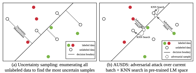
Figure 1: Comparison between uncertainty sampling and AUSDS for active learning.

We argue that infrequently performing uncertainty sampling may lead to the “ineffective sampling” problem. Because in the early phase of training, the decision boundary changes quickly, which makes previously collected samples less effective after several updates of the model. Ideally, uncertainty sampling should be performed frequently in the early phase of model training.

In this paper, we propose the adversarial uncertainty sampling in discrete space (AUSDS) to address the ineffective sampling problem for active sentence learning by introducing more frequent sampling with significantly lower costs. Specifically, we propose to leverage the adversarial attack Goodfellow et al. (2015); Kurakin et al. (2017) to the selecting of informative samples with high uncertainty, which significantly narrows down the search space. Fig. 1 shows the difference between uncertainty sampling and AUSDS. The typical uncertainty sampling (Fig. 1.a) traverses all the unlabeled samples to obtain samples of high uncertainty for each sampling run, which is costly with time complexity ($O({\rm Unlabeled~{}Data~{}Size})$. AUSDS (Fig. 1.b) first projects a labeled text to the decision boundary, denoted as an adversarial data point, and searches nearest neighbors of this point. The computational cost of AUSDS is significantly smaller than typical uncertainty sampling with the time complexity $O({\rm Batch~{}Size})$. But it is non-trivial for AUSDS to perform adversarial attacks, which requires adversarial gradients on sentences, since texts live in a discrete space. We propose to include a pre-trained neural encoder, such as BERT Devlin et al. (2019), to map unlabeled sentences into a continuous space, over which the adversarial attack is performed. Since not every adversarial data point in the encoding space can be mapped back to one of the unlabeled sentences, we propose to use the k-nearest neighbor (KNN) algorithm Altman (1992) to find the most similar unlabeled sentences (the adversarial samples) to the adversarial data points.Besides, empirically, we mix some random samples into the uncertainty samples to alleviate the sampling bias issue mentioned by Huang et al. (2010). Finally, the mixed samples are sent to an oracle annotator to obtain their label and are appended to the labeled data set.

We deploy AUSDS for active sentence learning and conduct experiments on five datasets across two NLP tasks, namely sequence classification and sequence labeling. Experimental results show that AUSDS outperforms random sampling and uncertainty sampling strategies.

Our contributions are summarized as follows:

• We propose AUSDS for active sentence learning, which first introduces the adversarial attack for sentence uncertainty sampling, alleviating the ineffective sampling problem.

• We propose to map sentences into the pre-trained LM encoding space, which makes adversarial uncertainty sampling available in the discrete sentence space.

• Experimental results demonstrate that our active sentence learning framework by AUSDS, which we call AUSDS learning framework, outperforms strong baselines in sampling effectiveness with acceptable running time.

2 Related Work

This work focuses on reducing the labeled data size with the help of pre-trained LM in solving sentence learning tasks. The proposed AUSDS approach is related to two different research topics, active learning and adversarial attack.

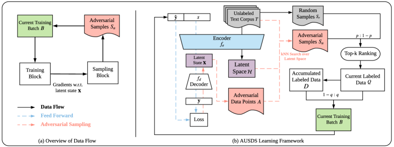
Figure 2: Overview of active sentence learning framework by AUSDS. Some notations are labeled along with corresponding components.

2.1 Active Learning

Active learning algorithms can be categorized into three scenarios, namely membership query synthesis, stream-based selective sampling, and pool-based active learning Settles (2009). Our work is more related to pool-based active learning, which assumes that there is a small set of labeled data and a large pool of unlabeled data available Lewis and Gale (1994). To reduce the demand for more annotations, the learner starts from the labeled data and selects one or more queries from the unlabeled data pool for the annotation, then learns from the new labeled data and repeats.

The pool-based active learning scenario has been studied in many real-world applications, such as text classification Lewis and Gale (1994); Hoi et al. (2006), information extraction Settles and Craven (2008) and image classification Joshi et al. (2009). Among the query strategies of existing active learning approaches, the uncertainty sampling strategy Joshi et al. (2009); Lewis and Gale (1994) is the most popular and widely used. The basic idea of uncertainty sampling is to enumerate the unlabeled samples and compute the uncertainty measurement like information entropy for each sample. The enumeration and uncertainty computation makes the sampling process costly and cannot be performed frequently, which induced the ineffective sampling problem.

There are some works that focus on accelerating the costly uncertainty sampling process. Jain et al. (2010) propose a hashing method to accelerate the sampling process in sub-linear time. Deng et al. (2018) propose to train an adversarial discriminator to select informative samples directly and avoid computing the rather costly sequence entropy. Nevertheless, the above works are still computationally expensive and cannot be performed frequently, which means the ineffective sampling problem still exists.

2.2 Adversarial Attack

Adversarial attacks are originally designed to approximate the smallest perturbation for a given latent state to cross the decision boundary Goodfellow et al. (2015); Kurakin et al. (2017). As machine learning models are often vulnerable to adversarial samples, adversarial attacks have been used to serve as an important surrogate to evaluate the robustness of deep learning models before they are deployed Biggio et al. (2013); Szegedy et al. (2014). Existing adversarial attack approaches can be categorized into three groups, which are one-step gradient-based approaches Goodfellow et al. (2015); Rozsa et al. (2016), iterative methods Kurakin et al. (2017) and optimization-based methods Szegedy et al. (2014).

Inspired by the similar goal of adversarial attacks and uncertainty sampling, in this paper, instead of considering adversarial attacks as a threat, we propose to combine these two approaches for achieving real-time uncertainty sampling. Some works share a similar but different idea with us. Li et al. (2018) introduce active learning strategies into black-box attacks to enhance query efficiency. Pal et al. (2020) also use active learning strategies to reduce the number of queries for model extraction attacks. Zhu and Bento (2017) propose to train Generative Adversarial Networks to generate samples by minimizing the distance to the decision boundary directly, which is in the query synthesis scenario different from us. Ducoffe and Precioso (2018) also introduce adversarial attacks into active learning by augmenting the training set with adversarial samples of unlabeled data, which is infeasible in discrete space. Note that none of the works above share the same scenario with our problem setting.

3 Active Sentence Learning with AUSDS

Algorithm 1 Active Sentence Learning with Adversarial Uncertainty Sampling in Discrete Space

Input: an unlabeled text corpus $T_{0}$, an oracle $O$, a labeled data $D_{0}=\{(s,O(s))|s\in S_{0},\text{ a small initial text corpus}\}$, pre-trained LM $f_{e}$, fine-tuning interval $j$, and fine-tuning step $k$.
Output: a well-trained model $f=(f_{e},f_{d})$

1:  Train $f_{d}$ on $D_{0}$ with frozen $f_{e}$;

2:  Construct a discrete bijective mapper $M$, where $M(s)=f_{e}(s)\in\mathcal{H}$ and $M^{-1}(f_{e}(s))=s\in T_{0}$;

3:  Sample a training batch $B_{0}$ from $D_{0}$;

4:  $i\leftarrow 0$

5:  while $|T_{i}|>0$ do

6:     Train decoder $f_{d}$ on $B_{i}$ with frozen encoder $f_{e}$;

7:     Generate adversarial data points $A\subset\mathcal{H}$ using the adversarial attack algorithm;

8:     Retrieve adversarial samples $S_{a}=\{s_{a}=M^{-1}(x)\in T_{i}|x\in\text{KNN}(A)\}$;

9:     Inject $S_{a}$ with random samples $S_{r}$, where $|S_{a}|:|S_{r}|=p:1-p$;

10:     Select top-k ranked samples $S_{add}$ from $S_{a}$ w.r.t. the information entropy;

11:     Label new data $Q\leftarrow\{(s,O(s))|s\in S_{add}\}$;

12:     Update labeled data $D_{i+1}\leftarrow D_{i}\cup Q$;

13:     Remove newly labeled data from unlabeled dataset $T_{i+1}\leftarrow T_{i}-S_{add}$;

14:     Sample a training batch $B_{i+1}$ from $Q$ and $D_{i+1}$ by the ratio of $q:1-q$;

15:     if $i$ mod $j=0$ then

16:        Fine-tune $f$ with $D_{i+1}$ for $k$ steps;

17:        Update the mapper $M$ with the fine-tuned encoder $f_{e}$ and text corpus $T_{i+1}$;

18:     end if

19:     $i\leftarrow i+1$

20:  end while

We propose AUSDS learning framework, an efficient and effective computational framework for active sentence learning. The overview of the learning framework is shown in Fig. 2. The learning framework consists of two blocks, a training block and a sampling block AUSDS. The training block learns knowledge from the labeled data, whereas the sampling block retrieves valuable unlabeled samples, whose latent states are close to the decision boundary over the latent space, from the unlabeled text corpus. Note that the definition of latent spaces can be different across encoders and tasks. The samples retrieved by the sampling block will be further sent to an oracle annotator to obtain their label, and the new samples with labels are also appended to the labeled data.

In this section, we first introduce AUSDS method by showing how AUSDS select samples that are critical to the decision boundary over the latent space. Then we present the computational procedure of the full-fledged framework in detail.

3.1 AUSDS

AUSDS first defines a latent space, over which sentences are distinguishable according to the model’s decision boundary. The latent space is usually determined by the encoder architecture and the downstream task. We detail the latent space definition of specific encoders and tasks in Sec. 4.1.

At first, we sample a batch of labeled texts and compute their representation as well as their gradients in the latent space. Using the latent states and their gradients, we perform adversarial attacks to generate adversarial data points $A$ near the decision boundary in the latent space. Adversarial attacks are performed using the following existing approaches:

• Fast Gradient Value (FGV) Rozsa et al. (2016): a one-step gradient-based approach with high efficiency. The adversarial data points are generated by:

  $$\mathbf{x}^{\prime}=\mathbf{x}+\lambda\cdot\nabla_{\mathbf{x}}F_{d}(\mathbf{x})$$ (1)

  where $\lambda$ is a hyper parameter, and $F_{d}$ is the cross entropy loss on $\mathbf{x}$.

• DeepFool Moosavi-Dezfooli et al. (2016): an iterative approach to find the minimal perturbation that is sufficient to change the estimated label.

• C&W Carlini and Wagner (2017): an optimization-based approach with the optimization problem defined as:

  $$\text{minimize }D(\mathbf{x},\mathbf{x}^{\prime})+c\cdot g(\mathbf{x}^{\prime})$$ (2)

  where $g(\cdot)$ is a manually designed function, satisfying $g(\mathbf{x})\leq 0$ if and only if $\mathbf{x}$’s label is a specific target label. $D$ is a distance measurement like Minkowski distance.

FGV is efficient in the calculation, whereas the other two methods typically find more precise adversarial data points but with larger computational costs. We use all of them in our experimental part to show the effectiveness of the AUSDS.

In our sentence learning scenario, the adversarial data points $A$ cannot be grounded on real natural language text samples. Thus we perform k-nearest neighbor (KNN) search Altman (1992) to find unlabeled text samples whose latent states are k-nearest to the adversarial data points $A$.

We implement the KNN search using Faiss Johnson et al. (2019), an efficient similarity search algorithm with GPUs. The computational cost of KNN search results from two processes, including constructing a sample mapper $M$ between text and latent space, and searching similar latent states of adversarial data points. The sampler mapper $M$ here is constructed as a hash map, which is of high computational efficiency, to memorize the mapping between an unlabeled text $s$ and its latent representation $\mathbf{x}$. The sample mapper is only reconstructed when the encoder is updated, and infrequent encoder updates contribute to efficiency. Besides, the searching process is also fast (100$\times$ faster than generating $A$) thanks to Faiss. Thus it is possible to performed AUSDS frequently at batch-level without harming computation.

After acquiring adversarial samples $S_{a}$ using KNN search, we mix $S_{a}$ with random samples $S_{r}$ drawn from unlabeled text corpus $T_{i}$ by the ratio of $p:1-p$, where $p$ is a hyper-parameter determined on the development set. The motivation of appending random samples is to balance exploration and exploitation, thus avoiding the model continuously retrieve samples in a small neighborhood.

We perform top-k ranking over the information entropy of the mixed samples to further retrieve samples with higher uncertainty. Since the size of the mixed samples is comparable to the batch size, the computation cost is acceptable. The remaining samples are further sent to an oracle annotator $O$ to obtain their labels.

3.2 Active Learning Framework

The overall procedure of the proposed framework equipped with AUSDS is outlined in Algorithm 1

Initialization

The initialization stage is shown in Algorithm 1 line 1-4. We first initialize our encoder $f_{e}$ with the pre-trained LM, which can be ${\rm BERT}_{\rm BASE}$ Devlin et al. (2019) or ${\rm ELMo}$ Peters et al. (2018). The decoder here is built upon the latent space and is randomly initialized. After building up the neural model architecture, we train only the decoder on existing labeled data $D_{0}$ to compute an initial decision boundary on the latent space. Meanwhile, we construct an initial discrete sample mapper $M$ used for the sampling block. Finally, we sample a training batch $B_{0}$ from labeled data corpus $D_{0}$, and set current training step $i$ to $0$.

Training

The training stage is shown in Algorithm 1 line 6. With the defined decoders $f_{d}$ and a training batch $B_{i}$, we train the decoder with a cross entropy loss (Fig. 2.b). Note that during the training process, we freeze the encoder as well as the latent space, where a frozen latent space contributes to computational efficiency without reconstructing the mapper $M$.

Sampling

The sampling stage is shown in Algorithm 1 line 7-14. As is shown in Sec. 3.1, given the gradients on the current batch $B_{i}$ w.r.t. latent states during training, the sampling process generates the adversarial samples $S_{a}$ and labels the samples with high uncertainty from a mixture of $S_{a}$ and randomly injected unlabeled data $S_{r}$. The labeled samples $Q$ are removed from the unlabeled text corpus and inserted into labeled data, resulting in $T_{i+1}$ and $D_{i+1}$ respectively. Then we create a new training batch consist of samples from $Q$ and $D_{i+1}$ with a ratio of $q:1-q$, which favors the newly selected data $Q$, because the newly selected ones are considered as more critical to the current decision boundary.

Fine-Tuning

The fine-tuning stage is shown in Algorithm 1 line 15-18. We fine-tune the encoder for $k$ steps after $j$ batches are trained. During the fine-tuning process, both of the encoder and the decoder are trained on the accumulated labeled data set $D_{i+1}$. The encoder is also fine-tuned for enhancing overall performance. Experiments show that the final performance is harmed a lot without updating the encoder. Then we update the mapper $M$ for the future KNN search, because the fine-tuning of the encoder corrupts the projection from texts to latent spaces, which requires renewal of the sampler mapper $M$. The algorithm terminates until the unlabeled text corpus $T_{i}$ is used up.

4 Experiments

We evaluate the AUSDS learning framework on sequence classification and sequence labeling tasks. For the oracle labeler $O$, we directly use the labels provided by the datasets. In all the experiments, we take average results of 5 runs with different random seeds to alleviate the influence of randomness.

Dataset	Task	Sample Size
SST-2 Socher et al. (2013)	sequence classification	11.8k sentences, 215k phrases
SST-5 Socher et al. (2013)	sequence classification	11.8k sentences, 215k phrases
MRPC Dolan et al. (2004)	sequence classification	5,801 sentence pairs
AG News Zhang et al. (2015)	sequence classification	12k sentences
CoNLL’03 Sang and De Meulder (2003)	sequence labeling	22k sentences, 300k tokens

Table 1: 5 datasets we used for sentence learning experiments, across sequence classification and sequence labeling tasks.

Dataset	RM	US	AUSDS(FGV)	AUSDS(DeepFool)	AUSDS(C&W)
SST-2	1061x	1x	38x	38x	28x
SST-5	1939x	1x	52x	52x	38x
MRPC	97x	1x	14x	14x	11x
AG News	1434x	1x	51x	47x	38x
CoNLL’03	45x	1x	10x	—	—

Table 2: The average speedup of each sampling step in comparison with US on 5 datasets with BERT as the encoder. The statistics are collected using Tesla-V100 GPU. US scans the unlabeled data once when 2% of data are labeled. The AUSDS using DeepFool and C&W on CoNLL’03 are omitted because these adversarial attack methods are not suitable for sequence labeling.

4.1 Set-up

Dataset.

We use five datasets, namely Stanford Sentiment Treebank (SST-2 / SST-5) Socher et al. (2013), Microsoft Research Paraphrase Corpus (MRPC) Dolan et al. (2004), AG’s News Corpus (AG News) Zhang et al. (2015) and CoNLL 2003 Named Entity Recognition dataset (CoNLL’03) Sang and De Meulder (2003) for experiments. The statistics can be found in Table 1. The train/development/test sets follow the original settings in those papers. We use accuracy for sequence classification and f1-score for sequence labeling as the evaluation metric.

Baseline Approaches.

We use two common baseline approaches in NLP active learning to compare with our framework, namely random sampling (RM) and entropy-based uncertainty sampling (US). For sequence classification tasks, we adopt the widely used Max Entropy (ME) Berger et al. (1996) as uncertainty measurement:

$$H^{ME}(\mathbf{x})=-\sum_{m=1}^{c}P(\mathbf{y}=m|\mathbf{x})\log P(\mathbf{y}=m|\mathbf{x})$$ (3)

where $c$ is the number of classes. For sequence labeling tasks, we use total token entropy (TTE) Settles and Craven (2008) as uncertainty measurement:

$$H^{TTE}(\mathbf{x})=-\sum_{i=1}^{N}\sum_{m=1}^{l}P(\mathbf{y}_{i}=m|\mathbf{x})\log P(\mathbf{y}_{i}=m|\mathbf{x})$$ (4)

where $N$ is the sequence length and $l$ is the number of labels.

Latent Space Definition

We use the adversarial attack in our AUSDS learning framework to find informative samples, which rely on a well-defined latent space. Two types of latent spaces are defined here based on the encoder architectures and tasks:

1. For pre-trained LMs like BERT Devlin et al. (2019), which has an extra token [CLS] for sequence classification, we directly use its latent state $\mathbf{x}$ as the representation of the whole sentence in the latent space $\mathcal{H}$.

2. For the other circumstances where no such special token can be used, a mean-pooling operation is applied to the encoder output, i.e. $\mathbf{x}=\frac{1}{n}\sum_{t=1}^{n}h_{t}$, where $h_{t}$ denotes the contextual word representation of the $t_{\text{th}}$ token produced by the encoder. The latent space $\mathcal{H}$ is spanned by all the latent states.

	Label Size	2%	4%	6%	8%	10%
SST-2	RM	87.78(.003)	89.85(.004)	89.85(.010)	89.69(.004)	90.26(.008)
	US	87.74(.004)	90.25(.006)	90.38(.008)	90.25(.006)	91.27(.007)
	AUSDS (FGV)	89.18(.002)	89.88(.008)	89.16(.014)	91.07(.005)	89.95(.003)
	AUSDS (DeepFool)	88.74(.004)	90.06(.003)	89.84(.007)	90.74(.006)	91.58(.002)
	AUSDS (C&W)	87.97(.003)	89.95(.005)	90.83(.007)	90.12(.003)	91.13(.001)
SST-5	RM	49.45(.010)	50.01(.007)	50.88(.006)	50.39(.014)	51.35(.005)
	US	49.10(.008)	49.54(.009)	50.63(.008)	50.90(.012)	51.43(.005)
	AUSDS (FGV)	49.57(.006)	50.36(.008)	50.09(.009)	50.19(.014)	50.62(.011)
	AUSDS (DeepFool)	50.20(.012)	51.87(.003)	51.74(.012)	50.97(.012)	51.23(.007)
	AUSDS (C&W)	48.28(.012)	48.78(.014)	51.58(.007)	51.40(.010)	47.42(.006)
MRPC	RM	67.33(.008)	68.31(.006)	68.56(.018)	70.06(.021)	71.15(.020)
	US	62.14(.090)	69.34(.005)	69.11(.010)	70.53(.017)	71.49(.016)
	AUSDS (FGV)	68.89(.014)	69.30(.023)	70.28(.015)	70.06(.012)	69.30(.019)
	AUSDS (DeepFool)	67.92(.009)	68.88(.017)	69.68(.017)	71.69(.014)	71.55(.012)
	AUSDS (C&W)	67.91(.014)	68.53(.017)	70.46(.012)	70.49(.012)	68.89(.016)
AG News	RM	89.89(.003)	90.89(.002)	91.37(.002)	91.79(.002)	92.21(.002)
	US	90.29(.006)	91.59(.007)	92.34(.003)	92.71(.001)	93.01(.001)
	AUSDS (FGV)	90.75(.002)	91.55(.002)	92.26(.003)	92.62(.001)	93.16(.001)
	AUSDS (DeepFool)	90.67(.004)	91.65(.004)	92.43(.004)	92.66(.004)	93.12(.002)
	AUSDS (C&W)	90.24(.002)	91.29(.002)	92.30(.004)	92.90(.002)	93.10(.003)
CoNLL’03	RM	80.42(.002)	83.38(.002)	85.39(.005)	86.78(.005)	87.42(.003)
	US	78.12(.002)	81.49(.019)	84.45(.004)	86.73(.008)	87.79(.004)
	AUSDS (FGV)	80.65(.006)	83.60(.003)	85.98(.010)	87.10(.004)	87.83(.003)
	AUSDS (DeepFool)	—	—	—	—	—
	AUSDS (C&W)	—	—	—	—	—

Table 3: The convergence results w.r.t. the label size in the training from scratch setting with BERT as the encoder. The label size denotes for the ratio of labeled data. The numbers are the averaged results of 5 runs on the test set. The best results with each label size are marked as bold. The sequence classification and sequence labeling tasks are evaluated with accuracy and f1 score, respectively. The AUSDS using DeepFool and C&W on CoNLL’03 are omitted because these adversarial attack methods are not suitable for sequence labeling.

Label Size	2%	4%	6%	8%	10%
RM	81.58(.004)	82.90(.006)	83.53(.008)	82.15(.016)	84.40(.006)
US	78.23(.007)	80.34(.003)	81.99(.006)	82.34(.008)	82.21(.004)
AUSDS (FGV)	81.22(.004)	83.25(.001)	84.18(.005)	84.49(.004)	84.62(.009)
AUSDS (DeepFool)	82.37(.003)	83.31(.004)	83.77(.002)	84.68(.001)	84.73(.005)
AUSDS (C&W)	81.27(.006)	84.02(.007)	82.76(.002)	84.40(.002)	83.58(.012)

Table 4: The convergence results w.r.t. the label size in the training from scratch setting with ELMo as encoder on SST-2. The label size denotes for the ratio of labeled data. The best results with each label size are marked as bold.

Implementation Details.

We implement our frameworks based on ${\rm BERT}_{\rm BASE}$ model and ${\rm ELMo}$. The configurations of the two models are the same as reported in Devlin et al. (2019) and Peters et al. (2018) respectively. The implementation of the KNN search is introduced in section 3.3. For the rest hyperparameters in our framework, 1) the batch size and the size of $Q$ is set as 32 (16 on MRPC dataset);  2) the fine-tuning interval $j$ and the fine-tuning step size $k$ are set as 50 steps;  3) the ratio $q$ is set as 0.3. All the tuning experiments are performed on the dev sets of five datasets. The accumulated labeled data set $D$ is initialized the same for different approaches, taking 0.1% of the whole unlabeled data (0.5% for MRPC because the dataset is relatively small).

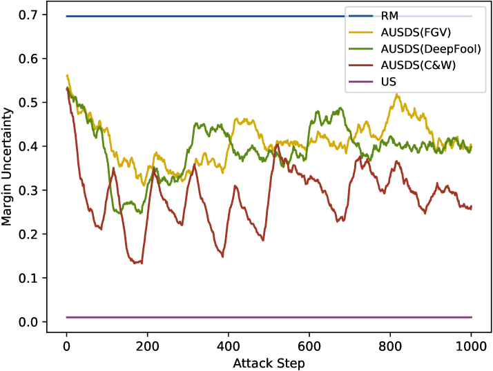
(a) Margin during Training

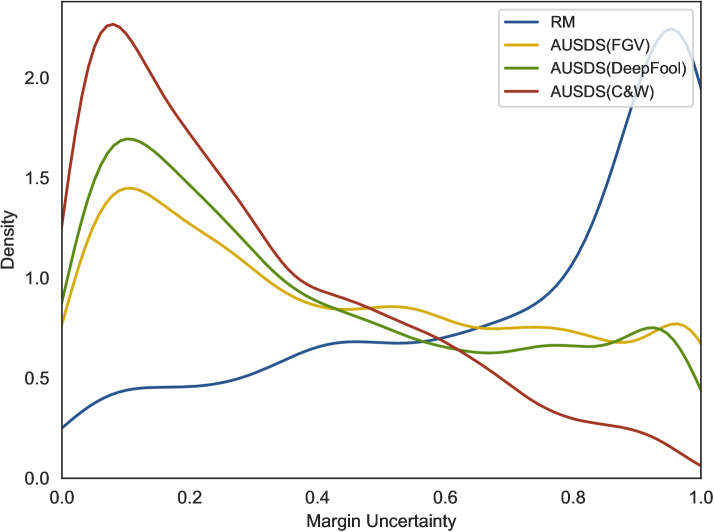
(b) Margin Distribution

Figure 3: The margin of outputs on samples selected by different sampling strategies on SST-5. The margin denotes for differences between the largest and the second-largest output probabilities on different classes. The lower the margin is, the closer the sample is located to the decision boundary. Fig. (a) shows the average margin of each sampling step during training. The margins of samples selected by RM and US on whole unlabeled data are also plotted as references. Fig. (b) shows the margin distribution of samples selected from sampling step 800 to 1000, where the average uncertainty becomes steady. US in Fig. (b) is omitted for better visualization.

4.2 Sampling Effectiveness

AUSDS can achieve higher sampling effectiveness than uncertainty sampling due to the sampling bias problem. The main criteria to evaluate an active learning approach is the sampling effectiveness, namely the model performance with a limited amount of unlabeled data being sampled and labeled. Our AUSDS learning framework is compared with the two baselines using the same amount of labeled data. The limitations are set as 2%, 4%, 6%, 8%, and 10% of all labeled data in each dataset. We only include at most 10% of the whole training data labeled, because active learning focuses on training with a quite limited amount of labeled data by selecting more valuable examples to label. It makes no difference whether to perform active learning or not with enough labeled data available. We believe that with less labeled data, the performance gap, namely the difference of sampling effectiveness is more obvious.

We propose training from scratch setting to better evaluate the sampling effectiveness, in which models are trained from scratch using the labeled data sampled by different approaches with various labeled data sizes. We argue that simply training the model until convergence after each sampling step, which we call continuous training setting, can easily induce the problem of sampling bias Huang et al. (2010). Biased models in the early training phase lead to worse performance even after more informative samples are given. Thus the performance of models during sampling cannot reflect the real informativeness of selected samples.

The from-scratch training results are shown in Table 3. Our framework outperforms the random baselines consistently because it selects more informative samples for identifying the shape of the decision boundary. Also, it outperforms the common uncertainty sampling in most cases with the same labeled data size limits because the frequent sampling processes in our approach alleviate the sampling bias issue. Uncertainty sampling suffers the sampling bias problem because of frequent variation of the decision boundary in the early phase of training, which results in ineffective sampling. The decision boundary is merely determined by a small number of labeled examples in the early phase. And the easily biased decision boundary may lead to the sampling of high uncertainty samples given the current model state but not that representative to the whole unlabelled data. With the overall results on the five standard benchmarks of 2 NLP tasks, we observe that our AUSDS can achieve better sampling effectiveness with DeepFool for sequence classification and FGV for sequence labeling. The results of CW are also included for completeness and comparison.

To prove that our AUSDS framework does not heavily depend on BERT, we conduct experiments on SST-2 with ELMo as the encoder, which has a different network structure. The results in Table  4 show that in this setting, our AUSDS framework still achieves higher sampling effectiveness, while the original uncertainty sampling gets stuck in a more severe sampling bias problem. The results in this experiment can also be evidence of the generalization ability of our framework to other pre-trained LM encoding space.

4.3 Computational Efficiency

AUSDS is computationally more efficient than uncertainty sampling. Our AUSDS is computationally efficient enough to be performed at batch-level, thus achieving real-time effective sampling. The average sampling speeds of different approaches are compared w.r.t. US (Table 2).

We observe that uncertainty sampling can hardly work in a real-time sampling setting because of the costly sampling process. Our AUSDS are more than 10x faster than common uncertainty sampling. The larger the unlabeled data pool is, the more significant the acceleration is. Our framework spends longer computation time, compared with the random sampling baseline, but still fast enough for real-time batch-level sampling. Moreover, the experimental results on Sampling Effectiveness in Sec. 4.2 show that the extra computation for adversarial samples is worthy with obvious performance enhancement on the same amount of labeled data.

4.4 Samples Uncertainty

AUSDS can actually select examples with higher uncertainty. We plot the margins of outputs of samples selected with different sampling strategies on SST-5 in Fig. 3. We use margin as the measurement of the distance to the decision boundary. Lower margins indicate positions closer to the decision boundary. As shown in Fig. 3(a), the samples selected by our AUSDS with different attack approaches achieve lower average margins during sampling. Samples from step 800 to 1000 are collected to estimate the margin distribution, as shown in Fig. 3(b). It is shown that our AUSDS has better capability to capture the samples with higher uncertainty as their margin distributions are more to the left. The uncertainty sampling performed on the whole unlabeled data gets the most uncertain samples. However, it is very time-consuming and can not be applied frequently.

In short, AUSDS achieves better sampling effectiveness in comparison with US because the more efficient batch-level sampling alleviates the problem of sampling bias. Adversarial attacks can be an effective way to find critical data points near the decision boundary.

5 Conclusion

Uncertainty sampling is an effective way of reducing the labeled data size in sentence learning. But uncertainty sampling of high latency may lead to an ineffective sampling problem. In this study, we propose adversarial uncertainty sampling in discrete space for active sentence learning to address the ineffective sampling problem. The proposed AUSDS is more efficient than traditional uncertainty sampling by leveraging adversarial attacks and projecting discrete sentences into pre-trained LM space. Experimental results on five datasets show that the proposed approach outperforms strong baselines in most cases, and achieve better sampling effectiveness.

References

- Altman (1992) Naomi S Altman. 1992. An introduction to kernel and nearest-neighbor nonparametric regression. The American Statistician, 46(3):175–185.
- Berger et al. (1996) Adam L Berger, Vincent J Della Pietra, and Stephen A Della Pietra. 1996. A maximum entropy approach to natural language processing. Computational linguistics, 22(1):39–71.
- Biggio et al. (2013) Battista Biggio, Igino Corona, Davide Maiorca, Blaine Nelson, Nedim Šrndić, Pavel Laskov, Giorgio Giacinto, and Fabio Roli. 2013. Evasion attacks against machine learning at test time. In Joint European conference on machine learning and knowledge discovery in databases, pages 387–402. Springer.
- Carlini and Wagner (2017) Nicholas Carlini and David Wagner. 2017. Towards evaluating the robustness of neural networks. In 2017 IEEE Symposium on Security and Privacy (SP), pages 39–57. IEEE.
- Deng et al. (2018) Yue Deng, KaWai Chen, Yilin Shen, and Hongxia Jin. 2018. Adversarial active learning for sequences labeling and generation. In IJCAI, pages 4012–4018.
- Devlin et al. (2019) Jacob Devlin, Ming-Wei Chang, Kenton Lee, and Kristina Toutanova. 2019. BERT: Pre-training of deep bidirectional transformers for language understanding. In NAACL HLT 2019 - 2019 Conference of the North American Chapter of the Association for Computational Linguistics: Human Language Technologies - Proceedings of the Conference, page 4171–4186. Association for Computational Linguistics.
- Dolan et al. (2004) Bill Dolan, Chris Quirk, and Chris Brockett. 2004. Unsupervised construction of large paraphrase corpora: Exploiting massively parallel news sources. In Proceedings of the 20th international conference on Computational Linguistics, page 350. Association for Computational Linguistics.
- Ducoffe and Precioso (2018) Melanie Ducoffe and Frederic Precioso. 2018. Adversarial active learning for deep networks: a margin based approach. arXiv preprint arXiv:1802.09841.
- Goodfellow et al. (2015) Ian J Goodfellow, Jonathon Shlens, and Christian Szegedy. 2015. Explaining and harnessing adversarial examples. In 3rd International Conference on Learning Representations, ICLR 2015 - Conference Track Proceedings.
- Hoi et al. (2006) Steven CH Hoi, Rong Jin, and Michael R Lyu. 2006. Large-scale text categorization by batch mode active learning. In Proceedings of the 15th international conference on World Wide Web, pages 633–642. ACM.
- Huang et al. (2010) Sheng-Jun Huang, Rong Jin, and Zhi-Hua Zhou. 2010. Active learning by querying informative and representative examples. In Advances in neural information processing systems, pages 892–900.
- Jain et al. (2010) Prateek Jain, Sudheendra Vijayanarasimhan, and Kristen Grauman. 2010. Hashing hyperplane queries to near points with applications to large-scale active learning. In Advances in Neural Information Processing Systems, pages 928–936.
- Johnson et al. (2019) Jeff Johnson, Matthijs Douze, and Hervé Jégou. 2019. Billion-scale similarity search with GPUs. IEEE Transactions on Big Data.
- Joshi et al. (2009) Ajay J Joshi, Fatih Porikli, and Nikolaos Papanikolopoulos. 2009. Multi-class active learning for image classification. In 2009 IEEE Conference on Computer Vision and Pattern Recognition, pages 2372–2379. IEEE.
- Kurakin et al. (2017) Alexey Kurakin, Ian Goodfellow, and Samy Bengio. 2017. Adversarial examples in the physical world. In 5th International Conference on Learning Representations, ICLR 2017 - Workshop Track Proceedings.
- Lewis and Gale (1994) David D Lewis and William A Gale. 1994. A sequential algorithm for training text classifiers. In SIGIR’94, pages 3–12. Springer.
- Li et al. (2018) Pengcheng Li, Jinfeng Yi, and Lijun Zhang. 2018. Query-efficient black-box attack by active learning. In Proceedings - IEEE International Conference on Data Mining, ICDM, page 1200–1205.
- Moosavi-Dezfooli et al. (2016) Seyed-Mohsen Moosavi-Dezfooli, Alhussein Fawzi, and Pascal Frossard. 2016. Deepfool: A simple and accurate method to fool deep neural networks. In The IEEE Conference on Computer Vision and Pattern Recognition (CVPR).
- Pal et al. (2020) Soham Pal, Yash Gupta, Aditya Shukla, Aditya Kanade, Shirish Shevade, and Vinod Ganapathy. 2020. Activethief: Model extraction using active learning and unannotated public data. In Proceedings of the AAAI Conference on Artificial Intelligence, pages 865–872. AAAI.
- Peters et al. (2018) Matthew E Peters, Mark Neumann, Mohit Iyyer, Matt Gardner, Christopher Clark, Kenton Lee, and Luke Zettlemoyer. 2018. Deep contextualized word representations. In NAACL HLT 2018 - 2018 Conference of the North American Chapter of the Association for Computational Linguistics: Human Language Technologies - Proceedings of the Conference, page 2227–2237. Association for Computational Linguistics.
- Radford et al. (2018) Alec Radford, Karthik Narasimhan, Tim Salimans, and Ilya Sutskever. 2018. Improving language understanding by generative pre-training.
- Rozsa et al. (2016) Andras Rozsa, Ethan M Rudd, and Terrance E Boult. 2016. Adversarial diversity and hard positive generation. In Proceedings of the IEEE Conference on Computer Vision and Pattern Recognition Workshops, pages 25–32.
- Sang and De Meulder (2003) Erik F Tjong Kim Sang and Fien De Meulder. 2003. Introduction to the conll-2003 shared task: Language-independent named entity recognition. In Proceedings of the Seventh Conference on Natural Language Learning at HLT-NAACL 2003.
- Settles (2009) Burr Settles. 2009. Active learning literature survey. Technical report, University of Wisconsin-Madison Department of Computer Sciences.
- Settles and Craven (2008) Burr Settles and Mark Craven. 2008. An analysis of active learning strategies for sequence labeling tasks. In Proceedings of the conference on empirical methods in natural language processing, pages 1070–1079. Association for Computational Linguistics.
- Socher et al. (2013) Richard Socher, Alex Perelygin, Jean Wu, Jason Chuang, Christopher D Manning, Andrew Ng, and Christopher Potts. 2013. Recursive deep models for semantic compositionality over a sentiment treebank. In Proceedings of the 2013 conference on empirical methods in natural language processing, pages 1631–1642.
- Szegedy et al. (2014) Christian Szegedy, Wojciech Zaremba, Ilya Sutskever, Joan Bruna, Dumitru Erhan, Ian Goodfellow, and Rob Fergus. 2014. Intriguing properties of neural networks. In 2nd International Conference on Learning Representations, ICLR 2014 - Conference Track Proceedings.
- Zhang et al. (2015) Xiang Zhang, Junbo Zhao, and Yann LeCun. 2015. Character-level convolutional networks for text classification. In Advances in neural information processing systems, pages 649–657.
- Zhu and Bento (2017) Jia-Jie Zhu and José Bento. 2017. Generative adversarial active learning. arXiv preprint arXiv:1702.07956.