A non-convex regularization approach for stable estimation of loss development factors

Abstract

In this article, we apply non-convex regularization methods in order to obtain stable estimation of loss development factors in insurance claims reserving. Among the non-convex regularization methods, we focus on the use of the log-adjusted absolute deviation (LAAD) penalty and provide discussion on optimization of LAAD penalized regression model, which we prove to converge with a coordinate descent algorithm under mild conditions. This has the advantage of obtaining a consistent estimator for the regression coefficients while allowing for the variable selection, which is linked to the stable estimation of loss development factors. We calibrate our proposed model using a multi-line insurance dataset from a property and casualty insurer where we observed reported aggregate loss along accident years and development periods. When compared to other regression models, our LAAD penalized regression model provides very promising results.

Keywords: Insurance reserving, log-adjusted absolute deviation (LAAD) penalty, loss development, non-convex penalization, robust estimation, variable selection.

1 Introduction

The chain ladder method, as an industry benchmark with theoretical foundation as discussed in Mack, (1993) and Mack, (1999), has been widely used to determine the development pattern of reported or paid claims. Despite its prevalence, we need to address some relevant issues in the estimation of development factors for mature years with this chain ladder method. In general, we expect that cumulative reported loss amount increases through time whereas the magnitude of the development decreases. However, it is possible that loss development patterns with some run-off triangles may not follow these expected patterns since we have only a few data points in the top-right corner and estimation of parameters that depends on those data points becomes unstable, due to triangular or trapezoidal shape of aggregated claim data as mentioned in Renshaw, (1989). Therefore, we need to consider some ways to estimate the development factors for mature years with more stability.

To deal with the aforementioned issue of stable estimation of development factors for mature years, one can apply the regularization method or penalized regression in loss development models. Today, there is a rich literature of using penalization in the regression framework. The first penalization method introduced is ridge regression, developed by Hoerl and Kennard, (1970). By adding an $L_{2}$ penalty term on the least squares, they showed that it is possible to have smaller mean squared error when there is severe multicollinearity in a given dataset. Nevertheless, ridge regression has merely the shrinkage property but not the property of variable selection. To tackle this problem, Tibshirani, (1996) suggested LASSO (least absolute shrinkage and selection operator) using an $L_{1}$ penalty term on the least squares, and showed that this enables us to perform variable selection. This method leads to dimension reduction as well. Despite the simplicity of the proposed method, there has been a great deal of work done to extend the LASSO framework. For example, Park and Casella, (2008) solidified Tibshirani’s work by providing a Bayesian interpretation on LASSO. Although LASSO has the variable selection property, the estimates derived from LASSO regression are inherently biased and may over-shrink the retained variables (Hastie et al.,, 2009, 2015).

There have been some meaningful approaches so that we obtain both variable selection and consistency of estimates. For example, Fan and Li, (2001) proposed smoothly clipped absolute deviation (SCAD) penalty, derived by assuming continuously differentiable penalty function to achieve three properties such as (i) consistency of the estimate as the true value of the parameter increases, (ii) variable selection, and (iii) the continuity of the calculated estimates. Although SCAD penalty has the above-mentioned properties, it naturally leads to a non-convex optimization so that it loses desirable properties of convex optimization problems. Zhang, (2010) proposed minimax concave penalty (MCP), which minimizes the maximum concavity subject to an unbiasedness feature. Moreover, Lee et al., (2010) and Armagan et al., (2013) proposed the log-adjusted absolute deviation (LAAD) penalty, which is derived by imposing a hyperprior distribution on the tuning parameter $\lambda$, as proposed in Park and Casella, (2008). The term “LAAD penalty” has been coined in this paper.

The concept of penalized regression in the actuarial literature is not quite new. Indeed, the well-known Whittaker-Henderson mortality graduation method introduced a penalty to balance fit and smoothness of the observed data. See Chan et al., (1982). Yet there has only been a few relevant other works in the field. Williams et al., (2015) applied the elastic net penalty, which is a combination of $L_{1}$ and $L_{2}$ penalties, on a dataset with over 350 initial covariates to enhance insurance claims prediction. Nawar, (2016) used LASSO for detecting possible interaction between covariates, which are used in claims modeling. Yin and Lin, (2016) used a version of non-convex penalty for efficient estimation of Erlang mixture model with a group medical insurance claims data. Recently, McGuire et al., (2018) proposed the use of $L_{1}$ penalization for stable estimation of loss development factors.

In this paper, we explore the use of LAAD regression that enables us to implement variable selection and to obtain smoothness and stability while maintaining consistency of the estimators. These properties inspired us to apply LAAD penalty in a cross-classified regression model to estimate loss development in claims reserving. We also provide theoretical discussions on the convergence of LAAD penalized models based on the coordinate descent algorithm, and describe sufficient conditions for convergence, which are well-satisified in the applications for claims reserving. In calibrating various competing models, we use data drawn from a property and casualty (P&C) insurer with two lines of business; the claims reported are conveniently expressed as loss triangles. We compare the estimated loss development factors of our proposed model with a straightforward cross-classified model and cross-classified models with LASSO and non-convex penalties, including LAAD. All these models are comparably explained in the section on estimation and prediction; we also discuss the validation measures for comparison purposes. Among these various models, our LAAD regression model performed remarkably well, which produced estimates of loss development factors with reasonable patterns and consistent with a priori knowledge. It also provides more improved prediction of reserve estimates. We additionally examined its usefulness in insurance ratemaking and this is summarized in the appendix.

This paper has been organized as follows. In Section 2, we introduce the construction of the LAAD penalty and provide sufficient condition for the convergence of the coordinate descent algorithm that forms the foundation to calibrate a LAAD regression model. In Section 3, we show the efficacy of the proposed method using a simulation study. In Section 4, we explore possible use of LAAD penalty in insurance claims reserving using an insurer’s dataset with multi-line reported loss triangles. We discuss the results of the estimation and evaluate predictions for the various models examined. We conclude in Section 5.

2 LAAD penalization model and optimization

2.1 Derivation and properties of LAAD penalty

According to Park and Casella, (2008), we may interpret LASSO in a Bayesian framework as follows:

$$Y|\beta\sim N(X\beta,\sigma^{2}I_{n}),\quad\beta_{i}|\lambda\sim\text{Laplace}(0,1/\lambda),$$

where $\beta$ is a vector of size $p$ with each component having a density function $p(\beta_{i}|\lambda)=\frac{\lambda}{2}e^{-\lambda{|\beta_{i}|}}$, for $\beta_{i}\in\mathbb{R}$. According to their specification, we may express the likelihood and the log-likelihood for $\beta$, respectively, as

$$L(\beta|y,X,\lambda)\ \propto\ \exp\left(-\frac{1}{2\sigma^{2}}\left[\sum_{i=1}^{n}(y_{i}-X_{i}\beta)^{2}\right]-\lambda||\beta||_{1}\right)\ \text{and}$$ (1)

$$\ell(\beta|y,X,\lambda)=-\frac{1}{2\sigma^{2}}\left[\sum_{i=1}^{n}(y_{i}-X_{i}\beta)^{2}\right]-\lambda||\beta||_{1}+\text{Constant}.$$

Park and Casella, (2008) suggested two approaches to choose the optimal $\lambda$ in Equation (1). One is the use of point estimate by cross-validation, and the other is the use of a ‘hyperprior’ distribution for $\lambda$.

Now, consider the following distributional assumptions

$$Y|\beta\sim N(X\beta,\sigma^{2}I_{n}),\quad\beta_{j}|\lambda_{j}\sim\text{Laplace}(0,1/\lambda_{j}),\quad\text{and}\quad\lambda_{j}|r\overset{i.i.d.}{\sim}\text{Gamma}(r/\sigma^{2}-1,1).$$

In other words, the hyperprior of $\lambda_{j}$ follows a gamma distribution with density $p(\lambda_{j}|r)=\lambda_{j}^{\frac{r}{\sigma^{2}}-2}e^{-\lambda_{j}}/\Gamma(\frac{r}{\sigma^{2}}-1)$. This implies that we have:

$$L(\beta,\lambda_{1},\ldots,\lambda_{p}|y,X,r)\ \propto\ \exp\left(-\frac{1}{2\sigma^{2}}[\sum_{i=1}^{n}(y_{i}-X_{i}\beta)^{2}]\right)\times\prod_{j=1}^{p}\exp\left(-\lambda_{j}\left[|\beta_{j}|+1\right]\right)\lambda_{j}^{\frac{r}{\sigma^{2}}-1},$$ (2)

$$L(\beta|y,X,r)=\int L(\beta,\lambda|y,X,r)d\lambda\ \propto\ \exp\left(-\frac{1}{2\sigma^{2}}[\sum_{i=1}^{n}(y_{i}-X_{i}\beta)^{2}]\right)\times\prod_{j=1}^{p}\left(1+|\beta_{j}|\right)^{-\frac{r}{\sigma^{2}}},$$

$$\ell(\beta|y,X,r)=-\frac{1}{2\sigma^{2}}\left(\sum_{i=1}^{n}(y_{i}-X_{i}\beta)^{2}+2r\sum_{j=1}^{p}\log(1+|\beta_{j}|)\right)+\text{Constant}.$$

As a result, the log-likehood in Equation (2) allows us to have the following formulation of our penalized least squares problem. This gives rise to what we call the log-adjusted absolute deviation (LAAD) penalty function:

$$||\beta||_{L}=\sum_{j=1}^{p}\log(1+|\beta_{j}|),$$

so that

$$\hat{\beta} =\ \mathop{\mathrm{missing}}{argmin}_{\beta}\frac{1}{2}||y-X\beta||^{2}+r\sum_{j=1}^{p}\log(1+|\beta_{j}|).$$

Such derivation of LAAD penalty has been used in the statistical literature including an application on non-convex paths (Mazumder et al.,, 2011) and health care (Wang et al.,, 2019).

To further understand the characteristics of a model with LAAD penalty, consider a simple example when $p=1$ and $||X||=1$. In this case, optimization of $\ell$ in Equation (2) is reduced to a univariate case so that it is enough to solve the following:

$$\hat{\theta}_{j}=\mathop{\mathrm{missing}}{argmin}_{\theta_{j}}\frac{1}{2}(z_{j}-\theta_{j})^{2}+r\log(1+|\theta_{j}|),$$ (3)

where $z=X^{\prime}y$.

Theorem 1.

Let us set $\ell(\theta|r,z)=\frac{1}{2}(z-\theta)^{2}+r\log(1+|\theta|)$. Then the corresponding minimizer will be given as $\hat{\theta}=\theta^{*}\cdot\mathbbm{1}_{\{|z|\geq z^{*}(r)\vee r\}}$, where

$$\theta^{*}=\frac{1}{2}\left[z+\text{sgn}(z)\left(\sqrt{(|z|-1)^{2}+4|z|-4r}-1\right)\right],$$

and $z^{*}(r)$ is the unique solution of

$$\Delta(z|r)=\frac{1}{2}(\theta^{*})^{2}-\theta^{*}z+r\log(1+|\theta^{*}|)=0.$$

Proof.

See Appendix A. ∎

Note that $\theta^{*}=\frac{z}{2}+\text{sgn}(z)\left[\frac{\sqrt{(|z|+1)^{2}-4r}-1}{2}\right]\simeq\frac{z}{2}+\text{sgn}(z)\left[\frac{(|z|+1)-1}{2}\right]=z$ when $|z|$ is large enough, which means $\theta^{*}$ converges to $z$ when $|z|\rightarrow\infty$. Therefore, by using LAAD penalty, we obtain an optimizer which has properties of variable selection, consistency, and continuity as demonstrated in Armagan et al., (2013).

Figure 1 provides graphs that describe the behavior of the obtained optimizer derived with different penalization. The first graph is the behavior of the optimizer derived with $L_{2}$ penalty, which is also called ridge regression. In this case, as previously alluded, it has no variable selection property but it only shrinks the magnitude of the estimates. The second graph is the behavior of the optimizer derived with $L_{1}$ penalty, which is the basic LASSO. In this case, we see that although it has the variable selection property (if value of $\beta$ is small enough, then $\hat{\beta}$ becomes 0), the discrepancy between the true $\beta$ and $\hat{\beta}$ remains constant even when the true $|\beta|$ is very big. Finally, the third graph shows the behavior of the optimizer derived with the proposed LAAD penalty. One can see that not only does the given optimizer have the variable selection property, but also $\hat{\beta}$ converges to $\beta$ as $|\beta|$ increases.

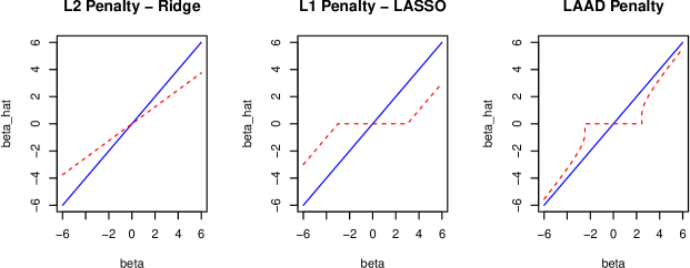
Figure 1: Estimate behavior for several penalty functions

Figure 2 illustrates the constraint regions implied by each penalty. It is well known that the constraint regions defined by $L_{2}$ penalization is a $p$-dimensional circle, whereas the constraint regions defined by $L_{1}$ penalization is a $p$-dimensional diamond. We observe that in both cases of $L_{2}$ and $L_{1}$ penalization, the constraint regions are convex, which implies that we entertain the properties of convex optimization. In the case of the constraint implied by LAAD penalty, the region is non-convex, which is inevitable to obtain both consistency of the estimates and variable selection property as in the case of Bridge or $L_{q}$ penalization with $q\in(0,1)$. However, it is known that there is no closed form solution in the univariate case of $L_{q}$ penalized linear regression when $q\in(0,1)$ (Knight and Fu,, 2000) so that it is difficult to apply $L_{q}$ penalty $(0<q<1)$ on high-dimensional problems with the coordinate descent algorithm, let alone analyze convergence.

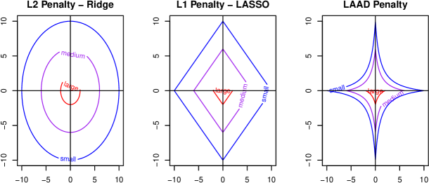
Figure 2: Constraint regions for several penalties

It is also possible to compare the behavior of LAAD penalty with SCAD penalty and MCP. According to Fan and Li, (2001) and Zhang, (2010), one can write down the penalty functions (and their derivatives) in the univariate case, assuming $\theta\geq 0$, as follows:

$$p_{LASSO}(\theta;\lambda)=\lambda\theta,\quad p^{\prime}_{LASSO}(\theta;\lambda)=\lambda,$$ (4)

$$p_{MCP}(\theta;\lambda,\gamma)=\int_{0}^{\theta}\lambda(1-x/\gamma\lambda)_{+}dx,\quad p^{\prime}_{MCP}(\theta;\lambda,\gamma)=\lambda(1-\theta/\gamma\lambda)_{+},$$

$$p^{\prime}_{SCAD}(\theta;\lambda,a)=\lambda\{I(\theta\leq\lambda)+\frac{(a\lambda-\theta)_{+}}{(a-1)\lambda}I(\theta>\lambda)\},\ \text{and}$$

$$p_{LAAD}(\theta;\lambda)=\lambda\log(1+\theta),\quad p^{\prime}_{LAAD}(\theta;\lambda)=\lambda\left(\frac{1}{1+\theta}\right).$$

From above, it is straightforward to see that

$$\lim_{\theta\rightarrow\infty}p^{\prime}_{SCAD}(\theta;\lambda,a)=\lim_{\theta\rightarrow\infty}p^{\prime}_{MCP}(\theta;\lambda,\gamma)=\lim_{\theta\rightarrow\infty}p^{\prime}_{LAAD}(\theta;\lambda)=0.$$

This implies that the marginal effect of penalty converges to 0 as the value of $\theta$ increases and hence, the magnitude of distortion on the estimate becomes negligible as the true coefficient gets larger when we use either SCAD, MCP, or LAAD penalty. However, we see that $\lim_{\theta\rightarrow\infty}p^{\prime}_{LASSO}(\theta;\lambda)=\lambda$, which means that the magnitude of distortion on the estimate is the same even in the case when the true coefficient is very large.

On the other hand, if we let $\theta$ go to 0, one can see that

$$\lim_{\theta\rightarrow 0+}p^{\prime}_{SCAD}(\theta;\lambda,a)=\lim_{\theta\rightarrow 0+}p^{\prime}_{MCP}(\theta;\lambda,\gamma)=\lim_{\theta\rightarrow 0+}p^{\prime}_{LAAD}(\theta;\lambda)=\lim_{\theta\rightarrow 0+}p^{\prime}_{LASSO}(\theta;\lambda)=\lambda,$$

which implies that for SCAD, MCP, and LAAD penalty, the magnitude of penalization is the same as LASSO when the true value of $\theta$ is very small. Therefore, we verify that SCAD, MCP, and LAAD penalties have the same property of variable selection as LASSO, when the true $\theta$ is small enough.

To summarize, it can be deduced that the use of LAAD penalty rewards sparsity more so than LASSO penalty. Although the overall degree of penalization is determined by cross-validation in both cases, penalization is evenly applied on all coefficients in the case of LASSO, while penalization is more severe for smaller coefficients in the case of LAAD. The landscape of penalization can be quite different from each other. Therefore, use of LAAD penalized regression results in less shrinkage on the estimated coefficients but more variable selection.

2.2 Implementation in general case and convergence analysis

Estimating parameters from given penalized least squares is an optimization problem. Since an analytic solution is obtained in the case of univariate penalized least squares, one can implement an algorithm for optimization. For example, in obtaining $\hat{\beta}$ in the multivariate case, we may apply a coordinate descent algorithm proposed by Luo and Tseng, (1992), which starts with an initial estimate and then successively optimizes along each coordinate or blocks of coordinates. The algorithm is explained in detail as follows:

Algorithm 1 A coordinate descent algorithm for LAAD penalty

  Input: Training dataset $X=(X_{1},\ldots,X_{p}),\,y$, initial parameter $\beta^{(0)}=\hat{\beta}^{OLS}$, a function $\hat{\theta}$ defined on Theorem 1, regularization parameter $r$, tolerance $\epsilon>0$.

1:  while $||\beta^{(t)}-\beta^{(t-1)}||>\epsilon$ :

2:   Residual $\leftarrow y-\sum_{j=1}^{p}X_{j}\beta^{(t-1)}$

3:   For $j$ in $1:p$ :

4:    Residual $\leftarrow$ Residual + $X_{j}\beta_{j}^{(t-1)}$

5:    $z_{(t-1,j)}\leftarrow X_{j}^{\top}$Residual

6:    $\beta_{(j)}^{(t)}\leftarrow\hat{\theta}(z_{(t-1,j)},r)$

7:    Residual $\leftarrow$ Residual - $X_{j}\beta_{j}^{(t)}$

8:  Output: $\hat{\beta}^{LAAD}=\beta^{(t)}$

Interestingly, although the use of LAAD penalty has been explored in the statistics literature, a thorough analysis on the convergence of a coordinate descent algorithm for LAAD regression model is still scarce. Mazumder et al., (2011) found that application of a coordinate descent algorithm to LAAD penalized model “can produce multiple limit points (without converging) - creating statistical instability in the optimization procedure”, though they did not provide a sufficient condition which assures statistical stability in the optimization procedure. In this regard, here we provide a sufficient condition so that the coordinate descent algorithm converges with our optimization problem. To prove convergence, we need to introduce the concepts of quasi-convex and hemivariate. A function is hemivariate if a function is not constant on any interval which belongs to its domain. A function $f$ is quasi-convex if

$$f(x+\lambda d)\leq\max\{f(x),\,f(x+d)\},\ \text{for all }x,d\text{ and }\lambda\in[0,1].$$

An example of a function which is quasi-convex and hemivariate is $f(x)=\log(1+|x|)$.

The following lemma is useful for obtaining a sufficient condition that our optimization problem converges with the coordinate descent algorithm.

Lemma 1.

Suppose a function $\ell:\mathbb{R}^{p}\rightarrow\mathbb{R}$ is defined as follows:

$$\ell(\beta_{1},\ldots,\beta_{p})=\frac{1}{2}||y-X\beta||^{2}+r\sum_{j=1}^{p}\log(1+|\beta_{j}|)$$

and $||X_{j}||=1$ for all $j=1,\ldots,p$. If $r\leq 1$, then $\ell_{j}:\beta_{j}\mapsto\ell(\beta_{1},\ldots,\beta_{p})$ is both quasi-convex and hemivariate for all $j=1,\ldots,p$.

Proof.

See Appendix B. ∎

Note that the sum of quasi-convex functions may not be quasi-convex. Therefore, although both $||y-X\beta||^{2}$ and $\log(1+|\beta_{j}|)$ are quasi-convex functions as functions of $\beta_{j}$ on $\mathbb{R}$, it does not assure that $\ell(\beta_{1},\ldots,\beta_{p})$ is a quasi-convex function for each coordinate. Intuitively, a continuous function on $\mathbb{R}$ is quasi-convex if and only if it has unique local minimum. In this regard, $f(x)=\log(1+|x|)+0.01(10-x)^{2}$ is a quasi-convex function since

$$f^{\prime}(x)=\begin{cases}\frac{1}{1+x}+0.02(x-10)>0;&x>0,\\ \frac{-1}{1-x}+0.02(x-10)<0;&x<0,\\ \end{cases}$$

and $f(x)$ has unique local (indeed, global) minimum at $x=0$.

However, if $g(x)=7\log(1+|x|)+(3-x)^{2}$, then $g(x)$ is not quasi-convex since such function has two local minima, $0$ and $1+1/\sqrt{2}$. Figure 3 provides visualization of these two examples.

Figure 3: An example of quasi-convex function and non-quasi-convex function

Therefore, $r\leq 1$ is the critical condition in the proof of Lemma 1, and it leads to the following theorem which assures the convergence of coordinate descent algorithm for LAAD regression models.

Theorem 2.

If $||X_{j}||=1$ for all $j=1,\ldots,p$ and $r\leq 1$, then the solution from the coordinate descent algorithm with function $l:\mathbb{R}^{p}\rightarrow\mathbb{R}$ converges to $\hat{\beta}$ where

$$\hat{\beta} =\ \mathop{\mathrm{missing}}{argmin}_{\beta}\frac{1}{2}||y-X\beta||^{2}+r\sum_{j=1}^{p}\log(1+|\beta_{j}|).$$

Proof.

According to Theorem 5.1 of Tseng, (2001), it suffices to show that 1) $||y-X\beta||^{2}$ is continuous on $\mathbb{R}^{p}$, 2) $\log(1+|\beta_{j}|)$ is lower semicontinuous, and 3) $\ell_{j}:\beta_{j}\mapsto l(\beta_{1},\ldots,\beta_{p})$ is quasi-convex and hemivariate. 1) and 2) are obvious and 3) could be shown from Lemma 1. ∎

As shown in Theorem 2, the applicability of estimation with LAAD penalty heavily depends on the range of tuning parameter $r$, which assures convergence of the algorithm if $r\leq 1$. For example, when LAAD penalization is applied to the stable estimation of loss development factor, it is known that the estimated loss development factor for later development years are usually quite low so it is innocuous to impose such condition, which is confirmed in Section 4.

Finally, it is possible to try extending LAAD regression given in (2) in various directions. For example, one can consider

$$||Y-X\beta||^{2}+r\sum_{j=1}^{p}\log(1+|\beta_{j}|^{q}),$$

where $q\in(0,\infty)$ controls the behavior of penalty. If $q=2$, then we expect the behavior of penalty function is very similar to that of ridge regression for small coefficients. Indeed, we can draw a penalty solution as in Figures 1 and 2 for this case and confirm that while it preserves the shrinkage property, it is unable to perform variable selection. If $q\in(0,1)$, then it is natural to expect stronger variable selection than LAAD, but optimization will be more challenging than that of LAAD, as in usual Bridge regression with $q\in(0,1)$. Further, LAAD penalized regression can be extended to other distributions so that one optimizes the following penalized likelihoods from the GLM family of the form:

$$\ell\left(g(X\beta);y\right)+r\sum_{j=1}^{p}\log(1+|\beta_{j}|),$$

where $g$ is the link function.

However, it should be noted that such forms of objective functions are highly non-convex so that the theoretical results from Theorem 2 do not necessarily hold and corresponding convergence analysis should be performed on a case-by-case. To illustrate, consider a random variable $Y\in\{0,1\}$ that is distributed as $\mathbb{P}(Y=1|x)=\dfrac{e^{\beta_{0}+x\beta_{1}}}{1+e^{\beta_{0}+x\beta_{1}}}$; we observe $\mathbf{y}=(0,1)$ and $\mathbf{x}=(1,0)$. In this case, the log-likelihood with LAAD penalty when $r=1$ is given as $\ell(\beta_{0},\beta_{1})=\beta_{0}-\ln(1+e^{\beta_{0}+\beta_{1}})+\ln(1+|\beta_{1}|)$. In this case, one can easily check that $\ell_{1}:\beta_{1}\rightarrow\ell(\beta_{0},\beta_{1})$ may not be a quasi-convex function even if $r\leq 1$ and $||X||=1$ since $\ell_{1}(x+\lambda d)>-\ln 2>\max\{\ell_{1}(x),\,\ell_{1}(x+d)\}$, when $x=0,d=1,\lambda=0.5$, and $\beta_{0}=0$.

3 Simulation study

In this section, we conduct a simulation study so as to show the novelty of the proposed method. Suppose we have the following nine available covariates $(X_{1},\ldots,X_{9})$ and response variable $y$ which are generated as follows:

$$X_{1}\sim\mathcal{N}(5,1),\ X_{2}\sim\mathcal{N}(-2,1),\ X_{3}\sim\mathcal{N}(1,4),\ X_{4}\sim\mathcal{N}(3,4),\ X_{5}\sim\mathcal{N}(0,4),$$

$$X_{6}\sim\mathcal{N}(0,9),\ X_{7}\sim\mathcal{N}(-3,4),\ X_{8}\sim\mathcal{N}(2,1),\ X_{9}\sim\mathcal{N}(3,1),\ \epsilon\sim\mathcal{N}(0,1),$$

$$y=-X_{1}+X_{2}+X_{3}-X_{4}+X_{5}-X_{6}+X_{7}+X_{8}-X_{9}-10X_{1}X_{6}+X_{2}X_{3}+0.1X_{3}X_{4}-0.01X_{4}X_{6}+\epsilon,$$

so that the simulation scheme can incorporate possible interactions in the model (while the model is still sparse enough) for which the magnitude effects vary. One can check that if a regression model is calibrated using $(X_{1},X_{2},\ldots,X_{9})$, then the estimated regression coefficients are all significant. However, even if all covariates are significant by themselves, omission of effective interaction terms can lead to bias in the estimated coefficients and subsequently lack of fit as illustrated in Figure 4. In Figure 4, reduced model means a linear model fitted only with $(X_{1},\,X_{2},\,\ldots,\,X_{9})$, while true model is a linear model fitted with $(X_{1},\,X_{2},\,\ldots,\,X_{9},\,X_{1}X_{6},\,X_{2}X_{3},\,X_{3}X_{4},\,X_{4}X_{6})$.

Figure 4: QQplots for reduced model and true model

On the other hand, including every interaction terms also may end up with an inferior model since it may accumulate noise in the estimation, which leads to larger variances in the estimates. As elaborated in James et al., (2013), the mean squared error (MSE) of a predicted value under a linear model is determined by both the variance and the squared bias of the estimated regression coefficients as follows:

$${\mathbb{E}}\left[y_{0}-\hat{f}(x_{0})\right]^{2} =Var(\hat{f}(x_{0}))+[\text{Bias}(\hat{f}(x_{0}))]^{2}+Var(\epsilon)$$ (5)

$$=(x_{0})^{\prime}\left[Var(\hat{\beta})+\text{Bias}(\hat{\beta})^{2}\right](x_{0})+\sigma^{2}.$$

As shown in Equation (5), prediction performance of a new observation from out-of-sample validation set, $y_{0}$, can be determined by the stochastic error, $\sigma^{2}$, and the parameter error, $MSE(\hat{\beta})=Var(\hat{\beta})+\text{Bias}(\hat{\beta})^{2}$, in a linear predictive model. Henceforth, it suffices to evaluate the estimation performance of $\hat{\beta}$ to assess the predictive ability of a model since the stochastic error is irreducible and independent of the predictive model.

Here we also note that by including fewer variables in our model with the variable selection, we may get lower $Var(\hat{\beta})$. However, it could increase $[\text{Bias}(\hat{\beta})]^{2}$ due to omitted variable bias (i.e., if a variable has been selected out) or inherent bias of the estimated value because of the penalization. Therefore, it implies that if most of the original variables are significant so that the magnitude of the bias is too high, then the benefit of a reduced $Var(\hat{\beta})$ is compensated by a higher $[\text{Bias}(\hat{\beta})]^{2}$. In this regard, variable selection should be performed carefully to make a balance between the bias and variance and get better prediction with lower mean squared error.

To show the novelty of our proposed penalty function, we first obtain 100 replications of simulated samples $(X_{1},\,X_{2},\,\ldots,\,X_{9},\,y)$ with sample sizes $100,300$, and $1000$ to account for the impact of ratio $p/n$ on estimation and estimate the regression coefficients based on the following seven models:

• Full model: a linear model fitted with $(X_{1},\,X_{2},\,\ldots,\,X_{9})$ and every possible interaction among them,

• Reduced model: a linear model fitted only with $(X_{1},\,X_{2},\,\ldots,\,X_{9})$,

• Best model: Full model regularized with $L_{0}$ penalty (forward feature selection),

• LASSO model: Full model regularized with $L_{1}$ penalty,

• MCP model: Full model regularized with MC penalty,

• SCAD model: Full model regularized with SCAD penalty,

• LAAD model: Full model regularized with LAAD penalty.

All these models were calibrated using the computational routines from the statistical software R. For Full model and Reduced model, the basic lm function was used. Best model was fitted using regsubsets function in leaps package (Lumley,, 2013). LASSO model was fitted using glmnet in Friedman et al., (2009). MCP model and SCAD model were fitted using plus package (Zhang and Melnik,, 2009). There is no standard package to solve the LAAD model.

To evaluate the estimation results under each model, we introduce the following metrics, which measure the discrepancy between the true coefficients and estimated coefficients under each model.

$$\text{Bias for }\beta_{j} =\frac{1}{100}\sum_{s=1}^{100}(\beta_{j}-\hat{\beta}_{j(s)}),\ \ \text{Root Mean Squared Error for }\beta_{j}=\sqrt{\frac{1}{100}\sum_{s=1}^{100}(\beta_{j}-\hat{\beta}_{j(s)})^{2}},$$

where $\beta_{j}$ means the true value of $j^{th}$ coefficient and $\hat{\beta}_{j(s)}$ refers to the estimated value of $j^{th}$ coefficient with $s^{th}$ simulated sample. According to Table 1, Full model is most favored in terms of the bias of estimated coefficients, which is reasonable since ordinary least square (OLS) estimator is unbiased. However, one can see MSEs of estimated coefficients under Full model tend to be greater than those of LAAD model so that LAAD model is expected to provide better estimation, especially when $n$, the sample size, is relatively smaller compared to $p$, the number of covariates. It is also observed that estimation results with Reduced model is quite poor whereas the performance of Best model and LAAD model are the best.

Table 1: Summary of estimation

	Bias							RMSE
	Full	Reduced	Best	LASSO	MCP	SCAD	LAAD	Full	Reduced	Best	LASSO	MCP	SCAD	LAAD
Sample size: n=1000
x1	-0.006	0.107	-0.001	-0.275	-0.714	-0.713	0.000	0.082	0.977	0.042	0.526	0.747	0.743	0.030
x2	-0.020	1.080	-0.002	0.490	-0.938	-0.916	-0.002	0.165	1.399	0.056	0.930	0.970	0.957	0.040
x3	-0.011	-1.639	-0.014	-0.492	-0.970	-0.960	-0.027	0.099	1.713	0.086	0.552	0.985	0.978	0.054
x4	0.003	0.164	-0.003	-0.044	0.921	0.910	0.005	0.116	0.438	0.055	0.406	0.959	0.953	0.024
x5	0.012	-0.048	0.006	-0.178	-0.133	-0.036	-0.014	0.123	0.512	0.042	0.241	0.363	0.131	0.030
x6	-0.004	-50.062	-0.024	-0.265	0.968	0.989	0.035	0.088	50.066	0.071	0.284	0.985	0.995	0.079
x7	0.004	-0.055	-0.001	-0.231	-0.941	-0.896	-0.006	0.114	0.471	0.050	0.478	0.966	0.941	0.022
x8	-0.003	0.045	-0.001	-0.250	-0.953	-0.966	-0.084	0.180	0.822	0.135	0.746	0.975	0.980	0.246
x9	0.012	0.232	0.018	0.636	0.940	0.979	0.053	0.148	1.054	0.091	0.809	0.969	0.986	0.166
‘x1 : x6‘	0.001	10.000	0.001	0.045	-0.189	-0.194	-0.009	0.012	10.000	0.012	0.048	0.193	0.195	0.016
‘x2 : x3‘	-0.001	-1.000	-0.001	-0.074	-0.206	-0.255	-0.014	0.016	1.000	0.016	0.079	0.248	0.312	0.021
‘x3 : x4‘	0.001	-0.100	0.001	0.004	-0.055	-0.074	-0.004	0.008	0.100	0.008	0.012	0.084	0.088	0.008
‘x4 : x6‘	0.000	0.010	0.006	0.007	0.008	0.010	0.005	0.005	0.010	0.009	0.008	0.011	0.010	0.006
Sample size: n=300
x1	-0.006	0.107	-0.001	-0.275	-0.714	-0.713	0.000	0.176	1.606	0.109	0.787	0.767	0.757	0.127
x2	-0.020	1.080	-0.002	0.490	-0.938	-0.916	-0.002	0.370	1.900	0.328	1.308	0.974	0.990	0.377
x3	-0.011	-1.639	-0.014	-0.492	-0.970	-0.960	-0.027	0.221	1.905	0.166	0.599	0.995	0.990	0.133
x4	0.003	0.164	-0.003	-0.044	0.921	0.910	0.005	0.216	0.936	0.109	0.648	0.944	0.958	0.046
x5	0.012	-0.048	0.006	-0.178	-0.133	-0.036	-0.014	0.259	0.903	0.116	0.395	0.594	0.409	0.120
x6	-0.004	-50.062	-0.024	-0.265	0.968	0.989	0.035	0.171	49.967	0.111	0.390	0.990	0.995	0.177
x7	0.004	-0.055	-0.001	-0.231	-0.941	-0.896	-0.006	0.214	0.872	0.160	0.681	0.934	0.945	0.060
x8	-0.003	0.045	-0.001	-0.250	-0.953	-0.966	-0.084	0.397	1.873	0.490	1.332	0.975	0.985	0.540
x9	0.012	0.232	0.018	0.636	0.940	0.979	0.053	0.326	1.822	0.339	1.016	0.989	0.989	0.260
‘x1 : x6‘	0.001	10.000	0.001	0.045	-0.189	-0.194	-0.009	0.023	10.000	0.020	0.065	0.191	0.193	0.034
‘x2 : x3‘	-0.001	-1.000	-0.001	-0.074	-0.206	-0.255	-0.014	0.033	1.000	0.032	0.093	0.265	0.312	0.036
‘x3 : x4‘	0.001	-0.100	0.001	0.004	-0.055	-0.074	-0.004	0.016	0.100	0.016	0.022	0.081	0.089	0.018
‘x4 : x6‘	0.000	0.010	0.006	0.007	0.008	0.010	0.005	0.012	0.010	0.011	0.011	0.014	0.013	0.009
Sample size: n=100
x1	-0.039	0.128	-0.158	-0.168	-0.703	-0.619	0.015	0.437	3.051	0.350	1.401	0.838	0.827	0.298
x2	-0.040	1.191	-0.305	0.170	-0.910	-0.830	-0.305	0.923	3.366	0.677	2.148	0.982	0.997	0.584
x3	0.001	-1.705	-0.119	-0.572	-0.976	-0.957	-0.377	0.613	2.302	0.490	0.762	0.991	0.980	0.585
x4	0.042	0.326	0.122	0.355	0.878	0.867	0.097	0.523	1.601	0.385	0.819	0.942	0.937	0.343
x5	-0.149	0.078	-0.203	-0.520	-0.730	-0.560	-0.330	0.612	1.568	0.507	0.702	0.856	0.745	0.516
x6	0.046	-49.945	0.042	-0.588	1.000	1.000	0.135	0.353	49.981	0.310	0.826	1.000	1.000	0.570
x7	0.038	0.000	-0.112	-0.177	-0.891	-0.868	-0.129	0.558	1.651	0.383	1.088	0.946	0.931	0.370
x8	0.043	0.155	-0.621	-0.489	-0.978	-0.983	-0.606	0.910	3.275	0.888	2.066	0.987	0.990	0.751
x9	0.024	0.145	0.332	0.392	0.856	0.806	0.232	0.771	3.355	0.677	1.576	0.974	0.981	0.528
‘x1 : x6‘	-0.006	10.000	-0.011	0.111	-0.180	-0.181	-0.019	0.053	10.000	0.047	0.147	0.184	0.185	0.111
‘x2 : x3‘	0.004	-1.000	-0.008	-0.119	-0.222	-0.213	-0.043	0.072	1.000	0.063	0.157	0.291	0.300	0.080
‘x3 : x4‘	0.000	-0.100	-0.005	-0.008	-0.020	-0.048	-0.007	0.042	0.100	0.045	0.043	0.090	0.088	0.036
‘x4 : x6‘	0.002	0.010	0.006	0.007	0.000	0.007	0.001	0.026	0.010	0.016	0.020	0.027	0.019	0.016

Besides the values of estimated coefficients, it is also of interest to capture correct degree of sparsity in a model with the following measures:

$$\text{Mean }L_{1}\text{ norm difference} =\frac{1}{100}\sum_{s=1}^{100}\sum_{j=1}^{p}|\beta_{j}-\hat{\beta}_{j(s)}|,$$

$$\text{Mean }L_{0}\text{ norm difference} =\frac{1}{100}\sum_{s=1}^{100}\sum_{j=1}^{p}\mathbbm{1}_{\{\beta_{j}=0\neq\hat{\beta}_{j(s)}\text{ or }\beta_{j}\neq 0=\hat{\beta}_{j(s)}\}}.$$

Table 2 shows how LAAD model captures the sparsity of the true model correctly. Again, it is shown that the estimation efficiency deteriorates as we have smaller sample in all models but one can see that LAAD model and Best model show the smallest mean $L_{1}$ and $L_{0}$ norm differences, respectively, while Full model fails to capture the sparsity of the true model. Therefore, this simulation supports the assertion that LAAD penalty can be utilized in practice with better performance in a reasonable amount of computation time relative to other penalization methods.

Table 2: Norm differences and computation times for each model

	Full	Reduced	Best	LASSO	MCP	SCAD	LAAD
Mean L1 norm differences
$n=1000$	2.325	68.429	1.578	5.961	10.048	9.888	1.450
$n=300$	3.750	71.584	2.624	8.205	10.381	10.216	2.481
$n=100$	7.657	78.160	5.544	12.607	11.066	10.693	5.224
Mean L0 norm differences
$n=1000$	31.000	5.000	6.550	19.930	12.900	12.410	4.510
$n=300$	31.000	5.000	7.620	22.290	13.910	13.240	9.100
$n=100$	31.000	5.000	10.820	23.610	15.410	15.330	13.790
Average computation times
$n=1000$	0.007	0.002	0.009	0.087	0.415	0.439	0.090
$n=300$	0.005	0.002	0.008	0.071	0.331	0.349	0.040
$n=100$	0.005	0.002	0.007	0.067	0.296	0.229	0.024

4 Empirical application: loss development methods

Claims reserving is a key task to assure solvency of insurer. This section demonstrates an empirical application of using LAAD regression and in spite of the non-convex nature of the penalty, it has the promise of producing stable and smooth estimates of loss development factors, as well as reasonable estimates of insurance claim reserves. For additional application to insurance ratemaking, please see appendix.

4.1 Data characteristics

A dataset from ACE Limited 2011 Global Loss Triangles is used for our empirical analysis which is shown in Tables 3 and 4. This dataset is a summarization of two lines of insurance business that include General Liability and Other Casualty in the form of reported claim triangles.

The given dataset can also be expressed as:

$$\mathcal{D}_{1:I}=\{Y_{ij}^{(n)}:1\leq i\leq I\,\text{ and }\,1\leq j\leq\min(I,I+1-i),\,n=1,2\},$$ (6)

where $Y^{(n)}_{ij}$ refers to the reported claim for $n^{th}$ line of insurance business in $i^{th}$ accident years with $j^{th}$ development lag. Note that $I=10$ in our case and these are displayed in upper-left parts of Tables 3 and 4.

Based on the reported claim data (upper triangle), an insurance company needs to predict the ultimate claims (lower triangle) described as follows:

$$\mathcal{D}_{I+k}=\{Y_{ij}^{(n)}:1+k\leq i\leq I\,\text{ and }\,j=I+1+k-i,\,n=1,2\}.$$ (7)

Table 3: Reported claim triangle for General Liability

	DL 1	DL 2	DL 3	DL 4	DL 5	DL 6	DL 7	DL 8	DL 9	DL 10
AY 1	87,133	146,413	330,129	417,377	456,124	556,588	563,699	570,371	598,839	607,665
AY 2	78,132	296,891	470,464	485,708	510,283	568,528	591,838	662,023	644,021	654,481
AY 3	175,592	233,149	325,726	449,556	532,233	617,848	660,776	678,142	696,378
AY 4	143,874	342,952	448,157	599,545	786,951	913,238	971,329	1,013,749
AY 5	140,233	284,151	424,930	599,393	680,687	770,348	820,138
AY 6	137,492	323,953	535,326	824,561	1,056,066	1,118,516
AY 7	143,536	350,646	558,391	708,947	825,059
AY 8	142,149	317,203	451,810	604,155
AY 9	128,809	298,374	518,788
AY 10	136,082	339,516

Table 4: Reported claim triangle for Other Casualty

	DL 1	DL 2	DL 3	DL 4	DL 5	DL 6	DL 7	DL 8	DL 9	DL 10
AY 1	201,702	262,233	279,314	313,632	296,073	312,315	308,072	309,532	310,710	297,929
AY 2	202,361	240,051	265,869	302,303	347,636	364,091	358,962	361,851	355,373	357,075
AY 3	243,469	289,974	343,664	360,833	372,574	373,362	382,361	380,258	384,914
AY 4	338,857	359,745	391,942	411,723	430,550	442,790	437,408	438,507
AY 5	253,271	336,945	372,591	393,272	408,099	415,102	421,743
AY 6	247,272	347,841	392,010	425,802	430,843	455,038
AY 7	411,645	612,109	651,992	688,353	711,802
AY 8	254,447	368,721	405,869	417,660
AY 9	373,039	494,306	550,082
AY 10	453,496	618,879

4.2 Model specifications and estimation

In our search for a loss development model, we use cross-classfiied model which was also introduced in Shi and Frees, (2011) and Taylor and McGuire, (2016). For each $n^{th}$ line of business, unconstrained lognormal cross-classified model is formulated as follows:

$${\mathbb{E}}\left[\log{Y_{ij}^{(n)}}\right]=\mu_{ij}^{(n)}=\gamma^{(n)}+\alpha^{(n)}_{i}+\delta^{(n)}_{j},$$ (8)

where $\gamma^{(n)}$ means the overall mean of the losses from $n^{th}$ line of business, $\alpha^{(n)}_{i}$ is the effect for $i^{th}$ accident year and $\delta^{(n)}_{j}$ means the cumulative development at $j^{th}$ year. Note that it is customary to use either lognormal or gamma distribution in the cross-classified loss development model and it has been shown that use of lognormal distribution has better goodness-of-fit than gamma distribution in Table 4 of Jeong and Dey, (2020), which used the same dataset as in this article.

Table 5: Summary of unconstrained model estimation

	General Liability		Other Casualty
	Estimate	Pr(>|t|)	Estimate	Pr(>|t|)
$\gamma$	11.382	0.000	12.173	0.000
$\delta_{2}$	0.789	0.000	0.260	0.000
$\delta_{3}$	1.236	0.000	0.359	0.000
$\delta_{4}$	1.515	0.000	0.430	0.000
$\delta_{5}$	1.673	0.000	0.464	0.000
$\delta_{6}$	1.779	0.000	0.491	0.000
$\delta_{7}$	1.825	0.000	0.489	0.000
$\delta_{8}$	1.850	0.000	0.506	0.000
$\delta_{9}$	1.874	0.000	0.508	0.000
$\delta_{10}$	1.936	0.000	0.432	0.000
$\alpha_{2}$	0.168	0.020	0.065	0.027
$\alpha_{3}$	0.221	0.004	0.188	0.000
$\alpha_{4}$	0.505	0.000	0.370	0.000
$\alpha_{5}$	0.396	0.000	0.282	0.000
$\alpha_{6}$	0.616	0.000	0.323	0.000
$\alpha_{7}$	0.570	0.000	0.835	0.000
$\alpha_{8}$	0.461	0.000	0.347	0.000
$\alpha_{9}$	0.410	0.002	0.667	0.000
$\alpha_{10}$	0.439	0.010	0.852	0.000
Adj-$R^{2}$	1.000		1.000

It is natural that incremental reported loss amount gradually decreases while cumulative reported loss amount still increases until it is developed to ultimate level, which is equivalent to $\delta_{j}\geq\delta_{j^{\prime}}$ for $j\geq j^{\prime}$. It is observed, however, that estimated values $\delta_{j}$ do not show that pattern for both lines of business in Table 5.

In order to handle aforementioned issue, we propose a penalized cross-classified model. Since both $\gamma$ and $\alpha$ are nuisance parameters in terms of loss development, we modify the formulation in (8) in the following manner:

$$C_{i,j+1}^{(n)}:=\log\frac{{Y_{i,j+1}^{(n)}}}{Y_{i,j}^{(n)}}\text{ and }\ C_{i,j+1}^{(n)}\sim{\mathcal{N}}\left(\zeta^{(n)}_{j+1},\,{\sigma}^{2}\right)\ \text{where }\delta^{(n)}_{j}=\sum_{l=1}^{j}\zeta^{(n)}_{l},\ \zeta^{(n)}_{j+1}=\eta_{j+1}+\kappa^{(n)}_{j+1}.$$ (9)

In this formulation, mean of $C_{i,l}^{(n)}$, $\zeta_{l}$ can be interpreted as incremental development factor from $(l-1)^{th}$ year to $l^{th}$ year so that if $\zeta_{L+1}=0$ for a certain value of $L$, then it implies there is no more development of loss after $L$ years of development and $\zeta_{L}$ would determine the tail factor. Therefore, this formulation allows us to choose tail factor based on the variable selection procedure performed with penalized regression on given data, not by a subjective judgment. Furthermore, $\zeta_{l}$ consists of two parts; $\eta_{l}$ which accounts for the common payment pattern for all lines of business in the same company, and $\kappa^{(n)}_{l}$ which accounts for the specific payment pattern for each line of business. This approach allows us to consider possible dependence between the two lines of business in a simplified manner. Those who are interested in more complicated dependence modeling among different lines of business might refer to Shi et al., (2012) and Jeong and Dey, (2020). Henceforth, we propose the following six model specifications:

• Unconstrained model: a model which minimizes the following for all lines of business simultaneously:

  $$\sum_{i=1}^{I}\sum_{j=1}^{I-i}\sum_{n=1}^{N}\left({C_{i,j+1}^{(n)}}-\zeta^{(n)}_{j+1}\right)^{2},$$

• Best subset model: a model which minimizes Bayesian information criterion (BIC) based on the estimated parameter values.

• LASSO / SCAD / MCP / LAAD constrained models: models which minimize the following for all lines of business simultaneously with $p_{\lambda}(\cdot)$ as defined in (4):

  $$\sum_{i=1}^{I}\sum_{j=1}^{I-i}\sum_{n=1}^{N}\left({C_{i,j+1}^{(n)}}-\zeta^{(n)}_{j+1}\right)^{2}+\left[\sum_{j=2}^{J-1}\left(p(\eta_{j+1};\lambda)+\sum_{n=1}^{N-1}p_{\lambda}(\kappa^{(n)}_{j+1};\lambda)\right)\right],$$

Although $\zeta_{l}$ has been decomposed into two parts (common payment patterns and line-specific payment patterns), one can also model $\zeta_{l}$ directly for each line of business seperately. Note that for all constrained models, $\eta_{2}$ is not penalized in the estimation to avoid underreserving issues as a result of regularization and $\kappa^{(N)}_{j+1}=0$ for all $j$ to address the identifiability issue.

When the variable selection through penalization is implemented, it is required to set the tuning parameter, which controls the magnitude of the penalty. In search for the tuning parameter for LASSO / SCAD / MCP / LAAD constrained models, the usual cross-validation method is applied to choose the optimal penalty so that the average of root mean squared errors (RMSEs) on $k$-fold cross-validation with each value of tuning parameters are examined as described in Friedman et al., (2009). To avoid overpenalization by choosing a penalty that yields the smallest average of cross-validation RMSEs, we use the geometric average of two penalty values, where the average of cross-validation RMSEs is the smallest and within one standard error of the minimum, respectively. As stated in Theorem 2, it is critical to assure $r\leq 1$ for the convergence of the coordinate descent algorithm with LAAD penalty, which is clearly satisfied here since the optimal $r$ was chosen as $\log(1.005261)$. Figure 5 shows the effective degree of freedom (edf), the number of non-zero coefficients with LAAD penalization, and the scaled average of cross-validation RMSEs depending on the chosen value of $r$. According to Stein, (1981) and Efron, (1986), edf is given as follows:

$$\text{df}(r)=\sum_{i=1}^{n}\frac{\text{Cov}(y_{i},\hat{\mu}_{i}(r))}{\sigma^{2}}=\nabla\mathbb{E}(\hat{\mu}_{i}(r))=\sum_{i=1}^{n}\frac{\partial\hat{\mu}_{i}(r)}{\partial y_{i}},$$

where $\hat{\mu}_{i}(r)=\mathbf{x}_{i}^{\prime}\hat{\beta}(r)$ and $\hat{\beta}(r)$ is an estimate of $\beta$ using $\mathbf{y}=(y_{1},\ldots,y_{n})$ as the response variable and $r$ determines the degree of penalization. While it is known that edf is the same as the number of non-zero coefficients in LASSO regression (Zou et al.,, 2007), the edf in LAAD regression needs to be evaluated empirically. Let $\hat{\beta}^{(i+)}(r)$ and $\hat{\beta}^{(i-)}(r)$ be estimates of $\beta$ using $\mathbf{y}+\epsilon\cdot e_{i}$ and $\mathbf{y}-\epsilon\cdot e_{i}$ as the response variables, where $e_{i}$ is the $i^{th}$ Cartesian coordinate vector and $\epsilon>0$ is an amount of perturbation, respectively. One can then calculate the edf empirically as follows:

$$\text{df}(r)=\sum_{i=1}^{n}\frac{\partial\hat{\mu}_{i}(r)}{\partial y_{i}}=\sum_{i=1}^{n}\mathbf{x}_{i}^{\prime}\frac{\partial\hat{\beta}(r)}{\partial y_{i}}\simeq\sum_{i=1}^{n}\mathbf{x}_{i}^{\prime}\left(\frac{\hat{\beta}^{(i+)}(r)-\hat{\beta}^{(i-)}(r)}{2\epsilon}\right).$$

The edf that corresponds to the optimal value of $r=\log(1.005261)\simeq 0.00525$ is $12.10501$, which is marked with a blue diamond in Figure 5. It also shows that the edf and the number of non-zero coefficients show similar patterns depending on the degree of penalization so that the number of non-zero coefficients might be used as proxy for the effective degree of freedom in a LAAD regression model.

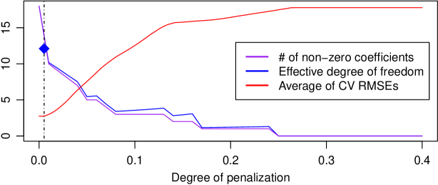
Figure 5: Effective degree of freedom with LAAD penalization

Note that not only the choice of tuning parameters, but we also might need to consider different attributes of covariates (for example, binary, ordinal, discrete, or continuous) when we do the variable selection with penalization. However, since the covariates used in our empirical analysis are all binary variables, we can claim that either direct use of $L_{1}$ penalty or its transformation is innocuous. For the variable selection on the covariates with diverse attributes, see Devriendt et al., (2018), which is reduced to an application of usual LASSO penalty in our case with only binary variables as covariates.

Once the parameters are estimated in each model, the corresponding incremental development factor $j^{th}$ lag for $n^{th}$ line of business can be also estimated as $\exp(\hat{\zeta}^{(n)}_{j})$, based on the formulation of lognormal cross-classified model. Table 6 summarizes the estimated results of incremental development factors for the calibrated models. One can see that the unconstrained model deviates from our expectations on the development pattern. For example, in the case of General Liability, incremental development factor of $7^{th}$ lag is less than that of $8^{th}$ lag. In the case of Other Casualty, it is also shown that incremental development factor of $9^{th}$ lag is less than 1, which is not intuitive as well. In contrast, it is observed that all constrained models and best subset selection model are able to perform the variable selection and impose smoothness on the sequences of development factors.

However, as mentioned in subsection 2.1, use of any penalization method induces bias on the non-zero coefficients while it is not desirable to have huge bias on the non-zero coefficients, due to the imposed shrinkage for smoothing the development factors. More specifically, it is likely that year-to-year development factors are relatively large at the earlier stage of the development. If we use LASSO, the coefficients of early development stage might be underestimated because the soft-thresholding affects all the coefficients regardless of how much a coefficient deviates from zero. This causes bias on the estimated coefficients, which induces less conservative reserve estimates. In Table 6, it is shown that both LAAD and LASSO regression have the same number of estimated non-zero coefficients but less shrinkage is applied on the coefficients from LAAD regression. Therefore, we think asymptotic unbiasedness of LAAD penalty supports achieving these two tasks simultaneously: smoothing the development factors and avoiding huge bias on the estimated non-zero coefficients.

Table 6: Summary of estimated incremental development factors

	General Liability						Other Casualty
	Unconstrained	Best	LASSO	SCAD	MCP	LAAD	Unconstrained	Best	LASSO	SCAD	MCP	LAAD
$\exp{(\zeta_{2})}$	2.2022	2.3527	2.3545	2.3067	2.2923	2.3006	1.2975	1.3861	1.4115	1.3590	1.3505	1.3657
$\exp{(\zeta_{3})}$	1.5681	1.5681	1.5253	1.5681	1.5681	1.5433	1.1052	1.1052	1.0948	1.1052	1.1052	1.0965
$\exp{(\zeta_{4})}$	1.3108	1.3108	1.2723	1.3108	1.3108	1.2875	1.0792	1.0000	1.0679	1.0508	1.0674	1.0706
$\exp{(\zeta_{5})}$	1.1723	1.1723	1.1349	1.1723	1.1723	1.1493	1.0352	1.0000	1.0231	1.0000	1.0000	1.0262
$\exp{(\zeta_{6})}$	1.1569	1.1569	1.1164	1.1569	1.1569	1.1321	1.0298	1.0000	1.0162	1.0000	1.0000	1.0200
$\exp{(\zeta_{7})}$	1.0465	1.0000	1.0053	1.0022	1.0030	1.0209	0.9959	1.0000	1.0000	1.0000	1.0000	1.0000
$\exp{(\zeta_{8})}$	1.0512	1.0000	1.0033	1.0000	1.0000	1.0215	1.0024	1.0000	1.0000	1.0000	1.0000	1.0000
$\exp{(\zeta_{9})}$	1.0106	1.0000	1.0000	1.0000	1.0000	1.0000	0.9929	1.0000	1.0000	1.0000	1.0000	1.0000
$\exp{(\zeta_{10})}$	1.0147	1.0000	1.0000	1.0000	1.0000	1.0000	0.9589	1.0000	1.0000	1.0000	1.0000	1.0000

4.3 Model validation

To validate the predictive models for loss development, calibrated using the training set (upper loss triangles) $\mathcal{D}_{1:10}$ defined in (6), we use cumulative (or incremental) payments of claims for calendar year 2012 as a validation set, obtained from ACE Limited 2012 Global Loss Triangles. Note that these data points can be described as $\mathcal{D}_{11}=\{Y{{}_{ij}^{(n)}}:2\leq i\leq 10\text{ and }j=12-i,n=1,2\}$ and they are displayed as semi-diagonals in blue color in the triangles of Tables 3 and 4.

Based on the estimated incremental development factor, one can predict cumulative (or incremental) payments of claims for the subsequent calendar year. For example, according to the model specification in (9), it is possible to predict the cumulative payment for $i^{th}$ accident year at $j+1^{th}$ lag as of $j^{th}$ lag as follows:

$$\hat{Y}^{(n)}_{i,j+1}=Y_{i,j}\times{\mathbb{E}}\left[Y^{(n)}_{i,j+1}/Y^{(n)}_{i,j}\right]=Y_{i,j}\times{\mathbb{E}}\left[\exp(C^{(n)}_{i,j})\right]=Y_{i,j}\times\exp\left(\zeta_{j+1}^{(n)}+{\frac{1}{2}\sigma^{2}}\right).$$

Table 7 provides the predicted values of incremental claims under each model as point estimates. According to the table, we can see that in case of Other Casualty line, LAAD model is the best for prediction of total unpaid claims for next calendar year. It is also shown that the Unconstrained model fails to perform the variable selection appropriately on the later development factors so that it severely underestimates incremental claims of older accidental years. In case of General Liability line, Best / SCAD / MCP models perform marginally well for the prediction of total unpaid claims, while LASSO model substantially underestimates the unpaid claims.

Table 7: Summary of predicted incremental paid claims

	General Liability							Other Casualty
	Unconstrained	Best	LASSO	SCAD	MCP	LAAD	Actual	Unconstrained	Best	LASSO	SCAD	MCP	LAAD	Actual
AY=2004	14,647	4,986	5,301	4,803	4,746	4,932	10,460	-11,930	2,751	2,925	2,650	2,619	2,722	1,702
AY=2005	12,610	5,250	5,582	5,058	4,998	5,194	18,236	275	2,944	3,130	2,836	2,803	2,912	4,655
AY=2006	57,778	7,520	11,266	7,244	7,159	28,505	42,420	4,514	3,386	3,600	3,262	3,224	3,350	1,098
AY=2007	42,162	5,964	10,479	7,449	8,013	22,093	49,790	1,575	3,213	3,417	3,096	3,059	3,179	6,641
AY=2008	175,372	175,194	132,625	174,848	174,740	148,629	62,450	16,338	3,335	10,599	3,213	3,175	12,000	24,195
AY=2009	128,676	128,555	102,272	128,319	128,246	112,112	116,112	29,856	5,329	21,723	5,134	5,073	23,477	23,449
AY=2010	145,081	144,995	127,759	144,827	144,775	134,362	152,345	35,583	3,142	31,120	23,789	30,540	31,980	11,790
AY=2011	173,204	173,136	160,477	173,003	172,962	165,626	220,413	56,300	56,220	51,295	56,065	56,017	51,845	55,776
AY=2012	165,965	186,556	186,954	180,158	178,152	179,383	203,434	139,542	179,970	191,861	167,408	163,468	170,580	165,383
Total	915,495	832,154	742,714	825,710	823,791	800,836	875,659	272,051	260,290	319,670	267,454	269,979	302,046	294,690

It is also possible to evaluate the performance of prediction based on usual validation measures such as root mean squared error (RMSE) and mean absolute error (MAE) defined as follows:

$$\text{RMSE }=:\sqrt{\frac{1}{9}\sum_{i=2}^{10}(\hat{Y}^{(n)}_{i,12-i}-Y^{(n)}_{i,12-i})^{2}},\quad\text{MAE }=:\frac{1}{9}\sum_{i=2}^{10}|\hat{Y}^{(n)}_{i,12-i}-Y^{(n)}_{i,12-i}|.$$

Table 8 shows us that LAAD model is the most preferred in terms of prediction performance measured by RMSE and MAE in both lines of business. One can see that LAAD model is the best in terms of out-of-sample validation except for the case of RMSE of General Liability line, in which LASSO model is the best followed by LAAD model.

Table 8: Summary of validation measures

	General Liability						Other Casualty
	Unconstrained	Best	LASSO	SCAD	MCP	LAAD	Unconstrained	Best	LASSO	SCAD	MCP	LAAD
RMSE	43381.92	45677.11	36949.02	45782.23	45827.07	37279.38	13246.63	12032.92	10915.02	10248.55	11335.33	8299.45
MAE	27803.04	32653.29	30366.00	33240.06	33413.07	27464.62	10101.76	8231.78	7903.88	6898.50	7642.07	5557.39

In actuarial practice, it is natural to consider possible ranges of reserve estimates in order to account for random deviation due to model, parameter, and stochastic errors. Despite the prevalent use of standard errors and $t$-test based on the asymptotic properties of maximum likelihood estimates, computation of standard errors in the penalization models has been controversial. There is generally no consensus or agreement on a statistically valid method to calculate standard errors for penalized regression (Kyung et al.,, 2010). For our purpose, we incorporate possible random deviation of predicted incremental claims using bootstrap methods as in Shi and Frees, (2011) and Gao, (2018), which can consider both parameter and stochastic errors simultaneously. From Table 9 and Figure 6, one can see that simulated unpaid claims under each model tend to be centered around the point estimates of total unpaid claims given in Table 7. All six models have intervals covering the actual unpaid claims. Details of simulation scheme with bootstrap is provided in Appendix C.

Table 9: Interval estimates of predicted incremental claims via bootstrap

	General Liability			Other Casualty
	Mean	95% L.I	95% U.I	Mean	95% L.I	95% U.I
Unconstrained	915,495	658,772	1,209,463	272,051	135,370	433,019
Best	742,714	574,713	1,029,077	319,670	174,127	382,608
LASSO	832,154	501,542	899,414	260,290	266,570	482,086
SCAD	825,710	622,338	1,069,123	267,454	170,353	408,123
MCP	823,791	605,001	1,064,936	269,979	163,782	409,046
LAAD	800,836	567,726	987,500	302,046	232,046	454,347
Actual	875,659			294,690

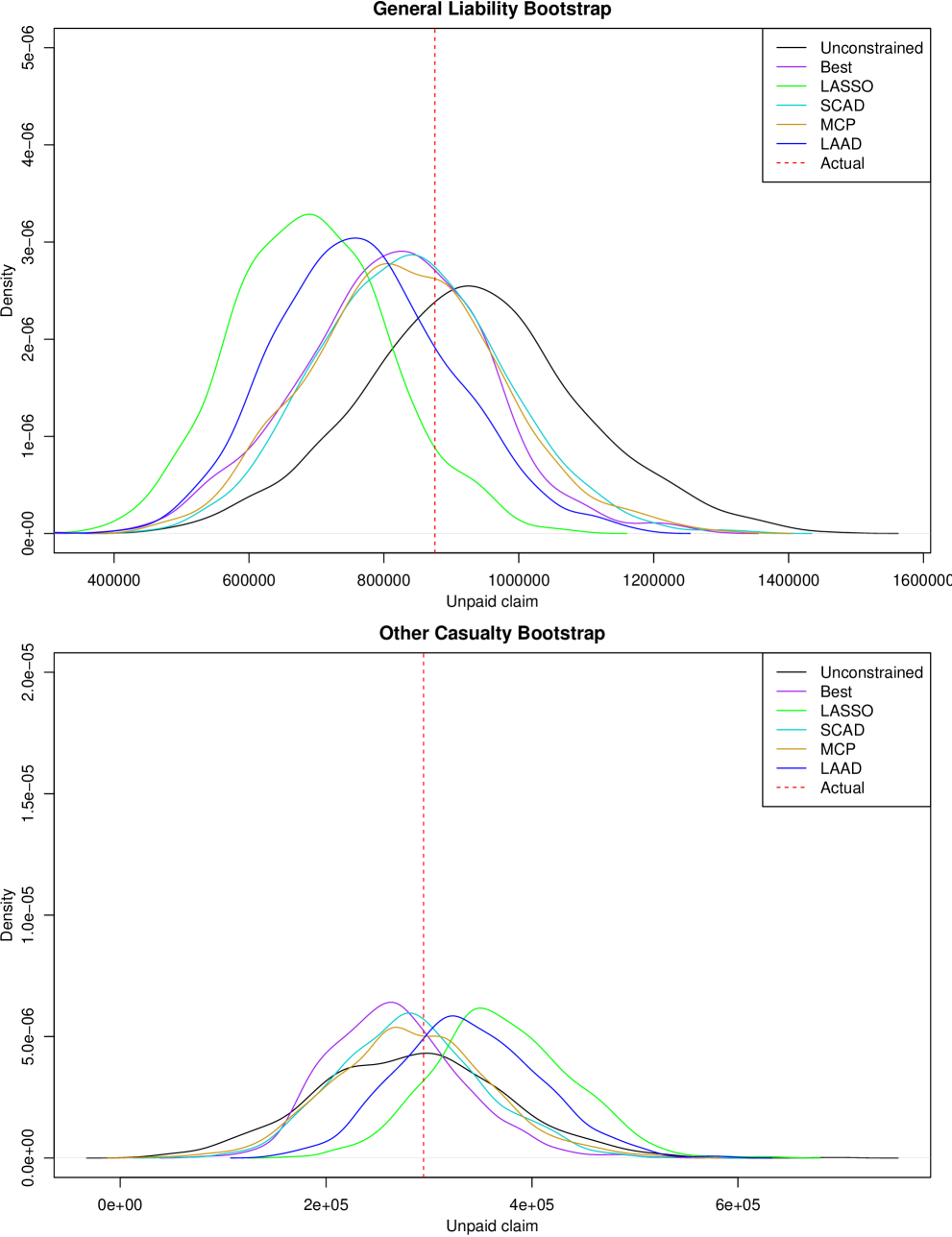
Figure 6: Predictive density of incremental reported losses for each model via Bootstrap

Although we focused on the possible application of non-convex penalization in aggregate reserving, we may not preclude use of LAAD penalization to other possible applications in actuarial science and insurance. For the interested readers, please see Appendix D for additional real data analysis, which examines a possible use of non-convex LAAD penalization in insurance ratemaking.

5 Concluding remarks

In this paper, we introduce use of LAAD penalty to obtain stable estimation of loss development factors. It is also shown that the proposed penalization method has some desirable properties such as the variable selection with reversion to the true regression coefficients, analytic solution for the univariate case, and an optimization algorithm for the multivariate case, which converges under modest condition within a coordinate descent algorithm. The novelty and performance of the proposed method are also shown using a simulation study. In this study, the use of LAAD regression outperforms other methods such as OLS and other non-convex penalization in terms of better prediction and the ability to capture the correct level of model sparsity. Furthermore, according to the results of the empirical application, the use of LAAD regression resulted in a reasonable loss development pattern with modest regularization and better prediction of unpaid claims for the subsequent calendar year. The results of the use of other non-convex regularization methods, however, are still within tolerance. For future research, one can extend the use of LAAD regression to more granular loss reserving models, which would naturally incorporate much more covariates.

Appendix A. Proof of Theorem 1

It is easy to see that $\hat{\theta}\times z\geq 0$ so we can start from the case that $z$ is not a negative number. Then we have the following:

$$\ell^{\prime}(\theta|r,z)=(\theta-z)+\frac{r}{1+\theta},\ \ell^{\prime\prime}(\theta|r,z)=1-\frac{r}{(1+\theta)^{2}},$$

$$\ell^{\prime}(\theta^{*})=0\Leftarrow\theta^{*}=\frac{z-1}{2}+\frac{\sqrt{(z-1)^{2}+4z-4r}}{2}$$

Note that if $z=r=1$, then $\ell^{\prime\prime}(\theta)=(\theta^{2}+2\theta)/(1+\theta)^{2}>0$ for $\theta>0$ and $\theta^{*}=0$. Thus, $\hat{\theta}=0$.

Case 1) $z\geq r$

Since $\hat{\theta}$ should be non-negative, we just need to consider $\theta^{*}=\frac{z-1}{2}+\frac{\sqrt{(z-1)^{2}+4z-4r}}{2}$. If $z\leq 1$, then

$$4(1+\theta^{*})^{2}\geq(z+1+|z-1|)^{2}=2^{2}>4r\ \Rightarrow\ \therefore\ l^{\prime\prime}(\theta^{*}|r,z)>0.$$

If $z>1$, then we have

$$4(1+\theta^{*})^{2}\geq(z+1+|z-1|)^{2}=4z^{2}>4z\geq 4r\ \Rightarrow\ \therefore\ l^{\prime\prime}(\theta^{*}|r,z)>0.$$

Thus, for both cases we have only one local minimum point $\theta^{*}$ for $l^{\prime}(\theta|r,z)$ and $\theta^{*}$ is indeed, a global minimum point so that $\hat{\theta}=\frac{z-1}{2}+\frac{\sqrt{(z-1)^{2}+4z-4r}}{2}$.

Case 2) $z<r,z<1$

In this case, $\theta^{*}<0$ so that $l^{\prime}(\theta|r,z)>0$ $\forall\theta\geq 0$. Therefore, $l(\theta|r,z)$ strictly increasing and $\hat{\theta}=0$.

Case 3) $r\geq(\frac{z+1}{2})^{2}$

In this case, $\theta^{*}\notin\mathbb{R}$. Moreover, $(\frac{z+1}{2})^{2}\geq z$, $l^{\prime}(0|r,z)=r-z\geq 0$ and $l^{\prime}(\theta|r,z)>0$ $\forall\theta>0$. Therefore, $\hat{\theta}=0$.

Case 4) $1\leq z<r<(\frac{z+1}{2})^{2}$

Here, let $\theta^{*}=\frac{z-1}{2}+\frac{\sqrt{(z-1)^{2}+4z-4r}}{2}$ and $\theta^{{}^{\prime}}=\frac{z-1}{2}-\frac{\sqrt{(z-1)^{2}+4z-4r}}{2}$. Now, let us show that $\theta^{*}$ is the local minimum of $\ell(\theta|r,z)$ - which only requires to show that $\ell^{\prime\prime}(\theta^{*}|r,z)>0$. Again, it suffices to show that $4(1+\theta^{*})^{2}>4r$ as follows:

$$4(1+\theta^{*})^{2}=(z+1+\sqrt{(z+1)^{2}-4r})^{2}>(z+1)^{2}+(z+1)^{2}-4r>4r\ \Rightarrow\ \therefore\ \ell^{\prime\prime}(\theta^{*}|r,z)>0.$$

Therefore, $\theta^{*}$ is a local minimum of $\ell(\theta|r,z)$ and $\hat{\theta}$ would be either $\theta^{*}$ or $0$. So in this case, we have to compute $\Delta(z|r)=\ell(\theta^{*}|r,z)-\ell(0|r,z)$ and

$$\hat{\theta}=\begin{cases}\theta^{*}\ ,\quad\text{if }\Delta(z|r)<0,\\ 0\quad,\quad\text{if }\Delta(z|r)>0\end{cases}$$

Note that for fixed $r$,

$$\Delta(z|r) =\frac{1}{2}(\theta^{*})^{2}-\theta^{*}z+r\log(1+\theta^{*}),$$

$$\Delta^{\prime}(z|r) =(\theta^{*}-z+\frac{r}{1+\theta^{*}})\frac{\partial\theta^{*}}{\partial z}-\theta^{*}$$

$$=-\theta^{*}\quad(\because\ l(\theta^{*}|r,z)=\theta^{*}-z+\frac{r}{1+\theta^{*}}=0)$$

Thus, $\Delta(z|r)$ is strictly decreasing with respect to $z$ and

$$\Delta(z|r) =\frac{1}{2}(\theta^{*})^{2}-\theta^{*}z+r\log(1+\theta^{*})$$

$$=\frac{1}{2}\left(\frac{z-1}{2}+\frac{\sqrt{(z-1)^{2}+4z-4r}}{2}\right)^{2}-\left(\frac{z-1}{2}\frac{\sqrt{(z-1)^{2}+4z-4r}}{2}\right)z$$

$$\quad+r\log\left(\frac{z+1}{2}+\frac{\sqrt{(z-1)^{2}+4z-4r}}{2}\right)=0$$

has unique solution because $\Delta(z|r)<0\Leftrightarrow\hat{\theta}=\theta^{*}$ if $z=r$ and $\Delta(z|r)>0\Leftrightarrow\hat{\theta}=0$ if $z=2\sqrt{r}-1$. Hence

$$\hat{\theta}=\left(\frac{z-1}{2}+\frac{\sqrt{(z-1)^{2}+4z-4r}}{2}\right)(\mathbbm{1}_{\{z\geq z^{*}(r)\}}).$$

where $z^{*}(r)$ is the unique solution of $\Delta(z|r)=0$ for given $r$. See Figure 7.

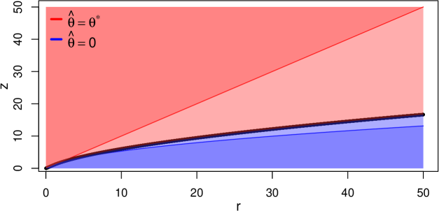
Figure 7: Distribution of optimizer along with r and z

Once we get a result for $z\geq 0$, we can use the same approach to $l(\theta|r,-z)$ when $z<0$.

Appendix B. Proof of Lemma 1

Suppose $\beta_{j}$ is fixed as $w_{j}$ for all $j=1,\ldots,k-1,k+1,\ldots,p$. Then we can observe that

$$\ell_{k}(\theta) =\frac{1}{2}\bigg{|}\bigg{|}(y-\sum_{j\neq k}X_{j}w_{j})-X_{k}\theta\bigg{|}\bigg{|}^{2}+r\log(1+|\theta|)+r\sum_{j\neq k}\log(1+|w_{j}|)$$

$$=\frac{1}{2}||t_{k}-X_{k}\theta||^{2}+r\log(1+|\theta|)+r\sum_{j\neq k}\log(1+|w_{j}|)$$

$$=\frac{1}{2}(\theta^{\prime}X^{\prime}_{k}X_{k}\theta-2\theta X_{k}^{\prime}t_{k}+t_{k}^{\prime}t_{k})+r\log(1+|\theta|)+r\sum_{j\neq k}\log(1+|w_{j}|)$$

$$=\frac{1}{2}(\theta-z_{k})^{2}+r\log(1+|\theta|)+C_{k}$$

where $C_{k}=\frac{1}{2}(t_{k}^{\prime}t_{k}-t_{k}^{\prime}X_{k}X_{k}^{\prime}t_{k})+r\sum_{j\neq k}\log(1+|w_{j}|)$ and $z_{k}=X_{k}^{\prime}t_{k}$.

As usual, we can start from the case that $z_{k}\geq 0$. First, one can easily check that $\ell_{k}(\theta)$ is a decreasing function of $\theta$ where $\theta\leq 0$ and $z_{k}\geq 0$. When $\theta>0$, according to the arguments in the proof of Theorem 1, $l_{k}(\theta)$ is strictly decreasing when $\theta\in(0,\theta^{*}]$ and strictly increasing when $\theta\in[\theta^{*},\infty)$ if $r$ and $z_{k}$ belong to Case 1, Case 2, and Case 3. Note that if $r\leq 1$, then we may exclude Case 4. Therefore, $l_{k}(\theta)$ is hemivariate and quasi-convex if $z_{k}\geq 0$ and also if $z_{k}<0$ because of the symmetry of penalty term.

Appendix C. Bootstrap for predictive distribution of unpaid loss

• Simulate $\{\hat{c}^{(n)}_{ij[s]}|\,i=1,\ldots,I,\,j=1,\ldots J-I+1,\,n=1,2\}$ where $\log\hat{c}^{(n)}_{ij[s]}\sim\mathcal{N}(\hat{\eta}_{ij}^{(n)},\hat{\sigma}^{2})$.

• Using the simulated values of $\hat{c}^{(n)}_{ij[s]}$ in step (1), estimate bootstrap replication of the parameters $\{(\hat{\eta}_{ij[s]}^{(n)},\hat{\sigma}_{[s]}^{2})|\,i=1,\ldots,I,\,j=1,\ldots J-I+1,\,n=1,2\}$.

• Based on $(\hat{\eta}_{ij[s]}^{(n)},\hat{\sigma}_{[s]}^{2})$, predict the unpaid loss ${L}^{(n)}$ for the next year which is given as follows:

  $$\hat{L}^{(n)}_{[s]}=\sum_{i=2}^{10}\left(\exp{(\hat{\eta}_{i,12-i[s]}^{(n)}+\hat{\sigma}_{[s]}^{2}/2)}-1\right)y^{(n)}_{i,11-i}$$

  Note that the values of $y^{(n)}_{i,11-i}$ for $i=2,\ldots,10$ and $n=1,2$ are already known in advance from the training set.

• Repeat steps (1), (2), and (3) for $s=1,\ldots,S$ to obtain the predictive distribution and standard error of ${L}^{(n)}$.

Appendix D. Application of LAAD penalty in insurance ratemaking

To illustrate possible use of LAAD penalized regression for insurance ratemaking, we used the LGPIF (Wisconsin Local Government Property Insurance Fund) data, which consists of policy characteristics and claims information on multiple lines of business. Each observation is a local government unit such as city, town, village, or county. For simplicity, among the multiple types of claims, we extracted the information from IM (inland marine) line of business only. We used 235 observations with positive claim amounts with corresponding policy characteristics summarized in Table 10.

Table 10: Observable policy characteristics used as covariates

Categorical	Description		Proportions
variables
TypeCity	Indicator for city entity:	Y=1	24.26 %
TypeCounty	Indicator for county entity:	Y=1	42.55 %
TypeMisc	Indicator for miscellaneous entity:	Y=1	0.43 %
TypeSchool	Indicator for school entity:	Y=1	5.96 %
TypeTown	Indicator for town entity:	Y=1	8.08 %
TypeVillage	Indicator for village entity:	Y=1	18.72 %
NoClaimCreditIM	No IM claim in three consecutive prior years:	Y=1	37.02 %
Continuous		Minimum	Mean	Maximum
variables
CoverageIM	Log coverage amount of IM claim in mm	0.02	5.05	46.75
lnDeductIM	Log deductible amount for IM claim	6.215	6.751	8.517

Since the original dataset is quite rich for data analysis, one can consider several different aspects of ratemaking, such as the heavy-tail behavior of claims, possible dependence between frequency and severity, and serial dependence among the claims of the same policyholder when observed over time. We do not consider the aformentioned topics to avoid distraction, but we refer the interested readers to Frees et al., (2016), Lee and Shi, (2019), and Jeong, (2020).

The observed total positive claim amount, $S_{i}$, can be described as follows:

$$\ln S_{i}\sim{\mathcal{N}}\left(\mu_{i},\sigma^{2}\right)\ \text{ and }\mu_{i}=\mathbf{x}_{i}\beta,$$

and six different competing models were examined for calibration.

• Unconstrained model: a model which minimizes the following objective function:

  $$\sum_{i=1}^{m}\left(\ln S_{i}-\mathbf{x}_{i}\beta\right)^{2},$$

• Best subset model: a model which minimizes Bayesian information criterion (BIC) based on the estimated parameter values.

• LASSO / SCAD / MCP / LAAD constrained models: models which minimize the following objective functions with $p_{\lambda}(\cdot)$ as defined in (4):

  $$\sum_{i=1}^{m}\left(\ln S_{i}-\mathbf{x}_{i}\beta\right)^{2}+\left[\sum_{k=1}^{p}p_{\lambda}\left(\beta_{k}\right)\right],$$

As usual, note that for all constrained models, we do not impose penalty constraint on $\beta_{0}$, the intercept coefficient.

Table 11 summarizes the estimated coefficients of ratemaking factors. One can see that originally we have six types of location variables but we end up with three types of location variables (City, County, and Others) after variable selection is performed using regularization methods. One can also immediately deduce an intuitive explanation to these results. For example, City and County are some of the largest government entities. Coincidentally, the estimated coefficients happen to be identical for Best, SCAD, and MCP models.

Table 11: Summary of estimated ratemaking factors

	Unconstrained	Best	LASSO	SCAD	MCP	LAAD
TypeCity	1.1342	1.0352	0.6890	1.0352	1.0352	0.5655
TypeCounty	0.7239	0.6125	0.3243	0.6125	0.6125	0.1851
TypeMisc	-0.5596	-	-	-	-	-
TypeSchool	0.3957	-	-	-	-	-
TypeTown	0.0397	-	-	-	-	-
CoverageIM	0.0497	0.0483	0.0460	0.0483	0.0483	0.0486
lnDeductIM	-0.0246	-	-	-	-	-
NoClaimCreditIM	0.0839	-	-	-	-	-

Table 12 shows that LAAD regression is the best performing model in terms of out-of-sample validation measures, and followed by LASSO regression. We conclude that regularization methods can also be applied to insurance ratemaking problems so that one can effectively reduce the dimension of ratemaking factors that can be used and still have better prediction performance.

Table 12: Summary of validation measures

	Unconstrained	Best	LASSO	SCAD	MCP	LAAD
RMSE	22039.11	23029.08	16895.38	23029.08	23029.08	15498.43
MAE	19330.80	20393.52	15504.69	20393.52	20393.52	14279.56

References

- Armagan et al., (2013) Armagan, A., Dunson, D. B., and Lee, J. (2013). Generalized double Pareto shrinkage. Statistica Sinica, 23(1):119.
- Chan et al., (1982) Chan, F., Chan, L., and Mead, E. (1982). Properties and modifications of Whittaker-Henderson graduation. Scandinavian Actuarial Journal, 1982:57–61.
- Devriendt et al., (2018) Devriendt, S., Antonio, K., Reynkens, T., and Verbelen, R. (2018). Sparse regression with multi-type regularized feature modeling. arXiv preprint arXiv:1810.03136.
- Efron, (1986) Efron, B. (1986). How biased is the apparent error rate of a prediction rule? Journal of the American Statistical Association, 81(394):461–470.
- Fan and Li, (2001) Fan, J. and Li, R. (2001). Variable selection via nonconcave penalized likelihood and its oracle properties. Journal of the American Statistical Association, 96(456):1348–1360.
- Frees et al., (2016) Frees, E. W., Lee, G., and Yang, L. (2016). Multivariate frequency-severity regression models in insurance. Risks, 4(1):4.
- Friedman et al., (2009) Friedman, J., Hastie, T., and Tibshirani, R. (2009). glmnet: Lasso and elastic-net regularized generalized linear models. R package version 4.0-2.
- Gao, (2018) Gao, G. (2018). Bayesian Claims Reserving Methods in Non-life Insurance with Stan. Springer.
- Hastie et al., (2009) Hastie, T., Tibshirani, R., and Friedman, J. (2009). The elements of statistical learning: data mining, inference, and prediction. Springer Science & Business Media.
- Hastie et al., (2015) Hastie, T., Tibshirani, R., and Wainwright, M. (2015). Statistical learning with sparsity: the lasso and generalizations. CRC press.
- Hoerl and Kennard, (1970) Hoerl, A. E. and Kennard, R. W. (1970). Ridge regression: Biased estimation for nonorthogonal problems. Technometrics, 12(1):55–67.
- James et al., (2013) James, G., Witten, D., Hastie, T., and Tibshirani, R. (2013). An Introduction to Statistical Learning. Springer.
- Jeong, (2020) Jeong, H. (2020). Testing for random effects in compound risk models via Bregman divergence. ASTIN Bulletin: The Journal of the IAA, 50(3):777–798.
- Jeong and Dey, (2020) Jeong, H. and Dey, D. K. (2020). Application of vine copula for multi-line insurance reserving. Risks, 8(4):111.
- Knight and Fu, (2000) Knight, K. and Fu, W. (2000). Asymptotics for lasso-type estimators. The Annals of Statistics, 28(5):1356–1378.
- Kyung et al., (2010) Kyung, M., Gill, J., Ghosh, M., and Casella, G. (2010). Penalized regression, standard errors, and Bayesian lassos. Bayesian Analysis, 5(2):369–411.
- Lee et al., (2010) Lee, A., Caron, F., Doucet, A., and Holmes, C. (2010). A hierarchical Bayesian framework for constructing sparsity-inducing priors. arXiv preprint arXiv:1009.1914.
- Lee and Shi, (2019) Lee, G. Y. and Shi, P. (2019). A dependent frequency–severity approach to modeling longitudinal insurance claims. Insurance: Mathematics and Economics, 87:115–129.
- Lumley, (2013) Lumley, T. (2013). R package ‘leaps’. R package version 3.1.
- Luo and Tseng, (1992) Luo, Z.-Q. and Tseng, P. (1992). On the convergence of the coordinate descent method for convex differentiable minimization. Journal of Optimization Theory and Applications, 72(1):7–35.
- Mack, (1993) Mack, T. (1993). Distribution-free calculation of the standard error of chain ladder reserve estimates. ASTIN Bulletin: The Journal of the IAA, 23(2):213–225.
- Mack, (1999) Mack, T. (1999). The standard error of chain ladder reserve estimates: Recursive calculation and inclusion of a tail factor. ASTIN Bulletin: The Journal of the IAA, 29(2):361–366.
- Mazumder et al., (2011) Mazumder, R., Friedman, J. H., and Hastie, T. (2011). Sparsenet: Coordinate descent with nonconvex penalties. Journal of the American Statistical Association, 106(495):1125–1138.
- McGuire et al., (2018) McGuire, G., Taylor, G., and Miller, H. (2018). Self-assembling insurance claim models using regularized regression and machine learning. Available at SSRN 3241906.
- Nawar, (2016) Nawar, S. M. (2016). Machine learning techniques for detecting hierarchical interactions in insurance claims models. Master’s thesis, Concordia University.
- Park and Casella, (2008) Park, T. and Casella, G. (2008). The Bayesian LASSO. Journal of the American Statistical Association, 103(482):681–686.
- Renshaw, (1989) Renshaw, A. E. (1989). Chain ladder and interactive modelling.(claims reserving and glim). Journal of the Institute of Actuaries, 116(3):559–587.
- Shi et al., (2012) Shi, P., Basu, S., and Meyers, G. G. (2012). A bayesian log-normal model for multivariate loss reserving. North American Actuarial Journal, 16(1):29–51.
- Shi and Frees, (2011) Shi, P. and Frees, E. W. (2011). Dependent loss reserving using copulas. ASTIN Bulletin: The Journal of the IAA, 41(2):449–486.
- Stein, (1981) Stein, C. M. (1981). Estimation of the mean of a multivariate normal distribution. The Annals of Statistics, 9(6):1135–1151.
- Taylor and McGuire, (2016) Taylor, G. and McGuire, G. (2016). Stochastic loss reserving using generalized linear models. Casualty Actuarial Society.
- Tibshirani, (1996) Tibshirani, R. (1996). Regression shrinkage and selection via the LASSO. Journal of the Royal Statistical Society. Series B (Methodological), 58(1):267–288.
- Tseng, (2001) Tseng, P. (2001). Convergence of a block coordinate descent method for nondifferentiable minimization. Journal of Optimization Theory and Applications, 109(3):475–494.
- Wang et al., (2019) Wang, S., Zhang, H., Chai, H., and Liang, Y. (2019). A novel log penalty in a path seeking scheme for biomarker selection. Technology and Health Care, 27(S1):85–93.
- Williams et al., (2015) Williams, B., Hansen, G., Baraban, A., and Santoni, A. (2015). A practical approach to variable selection—a comparison of various techniques. In Casualty Actuarial Society E-Forum, pages 4–40.
- Yin and Lin, (2016) Yin, C. and Lin, X. S. (2016). Efficient estimation of erlang mixtures using iscad penalty with insurance application. ASTIN Bulletin: The Journal of the IAA, 46(3):779–799.
- Zhang, (2010) Zhang, C.-H. (2010). Nearly unbiased variable selection under minimax concave penalty. The Annals of Statistics, 38(2):894–942.
- Zhang and Melnik, (2009) Zhang, C.-H. and Melnik, O. (2009). plus: Penalized linear unbiased selection. R package version 1.0.
- Zou et al., (2007) Zou, H., Hastie, T., and Tibshirani, R. (2007). On the “degrees of freedom” of the lasso. The Annals of Statistics, 35(5):2173–2192.