STT-CBS: A Conflict-Based Search Algorithm for Multi-Agent Path Finding with Stochastic Travel Times

Abstract

We present an algorithm for finding optimal paths for multiple stochastic agents in a graph to reach their destinations with a user-specified maximum pairwise collision probability. Our algorithm, called STT-CBS, uses Conflict-Based Search (CBS) with a stochastic travel time (STT) model for the agents. We model robot travel time along each edge of the graph by independent gamma-distributed random variables, and propose probabilistic collision identification and constraint creation methods to robustly handle travel time uncertainty. We show that under reasonable assumptions our algorithm is optimal in terms of expected sum of travel times, while ensuring an upper bound on each pairwise conflict probability. Simulations and hardware experiments show that STT-CBS is able to significantly decrease conflict probability over CBS, while remaining within the same complexity class.

1 Introduction

We are interested in routing a team of robots from an initial configuration to a target configuration through collision-free trajectories, represented as paths through a graph. Relevant applications include real-time vehicle routing [15], warehouse management [24], and unmanned aerial vehicle (UAV) coordination [7]. Typically in such applications, routes are planned offline for the whole team assuming known, deterministic nominal travel times for robots to traverse each node and edge in the graph. The planned paths are then executed by the robots through lower-level path following controllers. Unfortunately, real robots are stochastic. Hence the actual travel times for robots quickly depart from the nominal expected times in the plan, leading to potential unplanned robot-robot conflicts. If robots collide with one another, or need to take unplanned-for maneuvers to avoid collisions, this leads to further delays. This causes a cascading effect, making their travel times vary more widely from what was expected during planning, and leading to more potential downstream robot-robot conflicts. The consequent lack of predictability makes optimal planning on long time horizons challenging. To address this problem, we propose Stochastic Travel Time Conflict Based Search (STT-CBS), a planning algorithm that inherently plans for stochasticity in robots’ node and edge traversal times. STT-CBS minimizes robots’ expected travel time subject to a pairwise conflict probability among the robots.

We build upon the common Multi-Agent Path Finding (MAPF) problem formulation, wherein agents are allowed to move along the edges of a graph from their initial locations to prescribed destinations. Recently, optimal MAPF planners have shown their effectiveness empirically on a variety of problems [17, 5, 11], most of which assume the robots travel along edges in the graph with fixed, deterministic travel times. In contrast, in this work we focus on accounting for stochasticity in the robots’ travel times. This is important, as real robots (e.g., in a factory, or a warehouse) may not traverse an edge at exactly the intended rate. Real robots have to contend with wheel-slip, course-correction and collision avoidance actions, battery voltage fluctuations, and many other effects that randomly influence the time it takes them to traverse nodes and edges in the graph. If one ignores these random effects, the resulting trajectories may lead to collisions, and may yield significantly suboptimal total travel times in practice.

Our proposed algorithm, STT-CBS, is a MAPF planning algorithm that seeks to minimize the expected sum of travel times of the robots subject to a bound on the probability of collision for any pair of robots. By accounting for uncertainty in travel time due to environmental disturbances, STT-CBS improves the consistency and reliability in the actual execution of the robots’ planned paths. We model the time that each robot waits at a node of the graph as a gamma-distributed random variable. This model of randomness captures the sequential summing of uncertain effects along a trajectory as a robot passes through multiple nodes in the graph. We only ascribe random delays to the nodes in our model. Conceptually, we lump the delay due to edge traversal and node traversal into one random effect at the nodes only. We suppose it is more important to model random delays at the nodes, since they act as “intersections” in the road map, and hence are likely to be key choke points where robot-robot conflicts might occur. One can also ascribe separate random delays to the traversal of edges, but with an increased computational burden in the algorithm.

We show that if a solution exists, our algorithm will return the solution that minimizes expected total travel time subject to the probabilistic collision constraint. We compare STT-CBS against a baseline algorithm on a set of simulation experiments, showing that our algorithm can better prevent collisions under this stochastic travel time model. We also demonstrate our algorithm in hardware experiments, routing three ground robots from initial locations, through a graph, to goal locations in a lab environment, while accounting for the real-world stochasticity in their travel times.

2 Background and Related Work

In the discrete-time MAPF formulation, edges can be traversed in unit time, and each robot is assigned to a specific goal. The unit travel time is sometimes called the “pebble motion” problem [9], and each agent having an assigned goal is called the “labeled” case. The solution to a discrete-time MAPF problem is a joint assignment of trajectories such that no two agents occupy the same vertex or traverse the same edge at the same time (i.e., trajectories are free of conflict). This model is the basis of many graph-based multi-agent path finding algorithms [17, 22, 25]. However, robots often do not satisfy the strict assumptions of the pebble motion model. Recent work in MAPF has focued on more realistic robot models, such as continuous-time edge traversal [19] and probabilistic integer delays at nodes [2, 22]. Our algorithm, STT-CBS, is based on a more general model, where travel time for the robots is modeled as a continuous gamma-distributed random variable. One may choose to optimize a variety of different objective functions for MAPF problems, however the most common choices are to minimize total travel time (the sum of the lengths of all trajectories) [17, 25], or to minimize makespan (the travel time of the longest robot trajectory) [4]. In keeping with most of the literature, we choose to minimize total travel time, although our algorithm could be adapted to minimize makespan or other objectives.

Finding an optimal solution to the labeled discrete-time MAPF problem is NP-hard [26]. Optimal and complete MAPF solution methods (those that are guaranteed to find an optimal solution if it exists) can be broadly grouped into three categories: In (i) coupled approaches, the search for an optimal feasible solution is performed directly in the joint action space of the agents. (ii) Decoupled approaches operate by computing paths on an individual (per-agent) basis, and then resolving pairwise conflicts repeatedly by re-planning. This is the basis of Conflict-Based Search [17] and its variants [17], as well as the algorithm we propose in this paper, STT-CBS. There are also (iii) semi-coupled approaches, which group agents into teams or “meta-agents”, and then apply a de-coupled approach between the joint plans associated with each team. A representative example of a semi-coupled approach is Operator Decomposition and Independence Detection (OD+ID) [18].

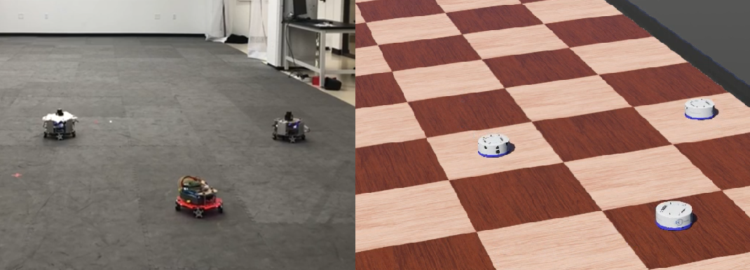
Figure 1: Our algorithm plans collision-free paths in a graph for robots that travel with stochastic travel times through a path in a graph. We evaluated the algorithm in hardware and simulation experiments with robots to verify the robustness of our approach to real-world stochastic delays.

The “pebble-motion” MAPF formulation abstracts away robot dynamics and does not account for uncertainty. In trying to execute paths specified by a MAPF planner, actuator dynamics and other disturbances will inevitably introduce errors that violate the assumptions of constant-velocity and unit-time edge traversal. This can be problematic when nominally “conflict-free” trajectories are not conflict-free during actual execution. One way to address this modeling error is to ignore it during planning, and then to incorporate closed-loop control for stabilizing robots to the commanded trajectories [12]. While this approach is simple and practical, it relies on important spacing around agents in order to avoid accumulating delays and deadlocks. It provides no means to predict or assess conflict probabilities and associated delays that may occur due to low-level controllers taking collision avoidance maneuvers. In automated warehouse and manufacturing applications, space efficiency, time efficiency, and predictability are essential [1]. To this end, we propose a solution that is able to perform more consistently in a cluttered environment, while allowing for a user to specify maximum pairwise conflict probability between robots.

Our algorithm builds upon Conflict-Based Search (CBS) [17], a state-of-the-art algorithm to solve the optimal MAPF problem. Many heuristics [6, 10] have been developed to accelerate CBS. It has also been merged with different planning methods [13] and extended to more complex agent geometries [11] and graphs that allow for non-unit edge traversal times [19]. None of these approaches are robust to conflicts that might occur due to delay in the actual execution of the robots’ paths. Stochastic travel times are important, since what may start as a small delay by one robot may snowball into a traffic jam that significantly delays all robots. Few MAPF approaches reason about robots’ execution uncertainty during the planning phase. [16] propose an algorithm to compute optimal conflict-free paths in worst-case scenarios under bounded travel times. While this model is more general than the traditional pebble-motion model, it fails to account for the probability of conflicts occurring. Thus, solutions where a highly unlikely travel time combination within the specified bounds results in a conflict are discarded, which makes the choice of conservative upper bounds particularly costly. Another algorithm that does reason about uncertain travel times is $k$-robust CBS, which seeks solutions that remain collision free considering that each agent may be delayed for up to $k$ time steps [3]. A downside of this model is that it fails to consider the sequential summing of delay as agents advance, which is key to capturing the snowballing effect of a traffic jam among the robots. In order to take this summing into account, Atzmon et al. have extended $k$-robust CBS to $p$-robust CBS [2]. The pR-CBS algorithm searches for solutions minimizing total travel time such that the probability of at least one conflict occurring during path execution is smaller than a threshold $p$. In this model, agents have a fixed probability of being delayed at their current node for one time step. This approach iterates over all possible solutions sorted by increasing cost until one is found that is feasible and has an overall conflict probability that is smaller than $p$. Alternatively, the UM^⋆ algorithm [22] also takes sequential summing of delay into account. In this approach, progress is modeled as a Markov Decision Process. This algorithm fits in the framework of M^⋆ [21], and provides an optimal planning solution for the MAPF problem within the pebble motion model. While the UM^⋆ algorithm is incomplete, it is empirically effective to compute optimal solutions for a large category of problems. Approximate Minimization in Expectation [14], based on the same model, computes solutions that approximately minimize expected makespan. One advantage of this method compared to the previous is that it takes into account the possibility that agents may collide with each other during path execution.

Our proposed algorithm, STT-CBS, similarly plans under stochastic travel times. However, it does not require the unrealistic assumptions within the pebble-motion model. Specifically, our model allows for the robots to have different travel speeds, accommodates non-unit time traversal of edges and nodes, and allows for gamma-distributed stochastic delays at nodes, where different nodes can have different parameters for their gamma distributions. Allowing for different robot speeds can better reflect the nominal time that robots take to navigate when accounting for surrounding obstacles, and the gamma-distributed delay at different nodes may be adjusted to differentiate areas where sources of uncertainty, such as obstacles or people, are more or less present.

3 Approach

Here we formalize the stochastic travel time MAPF problem under consideration. As in the deterministic travel time formulation, each agent must move from its initial location to a prescribed final location without collision with other agents. The task is to find a solution that minimizes the expected total travel time subject to the constraint that the likelihood of collision for each pair of agents at any place in the graph is below some threshold $\epsilon\in[0,1]$. While we present the algorithm as an offline planner for clarity, in practice one could re-solve for the agents’ trajectories periodically during execution in a receding horizon fashion, in order to incorporate real time knowledge of the agents’ locations and delays up to that point.

3.1 Problem Setup

We consider a team of robots simultaneously traversing paths on a graph $\mathcal{G}=(\mathcal{V},\mathcal{E})$, where $\mathcal{V}=\{1,\ldots,N\}$ is a set of nodes of the graph and $\mathcal{E}=\{\ldots,(i,j),\ldots\}$ is a set of edges. We denote the discrete path taken by robot $i$ through the graph by the tuple $P_{i}=(p_{i}(0),p_{i}(1),\ldots,p_{i}(K_{i}))$, with discrete path length $K_{i}$, and we require that all neighboring nodes in this tuple are linked by edges in the graph, $e_{i}(k)=(p_{i}(k-1),p_{i}(k))\in\mathcal{E}$. Physically, the nodes in the graph represent points in the environment, and the edges represent physical paths between those points, which require some finite time for the robot to traverse. Each edge in the graph has a travel time $t_{e}$, and if robot $i$ traverses edge $e$ at time $k$, we say $t_{e_{i}}(k)=t_{e}$. We model the time that a robot $i$ waits at the $k$th node in its path as a real-valued time duration $\tau_{i}(k)$. The robot may need to wait at a node to avoid a collision, while another robot passes through neighboring edges or vertices. We model this waiting time with a gamma distributed random variable. One can also ascribe random travel times to the robots’ edge traversals, although we do not do so in this work. Thus, the history of time durations for the path of robot $i$ is given by both the sequence of deterministic edge traversal times $T_{ei}=(t_{e_{i}}(1),\ldots,t_{e_{i}}(K_{i}))$ and stochastic vertex traversal times $T_{vi}=(\tau_{i}(0),\ldots,\tau_{i}(K_{i}))$. Together, $P_{i}$, $T_{ei}$ and $T_{vi}$ define the trajectory of robot $i$.

3.2 Uncertainty Model

In warehouse or factory-floor settings, robots have low-level controllers that control them to track a desired path. However, disturbances are likely to occur as delays along the prescribed path due to wheel slip, feedback corrections from the low-level controller, unexpected minor obstacles, and other sources of stochastic delay. Our particular choice of travel time model is motivated by this phenomenon of stochastic accumulating delay for factory or warehouse robots.

We model delay at each node of an agent’s trajectory as a random variable following a gamma distribution. More precisely, we consider that each time a node $v$ is traversed by $\text{Robot }{i}$, then the robot is delayed, and the delay $\tau_{v,i}$ is a random variable described by $\tau_{v,i}\sim\text{Gamma}(n_{v},\lambda)$. The more nodes and edges traversed by each agent, the larger its expected delay and uncertainty in its position along its route in the graph.

3.3 Computing Conflict Probability

In this section, we express the probability of a conflict between two agents as a function of our model parameters. Figure 2 illustrates how a conflict can happen in this stochastic model.

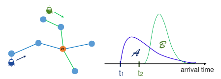
Figure 2: Conflict identification at a node $n$. Blue and green robots are scheduled to arrive at node $n$ at different times, $t_{1}$ and $t_{2}$. Distributions $\mathcal{A}$ and $\mathcal{B}$ illustrate the probability density of the blue and green robot’s arrival time respectively. Although their arrival times are different, uncertainty over travel time may cause them occupy node $n$ at overlapping time intervals, causing a conflict. If the green robot arrives at $n$ before the blue robot departs from $n$, and if the blue robot arrives before the green robot departs, then the robots will conflict with each other.

3.3.1 Cumulative delay

Let $\text{Robot }{i}$ be assigned a path $P_{i}$. At the start of its route, it is not delayed. As it progresses along its route, it is delayed at each node $v$ by some value $\tau_{i}(k)$ in addition to its planned travel time, with $\tau_{i}(k)\sim\text{Gamma}(n_{v},\lambda)$. We note the total delay accumulated by $\text{Robot }{i}$ when it arrives to the $k$th node on its path as $\Delta_{i}(k)=\sum_{0}^{k}\tau_{i}(k)$.

For simplicity, we use a rate parameter $\lambda$ in the Gamma distribution that is identical across all the nodes in our graph. To account for different travel time distributions, we can vary the shape parameter $n_{v}$. Conveniently, the sum of $N$ independent gamma-distributed random variables with shape parameters $n_{v}$ and identical rate parameter $\lambda$ is a gamma-distributed random variable with shape parameter $\sum_{v=1}^{N}n_{v}$ and rate parameter $\lambda$. Thus we can write the delay accumulated by $\text{Robot }{i}$ along its trajectory up to time $k$ as

$$\Delta_{i}(k)\sim\text{Gamma}\left(\sum_{j=0}^{k}n_{p_{i}(j)},\lambda\right).$$ (1)

Using this stochastic delay, we can express the probability of a conflict between two robots, $\text{Robot }{1}$ and $\text{Robot }{2}$, at a particular node or edge. Dropping the index $k$ and defining $n_{1}=\sum_{j=0}^{k}n_{p_{1}(j)}$ and $n_{2}=\sum_{j=0}^{k}n_{p_{2}(j)}$ for notational simplicity, we will denote the cumulative delays for each agent $\Delta_{1}\sim\text{Gamma}(n_{1},\lambda)$ and $\Delta_{2}\sim\text{Gamma}(n_{2},\lambda)$.

3.3.2 Node Conflicts

The probability of a conflict between $\text{Robot }{1}$ and $\text{Robot }{2}$ at node $v$ is computed as follows. Let $t_{1}$ and $t_{2}$ denote the nominal times (as computed without any stochastic delays) at which $\text{Robot }{1}$ and $\text{Robot }{2}$ are scheduled to arrive at $v$, respectively. The actual arrival times depend on the agents’ respective accumulated delays, $\Delta_{1}$ and $\Delta_{2}$, which are distributed according to eq. 1. The agents may also accumulate additional delays—denoted by the independent random variables $\tau_{v,1}$ and $\tau_{v,2}$, respectively—before leaving $v$.

$\text{Robot }{1}$ and $\text{Robot }{2}$ will conflict with each other if there exists a time interval during which they are both present at node $v$. This occurs if and only if the following two events occur: ($A$) “$\text{Robot }{1}$ leaves after $\text{Robot }{2}$ arrives”, and ($B$) “$\text{Robot }{2}$ leaves after $\text{Robot }{1}$ arrives.”

A conflict can therefore be formally defined as

Conflict $$\Leftrightarrow\begin{cases}t_{1}+\Delta_{1}+\tau_{v,1}\geq t_{2}+\Delta_{2}\quad(A)\\ t_{2}+\Delta_{2}+\tau_{v,2}\geq t_{1}+\Delta_{1}\quad(B)\end{cases}$$

$$\Leftrightarrow\begin{cases}\Delta_{1}-\Delta_{2}\geq t_{2}-t_{1}-\tau_{v,1}\quad(A)\\ \Delta_{1}-\Delta_{2}\leq t_{2}-t_{1}+\tau_{v,2}\quad(B)\end{cases}.$$

Let $y=\Delta_{1}-\Delta_{2}$ be the difference in accumulated delays between both robots. Because $\tau_{v,1}$ and $\tau_{v,2}$ are independent, $A$ and $B$ are conditionally independent given $y$. Thus we can write

$$P(\text{Conflict})=P(A\cap B)=\int_{y}P(A\mid y)P(B\mid y)P(y)dy.$$

Writing $\text{Gamma}(x\mid n,\lambda)$ as $G(x\mid n,\lambda)$, we have

$$P(A\mid y) =P(\tau_{v,1}\geq t_{2}-t_{1}-y) =\int_{(t_{2}-t_{1}-y)^{+}}^{\infty}G(x\mid n_{v},\lambda)dx,$$

and

$$P(B\mid y) =P(\tau_{v,2}\geq t_{1}-t_{2}+y) =\int_{(t_{1}-t_{2}+y)^{+}}^{\infty}G(x\mid n_{v},\lambda)dx,$$

where $(\cdot)^{+}=\max\{0,\cdot\}$. We notice that for fixed $t_{1}$, $t_{2}$, and $y$, at least one of the two quantities $(t_{2}-t_{1}-y)^{+}$ or $(t_{1}-t_{2}+y)^{+}$ will be equal to 0. Therefore, at least one of $P(A\mid y)$ or $P(B\mid y)$ will be equal to 1. Simplifying the product

$$P(A\mid y)P(B\mid y)=\int_{|t_{1}-t_{2}+y|}^{\infty}G(x\mid n_{v},\lambda)dx,$$

and expressing $P(y)$ as

$$P_{neg}(y) =\int_{0}^{\infty}G(t\mid n_{1},\lambda)G(t-y\mid n_{2},\lambda)dt,$$

$$P_{pos}(y) =\int_{0}^{\infty}G(y+t\mid n_{1},\lambda)G(t\mid n_{2},\lambda)dt,$$

$$P(y) =\begin{cases}P_{neg}(y)\quad\mbox{if}\quad y\leq 0\\ P_{pos}(y)\quad\mbox{if}\quad y>0,\end{cases}$$

we can finally write that for a vertex $v$,

$$P(\text{Conflict})=\int_{0}^{\infty}P_{pos}(y)\int_{|t_{2}-t_{1}-y|}^{\infty}G(x\mid n_{v},\lambda)dxdy$$ (2)

$$+\int_{-\infty}^{0}P_{neg}(y^{\prime})\int_{|t_{2}-t_{1}-y^{\prime}|}^{\infty}G(x^{\prime}\mid n_{v},\lambda)dx^{\prime}dy^{\prime}.$$

We will denote this function $P(\text{Conflict})=P_{cv}(t_{1}-t_{2},n_{1},n_{2},\lambda,n_{v})$.

There are multiple ways to compute the probability from eq. 2, the simplest being Monte Carlo simulation. It is also possible to numerically integrate the density over variable $y$, e.g., by quadrature. We chose in our experiments to use Monte Carlo simulation for the low variability of its computation time compared to other numerical integration methods.

3.3.3 Edge Conflicts

While we do not model the edge traversal as adding a random delay, the arrival and departure times of a robot traversing an edge are still random, due to the random delay accumulated at the nodes preceding the edge traversal. Therefore, we also must consider the probability of conflicts at edges. Let $e$ denote the edge between nodes $v_{1}$ and $v_{2}$. Let us suppose that $\text{Robot }{1}$ traverses the edge from $v_{1}$ to $v_{2}$, $\text{Robot }{2}$ traverses from $v_{2}$ to $v_{1}$, and that the edge takes time $t_{e}$ to traverse. Let $t_{1}$ and $t_{2}$ denote the nominal scheduled departure times of robot $\text{Robot }{1}$ from node $v_{1}$ and robot $\text{Robot }{2}$ from node $v_{2}$, respectively. With $\Delta_{1}$ as the delay accumulated by $\text{Robot }{1}$ until node $v_{1}$ and $\Delta_{2}$ as the delay accumulated by $\text{Robot }{2}$ until $v_{2}$, we can similarly express events $A$ and $B$ for an edge conflict as

Conflict $$\Leftrightarrow\begin{cases}t_{1}+\Delta_{1}+t_{e}\geq t_{2}+\Delta_{2}\quad(A)\\ t_{2}+\Delta_{2}+t_{e}\geq t_{1}+\Delta_{1}\quad(B)\end{cases}$$

$$\Leftrightarrow\begin{cases}\Delta_{1}\geq\Delta_{2}+t_{2}-t_{1}-t_{e}\quad(A)\\ \Delta_{1}\leq\Delta_{2}+t_{2}-t_{1}+t_{e}\quad(B)\end{cases}.$$

Defining $b=x+t_{2}-t_{1}$, and simplifying, we have that on an edge $e$,

$$P(\text{Conflict}) =P_{ce}(t_{1}-t_{2},n_{1},n_{2},\lambda,t_{e})$$ (3)

$$=\int_{0}^{\infty}G(x\mid n_{1},\lambda)\int_{(b-t_{e})^{+}}^{(b+t_{e})^{+}}G(w\mid n_{2},\lambda)dwdx.$$

Using the cumulative density function for the gamma distribution, this expression only needs to be integrated over variable $e_{2}$.

3.3.4 Remark

In this paper, we assume that the random variables $\Delta_{1}$, $\Delta_{2}$, $\tau_{v,1}$, and $\tau_{v,2}$ are mutually independent, which may not hold in applications where disturbances are likely to affect multiple robots at the same location. However, we can extend our approach to specific models in order to capture these effects, either by deriving new expressions for conflict probabilities and integrating them numerically, or simply by using Monte Carlo simulations.

In fact, we will show that if $\tau_{v,1}$ and $\tau_{v,2}$ are not independent (but remain independent of $\Delta_{1}$ and $\Delta_{2}$), the probability of conflict at a node remains the same as long as the marginal distributions of $\tau_{v,1}$ and $\tau_{v,2}$ are preserved.

Recalling the definition of events $A$ and $B$ in the case of a node conflict,

$$P(\text{Conflict}) =P(A\cap B)=P(A)+P(B)-P(A\cup B)$$ (4)

$$=P(A)+P(B)-1$$

because we know that at least one of the events $A$ or $B$ will occur. Thus,

$$P(\text{Conflict}) =\int_{\mathbb{R}}\big{(}P(A\mid y)+P(B\mid y)\big{)}P(y)dy-1.$$ (5)

Using the previous expressions for the conditional distributions of $A\mid y$ and $B\mid y$ (derived from the marginal distributions of $\tau_{v,1}$ and $\tau_{v,2}$), we can write the sum

$$P(A\mid y)+P(B\mid y) =1+\int_{|t_{1}-t_{2}+y|}^{\infty}G(x\mid n_{v},\lambda)dx.$$ (6)

We finally recover the previous expression for $P(\text{Conflict})$,

$$P(\text{Conflict}) =\int_{\mathbb{R}}\int_{|t_{1}-t_{2}+y|}^{\infty}G(x\mid n_{v},\lambda)P(y)dxdy.$$ (7)

Notice that we did not need to assume the conditional independence of $A$ and $B$ given $y$. This means that the expression for a node conflict from eq. 2 holds even if we assume that two robots traversing a certain node at the same time will be affected by the same disturbances.

4 Algorithm Description

4.1 STT-CBS

STT-CBS uses the same high-level structure as CBS, reproduced in algorithm 1. Our main contributions reside in conflict detection and resolution. The stochastic travel time model enables the algorithm to operate on simpler graphs where decomposition of time into time steps is not required. More specifically, nominal travel times at edges (or edge weights) can be arbitrary, in contrast with methods that constrain edge travel time to integers or unit time.

Algorithm 1 High level of CBS and STT-CBS

1:Initialize root node $\mathcal{R}$:

2:$\mathcal{R}$.constraints $\leftarrow$ $\emptyset$

3:$\mathcal{R}$.solution $\leftarrow$ Find low level solution to $\mathcal{R}$ using A*

4:$\mathcal{R}$.cost $\leftarrow$ Find solution cost

5:Insert $\mathcal{R}$ into priority queue

6:while Priority Queue $\neq\emptyset$ 

7:   $\mathcal{P}$ $\leftarrow$ best node in Priority Queue

8:   $\mathcal{P}$.conflict $\leftarrow$ GetFirstConflict($\mathcal{P}$)

9:   if $\mathcal{P}$ is conflict-free 

10:      return $\mathcal{P}$.solution    

11:   for each agent $a_{i}$ involved in $\mathcal{P}$.conflict.agents 

12:      Create child node $\mathcal{C}$

13:      $\mathcal{C}$.constraints $\leftarrow$ $\mathcal{P}$.constraints + Constraint-From-Conflict($\mathcal{P}$.conflicts, $a_{i}$)

14:      $\mathcal{C}$.solution $\leftarrow$ Find low level solution to $\mathcal{C}$ using A*

15:      $\mathcal{C}$.cost $\leftarrow$ Find solution cost

16:      Add $\mathcal{C}$ to priority queue    

In the original CBS algorithm, conflicts are detected by searching all pairs of robots at each time step. In STT-CBS, we search each node and edge containing occupants that could conflict. For example, for each occupied edge, we consider all combinations of robots that, under stochastic delays, could possibly traverse in opposite directions at the same time. Algorithm 2 details the conflict detection process. Similarly to CBS, we expand our constraint checking tree with the first conflict found. We note that while evaluating the conflict probability at an edge, we search adjacent edges for occupancy information. When agents both occupy multiple adjacent edges in reverse directions, we compute the conflict probability for the longest sequence of these edges. This step is necessary to ensure that in the returned solution, the pairwise conflict probability between two agents (i.e. over their entire paths) is smaller than $\epsilon$. For example, if agents $\text{Robot }{1}$ and $\text{Robot }{2}$ traverse the same sequence of edges $[e_{1},e_{2}]$ in reverse directions, the conflict probabilities on $e_{1}$ and $e_{2}$ separately may each be smaller than $\epsilon$, although the actual conflict probability along $[e_{1},e_{2}]$ may be larger than $\epsilon$. Algorithm 2 considers $[e_{1},e_{2}]$ as a single edge and captures the actual possibility of a conflict occurring along the path. The probability of a conflict along sequences of edges can be determined similarly to that of standard node and edge conflict probabilities, and should account for the delay at the nodes contained within the edges of the sequence. In our experiments, we use Monte Carlo Simulation to compute these probabilities.

Algorithm 2 Get First Conflict

Fill the graph with occupancy information:

for each edge traversed by agents in $S$ 

   Add occupancy information to the graph at nodes and edges: agent $R$, expected arrival time $t$, shape factor $n$

for each occupied vertex and edge in the graph 

   for each of their pairwise, possibly conflicting occupants 

      if considered element is an edge 

         Search for adjacent edges traversed by both agents

         Combine these edges into a single edge       

      Calculate $P_{conflict}$ using (2) or (3)

      if $P_{conflict}\geq\epsilon$ 

         return Conflict(concerned agents, planned times of arrival)          

return None

Algorithm 3 Constraint From Conflict

$t_{1}\leftarrow$ time at which agent $a_{i}$ planned to arrive at the node or edge

$n_{1}\leftarrow$ delay distribution parameter for agent $a_{1}$

$t_{2}\leftarrow$ time at which the other agent planned to arrive

$n_{2}\leftarrow$ delay distribution parameter for agent $a_{2}$

$P_{conflict}\leftarrow 1.0$

$k\leftarrow 0$

while $P_{conflict}>\epsilon$ 

   $k\leftarrow k+1$

   $P_{conflict}=P_{cv}(t_{1}+k\Delta t-t_{2},n_{1},n_{2},\lambda,n_{v})$ or $P_{conflict}=P_{ce}(t_{1}+k\Delta t-t_{2},n_{1},n_{2},t_{e},\lambda)$

return Constraint($\text{Robot }{1}$, element, $t_{1}+k\Delta t$)

Given a conflict between $\text{Robot }{1}$ and $\text{Robot }{2}$, we create the constraint “$\text{Robot }{1}$ yields to $\text{Robot }{2}$” by finding the smallest necessary delay for $\text{Robot }{1}$, denoted $t_{delay}$, that makes the conflict probability smaller than $\epsilon$. Then, the constraint prevents $\text{Robot }{1}$ from entering the node or edge in question before time $t_{1}+t_{delay}$, where $t_{1}$ is the originally planned arrival time for $\text{Robot }{1}$. To compute this delay, we can use several possible algorithms, including linear search (algorithm 3) and binary search. In both cases, we will obtain an over-approximation of the minimal delay within some tolerance. The created constraints are then added to the set of constraints and incorporated into $A^{\star}$.

4.2 Properties

We will prove that under our model, the solution returned is optimal in terms of expected sum of travel times. We will follow the same procedure as [17].

A key assumption is required: we suppose that in the unlikely event that two robots do conflict with each other, they do not accumulate additional delay. In other words, we ignore the effect of conflicts that do happen. By setting the threshold $\epsilon$ to a sufficiently small value, we can accept this assumption when the global conflict probability on our considered time horizon is small. We do not know of a tractable method to reason about these conflicts and their propagation during planning. However, one effective way to compensate for the error made is to alter the parameters of the gamma distribution representing agent delay at each node such that it captures the additional delay that may be due to occurring conflicts.

Definition 1 A solution $s$ is valid if and only if each pairwise conflict probability, at each node and longest edge traversed by opposing robots, is smaller than a threshold $\epsilon$.

Definition 2 For a given node $\mathcal{P}$ in the constraint tree, we will call CV($\mathcal{P}$) the set of valid solutions that do not violate constraints of $\mathcal{P}$.

Definition 3 A constraint tree node $\mathcal{P}$ permits a solution $s$ if and only if $s$ $\in$ CV($\mathcal{P}$).

Lemma 1 When creating a pair of constraints from a conflict with algorithm 3, we return the delay for each agent that brings the probability of conflict to $\epsilon$.

Proof.

We prove properties of the continuous time function mapping delay time to collision probability that enable the sound application of linear search in algorithm 3 to compute the optimal delay. We note that in practice, the delay computed will always differ from the optimal delay with some tolerance.

We will prove the statement in the case where we delay agent $\text{Robot }{1}$. The proof extends to delaying the second agent $\text{Robot }{2}$.

Node constraints

For fixed $t_{2},n_{1},n_{2}$, the function $f$ mapping $t_{1}\in\mathbb{R}^{+}$ to $f(t_{1})=P_{cv}(t_{1}-t_{2},n_{1},n_{2},\lambda,n_{v})$ is a continuous function of $t_{1}$. We show that $f(t_{1})\xrightarrow{}0$ when $t_{1}\xrightarrow{}\infty$ (the same applies for $t_{2}$).

Using the expression of node conflict probability in Section II, we will first show that

$$\lim_{t_{1}\to\infty}\int_{0}^{\infty}P_{pos}(y)\int_{\mid t_{2}-t_{1}-y\mid}^{\infty}G(x\mid n_{v},\lambda)dxdy=0.$$ (8)

Let $(\alpha_{n})_{n}$ be a sequence of real numbers, such that $\alpha_{n}~{}\to~{}\infty$ as $n~{}\to~{}\infty$. Let $(f_{n})_{n}$ be the sequence of functions, such that for all $n\in\mathbb{N}$ and $y\in\mathbb{R}^{+}$,

$$f_{n}(y)=P_{pos}(y)\int_{\mid t_{2}-\alpha_{n}-y\mid}^{\infty}G(x\mid n_{v},\lambda)dx.$$

As $n\to\infty$, $f_{n}$ converges pointwise towards $0$. In addition, for all $n\in\mathbb{N}$ and $y\in\mathbb{R}^{+}$, $|f_{n}(y)|\leq P_{pos}(y)$, where $P_{pos}$ is integrable on $\mathbb{R^{+}}$. A standard application of the dominated convergence theorem yields

$$\lim_{n\to\infty}\int_{0}^{\infty}f_{n}(y)dy=0.$$

Because the latter is true for any sequence $(\alpha_{n})$,  (8) is proved.

The reasoning is identical for the second part of the expression.

$$\lim_{t_{1}\to\infty}\int_{-\infty}^{0}P_{neg}(y^{\prime})\int_{\mid t_{2}-t_{1}-y^{\prime}\mid}^{\infty}G(x^{\prime}\mid n_{v},\lambda)dx^{\prime}dy^{\prime}=0$$ (9)

Therefore, from (8) and (9), we obtain that for a node, $f(t_{1})\to 0$ as $t_{1}\to~{}\infty$.

Edge constraints

For an edge and for fixed $t_{2}$, $n_{1}$, $n_{2}$, $t_{e}$, and $\lambda$, we denote $g$ the function mapping $t_{1}$ to $P_{ce}(t_{2}-t_{1},n_{1},n_{2},\lambda,t_{e})$. Let us also define $(\alpha_{n})_{n}$ a sequence of real numbers such that $\alpha_{n}\to\infty$ as $n\to\infty$. Let $(g_{n})_{n}$ be the sequence of functions such that $\forall n\in\mathbb{N},\forall x\in\mathbb{R}^{+}$:

$$g_{n}(x)=G(x\mid n_{1},\lambda)\int_{(h_{n}(x)-t_{e})^{+}}^{(h_{n}(x)+t_{e})^{+}}G(w\mid n_{2},\lambda)dw$$

with

$$h_{n}(x)=x+t_{2}-\alpha_{n}$$

$(g_{n})_{n}$ converges pointwise towards $0$. Let us define $u$ such that $\forall x\in\mathbb{R^{+}}$, $u(x)=G(x\mid n_{1},\lambda)$. Then $u$ is integrable on $\mathbb{R}^{+}$ and $\forall x\in\mathbb{R}^{+},\mid g_{n}(x)\mid\leq u(x)$. Thus, the theorem of dominated convergence also applies, and we obtain $g(t_{1})\to 0$ as $t_{1}\to\infty$.

Finally, as we take steps of size $\Delta t$ until the probability becomes smaller than $\epsilon$, then for any $\delta\in\mathbb{R}^{+*}$, we are able to find $\Delta t\in\mathbb{R}^{+*}$ and $k\in\mathbb{N}$ such that $P_{ce}(t_{2}-t_{1}-k\Delta t,n_{1},n_{2},\lambda,t_{e})\in[\epsilon-\delta,\epsilon]$. The same applies for a node conflict, where we compute $k$ and $\Delta t$ such that $P_{cv}(t_{2}-t_{1}-k\Delta t,n_{1},n_{2},\lambda,n_{v})\in[\epsilon-\delta,\epsilon]$. Therefore, we have proved Lemma 1.

∎

Remark We did not show that Lemma 1 holds when computing the optimal delay using binary search in lieu of linear search. To complete such a proof, it would be necessary to show that $f$ and $g$ are uni-modal functions of $t_{1}$. If so, we would be sure to search for the optimal delay along a monotonously decreasing function, which would guarantee that Lemma 1 holds. However, it is non-trivial to demonstrate whether $f$ and $g$ are (or are not) uni-modal, and we do not attempt to do so here.

Lemma 2 Let $\mathcal{P}$ be a constraint tree node with a non-empty set of constraints, an optimal (but not valid) solution $s^{\star}\in CV(\mathcal{P})$ returned by $A^{\star}$, and children $\mathcal{P}_{1}$ and $\mathcal{P}_{2}$. Let $s$ be a valid solution. Then if $s\in CV(\mathcal{P})$, then at least one of the following is true: $s\in CV(\mathcal{P}_{1})$ or $s\in CV(\mathcal{P}_{2})$

Proof.

Let $t_{1}$ and $t_{2}$ be the planned times of conflicting agents $\text{Robot }{1}$ and $\text{Robot }{2}$ at the element, node or edge, causing a conflict in $s^{\star}$ and the creation of $\mathcal{P}_{1}$ and $\mathcal{P}_{2}$. Since $s\in CV(\mathcal{P})$, we know that none of $\mathcal{P}.constraints$ are violated. We know that $\text{Robot }{1}$ cannot arrive at the element before $t_{1}$, and $\text{Robot }{2}$ cannot arrive before $t_{2}$. Let $t_{D1}$ be the delay for agent $\text{Robot }{1}$ that brings the conflict probability to $\epsilon$ while agent $\text{Robot }{2}$ remains on its shortest path, and $t_{D2}$ the delay for agent $\text{Robot }{2}$ that brings the conflict probability to $\epsilon$ while agent $\text{Robot }{1}$ remains on its shortest path.

We know that we are able to find such times by using Lemma 1. More precisely, for a node, with $\delta=t_{1}-t_{2}$, we know that $P_{cv}(\delta,n_{1},n_{2},n_{v},\lambda)\to 0$ as $\delta\to\infty$, and $P_{cv}(\delta,n_{1},n_{2},n_{v},\lambda)~{}\to~{}0$ as $\delta\to-\infty$. The same applies for an edge.

Then, we can show that there is no valid solution for which planned times for $\text{Robot }{1}$ and $\text{Robot }{2}$ will each belong to $[t_{1},t_{D1}[$ and $[t_{2},t_{D2}[$, respectively. In other words, a solution with such planned arrival and departure times has a conflict probability greater than $\epsilon$. We can easily state this with the methodology we used in order to find $t_{D1}$ and $t_{D2}$: we advance of steps size $\Delta t$ until we find a conflict probability smaller than $\epsilon$. Thus, we know that when $\Delta t\rightarrow 0$, if $t_{D2}-(t_{1}-t_{2})<\delta<t_{D1}-(t_{1}-t_{2})$, the corresponding conflict probability is strictly greater than $\epsilon$. Finally, because we cannot choose planned arrival times that are inferior to $t_{1}$ and $t_{2}$ for both agents, we can conclude that one of the new arrival times planned for agents $\text{Robot }{1}$ and $\text{Robot }{2}$ needs to be larger than $t_{D1}$ or $t_{D2}$, respectively. Therefore, for a valid solution, at least one of the additional constraints for planned arrival time is verified.

∎

Lemma 3 The path returned by $A^{\star}$ for a given constraint tree node $\mathcal{P}$ is a lower bound on the minimum cost of an element in $CV(\mathcal{P})$

Proof.

$A^{\star}$ returns the solution $S$ verifying all constraints of $\mathcal{P}$, and minimizing the sum of expected travel times, which is the same as the expected sum of travel times. Therefore, the cost of $S$ is a lower bound on the cost of solutions that do not violate constraints of $\mathcal{P}$. However, we know that $CV(\mathcal{P})$ is a subset of this set. Therefore, the cost of $S$ is a lower bound on the minimum cost of an element in $CV(\mathcal{P})$. ∎

Lemma 4 Let p be a valid solution. At all time steps there exists a node $\mathcal{P}$ in the priority queue that permits p.

Proof.

We reason by induction on the expansion cycle [17].

Base case: At first, the priority queue (called OPEN by [17]) only contains the root node, which has no constraints. Consequently, the root node permits all valid solutions and also $p$.

Heredity: Let us assume this is true for the first $i$ expansion cycles, and call $\mathcal{P}$ the concerned node in the priority queue that permits $p$. In cycle $i+1$, if node $\mathcal{P}$ is not expanded, it remains in the priority queue, in which case the priority queue still permits $p$. On the other hand, let us assume that node $\mathcal{P}$ is expanded and its children $\mathcal{P}_{1}$ and $\mathcal{P}_{2}$ are generated. Then, using Lemma 2, we can state that any valid solution for $\mathcal{P}$ must be solution for $\mathcal{P}_{1}$ or $\mathcal{P}_{2}$. In both cases, there exists a node in the priority queue at the next expansion cycle that permits $p$.

Conclusion: For any valid solution $p$, at least one constraint tree node in the priority queue permits $p$. By extension, there is always a node in the Priority Queue that contains the optimal solution. ∎

Theorem 1 If STT-CBS returns a solution, then it is the optimal solution with respect to the expected cost that ensures each pairwise conflict probability is smaller or equal to $\epsilon$.

Proof.

Let us consider that the algorithm returns a valid solution $g$ from a goal node $G$. We know that at all times, all valid solutions are permitted by at least one node from the priority queue (Lemma 4). Let $p$ be a valid solution (with cost $c(p)$) and let $\mathcal{P}(p)$ be the node that permits $p$ in the priority queue. Let $c(\mathcal{P})$ be the cost of node $\mathcal{P}$. We have $c(\mathcal{P}(p))$ $\leq$ $c(p)$ (Lemma 3). We know that, since $g$ is valid, $c(G)$ is a cost of a valid solution. Finally, similar to the work of [17], the search algorithm explores solution costs in a best-first manner. Due to this, we get that $c(g)\leq c(\mathcal{P}(p))\leq c(p)$, which proves Theorem 1. ∎

Completeness in finite time approximation Algorithm 3 ensures that each constraint delays a robot for a time that is larger than the positive hyper-parameter $\Delta t$. By doing so, we restrict the size of the search-space to a set with finite cardinality — the set of arrival times for each agent at each node and edge where arrival times can only be delayed by multiples of $\Delta t$. This guarantees that STT-CBS will return the optimal solution within this set in a finite number of iterations.

5 Simulations and Experiments

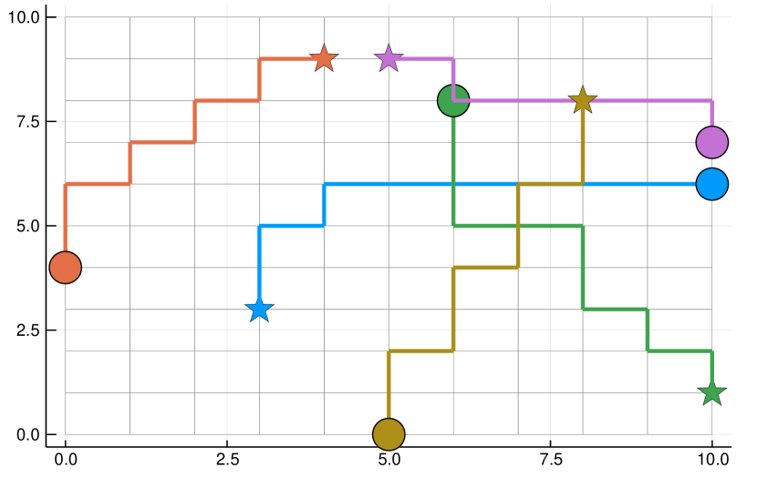
(a) $\epsilon$ = 0.1

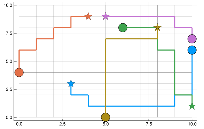
(b) $\epsilon$ = 0.001

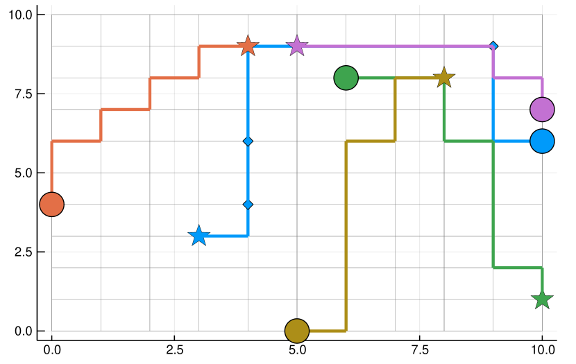
(c) $\epsilon$ = 0.00001

Figure 3: Solutions for STT-CBS on a $10\times 10$ grid for 5 agents, with different values of $\epsilon$. Paths start at the stars, end at the circles, and are paused at the diamonds. With no uncertainty, each edge takes 1 time step to traverse.

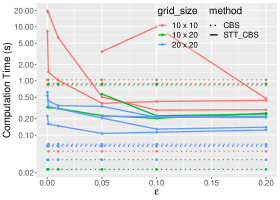
Figure 4: Computation time on a set of random examples for different values of $\epsilon$ on problems with 10 agents and three different grid sizes (time is in logarithmic scale). The dotted lines represent computation times for CBS applied to the same problems. The effect of reducing $\epsilon$, thus increasing problem complexity, is apparent. Whenever $\epsilon$ is sufficiently large, STT-CBS returns the optimal solution within one second. However, the extra control over collision probability comes with a moderately higher computation cost for our STT-CBS, compared with standard CBS.

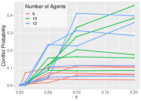
Figure 5: Global conflict probability evaluated for a number of agents varying between 8 and 12. We observe in practice that this value decreases as $\epsilon$ goes to 0.

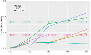
Figure 6: Global conflict probability comparison for randomly selected 10-agent problems. Each color represents a specific trial. Our algorithm gives the user a desired maximum pairwise collision probability $\epsilon$. The conflict probabilities found with CBS are significantly larger than those found with our STT-CBS algorithm for small values of $\epsilon$. The global conflict probability is tied to local pairwise conflict probability (conditioned by $\epsilon$) through the number of interacting agents.

Figure 3 illustrates the effect of $\epsilon$ on the returned solution, for an experiment on a $10\times 10$ grid containing 5 agents. A high value yields a solution very likely to contain conflicts, and if the value is too small, the solution tends to be over-conservative at the expense of a more costly solution. These results are also conditioned by the parameters of the delay distribution of every node.

For all the following experiments, we chose to model delay identically at every node by using parameters $\lambda=5$ and $n_{v}=1$.

Computation time

Figure 4 shows computation time results for CBS and STT-CBS with different values of $\epsilon$. These experiments were performed on $10\times 10$, $10\times 20$ and $20\times 20$ grids and with 10 agents. Whenever the number of iterations surpassed 1000, we interrupted the algorithm and did not represent the corresponding data point in these graphs. It is important to note that while most of these randomly generated problems can be solved within a few seconds, due to the inherent difficulty of the problems solved with each method, neither CBS or STT-CBS provide any computation time guarantees.

Conflict Probability

Figure 5 shows the global conflict probability on a set of experiments as a function of $\epsilon$. We computed the probabilities using Monte Carlo simulation. In these experiments, decreasing $\epsilon$ decreases global conflict probability. Figure 6 compares the results with CBS.

Hardware experiments

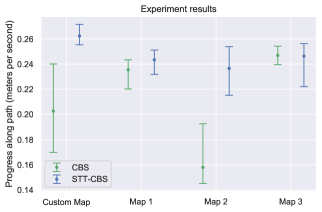
Figure 7: Hardware experiments. For each map and algorithm, 4 trials were conducted. The plot shows the average progress of the robots along their path, in meters per second. This result was obtained by dividing the sum of path lengths by the sum of travel times for all agents. The colored dots represent the mean, and the error bars represent the minimum and maximum sampled values. The collision avoidance algorithm was called while robots executed the CBS solution path in both the Custom Map and Map 2 due to robots navigating too closely to each other, resulting in slower progress over these trials. We find that that the additional safety provided by STT-CBS prevented such events to occur. The modeling choices we made in these experiments resulted in slightly longer path lengths, in return for gained predictability in travel time.

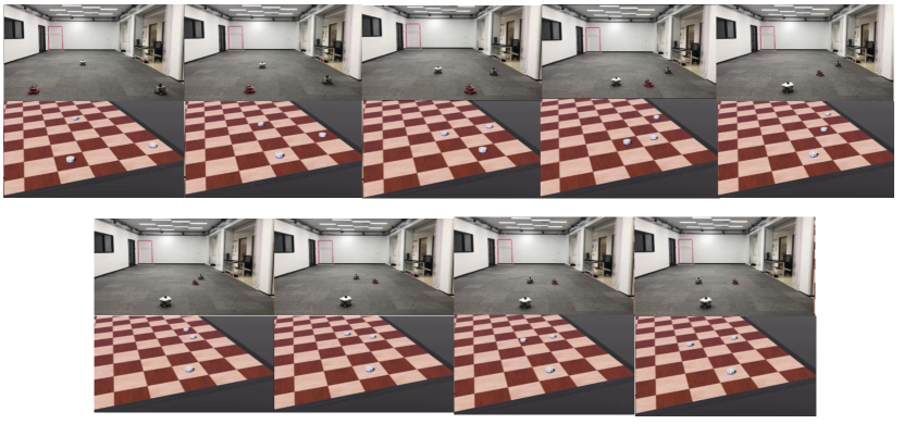
(a) a) STT-CBS

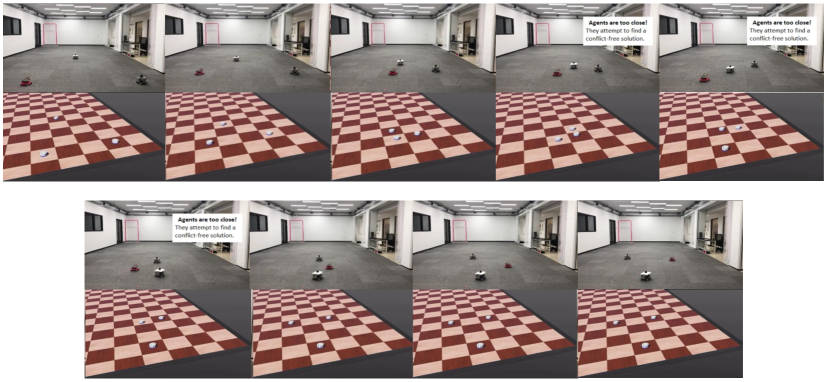
(b) b) CBS

Figure 8: We compare two different solutions computed by STT-CBS and CBS for the same problem in a $5\times 5$ custom environment. At each time step, we compare agents’ actual (upper) and simulated (lower) positions. We notice that the solution returned by CBS requires the agents to navigate close to one another as they follow each other. During the execution, agents are not able to perform this maneuver without risking collision and compute alternate routes to avoid each other. In contrast, STT-CBS returns a slightly more expensive solution that the agents are able to execute safely.

In order to test our algorithm, we use the OuijaBot [23]—a custom-designed omnidirectional platform—to execute solutions. To avoid collisions, we plan trajectories using Reciprocal Collision Avoidance for Real-Time Multi-Agent Simulation [20]. In the experiments, three robots are instructed to follow way-points. Travel time is uncertain as their dynamics vary with time, battery level, and floor condition, and they may need to manoeuvre around each other. The distribution for agent delay is unknown and realistic.

We compare the performance of CBS and STT-CBS in one custom environment, and three chosen among 10 randomly generated environments where CBS and STT-CBS yield different solutions. We chose $n_{v}=1$ and $\lambda=5$ at all nodes to model delay, and $\epsilon=0.1$ as conflict probability threshold. The results are summarized in Figure 7. Figure 8 illustrates a difficulty that becomes apparent when the computed path is not sufficiently robust to travel time uncertainty. We notice that the solution generated by CBS for the custom environment requires the agents to navigate close to one another as they follow each other. During execution, agents fail to perform this maneuver without risking collision and compute alternate routes to avoid each other. In contrast, STT-CBS returns a more expensive solution that the agents are able to execute safely.

6 Conclusion

STT-CBS offers quantifiable robustness to stochastic travel time delays in realistic multi-agent path finding scenarios compared with the standard CBS method, while minimizing the expected solution cost. An interesting direction for future work is the integration of stochastic travel time models into other path planning algorithms, such as some of the many variants and extensions of Conflict-Based Search [8, 13, 10, 4]. In addition, the multi-agent path planning literature will benefit from a comparison of different ‘robust’ MAPF solvers in both realistic simulations and hardware experiments.

References

- [1] Jalal Ashayeri and LF Gelders “Warehouse design optimization” In European Journal of Operational Research 21.3 Elsevier, 1985, pp. 285–294
- [2] Dor Atzmon et al. “Probabilistic robust multi-agent path finding” In International Conference on Automated Planning and Scheduling (ICAPS) 30, 2020, pp. 29–37
- [3] Dor Atzmon et al. “Robust Multi-Agent Path Finding” In International Conference on Autonomous Agents and Multiagent Systems (AAMAS) Stockholm, Sweden: International Foundation for Autonomous AgentsMultiagent Systems, 2018, pp. 1862–1864 URL: http://dl.acm.org/citation.cfm?id=3237383.3238004
- [4] Kyle Brown et al. “Optimal Sequential Task Assignment and Path Finding for Multi-Agent Robotic Assembly Planning” In IEEE International Conference on Robotics and Automation (ICRA), 2020, pp. 441–447 DOI: 10.1109/ICRA40945.2020.9197527
- [5] Boris De Wilde, Adriaan W. Ter Mors and Cees Witteveen “Push and Rotate: A Complete Multi-agent Pathfinding Algorithm” In Journal of Artificial Intelligence Research 51.1 USA: AI Access Foundation, 2014, pp. 443–492 URL: http://dl.acm.org/citation.cfm?id=2750423.2750435
- [6] Ariel Felner et al. “Adding Heuristics to Conflict-Based Search for Multi-Agent Path Finding” In International Conference on Automated Planning and Scheduling (ICAPS), 2018
- [7] F. Ho et al. “Improved Conflict Detection and Resolution for Service UAVs in Shared Airspace” In IEEE Transactions on Vehicular Technology 68.2, 2019, pp. 1231–1242
- [8] Wolfgang Hönig et al. “Conflict-Based Search with Optimal Task Assignment” In International Conference on Autonomous Agents and Multiagent Systems (AAMAS), 2018 URL: http://dl.acm.org/citation.cfm?id=3237383.3237495
- [9] D.. Kornhauser “COORDINATING PEBBLE MOTION ON GRAPHS, THE DIAMETER OF PERMUTATION GROUPS, AND APPLICATIONS” Cambridge, MA, USA: Massachusetts Institute of Technology, 1984
- [10] Jiaoyang Li et al. “Disjoint splitting for multi-agent path finding with conflict-based search” In International Conference on Automated Planning and Scheduling (ICAPS), 2019, pp. 279–283
- [11] Jiaoyang Li et al. “Multi-Agent Path Finding for Large Agents” In AAAI Conference on Artificial Intelligence (AAAI), 2019, pp. 7627–7634 DOI: 10.1609/aaai.v33i01.33017627
- [12] V.J. Lumelsky and K.R. Harinarayan “Decentralized Motion Planning for Multiple Mobile Robots: The Cocktail Party Model” In Autonomous Robots 4, 1997, pp. 121–135 DOI: 10.1023/A:1008815304810
- [13] Hang Ma and Sven Koenig “Optimal Target Assignment and Path Finding for Teams of Agents” In International Conference on Autonomous Agents and Multiagent Systems (AAMAS), 2016, pp. 1144–1152
- [14] Hang Ma, TK Satish Kumar and Sven Koenig “Multi-agent path finding with delay probabilities” In AAAI Conference on Artificial Intelligence (AAAI), 2017, pp. 3605–3612
- [15] S. Samaranayake, S. Blandin and A. Bayen “A tractable class of algorithms for reliable routing in stochastic networks” In Transportation Research Part C: Emerging Technologies 20.1, 2012, pp. 199–217 DOI: https://doi.org/10.1016/j.trc.2011.05.009
- [16] Tomer Shahar et al. “Safe Multi-Agent Pathfinding with Time Uncertainty” In Journal of Artificial Intelligence Research 70, 2021, pp. 923–954
- [17] G. Sharon, R. Stern, A. Felner and N.R. Sturtevant “Conflict-Based Search for Optimal Multi-Agent Path Finding” In Artificial Intelligence 219, 2012, pp. 40–66
- [18] Trevor Standley and Richard Korf “Complete Algorithms for Cooperative Pathfinding Problems” In International Joint Conference on Artificial Intelligence (IJCAI) Barcelona, Catalonia, Spain: AAAI Press, 2011, pp. 668–673 DOI: 10.5591/978-1-57735-516-8/IJCAI11-118
- [19] Pavel Surynek “Unifying search-based and compilation-based approaches to multi-agent path finding through satisfiability modulo theories” In International Joint Conference on Artificial Intelligence (IJCAI), 2019, pp. 1177–1183 AAAI Press
- [20] Jur Van Den Berg, Stephen J. Guy, Ming Lin and Dinesh Manocha “Reciprocal n-Body Collision Avoidance” In Robotics Research Berlin, Heidelberg: Springer Berlin Heidelberg, 2011, pp. 3–19
- [21] Glenn Wagner and Howie Choset “M*: A Complete Multirobot Path Planning Algorithm with Optimality Bounds” In Redundancy in Robot Manipulators and Multi-Robot Systems Berlin, Heidelberg: Springer Berlin Heidelberg, 2013, pp. 167–181 DOI: 10.1007/978-3-642-33971-4˙10
- [22] Glenn Wagner and Howie Choset “Path Planning for Multiple Agents under Uncertainty” In International Conference on Automated Planning and Scheduling (ICAPS), 2017
- [23] Zijian Wang, Guang Yang, Xuanshuo Su and Mac Schwager “OuijaBots: Omnidirectional Robots for Cooperative Object Transport with Rotation Control Using No Communication” In International Symposium on Distributed Autonomous Robotic Systems, 2016, pp. 117–131 DOI: 10.1007/978-3-319-73008-0“˙9
- [24] Peter Wurman, Raffaello D’Andrea and Mick Mountz “Coordinating Hundreds of Cooperative, Autonomous Vehicles in Warehouses.” In AI Magazine 29, 2008, pp. 9–20
- [25] J. Yu and S.. LaValle “Optimal Multirobot Path Planning on Graphs: Complete Algorithms and Effective Heuristics” In IEEE Transactions on Robotics 32.5, 2016, pp. 1163–1177 DOI: 10.1109/TRO.2016.2593448
- [26] Jingjin Yu and Steven LaValle “Structure and Intractability of Optimal Multi-Robot Path Planning on Graphs” In AAAI Conference on Artificial Intelligence (AAAI), 2013