Improved axion haloscope search analysis

Abstract

One of the most significant and practical figures of merit in axion haloscope searches is the scanning rate, because of the unknown axion mass. Under the best experimental parameters, the only way to improve the figure of merit is to increase the experimentally designed signal to noise ratio in the axion haloscope search analysis procedure. In this paper, we report an improved axion haloscope search analysis using the data taken by the CAPP-8TB haloscope. By correcting for the background biased by the background parametrizations in the presence of axion signals, we realized a signal to noise ratio efficiency of about 100%. Given the axion haloscope search analyses to date, the scanning rate can be improved by 21%, with about a 10% improvement in the signal to noise ratio. This improvement is another low cost innovation in axion haloscope searches, where all the experimental parameters are currently at their best.

1 Introduction

The axion AXION is an elementary particle considered to result from a breakdown in a new symmetry first proposed by Peccei and Quinn (PQ symmetry) PQ to solve the strong $CP$ problem in the Standard Model of particle physics  strongCP . This particle is massive, stable, and is born cold by the PQ symmetry breaking. This makes the axion one of the most promising candidates for cold dark matter, which constitutes about 85% of the matter in the Universe according to cosmological measurements and the standard model of Big Bang cosmology PLANCK .

The method of searching for the axion proposed by Sikivie sikivie , also known as the axion haloscope search, involves a microwave resonant cavity with a strong static magnetic field that induces axions to convert into microwave photons. Using the resonant cavity, the axion signal power can be enhanced when the axion mass $m_{a}$ matches the resonant frequency of the cavity mode $\nu$, $m_{a}=h\nu/c^{2}$. Because the axion mass is unknown, however, the resonant cavity has to be tunable, to allow axion haloscope searches to scan all frequencies corresponding to possible axion masses. Because of this frequency scanning procedure, the most significant and practical figure of merit in axion haloscope searches is the scanning rate scanrate

$$\frac{d\nu}{dt}=\frac{\nu b_{a}}{Q_{L}}\Big{(}\frac{1}{\rm SNR_{target}}\Big{)}^{2}\Big{(}\frac{P^{a\gamma\gamma}_{a}}{P_{n}}\Big{)}^{2}\propto\frac{g^{4}_{a\gamma\gamma}B^{4}V^{2}C^{2}Q_{L}}{{\rm SNR^{2}_{target}}T^{2}_{n}}$$ (1)

for a target signal to noise ratio ${\rm SNR_{target}}$. $P^{a\gamma\gamma}_{a}$ is the axion signal power proportional to $g^{2}_{a\gamma\gamma}B^{2}VCQ_{L}$ sikivie ; scanrate , where $g_{a\gamma\gamma}$ is the axion-photon coupling strength, $B$ is a static magnetic field provided by magnets in the axion haloscopes, $V$ is the cavity volume, $C$ is a form factor representing the overlap between the electric field of the cavity mode and the static magnetic field whose general definition can be found in Ref. EMFF_BRKO , and $Q_{L}$ is the loaded quality factor of the cavity mode. $P_{n}$ is the noise power proportional to the noise temperature $T_{n}$ and the axion signal window $b_{a}$.

From the radiometer equation DICKE , the SNR is

$${\rm SNR_{designed}}=\frac{P^{a\gamma\gamma}_{a}}{\sigma_{P_{n}}},$$ (2)

where $\sigma_{P_{n}}$ is the noise power fluctuation. The subscript “designed” stands for experimentally designed, thus the ${\rm SNR_{designed}}$ must be designed to be the same as the $\rm SNR_{target}$ or the $\rm SNR_{target}$ must be set to be the ${\rm SNR_{designed}}$ in order to have an axion haloscope search in an experimentally designed time. However, generally the experimentally achieved signal to noise ratio ${\rm SNR_{achieved}}$ is smaller than the designed one by holding the relation ${\rm SNR_{achieved}}=\epsilon_{\rm SNR}{\rm SNR_{designed}}$, where $\epsilon_{\rm SNR}$ is the reconstruction efficiency of the ${\rm SNR_{designed}}$ in an axion haloscope search analysis procedure whose values vary from about 50 to 90% depending on the analysis strategy ADMX ; HAYSTAC ; simple_ACTION .

Having said that, the scanning rate guides the following two cases.

1. For axion haloscope searches to achieve the target sensitivity or ${\rm SNR_{target}}$ in an experimentally designed time, the experimental parameters, $B$, $V$, $C$, $Q_{L}$, and $T_{n}$ have to be designed to meet the condition ${\rm SNR_{achieved}}={\rm SNR_{target}}$,

2. For axion haloscope searches to achieve the target sensitivity or ${\rm SNR_{target}}$, axion haloscopes have to take data until the condition ${\rm SNR_{achieved}}={\rm SNR_{target}}$ is satisfied, even under the experimental parameters, $B$, $V$, $C$, $Q_{L}$, and $T_{n}$ at their best.

In both cases, the figure of merit of the experiments can be enhanced by improving the ${\rm SNR_{achieved}}$ or $\epsilon_{\rm SNR}$, which results in more sensitive results for (I) and shorter data acquisition periods for (II).

In this paper, we report an improved axion haloscope search analysis using the data taken by the CAPP-8TB haloscope CAPP-8TB-PRL . Using the improved axion haloscope search analysis in this paper, the figure of merit of axion haloscope searches can be effectively increased by about 21%.

2 Axion haloscope search analysis strategy

The simplest axion haloscope search analysis strategy is the one-bin search that was employed in Ref. simple_ACTION , where all the axion signal power belongs to a single frequency bin width corresponding to the axion signal window $b_{a}$, if axions are there. The price for the simplicity of this one-bin search is a very low reconstruction efficiency of the axion signal power $\epsilon_{P^{a\gamma\gamma}_{a}}$. As described in Refs. ADMX ; simple_ACTION , we lose about 20% of the signal power by choosing a signal window to get an optimized SNR, and an additional 20% from the frequency binning choice.

The other strategy is the multi-bin co-adding search developed by the Axion Dark Matter eXperiment (ADMX) ADMX , where all the axion signal power is distributed over the multi frequency bins obeying an axion signal shape turner (also shown in Fig. 1). The multi frequency bin width also corresponds to the axion signal window $b_{a}$. The multi-bin co-adding search overcomes the inefficiency caused by the selection of frequency binning.

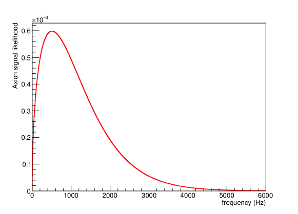
Figure 1: Axion signal likelihood distribution for an axion mass of 1.625 GHz, where the axion mass is downconverted to zero. We can retain about 99.9% of the total signal power by taking the signal window of 5000 Hz or, equivalently, 10 frequency bins with a resolution bandwidth of 500 Hz.

The multi-bin co-adding search with signal likelihood weighting developed by the Haloscope At Yale Sensitive To Axion Cold dark matter (HAYSTAC) HAYSTAC overcomes the inefficiency resulting from the choice of signal window.

As reported in ADMX ; HAYSTAC ; simple_ACTION , however, the background subtraction with a 5-parameter fit ADMX ; simple_ACTION or a Savitzky-Golay filter HAYSTAC also generates an additional inefficiency of about 20% in the SNR reconstruction in the axion haloscope search analysis procedure. The HAYSTAC analysis procedure recovered this inefficiency using a single frequency-independent numerical factor, resulting in an improvement of about 8% in $\epsilon_{\operatorname{SNR}}$ HAYSTAC . Another low cost innovation in axion haloscope searches might be to improve the inefficiency induced by the background subtraction, and that is the main contribution of this paper.

3 Axion haloscope search analysis procedure

The axion haloscope search analysis procedure can be divided into the following three steps:

1. Step-1 ; background parametrization for the background subtraction,

2. Step-2 ; combining all the power spectra as a single power spectrum, taking into account the overlaps among the power spectra,

3. Step-3 ; constructing a “grand power spectrum” by co-adding multi-bins with signal likelihood weighting.

After the background subtraction in Step-1, the normalized power excess at each stage is likely to follow a Gaussian distribution in the absence of axion signals, because the background in axion haloscope searches is very like stationary Poisson noise. The mean of the Gaussian depends on the expected SNR, while its width should be unity if the power excess errors are estimated correctly. All of the effort in this work is focused on obtaining such a Gaussian distribution in each step, from Step-1 to Step-3.

4 Data and parameters

Here we describe the data used for this work. It consists of:

1. experimental data from the CAPP-8TB experiment CAPP-8TB-PRL ,

2. 5000 simulated axion haloscope search experiments with a flat background and axion signals at a particular frequency, referred to as “flat background simulation data”,

3. 5000 simulated axion haloscope search experiments with the CAPP-8TB backgrounds and axion signals at a particular frequency, referred to as “CAPP-8TB simulation data”,

4. 5000 simulated axion haloscope search experiments with the CAPP-8TB backgrounds only, referred to as “background only simulation data”,

5. other 4 sets of 5000 simulated axion haloscope search experiments with the CAPP-8TB backgrounds, where each set has axion signals at different frequencies, thus has different SNRs, referred to as “other CAPP-8TB simulation data”.

Here we also employ some assumptions and parameters adopted by the CAPP-8TB axion haloscope search CAPP-8TB-PRL . We assume the axions have an isothermal distribution, thus distribute over a boosted Maxwellian shape, as shown in Fig. 1, with the following parameters: an axion rms velocity of about 270 km/s and the Earth rms velocity of 230 km/s with respect to the galaxy frame turner . We took 5000 Hz as the signal window of the axions considered in CAPP-8TB. We can then retain about 99.9% of the total signal power as shown in Fig. 1. After Step-1, the five nonoverlapping frequency bins in each background-subtracted power spectrum were merged so that the resolution bandwidth (RBW) became 500 Hz, which we refer to as “Step-1.5”. An RBW of 500 Hz was chosen not only to retain the axion signal shape shown in Fig. 1, but also to avoid unnecessarily inordinate calculation time. The Step-2 and Step-3 procedures then went through with the RBW of 500 Hz CAPP-8TB-PRL . With our 10 co-adding bins in Step-3, therefore, $P^{a\gamma\gamma}_{a}$ is almost 100% retained.

5 Validations

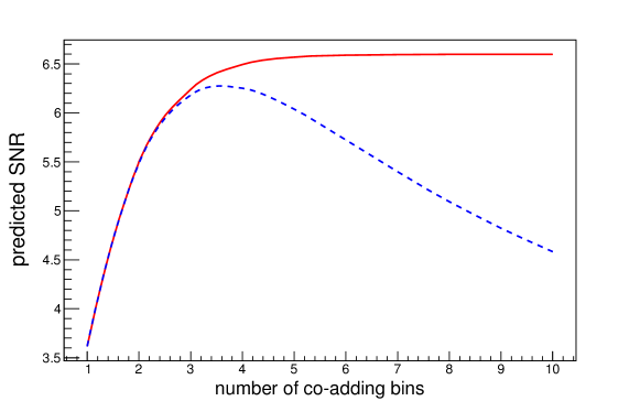
Figure 2: Predicted SNR as a function of the number of co-adding bins. Solid (red) and dashed (blue) lines show SNRs with and without the signal weighting applied, respectively.

Using the flat background simulation data, first, we validated our understanding of the axion haloscope search analysis procedure, especially the signal weighting in the Step-3 procedure as well as our simulation data, particularly the signal injections that must reflect our cavity responses. With a flat background, one can easily predict solid SNRs with little background dependence in the Step-2 procedure. Figure 2 shows the predicted SNR as a function of the number of co-adding bins with and without the signal weighting. The weighting factors were obtained by integrating over the relevant regions of the axion signal likelihood shown in Fig. 1.

The flat background simulation data was fed through the procedure described in Sec. 3. The backgrounds were subtracted without any fit parametrizations. All the background-subtracted power spectra were then combined as a single power spectrum. In constructing a grand power spectrum, each power spectral line in the single power spectrum was weighted accordingly HAYSTAC using the axion signal likelihood shown in Fig. 1.

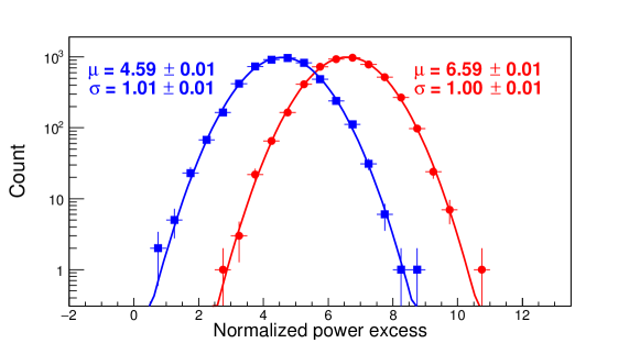
Figure 3: Distributions of the normalized power excess from a particular frequency bin where we put simulated axion signals, with (circles) and without (rectangles) the signal weighting applied. Lines are a Gaussian fit.

It was further normalized by the corresponding noise fluctuation, which was also weighted according to the axion signal shape HAYSTAC . With a signal window of 5000 Hz or, equivalently, 10 co-adding bins, Fig. 3 shows two distributions of the normalized power excess from a particular frequency where we put simulated axion signals, with (circles) and without (rectangles) the signal weighting, respectively. Figure 3 also shows the Gaussian fit results, including the means ($\mu$) and widths ($\sigma$) of the distributions. Both means follow the predicted SNRs shown in Fig. 2 and the widths are unity as they should be.

Having demonstrated our solid understanding of the simulation data and axion haloscope search analysis procedure from the flat background simulation data, we applied the same analysis procedure to the CAPP-8TB simulation data as well as the CAPP-8TB experimental data, but with a 5-parameter fit ADMX for the background parametrization and subtraction. The same procedure except for the background subtraction using the simulation input background functions, i.e., a perfect fit, was also applied just to the simulation data to determine the inefficiency resulting from the background subtraction ADMX ; HAYSTAC ; simple_ACTION .

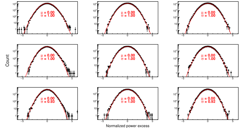
Figure 4: Distributions of the normalized power excess from the CAPP-8TB experiment (triangles in the 1st column), and from a single simulated axion haloscope search experiment with CAPP-8TB backgrounds and axion signals at a particular frequency (inverted triangles in the 2nd and 3rd columns). Distributions in the 2nd column were obtained after subtracting the background with perfect fit, while those in the 1st and 3rd columns were with a 5-parameter fit. From top to bottom row, they are the distributions after the Step-1, Step-2, and Step-3 procedures, respectively. Lines are a Gaussian fit resulting in $\mu$ and $\sigma$ with negligible fit errors of $\mathcal{O}(10^{-3})$ SMALLERROR .

The normalized power excess distributions from the CAPP-8TB experimental data are shown as triangles in the 1st column of Fig. 4. The distributions from a single simulated axion haloscope search experiment with CAPP-8TB backgrounds and axion signals at a particular frequency are shown in the 2nd and 3rd columns of Fig. 4 as inverted triangles. The distributions in the 1st and 3rd columns were obtained after subtracting the background with a 5-parameter fit, while in the 2nd they were obtained with a perfect fit. From top to bottom, they are the distributions after the Step-1, Step-2, and Step-3 procedures, respectively. The distributions after the Step-3 procedure are narrower than unity for both the experimental and simulation data with a 5-parameter background parametrization. This has been previously observed in axion haloscope search experiments ADMX ; HAYSTAC ; simple_ACTION . Without shrinking the distribution after the Step-3 procedure with perfect fit (bottom center of Fig. 4), the narrower width of the normalized power excess distribution must be induced from the background parametrization and subtraction thereafter ADMX ; HAYSTAC ; simple_ACTION .

Our validations shown in Figs. 3 and 4 demonstrate not only our solid understanding of the analysis procedure but also the validity of our simulation data.

6 Incorporating the full correlations

Equation (3) shows the power excess in one of the frequency bins of the grand power spectrum with the signal weighting HAYSTAC

$$P_{{\operatorname{g}}}=\sum_{i=1}^{\begin{subarray}{c}{\operatorname{co-adding}}\\ {\operatorname{bins}}\end{subarray}}P_{i}\mathcal{L}_{i}$$ (3)

and Eq. (4) shows the full error propagation of the power excess shown in Eq. (3)

$$\sigma^{2}_{P_{{\operatorname{g}}}}=\sum_{i=1}^{\begin{subarray}{c}{\operatorname{co-adding}}\\ {\operatorname{bins}}\end{subarray}}\sum_{j=1}^{\begin{subarray}{c}{\operatorname{co-adding}}\\ {\operatorname{bins}}\end{subarray}}\sigma_{P_{i}}\sigma_{P_{j}}\mathcal{L}_{i}\mathcal{L}_{j}\rho_{ij},$$ (4)

where $P_{i}$ and $\sigma_{P_{i}}$ are the power excess and associated error in the $i_{\rm th}$ frequency bin of the combined power spectrum after the Step-2 procedure, respectively, and $\mathcal{L}_{i}$ is an axion signal likelihood for both the $P_{i}$ and $\sigma_{P_{i}}$ weightings. With the signal window $b_{a}$ of 5000 Hz as shown in Fig. 1, $\mathcal{L}_{i}$ meets the condition $\sum_{i=1}^{\begin{subarray}{c}{\operatorname{co-adding}}\\ {\operatorname{bins}}\end{subarray}}\mathcal{L}_{i}\simeq 1$ with 10 co-adding frequency bins and an RBW of 500 Hz for the CAPP-8TB axion haloscope search. $\rho_{ij}$ is the correlation coefficient between the frequency bins participating in the co-adding procedure, thus is unity for $i=j$. The narrower width of the normalized power excess distribution from the normalized grand power spectrum could mean that the noise fluctuations in the grand power spectrum $\sigma_{P_{\operatorname{g}}}$ are overestimated with the terms for $i=j$ only in Eq. (4) or, equivalently, with $\sum_{i=1}^{\begin{subarray}{c}{\operatorname{co-adding}}\\ {\operatorname{bins}}\end{subarray}}\sigma^{2}_{P_{i}}\mathcal{L}^{2}_{i}$ only. The correlation coefficients $\rho_{ij}$ in Eq. (4) are very likely to be negative due to overestimation of the noise fluctuations in the grand power spectrum ADMX ; HAYSTAC ; simple_ACTION .

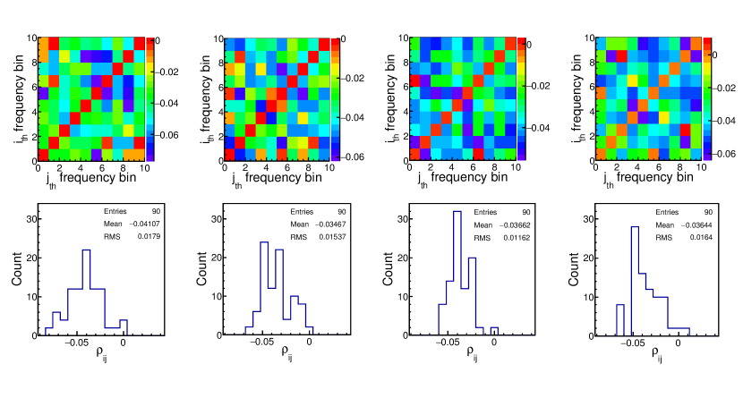
Figure 5: Examples of the correlation coefficient maps (top) and the projections onto the correlation coefficient axis (bottom). In the top 2-D plots, $\rho_{ij}$ for $i=j$ are unity with 100% correlation, but are set to zero to distinguish the differences among $\rho_{ij}$ for $i\neq j$. $\rho_{ij}$ for $i=j$ are also left out in the bottom histograms and that is the reason the entries in them are not 100, but 90 from a 10$\times$10 matrix. Plots in the 1st column were obtained from a frequency that has axion signals, and those in the next three columns from other frequencies with no axion signals.

With 10 co-adding bins, each frequency bin in the grand power spectrum has a full error contribution from $10\times 10$ combinations or, equivalently, from a relevant $10\times 10$ correlation matrix. The total number of frequencies in our grand power spectrum is 100001 with a frequency band of 50 MHz (1600 to 1650 MHz) and an RBW of 500 Hz CAPP-8TB-PRL , hence we need to construct 100001 $10\times 10$ correlation matrices. These 100001 correlation matrices were constructed from the CAPP-8TB simulation data and background only simulation data. The elements in each correlation matrix were calculated as the standard Pearson correlation coefficient. The CAPP-8TB simulation data was used for the background parametrizations and the parametrizations were then applied to the background only simulation data to extract the power excess for the correlation coefficient calculations. Figure 5 shows examples of the correlations obtained from the simulation data. The 1st column shows the correlation coefficient map and the distribution of the correlation coefficients from a frequency that has input axion signals, and the other columns show them from frequencies that have no axion signals. As predicted earlier, most of the correlation coefficients were constructed as negative values, which can explain the narrower widths of the normalized power excess distributions shown in the bottom left (experimental data) and right (simulation data) of Fig. 4.

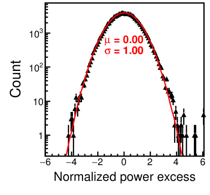
Figure 6: The figure shows the same data as in the bottom left of Fig. 4 but with the correlation matrices fully incorporated.

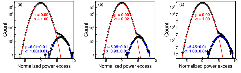
Figure 7: The inverted triangles in (a), (b), and (c) are the distributions of the normalized power excess from all the frequency bins in the normalized grand power spectra from the 5000 simulated CAPP-8TB experiments, while the circles are those from a particular frequency bin where we put simulated axion signals on top of the CAPP-8TB background. (a) was obtained after subtracting the background with perfect fit; (b) and (c) with a 5-parameter fit; (c) incorporates the correlations between the co-adding frequency bins. Lines are a Gaussian fit.

The 100001 correlation matrices constructed from the simulation data were then fed through the CAPP-8TB experimental data and CAPP-8TB simulation data in the Step-3 procedure. Figure 6 was obtained from the CAPP-8TB experimental data CAPP-8TB-PRL , which corresponds to the bottom left data in Fig. 4. After the full incorporation of the correlation matrices the triangles now follow a standard Gaussian distribution.

The results from the CAPP-8TB simulation data are also shown in (a), (b), and (c) in Fig. 7, respectively CAPP-8TB-PRL . Figures 7(a) and 7(b) correspond to the bottom center and right of Fig. 4, respectively, with 5000 simulated CAPP-8TB experiments. Figure 7(c) was also from 5000 simulated CAPP-8TB experiments. Both the inverted triangles and circles follow a Gaussian distribution with a width exhibiting unity, thanks to the full incorporation of the correlation matrices. From the mean values of the circle distributions in Figs. 7(a), 7(b), and 7(c), the SNR efficiencies with a 5-parameter fit are 90.7% and 84.0% with and without the correlation matrices, respectively. The $\epsilon_{\rm SNR}$ of 90.7% with the full frequency-dependent correlations shows good agreement with what the HAYSTAC achieved with a single frequency-independent numerical factor HAYSTAC and was applied to our previous publication CAPP-8TB-PRL . One also can expect such an $\epsilon_{\rm SNR}$ agreement between the HAYSTAC and CAPP-8TB experiments based on Fig. 5, where each correlation coefficient map does not depend significantly on the frequency, or is almost unaffected by the presence of the axion signals.

7 Improvement

Following the HAYSTAC method, the normalized power excess in the Step-3 can be expressed as

$${\operatorname{Normalized~{}grand~{}power~{}excess}}=\frac{P_{\operatorname{grand}}}{\sigma_{P_{\operatorname{grand}}}\xi_{{\operatorname{Step-3}}}},$$ (5)

where $P_{\operatorname{grand}}=P_{\operatorname{g}}$, $\sigma^{2}_{P_{{\operatorname{grand}}}}=\sum_{i=1}^{\begin{subarray}{c}{\operatorname{co-adding}}\\ {\operatorname{bins}}\end{subarray}}\sigma^{2}_{P_{i}}\mathcal{L}^{2}_{i}$, and $\xi_{\operatorname{Step-3}}$ is a frequency-independent scale factor to remedy the bias induced from the background parametrizations. Its value for the CAPP-8TB experiment is 0.92, as shown in Fig. 7(b). Another frequency-independent scale factor $\xi_{\operatorname{Step-1.5}}$ of 0.98 was used in Step-1.5 for the distributions shown in the middle left (experimental data) and right (simulation data) of Fig. 4, hence for the CAPP-8TB results CAPP-8TB-PRL , which is also induced by the background parametrizations. The result using a $\xi_{\operatorname{Step-3}}$ of 0.92 is in good agreement with that using the full correlations. Having said that, through the rest of this work we will employ frequency-independent scale factors.

Equation (5) itself is valid whether the scale factor affects $P_{\operatorname{grand}}$ or $\sigma_{\operatorname{grand}}$, though it was applied to the latter. First, we looked into which are affected by a 5-parameter fit using the CAPP-8TB simulation data. Table 1 shows the category of the normalized grand power excess with different $P_{\operatorname{grand}}$ and $\sigma_{\operatorname{grand}}$ depending mainly on the background parametrizations.

	$P_{\operatorname{grand}}$	$\sigma_{P_{\operatorname{grand}}}$
(A)	perfect fit	perfect fit
(B)	perfect fit	5-parameter fit
(C)	5-parameter fit	perfect fit
(D)	5-parameter fit	5-parameter fit
(E)	5-parameter fit with $\xi_{\operatorname{Step-1.5}}$	5-parameter fit
(F)	5-parameter fit with $\xi_{\operatorname{Step-1.5}}$ and $\xi_{\operatorname{Step-3}}$	5-parameter fit

Table 1: (A) to (F) is the category of the normalized grand power excess with different $P_{\operatorname{grand}}$ and $\sigma_{\operatorname{grand}}$ depending mainly on the background parametrizations.

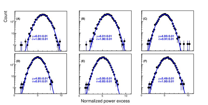
Figure 8: Normalized grand power excess distributions from the 5000 simulated CAPP-8TB experiments at the simulated axion signal frequency, where the conditions for (A) to (F) are listed in Table 1. Lines are a Gaussian fit resulting in $\mu$ and $\sigma$.

Figure 8 shows the normalized grand power excess distributions at the simulated axion signal frequency, where they are categorized according to Table 1. Since we found the 5-parameter fit actually affects only $P_{\operatorname{grand}}$ from the simulation study shown in Table 1 and Fig. 8, we will correct for $P_{\operatorname{grand}}$ only to improve $\epsilon_{\rm SNR}$.

Second, we scrutinized the signal region and found that the 5-parameter fit little affects the axion signal power, but mainly distorts the background in the presence of the axion signals. The dashed lines in Fig. 9 are the $P_{\operatorname{grand}}$ difference between (C) and (A) in Table 1 and show no axion signal excess, which implies the axion signal power identified using the 5-parameter fit and perfect fit are the same. The solid line in Fig. 9 is the $P_{\operatorname{grand}}$ difference between (F) and (A) in Table 1 and the axion signal excess is not due to the 5-parameter fit, but due to the two frequency-independent scale factors $\xi_{\operatorname{Step-1.5}}$ and $\xi_{\operatorname{Step-3}}$, which can result in overestimated SNRs. The difference between the dashed and solid lines in the axion signal sideband regions are also due to $\xi_{\operatorname{Step-1.5}}$ and $\xi_{\operatorname{Step-3}}$.

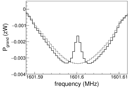
Figure 9: Differences between $P^{\operatorname{5-parameter~{}fit}}_{\operatorname{grand}}$ and $P^{\operatorname{perfect~{}fit}}_{\operatorname{grand}}$, where the former was obtained with 5-parameter fit and the latter with perfect fit. The dashed line was obtained without $\xi_{\operatorname{Step-1.5}}$ and $\xi_{\operatorname{Step-3}}$, while the solid line reflects the two frequency-independent scale factors.

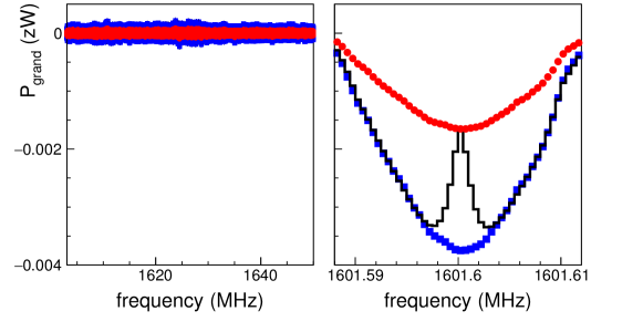
Figure 10: Rectangles (blue) and circles (red) are the underestimated and scaled background corrections, respectively, obtained from the CAPP-8TB simulation data and background only simulation data. Left and right show the corrections in the frequency regions without and with the simulated axion signals, respectively, and the solid line (black) on the right is the same as the solid line in Fig. 9.

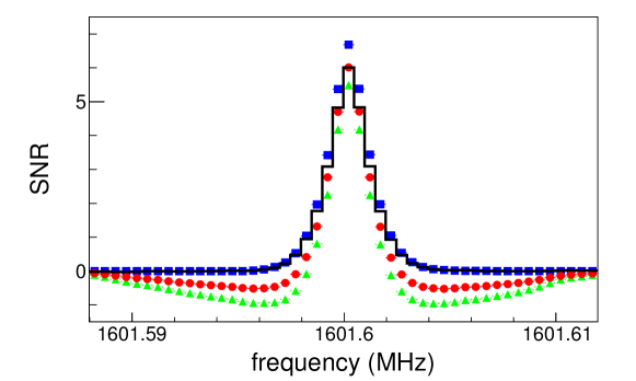
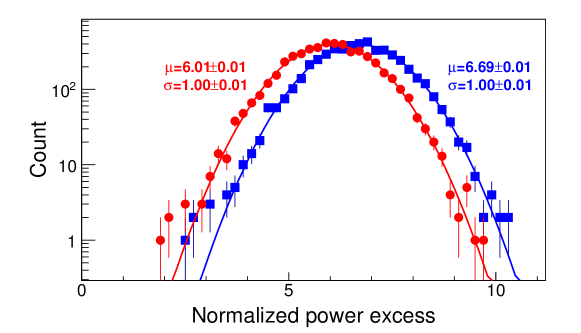
Figure 11: Top shows the final SNRs after the Step-3 procedure, as a function of frequency around the signal region only, from 5000 simulated CAPP-8TB experiments. The line (black) was obtained with perfect fit, triangles (green) with 5-parameter fit without any background corrections, rectangles (blue) with 5-parameter fit with the underestimated background correction, and circles (red) with 5-parameter fit with the scaled background correction, respectively. The circles and rectangles in the bottom plot are the projections of the circle and rectangle of the top plot at the signal frequency which shows the best SNR. Other projections of the line and triangle of the top plot in the signal frequency correspond to (A) and (F) in Fig. 8, respectively. Lines in the bottom plot are a Gaussian fit resulting in $\mu$ and $\sigma$.

We corrected for the background biased by the background parametrizations in the presence of axion signals using the CAPP-8TB simulation data and background only simulation data. The CAPP-8TB simulation data was used for the background parametrizations. The parametrizations were then applied to the background only simulation data to extract the background corrections shown as rectangles (blue) in Fig. 10, which are actually the power excess for the correlation coefficient calculations in Sec. 6, after further going through the Step-3 procedure. However, the background correction using the rectangles in Fig. 10 cannot suppress the overestimated axion signal excess, which is shown in Figs. 9 and 10 by the solid line. This can result in overestimated SNRs as mentioned earlier. Hence we refer to the correction as “underestimated background correction”. To avoid the overestimated axion signal excess, we applied another scale factor $\zeta$ of 0.44 to the underestimated background correction, which is shown in Fig. 10 as circles (red) which are referred to as “scaled background correction”. The scale factor of 0.44 was obtained at the axion signal frequency by equating the difference between the two background corrections (rectangles and circles in Fig. 10) and the overestimated axion signal excess (solid line in Fig. 9), where the scaled background correction is the product of the scale factor and the underestimated background correction. The left and right plots in Fig. 10 show the background corrections in the frequency regions without and with the simulated axion signals, respectively. The narrower band with circles (red) in the left plot resulted from the scale factor $\zeta$. Note that the noise power with the co-adding and signal weighting is about 6.5 zW in the signal region, thus the scaled background correction is at most 0.03% of the noise power. The underestimated background correction is at most 0.06% of the noise power, which can explain why the $\sigma_{\operatorname{grand}}$ from the 5-parameter fit has no problems, as shown in Fig. 8(B). Figure 11 shows the SNRs after applying the two background corrections, where rectangles (blue) are SNRs with the underestimated background correction and circles (red) are those with the scaled background correction. The SNR using the scaled background correction shows good agreement with that using perfect fit (solid line) in the axion signal frequency, while the SNR with the underestimated background correction is overestimated by a factor of $1/(\xi_{\operatorname{Step-1.5}}\xi_{\operatorname{Step-3}})$, as shown in the bottom plot of Fig. 11, as expected earlier. Finally, we confirmed that the scale factor $\zeta$ is a frequency-independent numerical factor from the other CAPP-8TB simulation data, which has to be. Otherwise, the direction of the background correction in this paper is undesirable for axion haloscope searches because of the unknown axion mass.

8 Summary

We report an approach to improve axion haloscope search analyses using the data obtained with the CAPP-8TB haloscope. By correcting for the background biased by the background parametrizations in the presence of axion signals, we realized an $\epsilon_{\operatorname{SNR}}$ of about 100%. Given the axion haloscope search analyses to date, the scanning rate can be improved by 21%, with about a 10% improvement in the SNR. For the CAPP-8TB results CAPP-8TB-PRL , the limits of $g_{a\gamma\gamma}$ can be improved by about 5% with an improved $\epsilon_{\rm SNR}$, e.g., from about 1.00$\times 10^{-14}$ to 0.95$\times 10^{-14}$ GeV^-1. This improvement is another low cost innovation in axion haloscope searches, where all the experimental parameters are currently at their best.

- (1) S. Weinberg, Phys. Rev. Lett. 40 (1978) 223; F. Wilczek, Phys. Rev. Lett. 40 (1978) 279.
- (2) R. D. Peccei and H. R. Quinn, Phys. Rev. Lett. 38 (1977) 1440.
- (3) G. ’t Hooft, Phys. Rev. Lett, 37 (1976) 8; Phys. Rev. D 14 (1976) 3432; 18 (1978) 2199(E); J. H. Smith, E. M. Purcell, and N. F. Ramsey, Phys. Rev. 108 (1957) 120; W. B. Dress, P. D. Miller, J. M. Pendlebury, P. Perrin, and N. F. Ramsey, Phys. Rev. D 15 (1977) 9; I. S. Altarev et al., Nucl. Phys. A341 (1980) 269.
- (4) P. A. R. Ade et al. (Planck Collaboration), Astron. Astrophys. 594 (2016) A13.
- (5) P. Sikivie, Phys. Rev. Lett. 51 (1983) 1415; Phys. Rev. D 32 (1985) 2988.
- (6) L. Krauss, J. Moody, F. Wilczek, and D. E. Morris, Phys. Rev. Lett. 55 (1985) 1797.
- (7) B. R. Ko et al., Phys. Rev. D 94 (2016) 111702(R).
- (8) R. H. Dicke, Rev. Sci. Instrum. 17 (1946) 268.
- (9) C. Hagmann et al., Phys. Rev. Lett. 80 (1998) 2043; S. J. Asztalos et al., Phys. Rev. D 64 (2001) 092003.
- (10) B. M. Brubaker et al., Phys. Rev. Lett. 118 (2017) 061302; B. M. Brubaker, L. Zhong, S. K. Lamoreaux, K. W. Lehnert, and K. A. van Bibber, Phys. Rev D 96 (2017) 123008.
- (11) J. Choi, H. Themann, M. J. Lee, B. R. Ko, and Y. K. Semertzidis, Phys. Rev. D 96 (2017) 061102(R).
- (12) S. Lee, S. Ahn, J. Choi, B. R. Ko, and Y. K. Semertzidis, Phys. Rev. Lett. 124 (2020) 101802.
- (13) M. S. Turner, Phys. Rev. D 42 (1990) 3572.
- (14) Throughout this paper, negligible fitting errors of were left out.