The PAU Survey: Photometric redshifts using transfer learning from simulations

Abstract

In this paper we introduce the Deepz deep learning photometric redshift (photo-$z$) code. As a test case, we apply the code to the PAU survey (PAUS) data in the COSMOS field. Deepz reduces the $\sigma_{68}$ scatter statistic by 50% at $i_{\rm AB}=22.5$ compared to existing algorithms. This improvement is achieved through various methods, including transfer learning from simulations where the training set consists of simulations as well as observations, which reduces the need for training data. The redshift probability distribution is estimated with a mixture density network (MDN), which produces accurate redshift distributions. Our code includes an autoencoder to reduce noise and extract features from the galaxy SEDs. It also benefits from combining multiple networks, which lowers the photo-$z$ scatter by 10 percent. Furthermore, training with randomly constructed coadded fluxes adds information about individual exposures, reducing the impact of photometric outliers. In addition to opening up the route for higher redshift precision with narrow bands, these machine learning techniques can also be valuable for broad-band surveys.

1 Introduction

Galaxy surveys provide invaluable information for a wide set of science applications. They enable a census of the galaxy population and can constrain cosmological models (Gaztañaga et al., 2012; Weinberg et al., 2013; Eriksen & Gaztañaga, 2015), where the galaxies act as tracers of the underlying dark matter field or are used to measure weak gravitational lensing (Bartelmann & Schneider, 2001; Hoekstra & Jain, 2008). There are two main types of galaxy surveys: spectroscopic and photometric. Spectroscopic surveys have high redshift precision, but for limited galaxy samples. Photometric broad band surveys cover larger volumes and fainter galaxies, but their redshift precision is much lower (Baum, 1962; Koo, 1985; Benítez, 2000; Hildebrandt et al., 2010; Salvato, Ilbert & Hoyle, 2019).

The redshift precision of broad-band surveys is limited by their filter width. An alternative approach is to use narrow-band imaging to obtain high precision redshift estimates for a large sample of galaxies. The Physics of the Accelerating Universe Survey (PAUS) implements this idea using 40 narrow bands spaced uniformly in the optical wavelength range from 4500Å to 8500Å (Padilla et al., 2019). This higher wavelength resolution allows for detecting more features in the spectral energy distribution (SED), leading to a better redshift determination (Martí et al., 2014; Eriksen et al., 2019). For $i_{\rm AB}<22.5$, Eriksen et al. (2019) demonstrated that PAUS attains its intended precision, reaching $\sigma_{z}=0.0037(1+z)$ for a selected 50% of galaxies with secure spectra in zCOSMOS DR3 (Lilly et al., 2007). This precision is about a magnitude better than with a typical broad-band survey.

The redshift estimates by Eriksen et al. (2019) were derived with BCNz2, a template based photometric redshift code tailored to achieve high precision redshifts with PAUS. This code used a linear interpolation between continuum spectral energy density (SED), added additional emission lines and also fitted for zero-points. A global zero-point was determined per band, while the code additionally allowed for a free scaling between the broad and narrow bands per galaxy. The use of a template based code was chosen for two reasons. Initially we needed to derive the redshift for samples of hundreds of galaxies, which are insufficient for training. Furthermore, previous tests on machine learning (ML) codes on simulations had not managed to achieve the target PAUS photo-$z$ precision with a realistic training sample.

Despite theoretically being a versatile method, the BCNz2 template fitting code is hard to extend in different directions (appendix A). For example, the non-linear minimisation was difficult to combine with a model where the individual emission line strengths were varying with correlated priors between the lines. Other difficulties included extending the statistical fitting to also account for photometric outliers (appendix B) or efficiently including priors on the different galaxy types during the minimization. Also, formally one should estimate the redshift by integrating over the space of linear SED combinations and not only consider the minimum (Alarcon in prep.). Together with other difficulties, technical issues have made the template fitting approach hard to develop further. In this paper, we instead investigate applying machine learning techniques to determine PAUS redshifts.

Machine learning redshift determination has a long history, with the ANNz (Collister & Lahav, 2004) neural network code being one of the earliest examples. Furthermore, there are many codes, implementing common machine learning algorithms like neural networks (Skynet) (Bonnett, 2015), support vector machines (SpiderZ) (Jones & Singal, 2017) and tree based codes (tpz) (Kind & Brunner, 2013). Machine learning codes offer certain advantages over template fitting methods. Since the machine learning methods directly map magnitudes and/or colours to redshifts, one is not required to model the SEDs, which can be challenging at high redshifts. For PAUS, the accurate SED modelling started to become a potential limitation for the high redshift precision target. Furthermore, the direct colour-redshift mapping makes the model insensitive to global zero-points.

Constructing the training sample is a central problem to estimate photometric redshifts with machine learning. This sample has been built from precise redshift information from spectroscopic surveys, e.g. zCOSMOS (Lilly et al., 2007) or VIMOS VLT Deep Survey (VVDS) (Le Fèvre et al., 2005). These spectra are also required to cover the colour space (Masters et al., 2015), sampling different types of galaxies. These limited training sets already pose serious problems for broad-band photo-$z$ and become a challenge for a magnitude better photo-$z$ precision that PAUS aims to achieve.

Transfer learning is an approach for reducing the requirement on the training sample (Pan & Yang, 2010). Instead of training the network from scratch, one can start training a network which has previously been trained on different data. The network can even benefit from using networks trained on quite different data. In this paper, we focus on simulations, that resemble the observations. Combining the simulations and data has the ability of reducing the need for training data. While attempted in various forms (e.g. Vanzella et al. 2004; Hoyle et al. 2015), it is not commonly used.

Machine learning techniques can be divided into different categories. The most widely used is supervised learning, which compares a prediction with a label (truth value). Even with dedicated surveys, redshift measurement of the faintest galaxies is considered time consuming (Masters et al., 2019). These surveys usually include tens to hundreds of thousands of spectra for specific targets. By contrast, e.g. the Dark Energy Survey (DES) and Kilo-Degree Survey (KiDS) offer hundreds of millions of galaxies to $i_{\rm AB}<24$, with photometric information. In this paper we study the use of autoencoders, which can be used without knowing the redshift (unsupervised) and has the potential advantage of potentially being able to train using a million of galaxies from PAUS.

This paper is built up in the following manner. First, §2 describes the PAUS data, the network architecture and the training procedure. In §3 we study the usage of transfer learning from simulations. Then §4 shows how autoencoders can be used to reduce the noise. Later in §5 we develop and test a method for including individual exposures. In §6 we validate the redshift probability distributions and introduce quality cuts, and we summarise and conclude in §7.

2 Deep learning photometric redshifts

This paper uses the same input data as Eriksen et al. (2019) (BCNz2) and Cabayol-Garcia et al. (2019). For completeness, §2.1 briefly describes the PAUS data, the external broad bands and the spectroscopic catalogue. In §2.2 we describe the network architecture, in §2.3 the mixture density network to estimate the redshift distributions and in §2.4 the training procedure.

2.1 Input data

This paper focuses on the data from the Cosmological Evolution Survey (COSMOS) field where we have PAUS observations and there are abundant spectroscopic measurements. The COSMOS field also has a large set of photometric surveys, covering the wavelength range from ultra-violet to infrared. Our fiducial setup uses the Canada-France-Hawaii Telescope Lensing Survey (CFHTLenS) $u$-band and the $B,V,r,i,z$ bands from the Subaru telescope as in Eriksen et al. (2019). As the spectroscopic catalogue, we use 8566 secure ($3\leq\rm{CLASS}\leq 5$) redshifts from the zCOSMOS DR3 survey (Lilly et al., 2009) that are observed with all 40 narrow bands.

The PAUS data are acquired at the William Herschel Telescope (WHT) with the PAUCam instrument and transferred to the Port d’Informació Científica (PIC, Tonello et al. 2019). First the images are detrended in the nightly pipeline (Serrano et al. in prep). Our astrometry is relative to Gaia DR2 (Brown et al., 2018), while the photometry is calibrated relative to the Sloan Digital Sky Survey (SDSS) by fitting the Pickles stellar templates (Pickles, 1998) to the $u,g,r,i,z$ broad bands from SDSS (Smith et al., 2002) and then predicting the expected fluxes in the narrow bands. The final zero-points are determined by using the median star zero-point for each image.

PAUS observes weak lensing fields (CFHTLenS: W1, W3 and W4) with deeper broad-band data from external surveys. PAUS uses forced photometry, assuming known galaxy positions, morphologies and sizes from external catalogues. The photometry code determines for each galaxy the radius needed to capture a fixed fraction of light, assuming the galaxy follows a Sérsic profile convolved with a known Point Spread Function (PSF). The algorithm uses apertures that measure 62.5% of the light, since this is considered statistically optimal. A given galaxy is observed several times (3-10) from different overlapping exposures. The coadded fluxes are produced using inverse variance weighting of the individual measurements. As described in §5, we also train the network using individual fluxes.

2.2 Network architecture

For a reminder of the basics of neural networks, we refer the reader to LeCun, Bengio & Hinton (2015). Moreover, Appendix C provides some basics on neural networks and introduces the terminology used in this paper.

Figure 1: The network architecture. Top: The autoencoder, formed by an encoder and a decoder network. The layers are linear and the figure indicates the output dimension. Both networks include 10 layers with 250 nodes. Following the intermediate linear layers are ReLU non-linearities, batchnorm layer and a 2 per cent dropout after all linear layers, except the last three. Bottom: We feed the galaxy flux ratios and the autoencoder features into the photo-$z$ network. Here the layers follow the same structure as the autoencoder, but with 1 per cent dropout after all linear layers. This network is a mixture density network and describe the redshift distribution as a linear mixture of 10 normal distributions.

Figure 1 shows the network architecture of Deepz, which uses a configuration with three linear neural networks. The first two constitute an ‘autoencoder’: a type of unsupervised neural network whose intent is to reduce noise and extract features without knowing the redshift, making it possible to train it with a larger dataset. We input the flux ratios by dividing on the $i$-band flux. In the first step, the ‘encoder’ maps raw information into a lower dimensionality feature space, whereas the second step attempts to map it to the original input data in the original dimensions. The usage of the autoencoder is further discussed in §4.

The network for predicting the photometric redshifts receives both the encoded latent variables and the original input flux ratios. While the latent variables include important information about the galaxy, this information alone is insufficient for producing high precision PAUS redshifts. As discussed in §4.2, this is potentially due to the autoencoder not being optimal for extracting sharp features in the spectra, like the emission lines. The two sources of information are concatenated together before given to the network. Combining information processed in slightly different ways is a common technique in machine learning (see e.g. (Huang, Liu & Weinberger, 2016)).

All three networks use linear layers. Each linear layer is followed by a batch normalization layer (Ioffe & Szegedy, 2015) and a non-linear ReLU activation function (Nair & Hinton, 2010). In addition, we add dropout in selected places (see Fig. 1 caption) (Srivastava et al., 2014). Instead of using linear layers, we have tested including a convolutional neural network (CNN) (LeCun, Huang & Bottou, 2004; Krizhevsky, Sutskever & Hinton, 2017) for the PAUS fluxes. After testing various architectures, we conclude that adding a CNN component both degrades the photo-$z$ result and leads to a slower convergence. We therefore use linear networks by default. The Deepz predicts the galaxy redshift probability density functions with the method described in the next subsection.

2.3 Predicting the probability density functions

Estimating only the best fit redshift is insufficient for many science applications (e.g. Hoyle et al. 2018). Often the users expect the photo-$z$ code to return a full probability distribution, specifying how probable the galaxy actually is at different redshifts. For a machine learning code, one might achieve this in different ways. The most straightforward approach is to bin the redshift range into classes and cast the problem into a classification problem (e.g. Gerdes et al. 2010). In this way, the network can return a list of probabilities, each giving the probability of finding the galaxy in a given bin.

Alternatively, one can use a mixture density network (MDN) (Bishop, 1994). In a MDN, the network outputs three vectors ($\mathbf{\beta}$, $\mathbf{\mu}$ and $\mathbf{\sigma}$) that parametrise the probability distribution as follows:

$$p(z)\propto\sum_{i=1}^{M}\beta_{i}N(\mu_{i},\sigma_{i})$$ (1)

where $N(\mu,\sigma)$ is a Gaussian with mean $\mu$ and standard deviation $\sigma$. The amplitudes ($\mathbf{\beta}$) give the relative contributions from each of the $M$ Gaussian components and sum to unity. In this paper we use $M=10$, which is complex enough to capture the photo-z PDFs expected from simulations. This formalism can be adapted to use more general functions, e.g. skewed Gaussian and Cauchy distributions. For simplicity we have restricted ourselves to a linear combination of Gaussians, since this is a good approximation for our data (§6.1). For the redshift point-estimate value we use the mode (peak) of the redshift probability density function (PDF).

Training the network requires a loss-function, which is the quantity that one attempts to minimise. For training the MDN, we use the loss function

$$\text{loss}=-\sum_{\rm i}\log\left(p(z_{\rm label}^{\rm i})\right)$$ (2)

where $z_{\rm label}$ is the redshift label (true redshift) and the sum is over a random subset of training galaxies (batch, see appendix C). For observational data the label corresponds to the spectroscopic redshift, while it is the true redshift in simulations. Minimising this expression is the same as maximising the probability. By default we predict the redshift PDFs using a MDN, but have also tested the classification approach and will later comment on the differences.

2.4 Training procedure

The network is trained on a graphical processor unit (GPU), using the loss function (Eq. 2) described in the previous subsection. We minimise using a batch size of 100, meaning the gradients are computed using 100 galaxies. For the training procedure, we use the Adam optimiser (Kingma & Ba, 2015), using a stepwise decaying learning rate. First we train 100 epochs with a learning rate $10^{-3}$ and then 200 epochs with learning rates $10^{-4}$, $10^{-5}$ and $10^{-6}$, respectively in a decreasing manner. The network is first trained on simulations, which will be presented in §3.2, before optimising all weights in the network further with data. This simple approach works well and is our default configuration.

When pre-training on simulations, it is critical to include noise. By default we add Gaussian noise with ${\rm SNR}=10$ (10% error) and 35 (2.9% error) for the narrow and broad bands, respectively. These values correspond to typical values for bright galaxies observed with PAUS. For future work, we plan adjust the noise properties to closer mimic the observed data. Without adding noise to the simulations, the network worked remarkably well on simulations, but could not adapt to the observed data. One can understand this from the features used by the network. Without noise the network can focus on some simple features, but it needs to use a combination of them when the noise is introduced.

By default, the training is done with an 80-20 split, meaning 80 and 20 percent of the sample are used for training and testing, respectively. To generate the photo-$z$s for the full catalogue, the network is trained 5 independent times so the training and test set never overlap. All figures use the same random split.

To avoid over-fitting hyper parameters, one should normally perform all optimisations on a separate validation set. We did not implement this from the start, mostly due to a small sample size. To avoid overfitting, we created a different random splitting (still 80-20) before redoing the figures for the paper. We also avoided overly finetuning e.g. the number of network layers. This pragmatic solution avoids the most problematic cases of overfitting.

3 Transfer learning from simulations

In 3.1 we explain the concept of transfer learning, while in §3.2 we describe the simulations, and §3.3 contains the main photo-$z$ results. Subsection §3.4 details the implications in redshift ranges with fewer galaxies.

3.1 Transfer learning

Transfer learning is a common way of dealing with limited training sets (Pan & Yang, 2010). Instead of training the model from scratch, one starts with a model that is already trained on a different data set. This dataset is not required to look identical to the dataset that one is interested in (Yosinski et al., 2014). For example, the ImageNet curated image set with millions of images and associated classes is a common starting point for training image classifiers (Deng et al., 2009). Using it as precursor training set leads to improved results and requiring less training.

The transfer learning approach often works by taking the network already trained for some purpose. One then replaces the last layers (head) of the network, before training the network on the data of interest. Often, this training focuses on training only the head of the network. This works since for image inputs the first layers of the network pick up simple shapes, like strokes and edges. The features become progressively more complex with the layers.

Transfer learning can work even when training on quite different data than the domain of interest. This technique has successfully been used for problems in e.g. supernova classification (Vilalta, 2018), data mining (Schmidt, Weeds & Higgins, 2020) and Inertial Confinement Fusion (ICF) experiments (Humbird et al., 2018). In this paper we investigate the use of simulated galaxies to improve the photo-$z$ estimation. The generation of simulated galaxies has the advantage of providing an arbitrarily large training set, limited by the fidelity of the simulation. This gap between observed data and simulations is expected to decrease as our understanding of the PAUS data and simulations increases.

3.2 Galaxy simulations

This paper investigates pretraining with two sets of simulations. In §3.2.1 we present a template based simulation developed for PAUS with realistic distributions in redshift, colour and galaxy properties to validate codes, estimate errors and compare with data. Then in §3.2.2 we describe the FSPS simulation with a more sophisticated SED modelling. By default this paper uses the FSPS simulation.

3.2.1 Template based simulations

The magnitudes in this simulation are computed from the SED templates taking into account the emission lines which are assigned following the recipes described in Castander et. al (in prep.) and briefly described below. First, we generate the rest-frame $r$-band luminosity applying an abundance matching technique between the halo mass function and the Sloan Digital Sky Survey (SDSS) luminosity function (Blanton et al., 2003, 2005). Then, the galaxies are evolved following evolutionary population synthesis models to their redshift. Later, an SED and extinction are assigned to each galaxy by matching them to the COSMOS catalogue of Ilbert et al. (2009) based on their luminosity, colour and redshift. This means that the templates and extinction laws in this simulation correspond to what is used in the COSMOS catalogue of Laigle et al. (2016). From the ultra-violet (UV) flux, we compute the star formation rate, and the flux of the ${\rm H}_{\alpha}$ line following Kennicutt (1998). This recipe is further adjusted to match the models of Pozzetti et al. (2016). The other line fluxes are computed following observed relations. The SED, including the emission lines, is finally convolved with the filter transmission curves to produce the broad and narrow-band fluxes.

3.2.2 FSPS simulations

The main simulation in this paper is based on the Flexible Stellar Population Synthesis (FSPS) code (Conroy, Gunn & White, 2009; Conroy & Gunn, 2010). The FSPS code provides a state-of-the-art stellar population model and also a Python Application Programming Interface (API). We have extended the FSPS code to include the PAUS filter transmissions.

Parameter	Range	Unit
zred	[0, 1.2]	Redshift
logzsol	[-0.5, 0.2]	$Z/Z_{\odot}$
tage	[0, 14]	Gyr
tau ($\tau$)	[0.1, 12]	Gyr
const ($k$)	[0, 0.25]	Fraction
sf_start ($t_{i}$)	[0, 14]	Gyr
dust2 ($E(B-V)$)	[0, 0.6]	Colour
log_gasu	[-4, 1]	Dimensionless

Table 1: The parameter ranges used in the simulations. The first column give the FSPS-Python parameter name, with a corresponding symbol in parenthesis. The simulations are generated by uniformly sampling within the ranges specified in the second column. A third column state the parameter unit.

Galaxies consist of a mixture of stars and dust. Stellar population synthesis (SPS) models use the evolution of stars to model the galaxy properties. We refer the reader to the FSPS papers for a description of the SPS formalism and only report briefly on our choice for various components. The star formation history (SFH) is an exponential decay model

$$\text{SFR}(t-t_{i})=A\exp\left(-\tau(t-t_{i})\right)+k$$ (3)

where $t_{i}$ parametrises the star-formation start for the galaxy and $\tau$ the exponential decay. We have also included a component ($k$) with constant star formation. This choice of parameterization is known to fail to match the behaviour of late-type blue galaxies and passive ‘red and dead’ galaxies (Simha et al., 2014). Using a non-parametric SFH is a potential improvement to be considered in future work. We note, however, that the simulations do not have to be perfect to benefit from transfer learning (see Pan & Yang 2010).

The stellar initial mass function (IMF) uses the Chabrier (2003) model, while included nebular continuum and emission lines are from the FSPS integration with the Cloudy code (Ferland et al., 2013; Byler et al., 2017). When producing the galaxy SEDs, the ‘age’ parameter is fixed to the age at the redshift, using a Planck2015 cosmology (Planck Collaboration et al., 2016). For dust extinction, we use the Calzetti extinction law (dust_type=2, Calzetti et al. 2000), parametrised by $E(B-V)$. When running, we set the metallicity of the gas equal to the metallicity of the galaxy, which the Python-FSPS document suggests. The emission lines are also parametrised using a dimensionless gas ionisation fraction (log_gasu), which is proportional to the flux of hydrogen ionising photons (Eq.1 in Ferland et al. 2013).

Table 1 gives an overview of the parameter ranges used to generate the FSPS simulations. The simulations are generated by sampling each parameter uniformly within the given ranges and uncorrelated between the parameters. This parameter distribution is obviously not realistic both in term of galaxy properties and colours. Note that we are only using the simulation to pre-train the network, where we are less sensitive to the distribution exactly weighting different galaxy properties.

3.3 Photo-z with pre-training

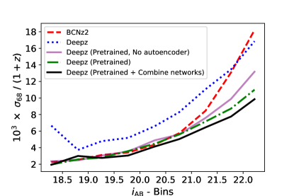
Figure 2: The $\sigma_{68}/(1+z)$ metric for 100% of the galaxies with secure redshifts in magnitude bins and for different codes. The dashed (red) line is the baseline performance and it corresponds to the BCNz2 results from Eriksen et al. (2019). The rest of the lines show the results for various DEEPz configurations.

Figure 2 shows the main photo-$z$ results, which uses the training procedure explained in §2. For quantifying the photo-$z$ performance, we define

$$\sigma_{68}\equiv 0.5\left(z_{\rm quant}^{84.1}-z_{\rm quant}^{15.9}\right)$$ (4)

which is half the difference between the 84.1 and 15.9 percentile. The $\sigma_{68}$ corresponds to the standard deviation for a Gaussian distribution, but is less sensitive to outliers. Throughout the paper we also use a strict outlier defined by

$$|z_{\rm p}-z_{\rm s}|\ /\ (1+z_{\rm s})>0.02$$ (5)

where $z_{\rm p}$ and $z_{\rm s}$ are the photometric and spectroscopic redshift, respectively. We label this outlier fraction ‘strict’, since it should not be confused with what is an outlier in a broad-band survey. In a broad-band survey the photo-$z$ scatter is much larger and the corresponding outlier definition (Eq. 5) is often 10 times more relaxed (Kuijken et al., 2015; Bilicki et al., 2018).

The dashed line (Fig. 2) shows the photo-$z$ scatter using the BCNz2 template fitting code as a function of differential $i$-band values. The dotted line shows the performance when training Deepz only on observed data. The photo-$z$ scatter is significantly larger than for BCNz2, except for the faintest magnitudes ($21.8<i_{\rm AB}$). Pre-training the network on simulations before training with data reduces the photo-$z$ scatter by  50% at the faint end. Not including an autoencoder, as discussed further in the next section (§4), degrades the performance at the faint end. Lastly, the solid line shows the result when training the networks 10 different times with multiple networks (see §2.4 and §5.2). These are the currently best Deepz results. In appendix D we have included a photo-$z$ versus spec-$z$ plot to highlight the outliers.

When pretraining with either the FSPS and template simulations (§3.2), we find a significant reduction in the photo-$z$ scatter. For the cases of no-pretraining, pretraining on template simulations and pretraining on the FSPS simulations, the $\sigma_{68}/(1+z)$ without quality cuts is 0.0095, 0.0077 and 0.0069, respectively. This indicates that a better SED modelling is more important than a correct colour space distribution for simulation used for pre-training. We have also tested generating the FSPS simulations fixing the gas ionisation fraction, which gave a slightly higher scatter. Other approaches to improve the simulations could lead to an even better performance.

3.4 Redshift intervals without spectroscopic galaxies

A fundamental limitation when training the PAUS photo-$z$ is the small training set. Deep neural networks are often trained with millions of training samples, e.g. in ImageNet (Deng et al., 2009). Transfer learning from simulation is one approach for reducing the required number of spectroscopic galaxies.

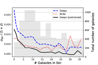
Figure 3: The effect of redshift ranges with a smaller number of galaxies. On the x-axis is the number of galaxies in bins of $\Delta z=0.001$. The dotted line shows the BCNz2 result, while the continues and dotted lines show the Deepz when pretraining or not on simulations. The shaded histogram displays the total number of galaxies for each value on the x-axis.

Figure 3 shows the photo-$z$ scatter as a function of the number of galaxies in the bin for bins of $\Delta z=0.001$. We want to understand how the density of spectroscopic redshifts affects the photo-z scatter. These bins are only used to illustrate the effect of the density and are not used when training the MDN. With the Deepz code, the photo-$z$ scatter is clearly higher in bins with only a few galaxies. A dotted line shows the BCNz2 result which is much less affected by the number of galaxies per bin, specially for very sparse bins. This shows that the number of galaxies in the bin is the underlying reason and not by bins with few galaxies indirectly select higher redshifts. Pretraining on simulations reduces the difference, but there is still a region with fewer galaxies where the template fitting works better. Lastly, appendix E details how to deal with low density regions for networks without a MDN.

In addition, we have tested using the mixup (Zhang et al., 2017) method of data augmentation. Normally data augmentation requires knowing which transformation can be applied without changing the meaning of the data. For example, when classifying images one might want to include rotations and slightly changing the brightness. Instead, the mixup method uses the linear combination of a random pair of inputs. Applying this technique to our data did not improve the photo-$z$ scatter.

4 Autoencoders

The network architecture includes an autoencoder (see §2.2). Section 4.1 explains with a single SED example how autoencoders can reduce the observational noise and extract features. Then in §4.2 we discuss application of the technique to our FSPS simulations and discusses the impact for redshift estimates.

4.1 Autoencoders

Figure 1 (top) of the Deepz network architecture shows the two autoencoder networks. The encoder network transforms its input into the latent or feature space. In our case, the input is 46 bands (40 NB, 6 BB) and the latent space has 10 variables, which is a reasonable number of parameters to describe a galaxy SED. A decoder network then attempts to reconstruct the input. One can train these networks with a loss function comparing the recovered values and the original input. Since the latent space is smaller than the input, the autoencoder is required to compress the information. The noise can not be compressed to fewer numbers and therefore gets removed.

Figure 4: Effect of the denoising network for one example galaxy. The simulation is generated from a single elliptical SED with arbitrary flux units and a uniform redshift distribution. The crosses and circles show the input and denoised narrow-band measurements, respectively. A solid line displays the noiseless flux of the SED.

To illustrate how the autoencoder works, we have generated a set of simple simulations. Using a single elliptical SED (Ell1_A_0) that was used both in the COSMOS2015 (Laigle et al., 2016) and the PAUS photo-$z$ papers (Eriksen et al., 2019), we estimate galaxy fluxes for a uniform redshift distribution. We added Gaussian noise with $\text{SNR}=10$ and 35 for the narrow and broad bands, respectively, which corresponds to the noise level for a bright PAUS galaxy. This simulation is then used to train an autoencoder. Figure 4 compares the input, true and noise reduced fluxes for a typical case. The recovered output has clearly reduced noise. The autoencoder achieves this by using the fact that galaxies in this simulation do not populate the full colour space, but a 2D sub-manifold described by the redshift and amplitude.

Note that an autoencoder can also be applied to broad bands alone, where the input dimension is typically smaller than the latent space. With the method above, the autoencoder would simply become the identity mapping. This can be solved by adding Gaussian noise to the input fluxes (Vincent et al., 2010).

4.2 Tests on FSPS simulations

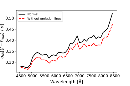
Figure 5: Top: The scatter ($\sigma_{68}$) of the difference of the difference of the denoised ($f$) and true fluxes ($f_{\rm True}$) relative the known errors of the input fluxes ($\sigma$). In the dashed line the bands with emission lines are removed. Bottom: The correlation matrix of the denoised flux between different narrow bands.

Figure 5 quantifies the impact of using an autoencoder on the FSPS simulations (§3.2). The top panel compares the error in the recovered fluxes with the input error, as a function of wavelength. A unity mapping would give a horizontal line at unity. When using the autoencoder, we find the flux errors decrease. For the blue bands the error is 30% of the expected value and it increases to 50% for the redder bands. For the broad bands, the ratio between the recovered and input error is 1.04, 0.72, 0.66, 0.61, 0.22 and 0.97 for the $uBVriz$ bands, respectively. A problem is that the autoencoder smooths the emission lines (see dashed line), which is a known artefact in autoencoders (Dosovitskiy & Brox, 2016). The recovered fluxes are good for training the redshift network, but should be used with caution for other scientific applications, e.g. estimating the mean flux.

The bottom panel (Fig. 5) shows the correlation between the different narrow bands. Here the broad bands are used to train the network, but not included in the figure for clarity. When using an autoencoder, the galaxy is transformed by the encoder into the latent space variables, which describe the galaxy. This transformation is affected by noise in the input and is also not perfect and this introduces an error on the latent variables. When reconstructing the fluxes with the decoder, this creates correlated noise between different bands. This can be understood from the latent space representing information related to galaxy type or dust properties. As can be seen, the correlation is strongest with nearby bands. Furthermore, there is a correlation between bands that are separated by 1500Å, resulting from confusing the $\text{O}_{\text{II}}$ and $\text{O}_{\text{III}}$ lines.

When training the redshift network (Fig. 1), we combine the information from the input fluxes and features produced by the autoencoder. Combining information processed in different ways together is a standard technique in deep learning (see e.g. Huang, Liu & Weinberger 2016). When training on the simulations, we combine the loss from both the autoencoder and the redshift estimation, while ignoring the autoencoder loss when fine-tuning on data. Fig. 2 includes a line where the auto-encoder is disabled by setting all features to zero. This shows the autoencoder has a significant impact on the photo-$z$ scatter for faint galaxies. We also expect the autoencoders to become more important when training the autoencoder with data in the wide fields (CFHTLenS W1 and W3) without spectra. We leave this for future work.

5 Adding information from individual exposures

We describe in §5.1 the motivation of including information from individual exposures when training the network, while §5.2 explores combining multiple networks to reduce the errors. Lastly, §5.3 studies the use of individual exposures at test time.

5.1 Incorporating individual exposures

Astronomical surveys perform repeated measurements over the same parts of the sky in systematic patterns. The purpose of making multiple observations is often to produce a combined measurement with reduced noise, allowing the observation of fainter objects. For example, the Dark Energy Survey (DES) (Hoyle et al., 2018) and the Kilo-Degree Survey (KIDS, Kuijken et al. 2019) have imaged each position $\sim 8$, $4-5$ times in each band, respectively. The Rubin Observatory Legacy Survey of Space and Time (LSST) will measure each location several hundred times (LSST Science Collaboration et al., 2009). In PAUS, the COSMOS field is nominally imaged at least 5 times in each narrow band.

For estimating the redshifts, the individual measurements are typically first combined into coadded fluxes. A standard choice is to combine the individual measurements by an inverse variance weighting, which is statistically optimal for a combination of independent Gaussian measurements. However, this combination is not optimal if there are photometric outliers. These outliers can arise from multiple sources including scattered light (Cabayol et al., 2019), electronic cross-talk between the charge-coupled devices (CCDs) or data reduction issues in the calibration or photometry.

Removing problematic measurements is difficult. The PAU data management (PAUdm) code flags many of the problematic outliers based on image diagnostics. Outliers are however still present in the PAUS data. The PAUS observations are often noisy (${\rm SNR}<1$) and for many (galaxy, band) combinations, we only have 3 exposures after flagging measurements, making the detection of outliers for a single band hard. Some outliers, like those resulting from negative cross-talk, are clearly visible, since the flux is much lower than nearby bands. However, positive flux outliers are harder to flag and are problematic since they can be confused with emission lines, leading to photo-$z$ outliers.

Instead of manually removing measurements, we want the photo-$z$ code to select itself the correct measurements by working directly with the individual exposures. The most obvious approach would be to directly input the individual exposures to the network. However, multiple problems arise when applying the technique to observational data. For example, PAUS has a minimum of 5 exposures in the COSMOS field, however, many of the observations are removed since they contain bad data. Also, there are regions with more than 5 exposures. This means the input to the photo-$z$ code would not be a dense array with all values present.

Furthermore, inputting all measurements individually drastically increases the network size. In addition to at least increasing the network with 5 times the inputs (number of exposures), one should also inform the network which measurements are present. If specifying a mask, this would lead to another doubling of the input. Also, the ordering of individual fluxes is not unique. Appendix F details how this problem can partially be overcome by permuting the order of the individual flux measurements when training. This approach does not solve the issue to the required accuracy.

An alternative approach builds on the technique of data augmentation. When training neural networks, it is common to perturb the input to produce a slightly different input. For example, one might crop, flip or adjust the colours of an image. This produces images humans essentially see as unchanged, but appear different to the network. Adding these permutations often ends up improving the performance and is standard for many applications (Perez & Wang, 2017).

The approach suggested in this paper is training the network with randomised coadds, constructed on the fly with a randomised selection of individual exposures. Each time when training the network with a set of galaxies, the individual exposures are chosen to be included with a probability $\alpha$. Since the coadded fluxes are constructed for each epoch, it means each galaxy will look different to the network at each epoch. We have tested two methods to handle galaxies not having measurements in all bands after the random selection. In one, the galaxy is removed for a specific epoch when the randomisation leads to not having measurements in all bands and the second modified the sampling method to ensure at least one measurement is present in each band. The construction of randomised coadds can be computed simultaneously on a GPU without significant computational overhead.

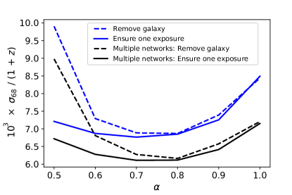
Figure 6: The $\sigma_{68}/(1+z)$ when varying the value of the probability of including an exposure in the coadd when training ($\alpha$). A factor of $\alpha=1$ corresponds to no randomness. Blue lines use a single network, while black lines combine multiple networks. For the dashed lines a galaxy is removed when the randomness leads to a galaxy not having measurement in all bands. Continuous lines use a randomisation procedure which is required to keep at least on measurement per band.

Figure 6 shows the photo-$z$ scatter for different probabilities of using the individual measurements ($\alpha$). Including this randomness when training significantly reduces the photo-$z$ scatter. When predicting with a single network, the photo-$z$ error decreases by 20% compared with no randomisation. The dashed lines show the result when one removes galaxies which do not have measurements in all 40 bands after applying the random exposure removal. Note that which galaxies are removed depends on the epoch, since the networks see each galaxy multiple times (appendix C). Below about $\alpha=0.7$, the networks performance degrades, which follows from many galaxies not being used in the training if not ensuring one exposure being present. By default results in this paper use $\alpha=0.8$. The result for the ‘Multiple networks’ will be discussed in §5.2.

Training a neural network means learning a mapping between the observed colours and the redshifts. In this process, the network also needs to discover which features are real or simply due to bad photometry. The randomised construction of the coadds when training leads to the network seeing the same galaxy with and without problematic measurements. This makes it easier to learn which features are properties of the galaxies, like the emission lines. This method is expected to be less effective in the limit of an infinite training sample. However, the randomisation makes an important difference for a limited training set with outlier measurements.

5.2 Combining predictions from multiple networks

The photometric redshift results discussed until now have used a 80-20 split between the training and test sample (see §2.4).

One could attempt to change the splitting ratio (e.g. 90-10) to increase the number of galaxies used for training. In the extreme limit one would have one network per galaxy, which would be prohibitively computationally expensive. Instead we focus on combining multiple networks and have defined ten (random) ways of splitting the catalogue into a training and a test sample. With this approach, one can train and combine the PDFs for multiple networks for each galaxy in the training set. Note, the estimated photo-$z$ always use networks which have not been trained with the same galaxy.

Figure 2, which compares the effect from different ideas, includes a line showing the photo-$z$ predictions using multiple networks. The photo-$z$ results shown correspond to training with ten different 80-20 splits and then averaging the resulting $p(z)$ distributions. This means training the networks in total 50 times. Combining the networks leads to about 10 percent lower photo-$z$ scatter for the faintest galaxies in the sample ($i_{\rm AB}=22.5$). We also tested generating the photo-$z$ using 100 different splits. The benefit of multiple networks saturated with fewer than 10 splits, which we use by default in the Deepz code.

In Figure 6 we also study the effect of combining multiple networks when randomly creating coadds. The two blue lines corresponding to a single network. Two black lines show the performance combining multiple networks. The photo-$z$ scatter for the two methods follows a similar trend. This result shows that combining multiple networks, rather than being redundant, is an improvement on top of the coadd randomization.

5.3 Test-time augmentation

In the previous subsection we applied data augmentation when training the network. Data augmentation can also be used when inferring the redshift, often named test-time augmentation and can be applied in addition to the training augmentation discussed in the previous subsection.

Training a neural network is often computationally expensive, although for our case, the training is faster than the BCNz2 template fitting method. Predicting the redshift is very fast with neural networks. This allows studying how the photo-$z$ is affected by changes in the photometry. In this section, we have tested systematically removing individual fluxes, constructed the coadded fluxes and estimated the corresponding photometric redshifts.

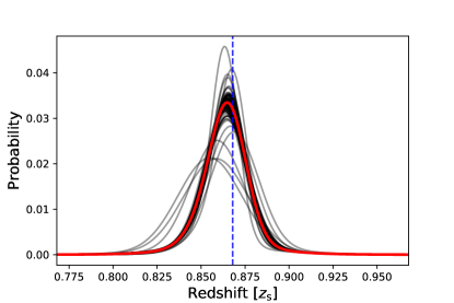
Figure 7: Test time augmentation, removing individual flux measurements for a single galaxy. The vertical line indicates the redshift, while the solid red line gives the $p(z)$ using the full coadd. The thin lines show the $p(z)$ estimated without individual flux measurements.

Figure 7 shows the effect of dropping different exposures for an example galaxy. Here the vertical line marks the spectroscopic (true) redshift, the thin lines show the $p(z)$ for different removed exposures and the solid red line shows the $p(z)$ estimated from the coadds. In most cases, the $p(z)$ distributions peak at a redshift that is slightly shifted from the spectroscopic redshift. When dropping one of the exposures, the $p(z)$ prediction peaks around the spectroscopic redshift. In other cases, dropping a single exposure leads to the $p(z)$ moving in the wrong direction and therefore produces an outlier. From this experiment, we conclude that systematically estimating the photo-$z$ by dropping individual measurements is not a viable strategy.

6 Validating the redshift distribution

In this section we validate whether the redshift probability distributions accurately represent the uncertainties (§6.1). We also introduce redshift quality cuts (§6.2) to select subsamples with better redshift determination.

6.1 Validating the redshift distributions

The Deepz code does not only predict a point estimate, but also the redshift probability density. Knowing the redshift distribution for each object is useful for various applications, like e.g. weak gravitational lensing measurements. For this reason, it is important that the PDFs actually represent the redshift uncertainty, not simply peaking around the correct redshift.

A common approach for testing the quality of the probability distribution is the probability integral transform (PIT, Dawid 1984; Gneiting et al. 2005; Bordoloi, Lilly & Amara 2010)

$$\text{PIT}=\int_{0}^{zs}dz^{\prime}p(z^{\prime})$$ (6)

where $p(z)$ is the probability distribution and the integration is from zero to the spectroscopic redshift ($z_{s}$). If the probability distribution estimate actually represents the underlying distribution, the distribution of PIT values would be uniform.

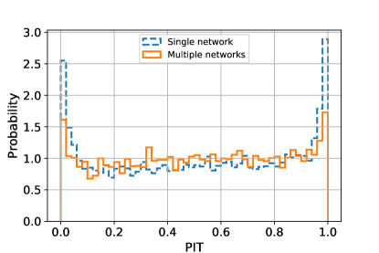
Figure 8: Testing the $p(z)$ distributions using the PIT distribution. The solid line shows the result when combining multiple networks, while the dashed line shows the result for a single network.

Figure 8 shows the PIT distribution for Deepz of the test set. The dashed line shows the the result for a single network, while the solid line shows the result for multiple networks. The distributions are close to uniform, except for low and high PIT values. These peaks correspond to photo-$z$ outliers which are not reflected in the PDFs predicted by the network. The main contribution behind the drop when combining multiple network is the combined networks reduce the outlier rate, making the $p(z)$ simpler to estimate.

The uniformity of the PIT diagram should not be taken for granted. In addition to problems with outliers, many redshift codes have a problem, underpredicting the width of the redshift PDFs (Schmidt, Weeds & Higgins, 2020). In early versions of this work, we predicted the probability distribution using a classifier, binning the galaxies in different bins. The resulting PIT histograms were not sufficiently flat. In Guo et al. (2017) the authors claim that the classical neural networks have PDFs that are relatively well calibrated, but this is no longer the case when dealing with modern architectures. These include many components, like the batch normalisation and weight decay, which leads to reported probabilities to not accurately represent the true distribution. Using a mixture density network (§2.3) provides better probability distributions for our application.

6.2 Quality cuts

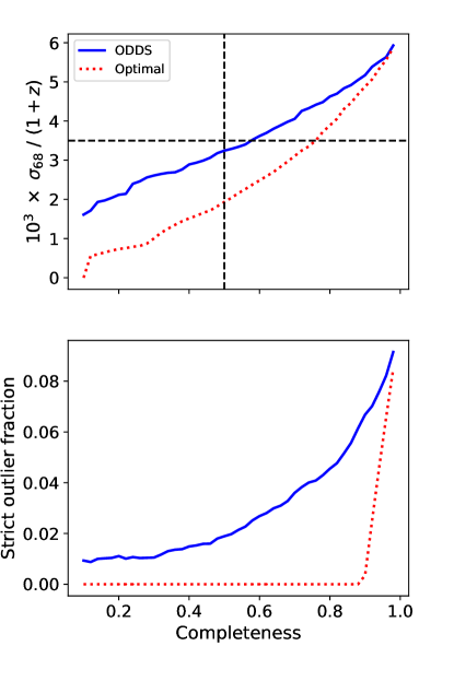
Figure 9: The effect of introducing photo-$z$ quality cuts for the secure redshift sample to $i_{\rm AB}<22.5$. The top and bottom panels show the photo-$z$ scatter and outlier rate, respectively. Continuous lines cuts based on the ODDS parameter, defined from the probability distribution. The optimal lines cut based on the spectroscopic redshifts to demonstrate the (idealistic) lower limit of a quality cuts. The horizontal line in the top panel corresponds to PAUS photo-z target for a selected 50% of the sample.

This subsection studies introducing redshift quality cuts for the Deepz code, but one should be aware of the potential side effects of these cuts. For different science applications, one might want to select a subset of galaxies with higher photometric redshift precision, e.g. to cross-correlate galaxy counts with other samples to estimate the photo-$z$ scatter between redshift bins. A common problem with cutting on photometric redshift quality is unintentionally introducing clustering, since the quality might be tracing spatial patterns like observing conditions (Ross et al., 2011; Martí et al., 2014). In Eriksen et al. (2019) we reported on visible spatial patterns in the quality of the BCNz2 template fitting. The ODDS quality parameter introduced in BPZ (Benítez, 2000) is defined by

$$\text{ODDS}\equiv\int_{z_{0}-\Delta z/2}^{z_{0}+\Delta z/2}dz\,p(z)$$ (7)

where $p(z)$ is the probability distribution, $z_{0}$ its mode and $\Delta z=0.003$ being the fixed interval around the most likely redshift (mode of the distribution).

Figure 9 shows the photo-$z$ scatter (top) and strict outlier rate defined in Eq. 5 (bottom) as a function of the completeness, which is the fraction of galaxies kept after the cut. Introducing a quality cut based on ODDS gives a significantly better photo-$z$ scatter and outlier rate. The PAUS Deepz redshifts for 50% now clearly surpass the target performance of $\sigma_{68}=0.0035(1+z)$ to $i_{\rm AB}=22.5$. It is likely that the scatter is higher, since galaxy types lacking spectral coverage will probably have a lower quality photo-$z$ estimate. The optimal lines select by $|z_{p}-z_{s}|$ using the spectroscopic information and indicate there might be further room for improving the quality cut.

In Eriksen et al. (2019) we tested the performance for a set of quality parameters. There we also used the pz_width quality parameter that measures the distance between the 1 and 99 percentile of the PDFs. For Deepz, we find that this quality parameter performs worse. By default, the BCNz2 results were reported using an adjusted version of the Qz parameter (Brammer, van Dokkum & Coppi, 2008), which is a multiplicative combination of the ODDS, the pz_width parameter and the $\chi^{2}$ of the fit. Unlike a template fitting code, the MDN network of Deepz directly estimates the $p(z)$ with normalisation. Therefore we cannot use the same quality cut.

In §5 we introduced a technique of randomly generating the coadds when training the network. We have tested generating the photo-$z$ for these different coadds based on 80% of the exposures and then estimating the variance between the different photo-$z$ estimates. Our initial expectation, was that smaller photo-$z$ variations would indicate a more secure photometric redshift determination. Actually, often the opposite is true. When there are very small variations when removing exposures, a subset of the exposures tends to drive the photo-$z$ solution. Cutting to keep galaxies with a higher variability in the predictions tends to perform better. However, this is a weaker quality cut than e.g. the ODDS.

7 Conclusions

In this paper we introduced a new deep learning photo-$z$ code, Deepz. We uses the Physics of the Accelerating Universe Survey (PAUS), which has 40 narrow bands (Padilla et al., 2019), as a test case. Previous work showed how PAUS can achieve the target photo-$z$ precision using a template based fitting code (Eriksen et al., 2019). This in itself is a non-trivial result, since previous attempts to apply ANNz and DNF (De Vicente, Sánchez & Sevilla-Noarbe, 2016) to PAUS simulations were unsuccessful. The standard ANNz essentially ignored the narrow bands because of their lower signal to noise ratio. Also, the lack of sufficient training data resulted in the codes being unable to reach the target photo-$z$ precision. In this paper we introduced a machine learning approach to overcome this obstacle and obtained state-of-the-art PAUS redshift precision.

The network was trained using flux ratios from the 40 PAUS narrow bands, combined with the CFHTLenS $u$-band and $BVriz$ bands from the Subaru telescope in the COSMOS field. The network inputs are the 46 fluxes, normalised to the $i$-band. To train the network, we used the zCOSMOS DR3 catalogue, limited to secure redshifts and simulations. The network was implemented using the PyTorch (Paszke et al., 2017) library, a widely used framework in the deep learning research community. Our architecture consisted of three different networks, an autoencoder to extract information about the galaxy and a network to predict the redshift. The network estimated the full PDF using a mixture density network (MDN) (Bishop, 1994) and the final distribution is the mean redshift PDF from an ensemble of 10 different networks.

The application of the machine learning approach based on only observed data as a training shows worse performance than the template method (BCNz2). However, transfer learning from simulations improves the photo-$z$ precision, especially for faint magnitudes. Combining the predictions from multiple networks further improved the scatter. For $i_{\rm AB}=22.5$ and without quality cuts, we found $\sigma_{68}$ to be 50% lower with Deepz compared to BCNz2, while the strict outlier fraction ($|z_{p}-z_{s}|>0.02$) reduces from 17 to 10 percent.

This paper tested transfer learning using two different simulations. The simulation based on the FSPS code performed significantly better than a template based simulation, indicating the SED modelling being important. For both simulations, the photo-$z$ continued improving until reaching the maximum number of observed redshifts available. This indicated there is further room to improve the PAUS photo-$z$ precision. Furthermore, the redshift performance was shown to depend on the number of galaxies for different redshifts (Fig. 3). For high densities, the network is clearly superior, but the template fitting code performs better at redshifts with very few spectra. Pretraining with simulations eases the situation, but not fully and this is an area of ongoing investigation.

Galaxy surveys typically take multiple exposures in each band, which are then combined into a single statistically optimal measurement (coadd). Since the coadd combines multiple measurements, it can be sensitive to outliers. We tested methods to include information from individual flux measurements. Instead of modifying the network architecture, we trained the network using coadds generated on the fly from a random selection of individual exposures. This approach resulted in a 20% reduction in the photo-$z$ scatter (Fig. 6). Combining multiple networks led to an additional 10% improvement.

The network architecture also included an autoencoder, which is useful to extract features and reducing noise. An autoencoder consists of an encoder network compressing the input to a set of ten features, while the decoder network attempts to reconstruct the original input. Optimising the difference between the input and reconstructed values is known to reduce the noise. We found a 50-70% reduction in the errors, with the largest effect for the blue bands. Furthermore, we showed how the autoencoder can lead to correlated errors between bands. Including features extracted from the autoencoder leads to a moderate reduction in the photo-$z$ scatter. The autoencoder is expected to be more important for the wider fields, since this type of network can be trained without spectroscopic redshifts.

The Deepz code estimates redshift probability distributions (PDF), which are not provided by many machine learning codes. The probability distributions were estimated using a mixture density network (MDN). We validated the PDFs with the probability integral transform (PIT) and found the $p(z)$ distributions represent the true underlying probability distributions, with the exception of some outliers. The PDF, when combining the networks, performed even better, mostly due to having fewer outliers to model. Lastly, we tested quality cuts based on the PDFs and found the Deepz photo-$z$ to exceed the PAUS target performance when selecting the 50% best galaxies based on a quality cut.

The uniqueness of PAUS is the wide fields, where PAUS have observed a total of 47 sq. deg. with 11, 14 and 20 sq.deg. in the CFHTls W1, W2 and W3 fields, respectively. The SNR of PAUS in the wide fields is comparable to the COSMOS fields, although with fewer exposures per galaxy and band ($\sim 5$ exposures in COSMOS and 3 in the wide fields). The differences between the fields are the broad bands (CFHT Megacam instead of Subaru), the galaxy parameter (e.g. size, ellipticity) used for the forced photometry from a different parent catalogue and the spectroscopic training set. All fields are calibrated relative to the SDSS stars. We are currently working on validating and homogenising the data reduction for the different fields. Potentially the Deepz network can be trained on COSMOS and use transfer learning to adapt to differences between the fields. Also, the extrapolation beyond the spectroscopic subset is as always uncertain and should be verified using e.g. galaxy cross-correlations (Schneider et al., 2006; Newman, 2008). This is work in progress and beyond the current paper.

In this paper we introduced an efficient deep learning technique for high precision redshift estimation. The network was tested with PAUS, but many ideas are not necessarily restricted to narrow-band surveys. Pre-training with simulations holds the promise of combining theoretical knowledge and empirical data from spectroscopic surveys. Also, the technique of randomly constructing coadds should be applicable to large weak lensing surveys, including LSST and Euclid.

Data availability

The PAUS observations are currently not publically available, while the deepz code is available upon request.

Appendix A BCNz2 photometric redshift code

In Eriksen et al. (2019) we described the BCNz2 photometric redshift code. This code was developed to reach good photometric redshift precision with PAUS. The code models the galaxy SED as a linear combination of templates

$$f^{\mathrm{Model}}_{i}[z,{\bm{\alpha}}]\equiv\sum_{j=1}^{n}f^{j}_{i}(z){\bm{\alpha}}_{j},$$ (8)

where $f^{i}_{j}$ is the model flux for template $j$ in band $i$. The ${\bm{\alpha}}$ vector includes the weights of the different SEDs. The estimated redshift probability distribution is given by

$$p(z) \propto\exp\left(-0.5\min_{{\bm{\alpha}}\geq 0}\chi^{2}[z,{\bm{\alpha}}]\right)$$ (9)

with the $\chi^{2}$ expression to minimised being defined by

$$\chi^{2}[z,{\bm{\alpha}}]\equiv\sum_{i,NB}\left(\frac{\tilde{f_{i}}-l_{i}kf^{\mathrm{Model}}_{i}}{\sigma_{i}}\right)^{2}+\sum_{i,BB}\left(\frac{\tilde{f_{i}}-l_{i}f^{\mathrm{Model}}_{i}}{\sigma_{i}}\right)^{2}.$$ (11)

Here the minimisation algorithm (Sha et al., 2007) ensures positive amplitudes (${\bm{\alpha}}$). The factors $l_{i}$ are global zero-points per band (i), while $k$ is a free scaling between narrow and broad bands per galaxy. These factors were introduced to reduce the sensitivity to calibration problems and issues in the PAUS photometry.

The zero-points $l_{i}$ were calibrated by comparing the observed flux and the best fit model when running the photo-$z$ code at the spectroscopic redshift. This additional zero-point calibration is commonly used and can account for residuals in the instrumental calibration. However, this method can effectively adjust the templates, introducing an erroneous zero-point calibration for a subset of galaxies. We are currently in the process of building on the work in Eriksen et al. (2019) and have studied the impact of the additional zero-point calibration (Alarcon in prep.). The Deepz code has the advantage of not requiring this calibration step, since it is a machine learning method which directly maps observed quantities to the redshift.

Appendix B Effect of photometric outliers

Estimating the photometric redshift with a template fitting code relies on an analytical likelihood function specifying the data probability given a model. This is the case for e.g. LePhare (Arnouts & Ilbert, 2011; Ilbert et al., 2006) and BPZ (Benítez, 2000). In the likelihood and fitting, the input data are often assumed to have Gaussian and known errors. Unfortunately, observed data also includes outliers, which are not reflected in the likelihood. For PAUS, there are problems in the calibration, the photometry, cross-talk between CCDs and other issues. While removing outliers is a target of the PAU data reduction, there will always be some errors remaining.

Ideally the photo-$z$ code should be insensitive to outliers in the input data. Template fitting codes can in theory be extended to model the outliers by modelling the flux errors as a linear combination of the standard error and a wider Gaussian describing the outliers. In practice the idea has multiple complications. Many photo-$z$ codes rely on the specific functional form of the likelihood ($\chi^{2}$) expression. The BCNz2 code use a non-negative minimisation algorithm working with quadratic functions, which makes it hard to incorporate many ideas. Furthermore, modelling the outliers would require setting the outlier rate, which should potentially depend on the SNR of the input data.

Machine learning codes are often more robust towards photometric outliers. To test this idea, we have generated a simple set of galaxy mocks. In this test, we generate a set of 10000 elliptical galaxies. These use 8 elliptical galaxies SEDs without extinction or emission lines, corresponding to the first template set in BCNz2 (run 1). We add Gaussian noise with SNR of 10 and 35 in the narrow and broad bands, respectively. The outliers are generated by adding an additional flux in the $u$-band to all galaxies in the test set (see Fig. 10).

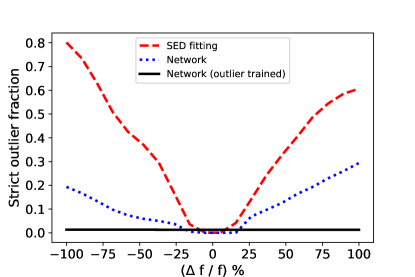
Figure 10: The effect of outliers in the photometry on the strict photo-$z$ outlier fraction. On the x-axis is the percentage $u$-band flux added to all galaxies in the test set. The result is shown for a SED fitting, a neural network and a neural net trained with simulations including outliers.

Figure 10 demonstrates the impact on photometric outliers on classical template fitting and machine learning approaches. The figure shows the strict outlier fraction (Eq. 5) as a function of an additional flux fraction applied to the $u$-band for all galaxies in the test sample. For the ‘SED fitting’ line, we fit the galaxies to elliptical templates with a minimum $\chi^{2}$ approach. This is an optimistic estimate since we perfectly know the SEDs and have not included other galaxy types. For the network we use the architecture and training procedure outlined in §2.

The template fitting is strongly sensitive to the outliers, while the neural network is less sensitive. An approach to further reduce the impact of photometry outliers is adding outliers to the training data. In this way the network learns to not blindly trust features since they could also be photometric outliers. We have tested adding 10% outliers uniformly distributed over the different bands and with varying amplitudes which is shown in Fig. 10. Note that we are not informing the network which galaxies have problematic photometry. The network trained with photometry outliers becomes remarkable insensitive to these, as indicated by the essentially flat solid line.

Appendix C Deep learning basics

Deep learning and artificial intelligence (AI) has become an important trend over the last years. The usage of graphical processor units (GPUs) with massive parallelization has enabled training large models with large amounts of data. Furthermore, this renewed interest has introduced a new set of different techniques like generative adversarial networks (GANs) (Goodfellow et al., 2014), reinforcement learning (Kaelbling, Littman & Moore, 1996), new network architectures (He et al., 2015) and the attention mechanism (Vaswani et al., 2017). While this paper only uses a small set of techniques, it benefits from the overall activity in the field. This includes the access to well documented, open-source libraries for neural networks, like PyTorch (Paszke et al., 2017) and Tensorflow (Abadi et al., 2015).

Neural networks are a machine learning technique, which has a long history with early implementations in the 1950s (Rosenblatt, 1958). The usage of neural networks was in periods overpromising with successive periods of being out of fashion. Groundbreaking results on image classifications achieved by training a larger neural network with many images led to renewed interest in the field (Krizhevsky, Sutskever & Hinton, 2012).

Deep learning is effectively a neural network with many layers. The network consists of multiple layers or transformations of the data. While the performance with a few layers tends to flatten when increasing the amount of training data, the performance of deep networks tends to increase with more data. This training is often computationally expensive but can use graphics processing units (GPUs), which supports massive multiprocessing.

There are multiple types of neural networks, including convolutional neural networks (CNNs) and recursive neural networks. In this paper we use a linear neural network and will briefly explain these. The network consists of a series of transformations to the data, or layers, which are sequentially applied to the data. A linear layer is the transformation

$$\rm{linear(}\mathbf{x}\rm{)}\equiv\mathbf{A}\mathbf{x}+\mathbf{b}$$ (12)

where $\mathbf{x}$ is the input data, while the matrix $\mathbf{A}$ and vector $\mathbf{b}$ are parameters of the the neural network. These network parameters will be initiated randomly and trained using the data.

For the network to learn a non-linear mapping from the input, it also need to include a non-linear transformation or activation function. A common choice is the ReLU activation function, which is defined by

$$\rm{ReLU(}\mathbf{x}\rm{)}\equiv\left\{\begin{array}[]{@{}lr@{}}0,&\text{for }\mathbf{x}\leq 0\\ \mathbf{x},&\text{for }0\leq\mathbf{x}\end{array}\right.$$ (13)

where the operation is performed element-wise. Explained with words, the ReLU activation sets negative entries to zero.

In addition, this work uses Batch Normalisation (Ioffe & Szegedy, 2015). The batch normalisation is a layer standardising the input to the layer to have mean zero and unit variance. This transformation is known to make neural networks faster to train, more robust and achieve better performance. When constructing the network, we include a dropout layer, randomly dropping a few percentages of the values. This technique is often used to hinder over-fitting, the effect of the network fitting well to the training data, but not generalising to data for which the network is not trained.

For supervised training the network predictions are compared with a known answer (or labels). One then constructs a loss, which measures how wrong the network prediction is. In our case the main contribution to the loss is given by the negative logarithm of the estimated probability at the spectroscopic redshifts (Eq. 2). The training of the network is done using batched, which is a subset of galaxies jointly used to estimate the batch loss and update the network. Dividing in batches is done to train the network faster. When having trained with all data once, we say the network has been trained for an epoch.

Updating the network parameters use the Adam optimiser. When training we include weight-decay (Krogh & Hertz, 1992), which is a technique which adds an additional loss that limits too high parameters. In practice, this is implemented as a decay term when updating the weights. Furthermore, how fast the network is updated is controlled by the learning rate. A high learning rate reduces the training time, but risk the network being stuck in a sub-optimal solution.

Appendix D Photo-z scatter

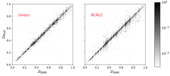
Figure 11: Density plot comparing Deepz (left) and BCNz2 (right) redshift predictions to secure zCOSMOS DR3 spectroscopic redshifts. The colour scale is logarithmic to view the outliers.

Figure 11 shows a 2D histogram plot for Deepz and BCNz2. The colour scale is logarithmic colour scale to better visualise the outliers. Otherwise most PAUS galaxies of the galaxies were forming a narrow diagonal line.

Appendix E Label smoothing

While photo-$z$ estimation is fundamentally a regression problem, it is often implemented using a classifier (e.g. Bonnett 2015), with classes corresponding to thin redshift bins. For a broad-band survey, one can typically use bins of $\Delta z=0.015$. However, for PAUS we need to use $\Delta z=0.001$ wide bins to also capture galaxies with excellent ($\sigma_{68}=0.001(1+z))$ redshift precision at the bright end. This would require 15 times more bins. As a result, the size and number of weights in the last linear layer, which has a large fraction of the weights, increases dramatically. The last layer would have approximately 15 times more parameters for a narrow-band photo-$z$ compared to the broad-band equivalent.

We have tried implementing a photo-$z$ classifier with different approaches to account for different numbers of galaxies in each class. In Buda, Maki & Mazurowski (2018) the authors review the state of solutions to class imbalance in the literature. They found that oversampling, i.e. selecting samples more often from less probable classes, tends to give the best results.

The classifier approach ignores the information from nearby redshifts. For a example, there is no concept of nearby classes when predicting the animal type with a traditional classifier. With PAUS data, the fundamental limitation is redshift bins without spectroscopic galaxies. When decreasing the bin size, there will be bins without galaxies. No matter the weighting scheme, these bins will remain empty. Not having a concept of nearby redshift is an artefact of framing a regression problem as a classification.

One approach to avoid empty redshift bins is label smoothing (Simard et al., 2012). Instead of assigning a galaxy to a single redshift bin/class, the redshift is randomly scattered to one of the nearby redshift bins/classes. Applying this technique when training significantly reduces the photo-$z$ scatter. Tests with applying different scatter values, resulted in a different optimal scatter for bright and faint galaxies, with the photo-$z$ scatter reduced most significant for large redshift scatter. Instead of using a fixed value or hard-coded relation, we have developed a method to estimate the required smoothing from the PDF. In each step, we predict the $\sigma_{68}$ of the estimated redshift PDF. This can be done fast on the GPU with a cumulative sum. The redshift scatter is then introduced as a Gaussian smoothing with 15% of the $p(z)$ width. While this leads to a significant reduction in the photo-$z$ scatter, the resulting photo-$z$ scatter is comparable with an MDN without the smoothing step. In addition, the PDFs produced by the MDNs were better giving the true distribution (§6.1) and give better quality cuts. This paper therefore uses the MDN for estimating the probability distributions.

Appendix F Network using individual exposures

In this paper the default method of including information from individual exposures is by data augmentations when training the network. This is done by constructing coadds during the training from randomised subsets of exposures (see §5). Here we briefly report on challenges encountered when constructing a network architecture to directly estimate the redshift from individual exposures.

A problem for creating a network using individual exposures is the irregularity of the data. While galaxy surveys strive to obtain uniform coverage over the field, the number of exposures will always depend on the sky-position. The standard types of neural network work best with regular data, for example 2D images and 1D series of observations. This would require inputting the data with all bands having the same number of observations. With observational data, this would use the lowest number for all galaxies, which would lead to dropping an unacceptable fraction of observations.

Alternatively, one can construct a larger data structure and set the missing observations to a special value. Also, the position of the missing values can be given to the network as an additional mask. These approaches work partly for our data, but they do not reach a sufficiently low photo-$z$ scatter. This appendix uses a simplified simulation to explain potential pitfalls with this approach. For testing the effect of individual exposures, we use the standard network with one modification. When inputting the individual exposures, the first layer has the dimension needed for working with a flattened array of the individual exposures. For simplicity, we did not include the broad-band measurements.

Figure 12: The scatter between the photo-$z$ when estimating the redshift with different exposure orders for different approaches for training the network (see text). The vertical lines show the $\sigma_{68}$ for a single exposure order.

One needs to define an order of the exposures when inputting the individual exposures as a matrix (tensor). Given the exposures are a set, the network will need to learn that these measurements have the same meaning. One approach is using training augmentation, randomly mixing the order of the individual fluxes. This allows the network to learn more easily the meaning of the individual exposures from the limited spectroscopic dataset.

Furthermore, the order also makes a difference when estimating the redshifts. Figure 12 shows scatter between photo-$z$ predicted with different exposures order for different randomisation strategies when training the network. Here only 30% of all individual fluxes are present and the input is given as a dense matrix without inputting an additional mask. After training the network, we test predicting the photo-$z$ for different orders of the exposure. The x-axis shows the photo-$z$ scatter between specifying the individual fluxes in a different order. This is not the normal photo-$z$ error, but an additional error coming only from the ordering of the individual fluxes.

The ‘No augmentation’ line is trained without any data augmentation, leading to a large photo-$z$ scatter. Reordering the measurements during training can be computational expensive. One simple approach is to only switch the order of the input fluxes in each batch. This still produces $5!=120$ orders of the input per band for five exposures. As shown in the ‘Same shuffle’ line, this decreases the spread among the predictions. Finally, we have tested fully permuting the different inputs when training. For 40 bands, this implies ${40}^{120}$ different configurations of which we will only sample a small subset. The ‘Independent shuffle’ line shows the result when fully randomly selecting the exposure order for each galaxy and band, each time the network is trained (epoch). This further improves the scatter, but it’s still too large.

References

- Abadi et al. (2015) Abadi M. et al., 2015, TensorFlow: Large-scale machine learning on heterogeneous systems. Software available from tensorflow.org
- Arnouts & Ilbert (2011) Arnouts S., Ilbert O., 2011, LePHARE: Photometric Analysis for Redshift Estimate
- Bartelmann & Schneider (2001) Bartelmann M., Schneider P., 2001, Phys. Rep., 340, 291
- Baum (1962) Baum W. A., 1962, in IAU Symposium, Vol. 15, Problems of Extra-Galactic Research, McVittie G. C., ed., p. 390
- Benítez (2000) Benítez N., 2000, ApJ, 536, 571
- Bilicki et al. (2018) Bilicki M. et al., 2018, A&A, 616, A69
- Bishop (1994) Bishop C. M., 1994, Mixture density networks. Tech. rep.
- Blanton et al. (2003) Blanton M. R. et al., 2003, ApJ, 592, 819
- Blanton et al. (2005) Blanton M. R. et al., 2005, AJ, 129, 2562
- Bonnett (2015) Bonnett C., 2015, MNRAS, 449, 1043
- Bordoloi, Lilly & Amara (2010) Bordoloi R., Lilly S. J., Amara A., 2010, MNRAS, 406, 881
- Brammer, van Dokkum & Coppi (2008) Brammer G. B., van Dokkum P. G., Coppi P., 2008, ApJ, 686, 1503
- Brown et al. (2018) Brown A. G. A. et al., 2018, Astronomy & Astrophysics, 616, A1
- Buda, Maki & Mazurowski (2018) Buda M., Maki A., Mazurowski M. A., 2018, Neural Networks, 106, 249
- Byler et al. (2017) Byler N., Dalcanton J. J., Conroy C., Johnson B. D., 2017, ApJ, 840, 44
- Cabayol et al. (2019) Cabayol L. et al., 2019, MNRAS, 483, 529
- Cabayol-Garcia et al. (2019) Cabayol-Garcia L. et al., 2019, MNRAS, 2934
- Calzetti et al. (2000) Calzetti D., Armus L., Bohlin R. C., Kinney A. L., Koornneef J., Storchi-Bergmann T., 2000, ApJ, 533, 682
- Chabrier (2003) Chabrier G., 2003, PASP, 115, 763
- Collister & Lahav (2004) Collister A., Lahav O., 2004, Publications of the Astronomical Society of the Pacific, 116, 345–351
- Conroy & Gunn (2010) Conroy C., Gunn J. E., 2010, ApJ, 712, 833
- Conroy, Gunn & White (2009) Conroy C., Gunn J. E., White M., 2009, ApJ, 699, 486
- Dawid (1984) Dawid A. P., 1984, Journal of the Royal Statistical Society. Series A (General), 147, 278
- De Vicente, Sánchez & Sevilla-Noarbe (2016) De Vicente J., Sánchez E., Sevilla-Noarbe I., 2016, MNRAS, 459, 3078
- Deng et al. (2009) Deng J., Dong W., Socher R., Li L.-J., Li K., Fei-Fei L., 2009, in CVPR09
- Dosovitskiy & Brox (2016) Dosovitskiy A., Brox T., 2016, preprint (arXiv:1602.02644)
- Eriksen et al. (2019) Eriksen M. et al., 2019, MNRAS, 484, 4200
- Eriksen & Gaztañaga (2015) Eriksen M., Gaztañaga E., 2015, MNRAS, 452, 2168
- Ferland et al. (2013) Ferland G. J. et al., 2013, Rev. Mexicana Astron. Astrofis., 49, 137
- Gaztañaga et al. (2012) Gaztañaga E., Eriksen M., Crocce M., Castander F. J., Fosalba P., Marti P., Miquel R., Cabré A., 2012, MNRAS, 422, 2904
- Gerdes et al. (2010) Gerdes D. W., Sypniewski A. J., McKay T. A., Hao J., Weis M. R., Wechsler R. H., Busha M. T., 2010, ApJ, 715, 823
- Gneiting et al. (2005) Gneiting T., Raftery A. E., Westveld A. H., Goldman T., 2005, Monthly Weather Review, 133, 1098
- Goodfellow et al. (2014) Goodfellow I. J., Pouget-Abadie J., Mirza M., Xu B., Warde-Farley D., Ozair S., Courville A., Bengio Y., 2014, arXiv e-prints, arXiv:1406.2661
- Guo et al. (2017) Guo C., Pleiss G., Sun Y., Weinberger K. Q., 2017, in Proceedings of Machine Learning Research, Vol. 70, Proceedings of the 34th International Conference on Machine Learning, ICML 2017, Sydney, NSW, Australia, 6-11 August 2017, Precup D., Teh Y. W., eds., PMLR, pp. 1321–1330
- He et al. (2015) He K., Zhang X., Ren S., Sun J., 2015, 2016 IEEE Conference on Computer Vision and Pattern Recognition (CVPR), 770
- Hildebrandt et al. (2010) Hildebrandt H. et al., 2010, A&A, 523, A31
- Hoekstra & Jain (2008) Hoekstra H., Jain B., 2008, Annual Review of Nuclear and Particle Science, 58, 99
- Hoyle et al. (2018) Hoyle B. et al., 2018, MNRAS, 478, 592
- Hoyle et al. (2015) Hoyle B., Rau M. M., Bonnett C., Seitz S., Weller J., 2015, MNRAS, 450, 305
- Huang, Liu & Weinberger (2016) Huang G., Liu Z., Weinberger K. Q., 2016, 2017 IEEE Conference on Computer Vision and Pattern Recognition (CVPR), 2261
- Humbird et al. (2018) Humbird K. D., Peterson J. L., Spears B. K., McClarren R. G., 2018, IEEE Transactions on Plasma Science, 48, 61
- Ilbert et al. (2006) Ilbert O. et al., 2006, A&A, 457, 841
- Ilbert et al. (2009) Ilbert O. et al., 2009, ApJ, 690, 1236
- Ioffe & Szegedy (2015) Ioffe S., Szegedy C., 2015, in JMLR Workshop and Conference Proceedings, Vol. 37, ICML, Bach F. R., Blei D. M., eds., JMLR.org, pp. 448–456
- Jones & Singal (2017) Jones E., Singal J., 2017, A&A, 600, A113
- Kaelbling, Littman & Moore (1996) Kaelbling L. P., Littman M. L., Moore A. P., 1996, Journal of Artificial Intelligence Research, 4, 237
- Kennicutt (1998) Kennicutt, Robert C. J., 1998, ARA&A, 36, 189
- Kind & Brunner (2013) Kind M., Brunner R., 2013, Astrophysics Source Code Library, 04011
- Kingma & Ba (2015) Kingma D. P., Ba J., 2015, in 3rd International Conference on Learning Representations, ICLR 2015, San Diego, CA, USA, May 7-9, 2015, Conference Track Proceedings, Bengio Y., LeCun Y., eds.
- Koo (1985) Koo D. C., 1985, AJ, 90, 418
- Krizhevsky, Sutskever & Hinton (2012) Krizhevsky A., Sutskever I., Hinton G. E., 2012, in Proceedings of the 25th International Conference on Neural Information Processing Systems - Volume 1, NIPS’12, Curran Associates Inc., USA, pp. 1097–1105
- Krizhevsky, Sutskever & Hinton (2017) Krizhevsky A., Sutskever I., Hinton G. E., 2017, Commun. ACM, 60, 84
- Krogh & Hertz (1992) Krogh A., Hertz J. A., 1992, in Advances in Neural Information Processing Systems 4, Moody J. E., Hanson S. J., Lippmann R. P., eds., Morgan-Kaufmann, pp. 950–957
- Kuijken et al. (2019) Kuijken K. et al., 2019, A&A, 625, A2
- Kuijken et al. (2015) Kuijken K. et al., 2015, MNRAS, 454, 3500
- Laigle et al. (2016) Laigle C. et al., 2016, ApJS, 224, 24
- Le Fèvre et al. (2005) Le Fèvre O., Vettolani G., Garilli B., Tresse L., Bottini D., Le Brun V., 2005, A&A, 439, 845
- LeCun, Bengio & Hinton (2015) LeCun Y., Bengio Y., Hinton G., 2015, Nature, 521, 436
- LeCun, Huang & Bottou (2004) LeCun Y., Huang F. J., Bottou L., 2004, Proceedings of the 2004 IEEE Computer Society Conference on Computer Vision and Pattern Recognition, 2, II
- Lilly et al. (2009) Lilly S. J. et al., 2009, ApJS, 184, 218
- Lilly et al. (2007) Lilly S. J. et al., 2007, ApJS, 172, 70
- LSST Science Collaboration et al. (2009) LSST Science Collaboration et al., 2009, preprint (arXiv:0912.0201)
- Martí et al. (2014) Martí P., Miquel R., Bauer A., Gaztañaga E., 2014, MNRAS, 437, 3490
- Martí et al. (2014) Martí P., Miquel R., Castander F. J., Gaztañaga E., Eriksen M., Sánchez C., 2014, MNRAS, 442, 92
- Masters et al. (2015) Masters D. et al., 2015, ApJ, 813, 53
- Masters et al. (2019) Masters D. C. et al., 2019, ApJ, 877, 81
- Nair & Hinton (2010) Nair V., Hinton G. E., 2010, in Proceedings of the 27th International Conference on International Conference on Machine Learning, ICML’10, Omnipress, Madison, WI, USA, p. 807–814
- Newman (2008) Newman J. A., 2008, ApJ, 684, 88
- Padilla et al. (2019) Padilla C. et al., 2019, AJ, 157, 246
- Pan & Yang (2010) Pan S. J., Yang Q., 2010, IEEE Transactions on Knowledge and Data Engineering, 22, 1345
- Paszke et al. (2017) Paszke A. et al., 2017, in NIPS Autodiff Workshop
- Perez & Wang (2017) Perez L., Wang J., 2017
- Pickles (1998) Pickles A. J., 1998, PASP, 110, 863
- Planck Collaboration et al. (2016) Planck Collaboration et al., 2016, A&A, 594, A13
- Pozzetti et al. (2016) Pozzetti L. et al., 2016, A&A, 590, A3
- Rosenblatt (1958) Rosenblatt F., 1958, Psychological Review, 65
- Ross et al. (2011) Ross A. J. et al., 2011, MNRAS, 417, 1350
- Salvato, Ilbert & Hoyle (2019) Salvato M., Ilbert O., Hoyle B., 2019, Nature Astronomy, 3, 212
- Schmidt, Weeds & Higgins (2020) Schmidt L., Weeds J., Higgins J. P. T., 2020, preprint (arXiv:2001.11268)
- Schneider et al. (2006) Schneider M., Knox L., Zhan H., Connolly A., 2006, ApJ, 651, 14
- Sha et al. (2007) Sha F., Lin Y., Saul L. K., Lee D. D., 2007, Neural Comput., 19, 2004
- Simard et al. (2012) Simard P. Y., LeCun Y. A., Denker J. S., Victorri B., 2012, Transformation Invariance in Pattern Recognition – Tangent Distance and Tangent Propagation, Montavon G., Orr G. B., Müller K.-R., eds., Springer Berlin Heidelberg, Berlin, Heidelberg, pp. 235–269
- Simha et al. (2014) Simha V., Weinberg D. H., Conroy C., Dave R., Fardal M., Katz N., Oppenheimer B. D., 2014, preprint (arXiv:1404.0402)
- Smith et al. (2002) Smith J. A. et al., 2002, AJ, 123, 2121
- Srivastava et al. (2014) Srivastava N., Hinton G., Krizhevsky A., Sutskever I., Salakhutdinov R., 2014, J. Mach. Learn. Res., 15, 1929–1958
- Tonello et al. (2019) Tonello N. et al., 2019, Astronomy and Computing, 27, 171
- Vanzella et al. (2004) Vanzella E. et al., 2004, A&A, 423, 761
- Vaswani et al. (2017) Vaswani A., Shazeer N., Parmar N., Uszkoreit J., Jones L., Gomez A. N., Kaiser L., Polosukhin I., 2017, arXiv e-prints, arXiv:1706.03762
- Vilalta (2018) Vilalta R., 2018, Journal of Physics: Conference Series, 1085, 052014
- Vincent et al. (2010) Vincent P., Larochelle H., Lajoie I., Bengio Y., Manzagol P.-A., 2010, J. Mach. Learn. Res., 11, 3371–3408
- Weinberg et al. (2013) Weinberg D. H., Mortonson M. J., Eisenstein D. J., Hirata C., Riess A. G., Rozo E., 2013, Phys. Rep., 530, 87
- Yosinski et al. (2014) Yosinski J., Clune J., Bengio Y., Lipson H., 2014, in Advances in neural information processing systems, pp. 3320–3328
- Zhang et al. (2017) Zhang H., Cissé M., Dauphin Y. N., Lopez-Paz D., 2017, CoRR, abs/1710.09412