Capturing Subdiffusive Solute Dynamics and Predicting Selectivity in Nanoscale Pores with Time Series Modeling
Abstract
Mathematically modeling complex transport phenomena can be a powerful tool for extracting important physical information from molecular simulations. In this study, we present two new approaches that use stochastic time series modeling to predict long time-scale behavior and macroscopic properties from molecular simulation which can be generalized to other molecular systems where complex diffusion occurs. Specifically, we parameterize our models using long molecular dynamics (MD) simulation trajectories of a cross-linked HII phase lyotropic liquid crystal (LLC) membrane in order to predict solute mean squared displacements (MSDs), solute flux, and solute selectivity in macroscopic length pores.
First, using anomalous diffusion theory, we show how solute dynamics can be modeled as a fractional diffusion process subordinate to a continuous time random walk. From the MD simulations, we parameterize the distribution of dwell times, hop lengths between dwells and correlation between hops. We explore two variations of the anomalous diffusion modeling approach. The first variation applies a single set of parameters to the solute displacements and the second applies two sets of parameters based on the solute’s radial distance from the closest pore center.
Next, we present an approach that generalizes Markov state models, treating the configurational states of the system as a Markov process where each state has distinct transport properties. For each state and transition between states, we parameterize the distribution and temporal correlation structure of positional fluctuations as a means of characterization and to allow us to predict solute MSDs.
We show that both stochastic models reasonably reproduce the MSDs calculated from MD simulations. However, qualitative differences between MD and Markov state dependent model-generated trajectories may in some cases limit their usefulness. With these parameterized stochastic models, we demonstrate how one can estimate flux of a solute across a macroscopic-length pore and, based on those quantities, the membrane’s selectivity towards each solute. This work therefore helps to connect microscopic, chemically-dependent solute motions that do not follow simple diffusive behavior with long time-scale behavior, in an approach generalizable to many types of molecular systems with complex dynamics.
1 Introduction
There is a large disparity between the time scales accessible to atomistic molecular dynamics (MD) simulations and experiment. The dynamics of molecules over nanoseconds of simulation may tell a very different story than that inferred by bulk measurements on the time-scale of seconds. Understanding complex dynamical behavior on short time-scales and connecting them with much longer time-scales can provide fundamental insight which can be used for atomic level design of materials. In this work, we pursue this connection applied to highly selective aqueous filtration membranes and demonstrate how one can gain chemical intuition which serves both theoretical and experimental researchers.
Highly selective separation membranes are desirable in numerous applications. The ability to efficiently separate ions from saline water sources using membranes has been actively pursued for years in an effort to create potable water for people in water-scarce regions. 1 Even in relatively safe municipal water supplies, there is a need for membranes that can specifically separate potentially harmful organic micropollutants such as fertilizers, pesticides, pharmaceuticals and personal care products. 2
Lyotropic liquid crystals (LLCs) are a class of amphiphilic molecules that can be cross-linked into mechanically strong and highly selective nanoporous membranes. 3 They may provide a promising alternative to conventional membrane separation techniques by being selective based not only on solute size and charge, but on solute chemical functionality as well. 4 One can tune the functionality of LLC monomers in order to enhance or weaken specific solute-membrane interactions. 5
In this work, we study the inverted hexagonal, HII, LLC phase. The HII phase has densely packed, uniform-sized pores on the order of 1 nm in size. A perfectly aligned HII phase has an ideal geometry for high throughput separations. 6, 7
Molecular modeling may make it possible to efficiently evaluate solute-specific separation membranes using the available chemical space of LLC monomers by allowing researchers to understand their macroscopic behavior based on microscopic, chemically-dependent solute motions. To date, only a limited subset of HII phase-forming LLC monomers have been studied experimentally in membrane applications. 8, 9, 10, 11, 12 Even within this small subset, they have demonstrated selectivities that could not be explained beyond speculation and vague empirical correlations. 4 Atomistic molecular modeling can provide the resolution necessary to identify molecular interactions that are key to separation mechanisms, allowing us to move beyond Edisonian design approaches.
In our previous work, 13 we used molecular dynamics (MD) simulations to study the transport of 20 small polar molecules in an HII phase LLC membrane. In general, we observed subdiffusive transport behavior characterized by intermittent hops separated by periods of entrapment. We identified three mechanisms responsible for the solute trapping behavior: entanglement among monomer tails, hydrogen bonding with monomer head groups, and association with the monomer’s sodium counter ions.
Up through our previous studies, our molecular models have provided valuable qualitative mechanistic insight with some quantitative support. This insight already allows us to speculate about new LLC monomer designs. However, they would be of greater value to a larger set of researchers if we could provide quantitative predictions of macroscopic observables such as solute flux and selectivity. Due to the size of the types of systems we are studying (at least 62,000 atoms) it is prohibitively expensive and time-consuming to run simulations longer than those performed for this work (5 s). Even with the relatively large size of our system, we only simulate 24 solute trajectories per unit cell in order to minimize solute-solute interactions. We are in need of an efficient method which can use our limited atomistic simulation data sets in order to predict long timescale solute behavior.
Mathematical descriptions of transport in complex separations membranes are a powerful way to understand mechanisms and formulate design principles. 14, 15, 16 In dense homogeneous membranes, the solution-diffusion model can extract diffusion and partition coefficients and has successfully predicted solute transport rates. 17 Analogously, pore-flow models yield predictions of diffusion coefficients and solute transport rates in nanoporous membranes. 18 Modern single particle tracking approaches have taken researchers beyond continuum modeling allowing them to characterize complex diffusive behavior. 19 At the molecular level, one can use molecular dynamics (MD) simulations to study both single particle dynamics and bulk transport properties with atomic-level insight. 13, 20 All of these approaches facilitate generation of hypotheses about the molecular origins of separations by attempting to give a more intuitive understanding of how solutes move as a function of their environment, in turn suggesting experiments that could be performed.
Using a bottom-up modeling approach, it may be possible to parameterize single particle behavior by extracting particle trajectories from MD simulations and studying the properties that have the greatest influence on solute dynamics. With this information, one can learn how to construct an ensemble of characteristic single solute trajectories with these properties which would be useful for making long timescale predictions with computational ease and lower uncertainties. There is an abundance of information encoded in the complex solute trajectories. One can incorporate fluctuations and time-dependent correlations in solute position into transport models, as well as the length of time solutes are trapped. It is possible to add further detail by integrating this time series analysis with existing knowledge of the primary trapping mechanisms as well as the solute’s changing chemical environment within the heterogeneous membrane.
In this work, we use the output of our MD simulations to construct two classes of mathematical models which aim to predict membrane performance while providing quantitative mechanistic insights. The functional forms of these models are driven by mechanistic observations from our previous work and their inputs are parameterized using a substantial amount of data generated by long (s) MD simulations. Where sufficiently close to observed data, these fitted models provide a way to propagate information about solute trajectories gathered at the microsecond time scale to realistic experimental time scales.
We constructed our first model by applying the existing rigorous theoretical foundation which describes the motion of particles that exhibit non-Brownian, or anomalous, transport behavior. 21, 22 The tools introduced by fractional calculus are instrumental to this theory. 23 They allow us to generalize the normally linear diffusion equation to fractional derivative orders, providing descriptions of a much more diverse set of behavior, including subdiffusion, a type of anomalous diffusion exhibited by solutes on the simulation time scales of this study. 24
We treat our system in terms of two well-known classes of anomalous subdiffusion: fractional Brownian motion (FBM) subordinate to a continuous time random walk (CTRW), or subordinated FBM (sFBM) for short. FBM is common in crowded, viscoelastic environments where each jump comes from a Gaussian distribution but is anti-correlated to its previous steps. 25, 26, 27 A pure CTRW is characterized by a distribution of hop lengths and dwell times, where trajectories consist of sequential independent random draws from each distribution. 28 If the draws are not independent, then the hop sequence generation process can be described as subordinate to the CTRW. In our case, we observe anti-correlated draws from the hop distribution suggesting an FBM process is subordinate to the CTRW.
If one has knowledge of the primary mechanisms leading to anomalous diffusion behavior, one may gain additional insight by formulating a state-based model, such as Markov state models (MSMs). MSMs are a popular class of models used to project long timescale system properties based on molecular simulation trajectories by identifying different dynamical modes and quantifying the rates of transitions between them. MSMs are frequently used to study systems with slow dynamics, such as protein folding. 29, 30 Researchers typically aim to come up with a low dimensional representation of the system based on features which preserve the process kinetics. This still often results in hundreds to thousands of distinct states. 31
Our second modeling approach applies an extended MSM framework to a relatively small set of known states based on the three previously observed solute trapping mechanisms. Standard MSMs are typically applied to determine equilibrium populations of states and the kinetics of transitions between those states. 32 We extend the framework to include state-dependent fluctuations and correlations in solute position. The model determines the magnitude of a solute’s fluctuations from its average trapped position and the degree of correlation with previous fluctuations by its current state. To distinguish our approach from standard MSMs, we have named it the Markov state-dependent dynamical model (MSDDM).
We determine the degree of success of our modeling approaches in two ways. First, if we can closely reproduce solute MSDs measured from MD simulations with realizations of our models, then it is likely that the model sufficiently captures solute dynamics and can be used in a predictive capacity. Even if a model fails to reproduce the MD MSDs, there is value in uncovering the cause of the deviation. The second measure of success is based on the qualitative comparison between individual realizations of solute trajectories generated by our models and those observed from MD simulations. Even if we can reproduce the solute MSDs based on realizations of our models, the absence or inappropriate reproduction of hopping and trapping behavior may indicate underlying model issues.
The goal of this work is not to definitively determine which modeling approach is better but to evaluate their performance independently because they both have potential value dependent on a given research study’s goals. The AD approach provides a systematic way to compare the dynamical behavior of different solutes based solely on the time series of their center of mass positions. The process of choosing the correct AD approach provides its own mechanistic insight since it requires a thorough analysis of solute time series behavior. One can simulate different solutes, compare the fit model parameters and relate them back to differences in solute size and chemical composition. The MSDDM characterizes explicitly defined trapping mechanisms, providing a clear picture of solute behavior while in each trapped state as well as the equilibrium occupation of each trapping state. It is possible to use the two modeling approaches in tandem, the AD approach to identify mechanisms, and the MSDDM to characterize mechanisms.
We evaluate the two modeling approaches by using them to characterize the dynamical behavior of the four fastest moving solutes studied in our previous work: methanol, urea, ethylene glycol and acetic acid. In addition to moving more quickly than other solutes studied previously, allowing them to extensively explore membrane structural space, these solutes have a range of chemical functionality and experience each of the three trapping mechanisms to different extents.
Finally, we demonstrate how one can use stochastically generated realizations of our models in order to predict solute flux and selectivity in pores of macroscopic length, thus achieving a better understanding of macroscopic properties on the basis of microscopic dynamics. By improving our understanding of macroscopic behavior in this way, we can begin to think more critically about how to design membranes in order to selectively pass or reject specific solutes.
2 Methods
We ran all MD simulations and energy minimizations using GROMACS 2018 33, 34, 35, 36. We performed all post-simulation trajectory analysis using Python scripts which are available online at https://github.com/shirtsgroup/LLC_Membranes. The appropriate scripts to use for subsequent calculations are summarized in Table 3 of the Supporting Information.
2.1 Molecular Dynamics Simulations
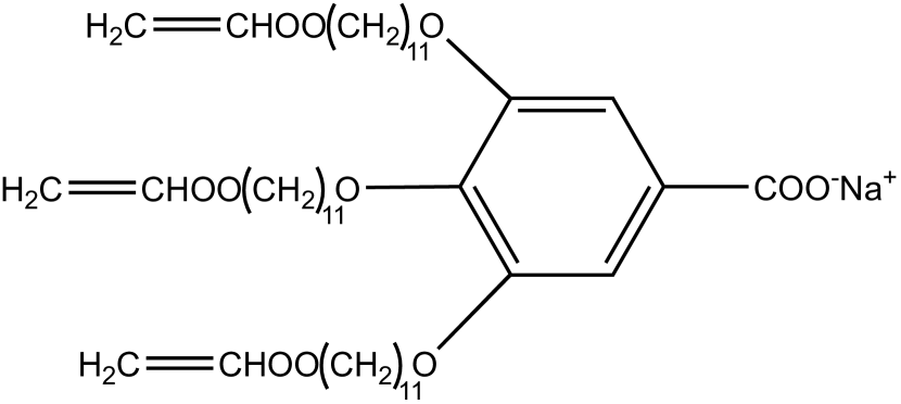
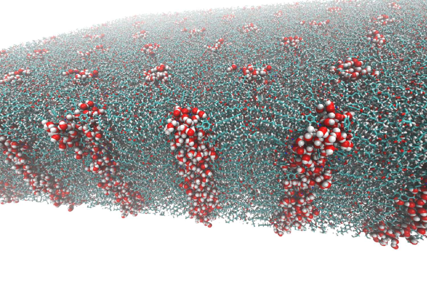
We studied transport of solutes in the HII phase using an atomistic molecular model of four pores in a monoclinic unit cell with 10% water by weight (see Figure 1). Approximately one third of the water molecules occupy the tail region with the rest near the pore center.
We chose to study a subset of the 4 fastest moving solutes from our previous work: methanol, acetic acid, urea and ethylene glycol. For each solute we created a separate system and to each system we added 6 solutes per pore for a total of 24 solutes. On the time scales which we simulate, this number of solutes per pore provides a sufficient amount of data from which to generate statistics. It also maintains a low degree of interaction between solutes since, at present, we are primarily interested in solute-membrane interactions. Further details on the setup and equilibration of these systems are described in our previous work.13
We extended the 1 s simulations of our previous work to 5 s in order to collect ample data. We ran MD simulations using the leapfrog integrator with hydrogen bonds constrained by the LINCS algorithm. We simulated a time step of 2 fs at a pressure of 1 bar and 300K controlled by the Parrinello-Rahman barostat and the v-rescale thermostat respectively. We recorded frames every 0.5 ns.
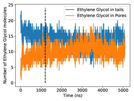
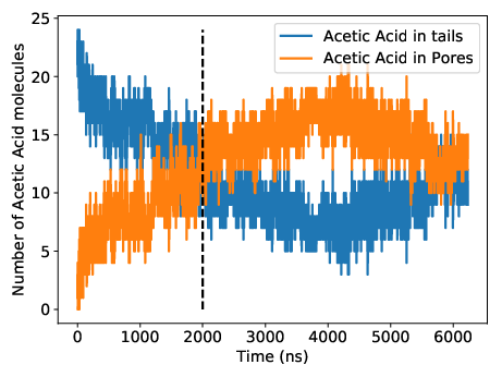
We considered each system to be equilibrated when the solute partitioning between the pore and tail region reached apparent equilibrium and use only data after that point in our analysis of solute kinetics. We plot the solute partition versus time in Figure 14 of the Supporting Information in order to justify our choice of equilibration times for each solute.
2.2 The Anomalous Diffusion Model
On the time scales simulated in this study, solutes in this system very clearly exhibit subdiffusive behavior, a type of anomalous diffusion. During an anomalous diffusion process, the mean squared displacement (MSD) does not grow linearly with time, but instead it follows a power law of the form:
| (1) |
where is the anomalous exponent and is the generalized diffusion coefficient. In this work, we only consider the MSD with respect to the solutes’ center of mass -coordinate, which is oriented along the pore axis. A value of indicates a subdiffusive process, while values of and are characteristic of Brownian and superdiffusive motion respectively.
While it is theoretically possible to extract the value of by fitting Equation 1 to an MSD generated directly from MD simulations, we do not simulate enough independent solute trajectories to obtain a reliable estimate. It is also possible that solute dynamics will become diffusive on long simulation timescales. Therefore, the transition from subdiffusion to regular diffusion may interfere with estimates of obtained by fitting to the MSD curves. We can obtain higher precision estimates of using the dwell time distributions as described in subsequent sections.
In this study, we primarily use the MSD as a tool for characterizing the average dynamic behavior of solute trajectories. Therefore, it is only important that we use a consistent definition for calculating the MSD between modeled trajectories and directly observed MD trajectories. We chose to calculate the time-averaged MSD from our MD simulations and stochastic models which measures all observed displacements over time lag :
| (2) |
where T is the length of the trajectory. In some situations, it may make more sense to use the ensemble MSD. We present further discussion of this choice in Section C of the Supporting Information.
2.2.1 Subordinated Fractional Brownian Motion
One can characterize the CTRW component of an sFBM process by the parameters which describe its dwell time and hop length distributions. We used the ruptures Python package in order to automatically identify mean shifts in solute trajectories, indicating hops.37 We used the corresponding hop lengths and dwell times between hops to construct empirical distributions.
Dwell time distributions: For subdiffusive transport, the distribution of dwell times is expected to fit a power law distribution proportional to . 38 Because we are limited to taking measurements at discrete intervals dictated by the output frequency of our simulation trajectories, we fit the empirical dwell times to a discrete power law distribution whose maximum likelihood parameter we calculated by maximizing the log likelihood function:
| (3) |
where , are collected dwell time data points, the total number of data points, and is the Hurwitz zeta function where is the smallest measured value of . 39
In practical applications, the heavy tail of power law distributions can result in arbitrarily long dwell times that are never observed in MD simulations. In order to directly compare our anomalous diffusion model to finite-length MD trajectories we need to bound the dwell time distribution. A standard way of doing this, with easily estimated parameters, is by adding an exponential cut-off to the power law so the dwell time distribution is now proportional to . 40, 39 We determine MLEs of and by maximizing the log likelihood function: 39
| (4) |
Correlated hop length distributions: The distribution of hop lengths by solutes undergoing an sFBM process is Gaussian, therefore we parameterize it by its standard deviation, . 21, 41, 42 The measured mean of the hop length distribution is always very close to zero so we assume that it is exactly zero in our time series simulations since we have no reason to expect drift in either direction based on pore symmetry.
sFBM implies that hops are correlated which we describe using the Hurst parameter, . The autocovariance function of hop lengths has the analytical form: 25
| (5) |
where is the variance of the underlying Gaussian distribution from which hops are drawn and is the time lag, or number of increments between hops. The hop autocorrelation function is simply Equation 5 normalized by the variance. When , hops are negatively correlated, when we recover Brownian motion and when , one observes positive correlation between hops. We obtained by performing a least squares fit of Equation 5 to the first ten 0.5 ns time lags of the empirically measured autocorrelation function (see section D of the Supporting Information for a more in depth justification of this method).
2.2.2 Subordinated Fractional Lévy Motion
Because we also want to account for the possibility that the distribution of hops is not Gaussian, we can model them with the more general class of Lévy stable distributions. For independent and identically distributed random variables, the generalized central limit theorem assures convergence of the associated probability distribution function (PDF) to a Lévy stable PDF. 24 The characteristic equation which describes the Fourier transform of a Lévy stable PDF is:
| (6) |
where
is the index of stability or Lévy index, is the skewness parameter, is the shift parameter and is a scale parameter. The most familiar case, and one of three that can be expressed in terms of elementary functions, is the Gaussian PDF ( = 2, = 0). We assume symmetric distributions centered about 0 implying that and are both 0.
For correlated hops, solute behavior may be described by subordinated fractional Lévy motion (sFLM). The Hurst parameter can again be used to describe hop correlations because they share the same autocorrelation structure. 43 The autocovariance function for FLM is:
| (7) |
where is the expected value of squared draws from the underlying Lévy distribution, effectively the distribution’s variance. 44 In general, most Lévy stable distributions have an undefined variance due to their heavy tails. However, normalizing Equation 7 by the variance of a finite number of draws from a Lévy stable distribution results in the same autocorrelation structure as FBM. See Section D of the Supporting Information for numerical simulations illustrating this point.
Analogous to power law dwell times, the heavy tails of Lévy stable hop length distributions result in rare but arbitrarily long hops. These long and unrealistic hops result in over-estimated simulated MSDs (see Figure 3(a) for example). We observe that the distribution of hops observed in our MD simulations are well approximated by Lévy stable distributions close to the mean, but they significantly under-sample the tails. We chose to truncate the Lévy stable distributions based on where the theoretical PDF starts to deviate from the empirically measured PDF (see Section E.1 of the Supporting Information). 45
Multiple Anomalous Diffusion Regimes
We observe different dynamical behavior when solutes move while inside the pore versus while in the tail region. This suggests two anomalous diffusion models of varying complexity. We first create a simple, single mode model with a single set of parameters fit to solute trajectories. Our second, two mode model assigns a set of parameters to each of 2 modes based on the solute’s radial location. We define the first mode as the pore region, defined as less than 0.75 nm from any pore center. Solutes outside the pore region are in the second mode, the tail region. We determined this cut-off by maximizing the difference in dynamical behavior as described in our previous work. 13 Unfortunately, there were not enough sufficiently long sequences of hops in each mode to reliably calculate a Hurst parameter for each mode so we used the single, average Hurst parameter from the single mode model for both modes of the two mode model.
For the two mode model, we defined a transition matrix describing the rate at which solutes moved between the tail and pore region. We assumed Markovian transitions between modes, meaning each transition had no memory of previously visited modes. We populated a 22 count matrix by incrementing the appropriate entry by 1 each time step and then generated a transition probability matrix by normalizing the entries in each row of the count matrix so that they summed to unity.
Simulating Anomalous Diffusion
We simulated models with all combinations of the types of dwell and hop length distributions described above, summarized in Table 1. All models include correlation between hops.
| Dwell Distribution | Hop Length Distribution | Abbreviation |
|---|---|---|
| Power Law | Gaussian | sFBM |
| Power Law w/ Exponential Cut-off | Gaussian | sFBMcut |
| Power Law | Lévy Stable | sFLM |
| Power Law w/ Exponential Cut-off | Lévy Stable | sFLMcut |
For each solute, we simulated 1,000 anomalous diffusion trajectories of length in order to directly compare our model’s predictions to MD simulations. varied between solutes due to differing solute equilibration times. We constructed trajectories by simulating sequences of dwell times and correlated hop lengths generated based on parameters randomly chosen from our bootstrapped parameter distributions. We propagated each trajectory until the total time equaled or exceeded s, then truncated the last data point so that the total time exactly equaled s since valid comparisons are only possible between fixed length sFBM simulations.
We used Equation 2 to calculate the time-averaged MSD of the MD and AD model trajectories then estimated their uncertainty using statistical bootstrapping. For each bootstrap trial, we randomly chose solute trajectories, where is the number of independent trajectories, with replacement, from the ensemble of trajectories and then calculated the MSD of the subset. We reported the time-averaged MSD up to a 1000 ns time lag with corresponding 1 confidence intervals.
When simulating 2 mode models, we determined the state sequence based on random draws weighted by the appropriate row of the probability transition matrix. We then drew hops and dwells based on the current state of the system. Since we calculated the transition probabilities from a finite data set, they have an associated uncertainty which we incorporated by re-sampling each row from a two dimensional Dirichlet distribution (which is also a beta distribution for the 2D case) with concentration parameters defined by the count matrix. 46
We used the Python package fbm 47 to generate exact simulations of FBM and our own Python implementation (see Table 3 of the Supporting Information) of the algorithm by Stoev and Taqqu to simulate FLM. 48 Note that, to our knowledge, there are no known exact simulation algorithms for generating FLM trajectories. However, the algorithm we used sufficiently approximates draws from the marginal Lévy stable distribution and reasonably approximates the correlation structure on MD simulation timescales. We added an empirical correction to enhance the accuracy of the correlation structure (see Section E.2 of the Supporting Information for validation of the approach).
2.3 The Markov State-Dependent Dynamical Model
A Markov state model (MSM) decomposes a time series into a set of discrete states with transitions between states defined by a transition probability matrix, . describes the conditional probability of moving to a specific state given the previously observed state. 49, 50
In this work, we define a total of 8 discrete states based on the 3 trapping mechanisms observed in our previous work. Therefore, there is no need to apply any algorithmic approaches to identify and decompose our system into discrete states. The states we have chosen include all combinations of trapping mechanisms in the pore and out of the pore (see Table 2). They assume that there are no significant kinetic effects resulting from solute conformational changes or pore size fluctuations. We use the same radial cut-off (0.75 nm) as in the AD approach to differentiate the pore and tail region. We define a hydrogen bond to exist if the distance between donor, D, and acceptor, A, atoms is less than 3.5 Å and the angle formed by is less than 30. 51 We define a sodium ion to be associated with an atom if they are within 2.5 Å of each other, as determined in our previous work. 13
| Markov State-Dependent Dynamical Model State Definitions | |
|---|---|
| 1. In tails, not trapped | 5. In pores, not trapped |
| 2. In tails and hydrogen bonding | 6. In pores and hydrogen bonding |
| 3. In tails and associated with sodium | 7. In pores and associated with sodium |
| 4. In tails, hydrogen bonding and associated | 8. In pores, hydrogen bonding and associated |
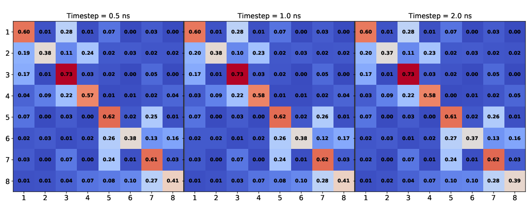
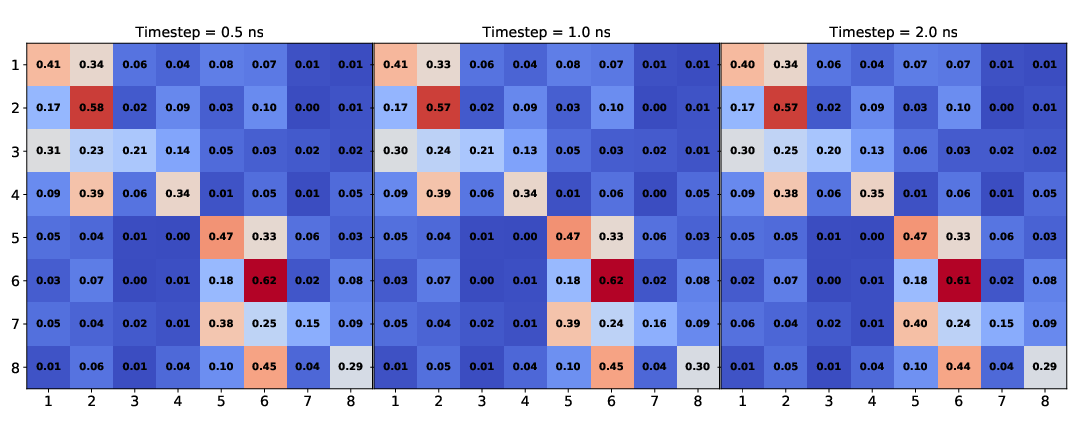
We constructed the state transition probability matrix, , based on observed solute trajectories. Using methods described in our previous work, we determined each solute’s radial location and which, if any, trapping mechanisms affected it at each time step, then assigned the observation to a specific state according to the definitions in Table 2. 13 Analogous to the mode transition matrix in Section 2.2, and based on the current and previous state observation, we incremented the appropriate entry of an count matrix by 1, where is the number of states. We verified the Markovianity of state transitions as described in Section F of the Supporting Information.
Adding to the standard MSM framework, we incorporated the dynamics of the solutes within each state as well as the dynamics of state transitions, which includes the overall configurational state of the solute and it’s environments. While MSMs are often used to estimate equilibrium populations of various states, adding state-dependent dynamics allows us to simulate solute trajectories. Hence why we refer to them as Markov state-dependent dynamical models (MSDDMs).
We recorded the -direction displacement at each time step in order to construct individual emission distributions for each state and transition between states. This results in 64 distinct emission distributions with some far more populated than others. We modeled all of the emission distributions as symmetric Lévy stable distributions in order to maintain flexibility in parameterizing the distributions.
We use the Hurst parameter to describe negative time series correlation. However, there is not sufficient data to accurately measure a Hurst parameter for each type of transition. We avoided this problem by combining all distributions associated with state transitions and treating all transitions as correlated emissions from a single Lévy stable distribution. This reduces the number of emission distributions from 64 to 9 (1 for each of the 8 states and 1 for transitions between states).
We simulated realizations of the MSDDM using the probability transition matrix and emission distributions. For each trajectory simulated, we chose an initial state randomly from a uniform distribution. We generated a full state sequence by randomly drawing subsequent states weighted by the rows of the probability transition matrix corresponding to the particle’s current state. Again, because we are working with a finite data set, we incorporated transition probability uncertainties into the rows of the transition matrix by resampling them from a Dirichlet distribution. For each same-state subsequence of the full state sequence, we simulated an FLM process using the Hurst parameter of that state and the parameters of the corresponding emission distribution. Independently, we simulated the transition between each same-state sequence with an FLM process based on the Hurst parameter of transition sequences and the parameters of the single transition emission distribution. We used the same FLM simulation procedure described in Section 2.2.
2.4 Estimating Solute Flux
We determine the rate at which solutes cross macroscopic-length pores based on the Hill relation: 52
| (8) |
where is the single particle solute flux and MFPT refers to the mean first passage time. To account for input concentration dependence of the flux, assuming that particles are independent, one can multiply Equation 8 by the total number of particles to get the total flux. In the context of our work, the MFPT describes the average length of time it takes a particle to move from the pore entrance to the pore exit.
We generated particle trajectories, parameterized with the above models, in order to construct a distribution of first passage times across a membrane pore of length . For each pore length, we simulated 10,000 realizations of an AD approach model all released at the pore entrance (). In the case of uncorrelated hops, one can continuously draw from the hop length distribution until (or for the sake of computational efficiency). The length of time between the last time the particle crossed and the end of the trajectory gives a single passage time. When particle hops are correlated, as they are in all cases of this work, we cannot continuously construct the particle trajectories. Rather, we must generate trajectories of length and measure the length of the sub-trajectory which traverses from to without becoming negative.
We calculated the expected value of analytical fits to the passage time distributions in order to determine the MFPT for a given solute and pore length. One should not use the mean of the empirical passage time distribution because it is highly likely that the true MFPT will be underestimated unless 100% of a very large number of trajectories reach . If a trajectory does not reach within steps, it is possible that a very long passage time has been excluded from the distribution.
To derive an analytical equation describing the passage time distributions, one can frame the problem as a pulse of particles instantaneously released at the pore inlet () which moves at a constant velocity, , and spreads out as it approaches . This spreading is parameterized by an effective diffusivity parameter, . This approach gives results equivalent to if we had released each particle individually and then analyzed the positions of the ensemble of trajectories as a function of time. The analytical expression describing the distribution of first passage times is: 53
| (9) |
where the only free parameters for fitting are and . A derivation of Equation 9 is given in Section G of the Supporting Information. We calculated the expected value of Equation 9 in order to get the MFPT.
We used the ratio of solute fluxes in order to determine membrane selectivity, , towards solutes. Selectivity of solute versus is defined in terms of the ratio of solute permeabilities, : 54
| (10) |
We can relate this to solute flux using Kedem and Katchalsky’s equations for solvent volumetric flux, , and solute flux, : 55, 56
| (11) |
| (12) |
where is the pure water permeability, and are the trans-membrane hydraulic and osmotic pressure differences, is the reflection coefficient, is the solute permeability, is the trans-membrane solute concentration difference and is the mean solute concentration. Since our simulations do not include convective solute flux, we eliminate the second term of Equation 12 which allows us to derive a simple expression for selectivity in terms of solute flux:
| (13) |
3 Results and Discussion
3.1 Anomalous Diffusion Modeling
3.1.1 Parameterizing Subordinated Fractional Brownian Motion
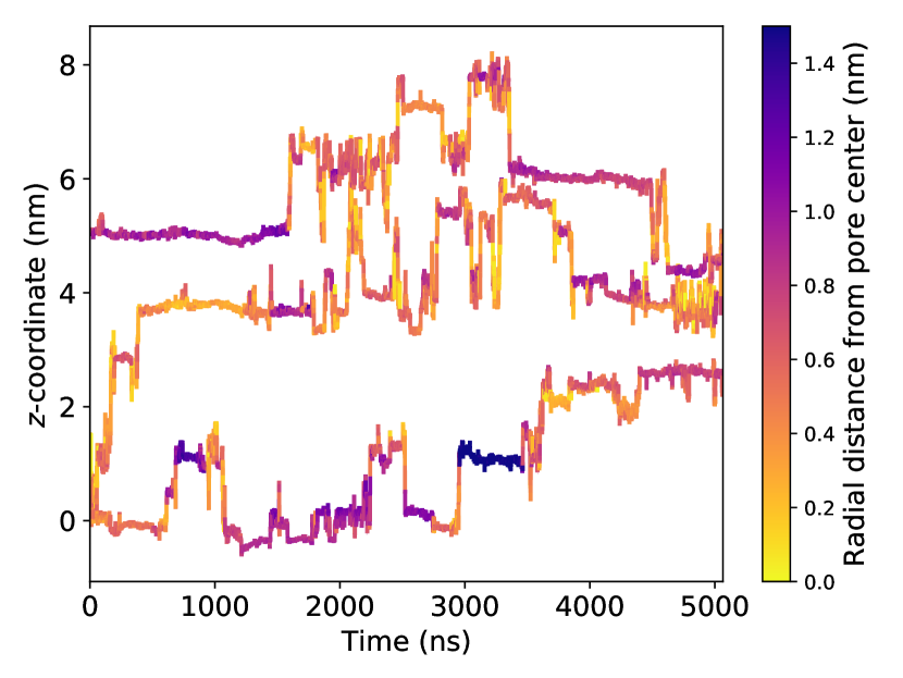
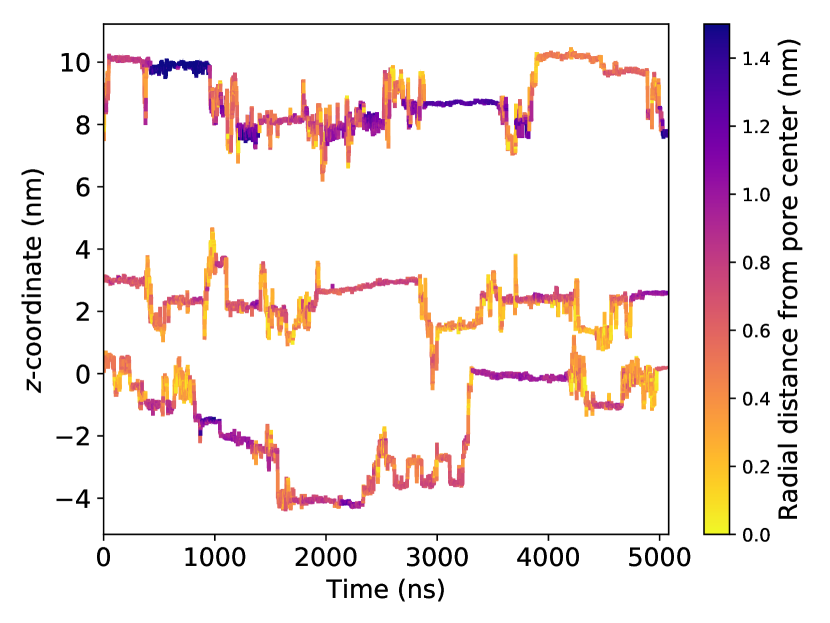
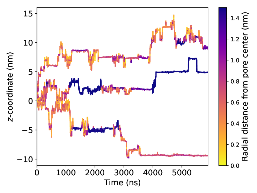
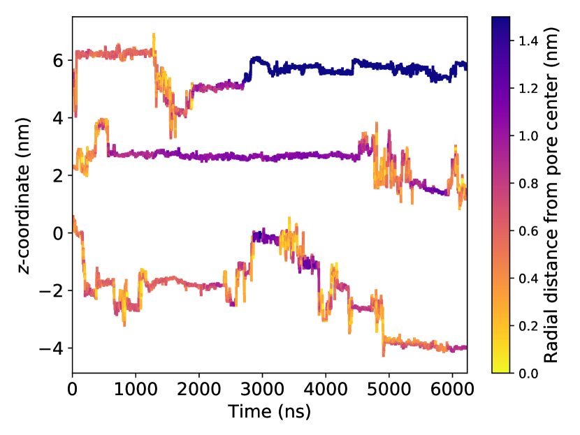
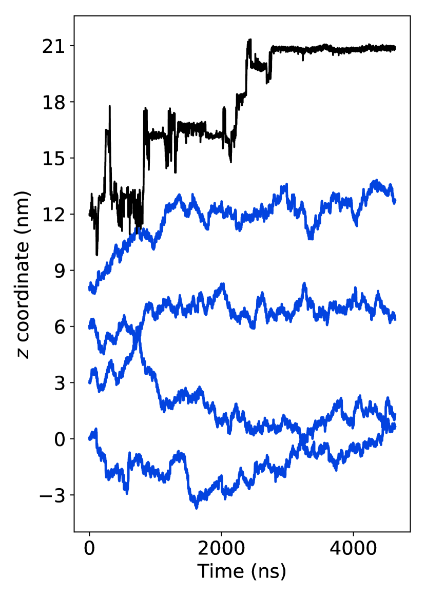
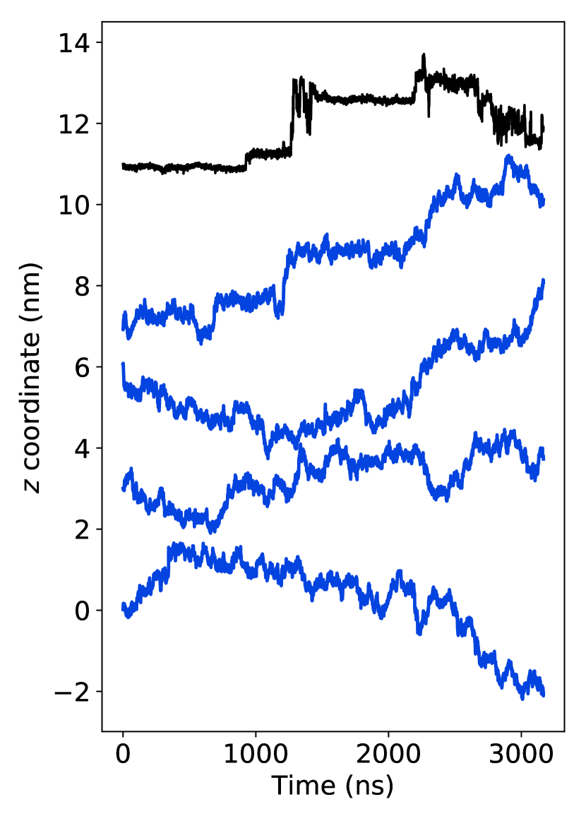
We find the data suggests that solute motion in this system can be well-modeled by subordinated fractional Brownian motion. In Figure 2, we plotted representative trajectories for each solute. They are characterized by intermittent hops between periods of entrapment. The near-Gaussian distribution of jump lengths and power law distribution of dwell times are both characteristic of CTRWs (See Figure 20 of the Supporting Information). Anti-correlation between hops suggests a fractional diffusion process is subordinate to the CTRW. Of the different models, a process subordinated by FBM or FLM is best supported by the data because the analytical correlation structures of hop lengths are close to those observed in our simulations (See Figure 20 of the Supporting Information). Fractional motion is common in crowded viscoelastic environments where motion is highly influenced by the movement of surrounding components, such as monomer tails in our case. 57
We modeled the distributions of hop lengths in two ways. First, we assumed the distribution to be Gaussian since it is possible to exactly simulate realizations of fractional Brownian motion. Second, we fit the distributions to Lévy stable distributions since it is more general than the Gaussian distribution. We plotted the MLE fits of both on top of each solute’s hop length distribution in Figure 20 of the Supporting Information. The Lévy distribution does a better job capturing the somewhat heavy tails and high density near 0 of the hop length distributions. However, since there are no known exact simulation techniques for generating realizations of fractional Lévy motion, this more general fit may not be worthwhile. In fact, we typically observe very little difference between model predictions parameterized with FLM versus FBM.
We also modeled the distribution of dwell times in two ways. First, we assumed pure power law behavior since it is consistent with most theoretical descriptions of CTRWs. The data fits well to this model at short dwell times but the density of long dwell times is over-estimated. In our second approach, we truncate the power law distribution with an exponential cut-off, lowering the probability of extremely long dwell times. On long time scales, the density of the truncated power law drops below that of the pure power law and tends towards 0.
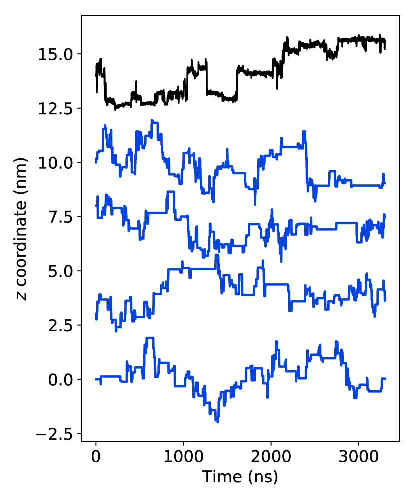
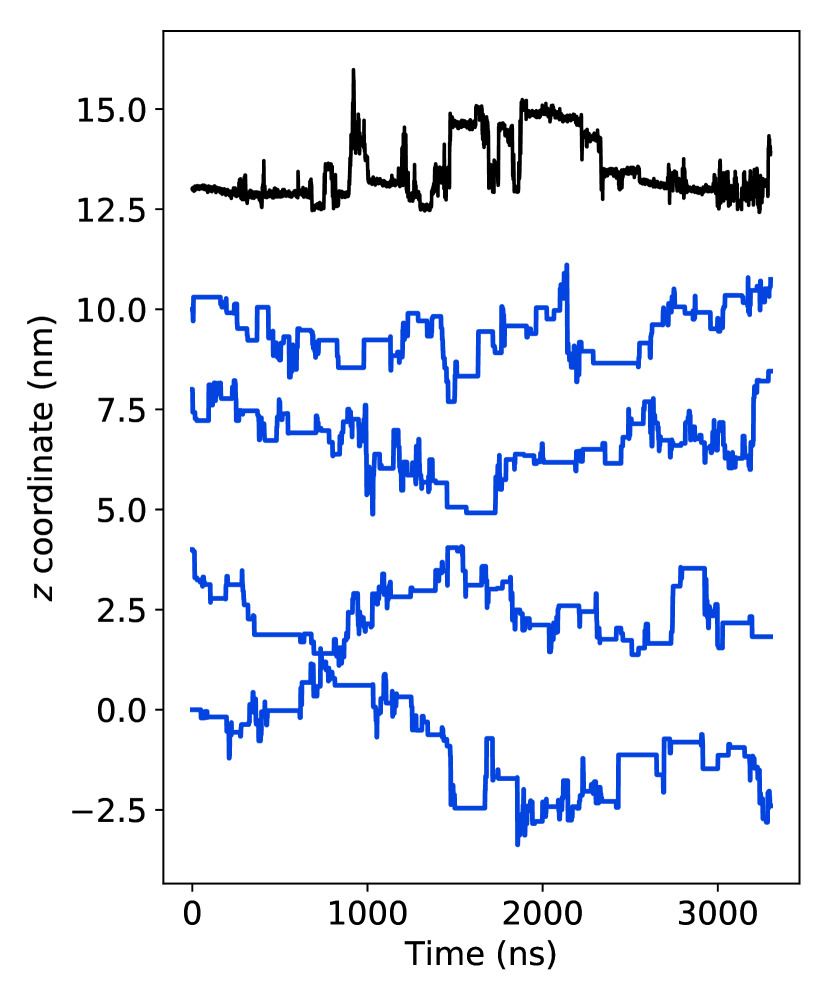
Several of the choices of AD models and parameters we have described yield qualitatively similar trajectories to those seen in our MD simulations. In Figure 3, we plot representative sample trajectories for each combination of the dwell time and hop distribution, labeled according to Table 1. The sFBMcut and sFLMcut in particular resemble the trajectories in Figure 2. When we do not truncate the dwell time distribution, the trajectories tend to incorporate very long dwell times as shown by the sFBM and sFLM models. Predictions made with these models consistently under-predict the MD MSDs (see Figure 21 of the Supporting Information). Therefore, we will not include the pure sFBM or sFLM models in the remainder of our analysis.
3.1.2 Model predictions
We obtain reasonable predictions of the MD simulated MSDs when we parameterize AD models with all available data after the perceived equilibration time. We observe that in some cases, solute trajectories extracted from our MD simulations may display non-stationary behavior. Our brief analysis in Section J of the Supporting Information suggests that we may be operating on the border of the minimum amount of data required to accurately parameterize AD approach models. The MSD curves generated from both the one and two mode models are overlaid with the MD simulated MSDs for comparison in Figure 4. The associated parameters for the one and two mode models are presented in Figures 5 and 6.
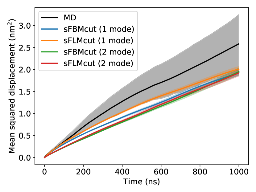
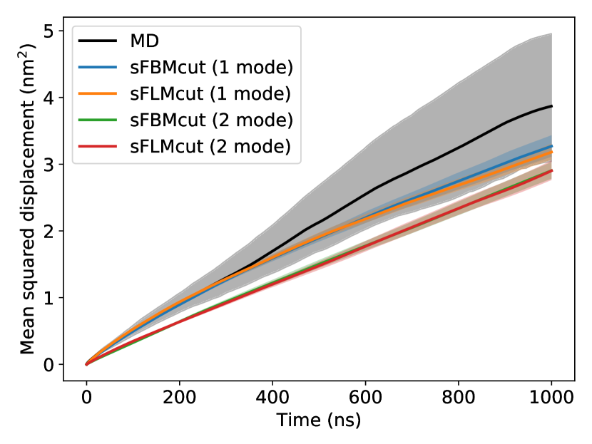
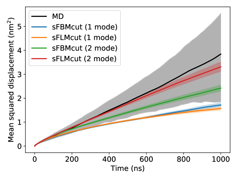
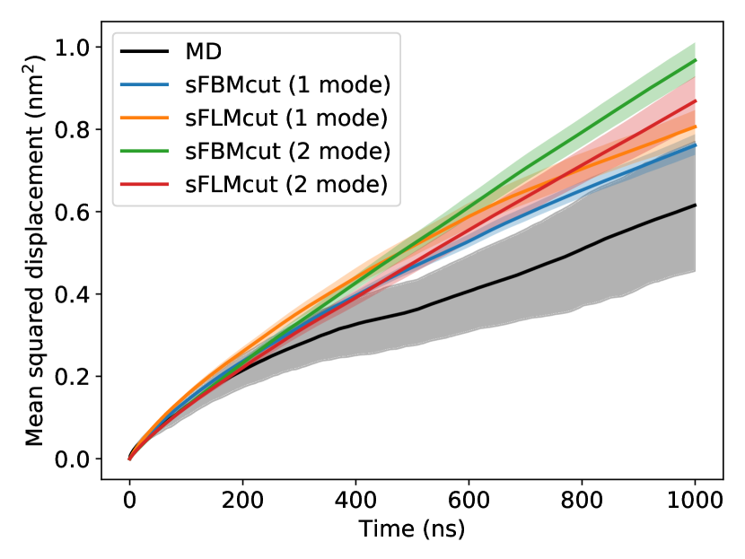
The one and two mode AD models do a fairly good job of predicting the magnitude of the MD MSD curves examined up to a 1000 ns time lag. In most cases, both the Brownian (sFBMcut) and Lévy (sFLMcut) versions of both the one and two mode AD models give very similar results, because the hop length distributions are nearly Gaussian even when fit to a more general Lévy distribution ().
The deviation between the one mode MSD predictions and MD are primarily due to differences in their curvature at long time lags. The shape and magnitude of the predicted curves appears accurate relative to MD at short time lags. However, the modeled trajectories undershoot the mean MD MSD as the time lag increases. Long time positional anti-correlation, on the order of hundreds of ns, may not exist in the MD system. Eventual loss of correlation would result in a shift from sub-linear, or subdiffusive, to linear, or diffusive, MSD behavior, as observed in the MD trajectories. Acetic acid exemplifies this point. At first glance, acetic acid’s predicted MSD appears to match the curvature of MD quite well, but closer examination reveals that the MD MSD curve may actually shift from a sub-linear to a linear regime around 500 ns.
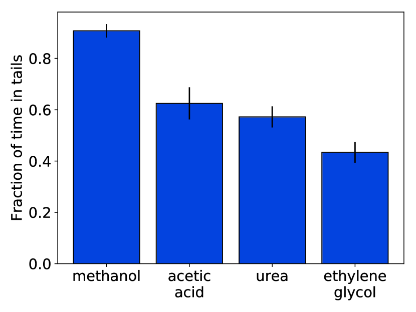
The two mode models display curvature more consistent with MD but for non-physical reasons. Every time a switch between the pores and tails occurs, the width of the distribution used to model hops changes, and the correlation structure is broken. Solutes that switch between modes the least show predicted MSDs with the greatest curvature. Due to the much larger accessible volume that a smaller molecule has, methanol spends of its time in the hydrophobic tails (see Figure 6(c)), so mode transitions are relatively rare and the predicted MSDs have significant curvature. This artificially resolves the problem of long timescale correlation, however, it has no physical basis.
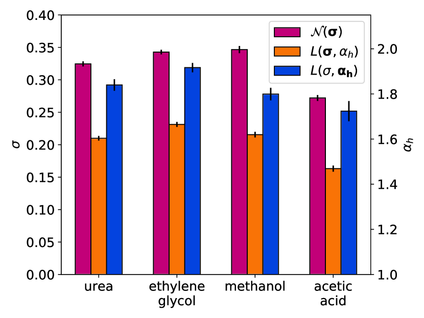
The model parameters for the one and two mode models tell stories about each solute’s behavior that help explain the difference between the MSDs of different solutes. Higher values of and lower values of indicate larger average hop length magnitudes by increasing the hop length distribution’s width and tail density respectively. Higher values of indicate a lower probability of long dwell times. Higher values of truncate the power law distribution earlier preventing extremely long dwell times. Values of closer to the Brownian limit of 0.5 indicate a lower degree of negative correlation between hops. All of these changes in physical behavior contribute to an overall increase in the predicted MSD.
Examining first the parameters of the one mode model, we can begin to break down the trends in solute MSDs. The parameters belonging to ethylene glycol and methanol are relatively similar, which is consistent with their similar MD MSDs and qualitatively similar MD time series. Relative to ethylene glycol, methanol tends to stay trapped for less time and takes larger hops but the most substantial difference is with respect to their Hurst parameters. Methanol has the lowest of all the solutes studied because it spends the majority of its time outside the pore region where collisions with tails are frequent. Urea has the third highest MSD which is primarily a consequence of more frequent and longer dwell times (lower and ). Urea’s hop lengths () and correlation () are comparable to ethylene glycol and methanol. Acetic acid has the smallest MSD among the solutes studied due to longer periods of entrapment and shorter hops. Its trapping behavior is parameterized by an value significantly lower than other solutes, but an intermediate value, suggesting it experiences many medium-length periods of entrapment. Its hops are smaller but are slightly compensated by a heavier tailed distribution (lower ) than the other solutes.
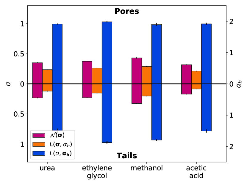
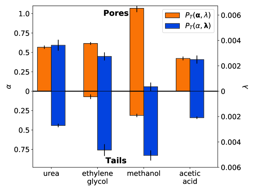
We can use the two mode model to gain an even deeper understanding of solute behavior in the pore versus in the tails. It is clear that solutes are significantly slowed while they are in the tail region where long dwell times are more probable (smaller ) and hops are smaller (smaller ). Each solute spends a different amount of time in the tails (see Figure 6(c)). Urea and acetic acid spend slightly more than half of their time in the tails (56% and 62% of their time respectively) while ethylene glycol spends about 44% of its time in the tails. Urea and acetic acid’s compact, flat structure allows it to more easily partition into the tails while ethylene glycol prefers the pore region due to its two hydrophilic hydroxyl groups. In contrast, methanol spends 91% of its time in the tails, likely due to its small size. The value of for urea and acetic acid in the tails is 1.50, meaning its hop distribution is heavy tailed relative to ethylene glycol and methanol, whose values are 1.90 and 1.85 respectively, which is more consistent with a Gaussian distribution (=2). Acetic acid and urea are structurally similar molecules, both planar with two heavy atoms attached to a carbonyl group. Their small size and rigid shape may allow them to occasionally slip through gaps in the tails. Meanwhile, methanol is small enough that it does not need to make larger jumps to escape traps.
Overall, the AD approach does a reasonable job of predicting solute MSDs and its parameters can help us further understand solute dynamics. Hops appear to be well modeled as anti-correlated draws from either Gaussian or Lévy stable distributions. The data strongly suggests that one must truncate the power law dwell time distributions in order to obtain accurate MSD estimates. Trajectories generated by pure power laws are qualitatively non-physical. We can further understand solute dynamics by adding radially dependent parameter distributions as in the 2 mode model. A significant amount of solute trajectory data is necessary in order to achieve good parameter estimates.
3.2 The Markov State-Dependent Dynamical Model
The AD model is useful if one does not know exact transport mechanisms in a system since it only requires time series data. However, since we have already studied transport mechanisms in detail in our previous work, we can attempt to model transport as transitions between known discrete states, defined in Table 2, with state-dependent positional fluctuations, which we refer to as the Markov state-dependent dynamical model (MSDDM).
3.2.1 Solute state preferences
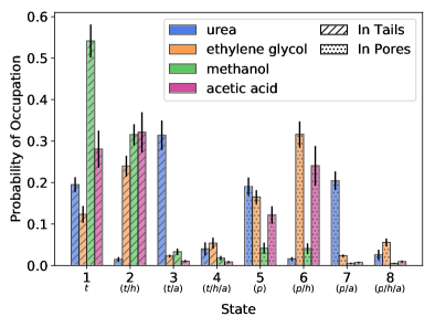
Solute size and chemical functionality influence which states are visited most frequently. In Figure 7, we plotted the probabilities of occupying a given state at any time. Solutes tend to favor the same types of interactions independent of which region they are in. We can relate these interactions to solute chemical functionality and use that intuition to hypothesize new designs for LLC monomers which control the transport rate of specific solutes.
-
•
Urea spends the largest fraction of its time trapped via association with sodium ions. It does so 31% of the total time while in the tails (state 3) and 21% of the total time while in the pores (state 7). Note that sodium does not drift significantly into the tails but sits close to the pore/tail region boundary. The electron-dense and unshielded oxygen atom of urea’s carbonyl group is prone to associate with positively charged sodium ions. The nitrogen atoms of urea are only weak hydrogen bond donors. Therefore, the transport rate of urea is likely to be most significantly modified by removing or changing the identity of the counter-ion.
-
•
Ethylene glycol spends the largest fraction of its time trapped in a hydrogen bonded state. It does so 24% of the total time while in the tails (state 2) and 32% of the total time while in the pores (state 6). The two hydroxyl groups of ethylene glycol readily donate their hydrogen atoms to the carboxylate head groups and the ether linkages between the head groups and monomer tails. The transport rate of ethylene glycol might be modified by removing hydrogen bond accepting groups from the LLC monomers, especially those which stabilize the solute in the tails (i.e. the ether linkages).
-
•
Methanol spends most of its time unbound in the tail region (state 1) and spends a significant portion of time hydrogen bonded while in the tail region. Tail region hydrogen bonds are donated from methanol to the ether linkages between the monomer head groups and tails, as well as to the ester groups at the ends of the tails. One might modify the rate of methanol transport by controlling its partition into the monomer tails. This might be achieved by adding cross-linkable groups near the monomer head groups.
-
•
Acetic acid spends the majority of its time hydrogen bonding both in and out of the pore (states 2 and 6). Although it has an unshielded carbonyl group in its structure, association with sodium ions in this environment is apparently a much weaker interaction than hydrogen bonding. As with ethylene glycol, one might modify the transport rate of acetic acid by removing hydrogen bond accepting constituents of the LLC monomer. With this modification, we hypothesize that acetic acid might show similar transport rates to urea given their structural similarity.
3.2.2 Parameters of the MSDDM
To create an MSDDM for each solute, we determined the state sequence associated with each solute trajectory based on the geometric indicators of the states indicated in Table 2. We then generated emission distributions of fluctuations within each state as well as transitions between states. In theory, one could parameterize separate transition distributions for those which occur in the tails versus in the pores, however this would lead to a broken correlation structure similar to that seen in the two mode AD models.
We observe correlated emissions drawn from Lévy stable distributions. The deviation of the emission distributions from Gaussian behavior is far more pronounced than that seen in the hop length distributions of the previous section (see Figure 25(a) of the Supporting Information). We therefore did not consider the Gaussian case. The correlation structure between hops is consistent with that of FLM (see Figure 25(b)). The parameters of the Lévy stable distributions along with their Hurst parameters are visualized in Figure 8 (and tabulated in the Supporting Information, Table 6).
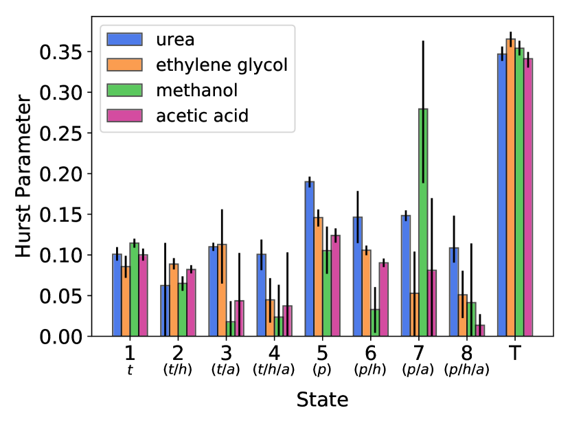
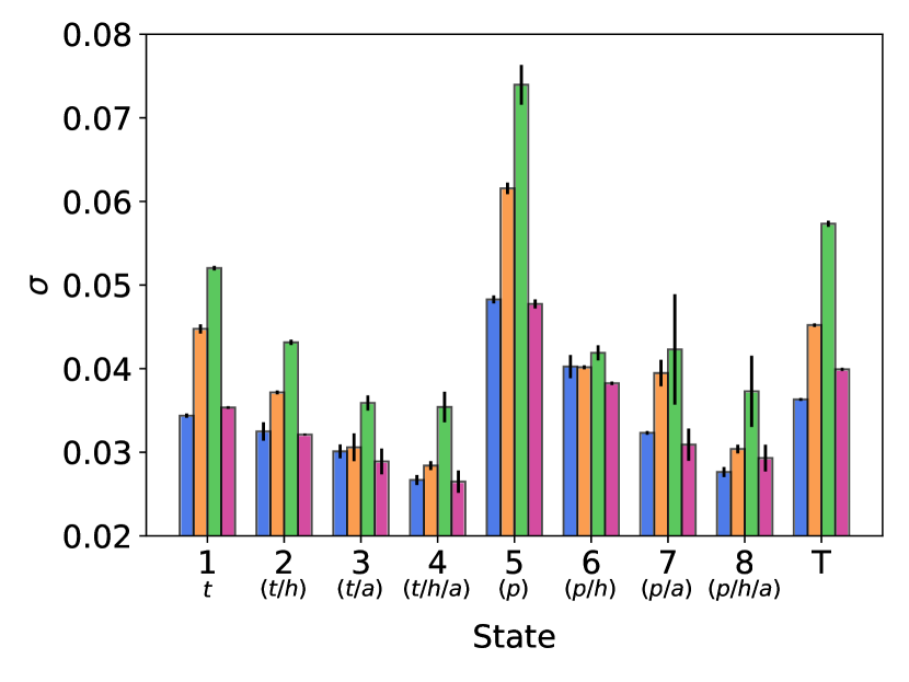
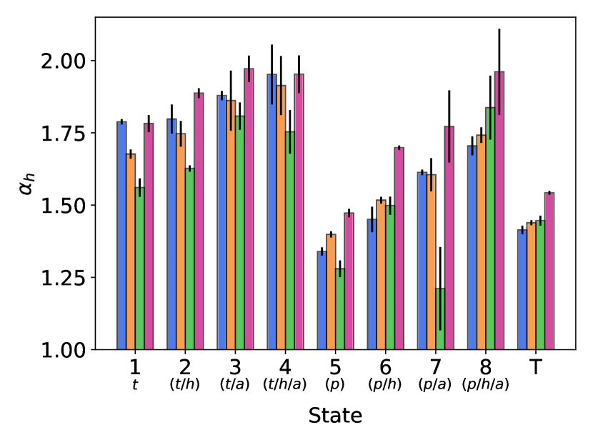
Most of a solute’s MSD is a consequence of transitions between the 8 states in Table 2. Perfectly anti-correlated motion (=0) results in no contribution to the solute’s MSD. Motion while trapped in a state is highly anti-correlated as indicated by their consistently low Hurst parameters. There is a weak negative trend in the Hurst parameter values as the number of simultaneously influencing trapping mechanisms increases (Figure 8(a)). The Hurst parameters for transitional (T) emissions are up to 18 times higher than emissions from trapped states. The value of for transition emissions is also relatively low giving higher probabilities to larger hops.
As solutes are influenced by more trapping interactions simultaneously (e.g. hydrogen bonding and association with sodium versus just hydrogen bonding), the width of the hop length distribution, , decreases while its Lévy index, , increases. Treating states in the tail and pore regions independently, is largest and is smallest when solutes are not hydrogen bonding or associating with sodium (states 1 and 5). Solutes are free to move and take occasionally large hops. The smallest and highest values are measured when solutes are hydrogen bonding and associating with sodium at the same time (states 4 and 8). Motion is restricted by multiple stabilizing forces which maintains a relatively narrow distribution of hop lengths.
3.2.3 Application of the MSDDM
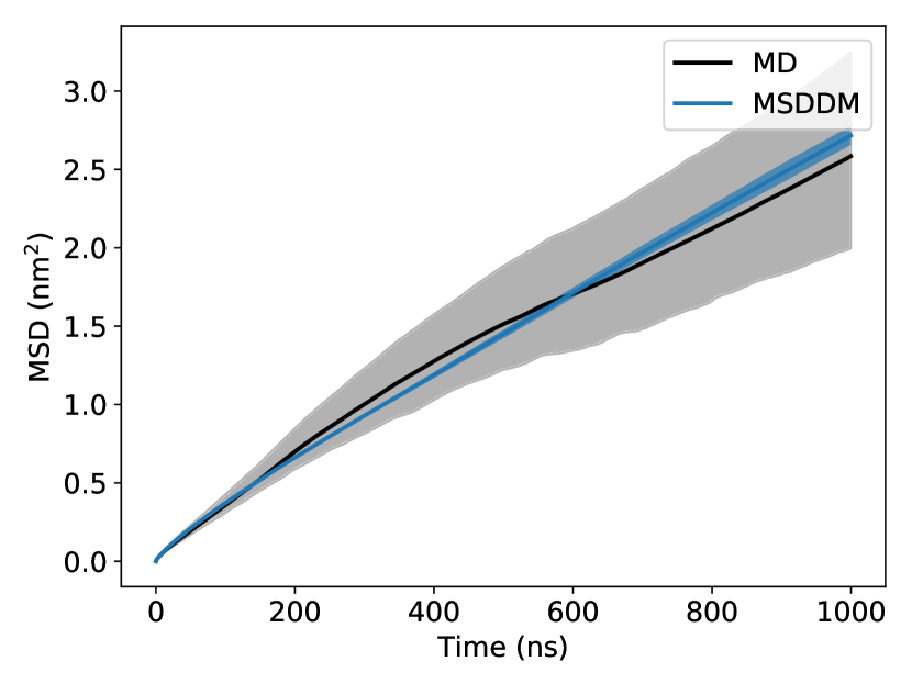
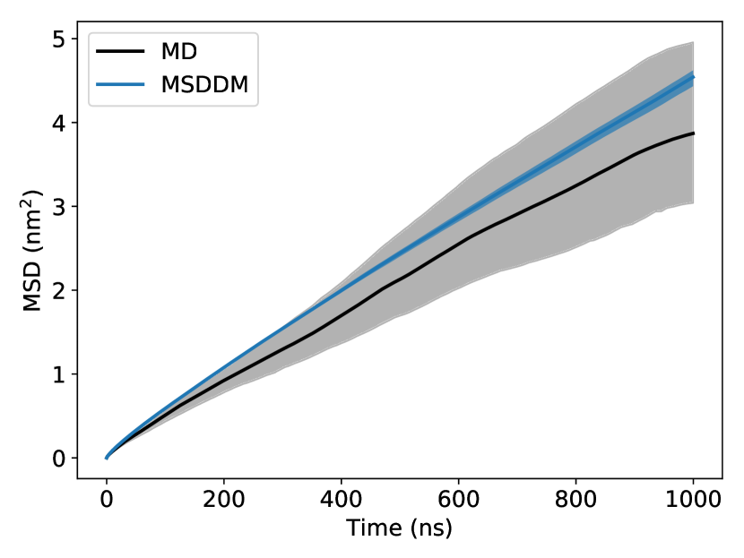
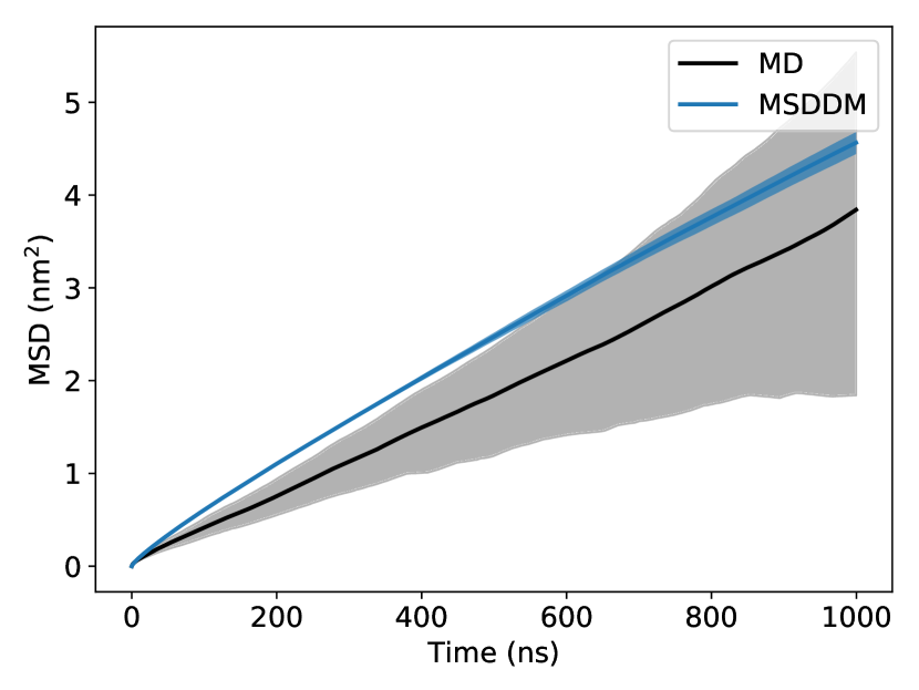
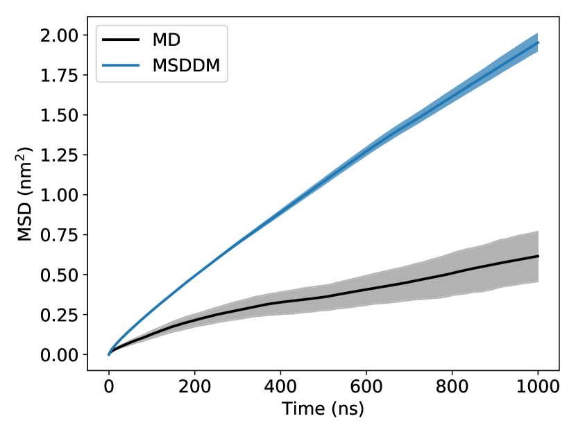
Quantitatively, the dynamics of urea, ethylene glycol and, to a lesser extent, methanol appear to be well-captured by the MSDDM. We simulated 1000 MSDDM trajectory realizations for each solute, as described in Section 2.3, then calculated their MSDs (see Figure 9). In most cases, the MSDDM predicts the magnitude of the MD MSDs within their 1 confidence intervals.
The predicted MSD of acetic acid is severely over-estimated primarily due to under-estimation of hop anti-correlation ( too high) and an over-estimate of its hop lengths ( and too high). Acetic acid’s predicted MSD actually lies just within the lower bound of urea’s MD MSD 1 confidence interval, but lower than the prediction of the MSDDM for urea. As stated earlier, most of a solute’s motion modeled by the MSDDM is due to displacements during state transitions. Acetic acid has a transitional Hurst parameter close to urea’s and transitional and values that are higher than urea’s. The primary reason that the MSDDM predictions for acetic acid’s MSD are lower than urea’s appears to be because of higher hop anti-correlation (lower ) in all states, including transitions. There is also the strong possibility that the over-estimate is a consequence of lumping together all of acetic acid’s transitional hops into a single correlated distribution.
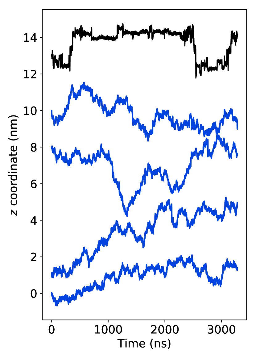
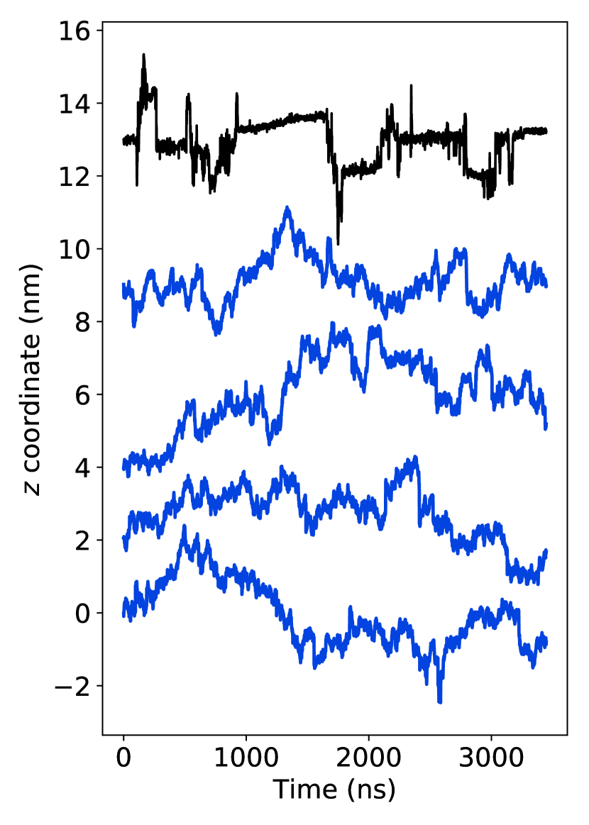
Despite relatively good predictions of the MD MSD, qualitative mismatch between simulated MSDDM and MD trajectories suggest that the MSDDM may be getting the right answers for the wrong reasons. We plotted typical realizations of the MSDDM for each solute and compared them to MD in Figure 10. There is little evidence of trapping behavior or large hops. There are two reasons for this behavior. First, the width of hop length distributions are much smaller than those of the AD model. Closer examination of the characteristic MD trajectories shown in Figure 2 reveal that hops tend to be an accumulation of a series of hops in the same direction. All of the hops in the MSDDM are negatively correlated which prevents this from happening. The second reason is a consequence of using a single hop length distribution for transitions. This was necessary because we could not collect enough data to fit all of the possible transition distributions and because we could not correlate emissions coming from different hop distributions. Many transitions occur between two trapped states where the transitional hops are actually very small. Our model ignores this physical restriction which can cause the solute to drift rather than stay trapped.
3.3 Solute Flux and Selectivity
We used the one mode sFBMcut (see Table 1) AD model in order to demonstrate how one can use its realizations in order to calculate the flux (see section 2.4) of solutes given model parameters extracted from MD simulations. The one mode sFBMcut model generates predictions similar to the one mode sFLMcut model at a lower computational cost. We do not consider the two mode AD model because it has a broken correlation structure and we do not consider the MSDDM because its realizations do not display the expected hopping and trapping behavior.
It is computationally infeasible to simulate trajectories long enough that they traverse the length of a macroscopic pore. To date, the thinnest HII LLC membrane synthesized with the monomer in this work was 7m thick. 7 Using 24 cores to simulate trajectory realizations in parallel, it takes on the order of 1 day to simulate 10000 sFBMcut realizations of solutes traversing a 50 nm pore. The RAM requirements and performance scales greater than linearly and thus would take an infeasible amount of memory and time to simulate transport through a pore over 100 times longer. One could improve performance significantly by simulating less trajectories. In Figure 27 of the Supporting Information, we determined that one can simulate as few as 100 sFBMcut realizations in order to parameterize Equation 14. For better precision, we recommend simulating at least 1000 realizations. However, even with an order of magnitude decrease in number of trajectories, it is still infeasible to simulate experimental-length pores.
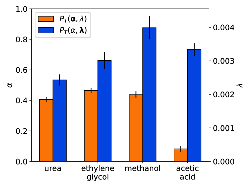
We used simulated trajectories which traverse computationally-reasonable length pores in order to construct an empirical model which one can use to estimate particle flux for arbitrary length pores. We fit Equation 9 to the empirical distribution of first passage times in Figure 11(a) and used the expected value of the analytical equation to calculate flux from Equation 8. As shown in Figure 11(b), the flux appears to scale according to a power law of the form:
| (14) |

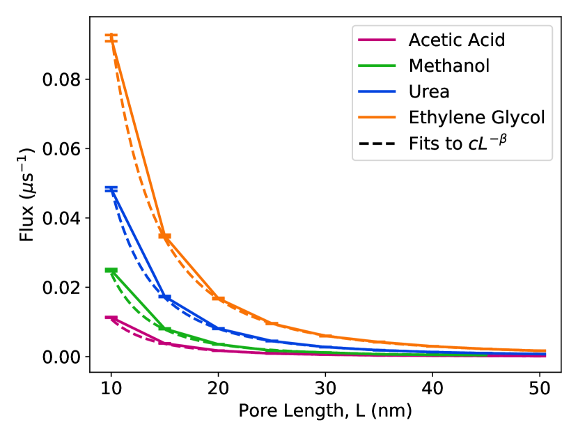
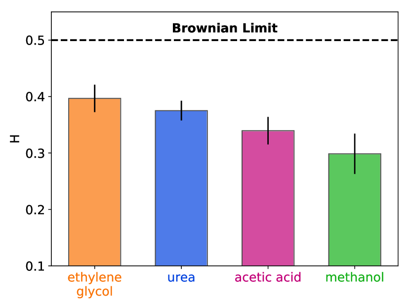
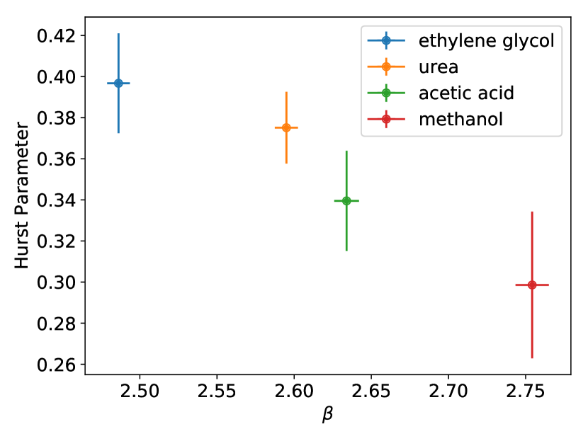
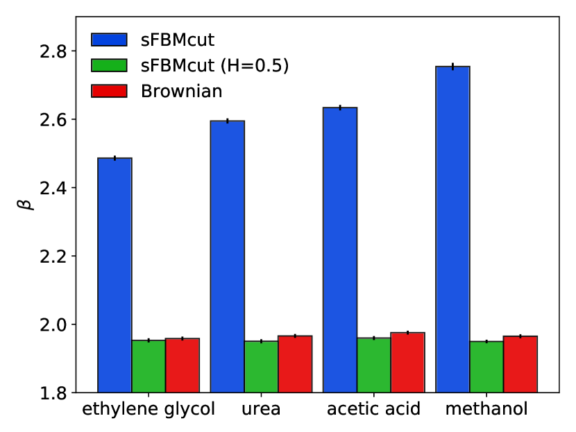
The scaling of solute flux with pore length is primarily influenced by anti-correlation between solute hops. In Figure 12a, we show that is inversely related to the Hurst parameter. This makes intuitive sense since higher degrees of anti-correlation should slow the rate at which solutes cross a membrane pore of a given length. When we remove anti-correlation between hops (set =0.5), the length dependence becomes the same for all solutes, dropping to a value just below 2. This also implies that hop lengths and dwell times do not affect length dependence since each solute exhibits different hopping and trapping behavior yet are all parameterized by the same value of when =0.5. We further verified this claim by removing hop anti-correlation and setting all dwell times equal to one timestep, effectively simulating Brownian motion. The length dependence remains unchanged.
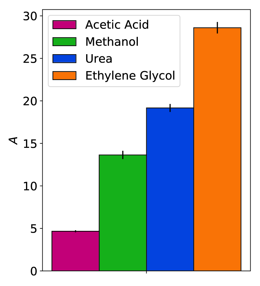
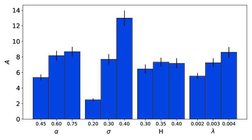
Dwell times and hop lengths directly modify the rate at which solutes move through the membrane pores and are reflected in the scaling pre-factor of the solute flux curves, . Comparison of Figure 12(c) with Figure 11(b) reveals that the ranking of the parameters is consistent with the ranking of solute flux. In Figure 12(d) we demonstrate that decreasing dwell times (increasing ), cutting off the dwell time distribution at shorter times (increasing ), and increasing hop lengths (increasing ) independently lead to an increase in . Figure 12(d) also suggests that is not dependent on hop anti-correlation ().
The power law decay of the flux with pore length implies the following relationship for selectivity via substitution of Equation 14 into Equation 13:
| (15) |
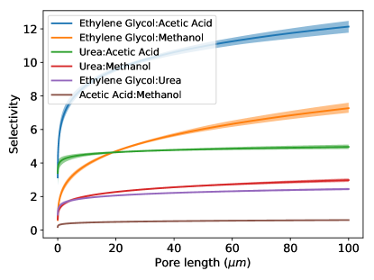
In Figure 13, we plot Equation 15 for pore lengths ranging from those studied in Figure 11(b) to macroscopic-length pores. For the same degree of hop anti-correlation, as is the case for uncorrelated motion, selectivity depends on solute hop lengths and dwell times (). For , LLC membranes will be more selective towards passage of solutes with less anti-correlated hopping behavior (lower ). The selectivity towards solutes with less length dependent flux increases with membrane thickness. In most cases, the length dependence of selectivity plateaus near or within the range of experimentally-accessible membrane thicknesses. Therefore, from a practical standpoint, one should not expect significant changes in selectivity by varying LLC membrane thickness.
Of the solutes studied, the data suggests that this particular LLC membrane might be most useful for selectively separating ethylene glycol from methanol and acetic acid. Relative to acetic acid, ethylene glycol takes larger hops and is trapped longer, leading to a larger . There is also an appreciable difference in the scaling of each solute’s flux with pore length () which gives the selectivity significant length dependence. Relative to methanol, ethylene glycol takes similarly-sized hops and dwells which is why selectivity is relatively low for very short pore lengths. However, the large difference in hop correlation between the two solutes leads to the strongest pore length dependence of selectivity.
The insights into flux and selectivity provided by our time series modeling approach could not be drawn easily by simply observing solute motion, the structure of the membrane nanopores, or even the solute trajectories extracted from the MD simulations. Differences in solute MSDs alone do not fully explain the trends and magnitudes of the selectivities shown in Figure 13. Complex interplay between membrane constituents and solutes with varying chemical functionality lead to diverse solute behavior. Even if our model is not perfect, it provides clear logic behind the mechanisms leading to selective behavior which could significantly help illuminate any design choices. We hope this type of analysis can be leveraged to explore new, interesting and complex separations problems.
4 Conclusions
We have tested two different mathematical frameworks for describing complex solute dynamics by applying them to an HII phase LLC membrane. The values obtained for the parameters when fitting the models to the time series data offer important mechanistic insight on the molecular details of transport. Subordinated fractional Brownian and Lévy motion have a strong theoretical foundation in the anomalous diffusion literature. Our single mode AD model quantifies and allows comparison of the hopping and trapping behavior among solutes. A two mode model that describes dynamics based on whether a solute is in or out of the pore region allows us to break down individual solute motion into two distinct regimes and we showed that solute motion is clearly restricted while in the tail region. Our Markov state-dependent dynamical model uses explicitly defined trapping mechanisms and gives a nice description of transitions between these observed states, the equilibrium distribution of solutes among states as well as the type of stochastic behavior shown in each state.
Although large portions of the MSDs predicted by our models fall close to or within the 1 confidence intervals of MD, it is not always for physically accurate reasons. Qualitatively, MSDDM trajectories do not display the same hopping and trapping behavior shown by MD trajectories. Frequent transitions drawn from a single, relatively broad transition emission distribution prevent long periods of immobility. The most obvious solution to this would be to generate individual emission distributions for each type of transition, but this would require orders of magnitude more data or more prior assumptions about the distributions. This approach is further complicated by the need to make correlated draws from a fractional Lévy process with a frequently changing distribution width. A possible simplification could be to assume that correlation is lost every time a state transition occurs.
Although the AD approach generates qualitatively accurate trajectories and predicts MSDs near or within the 1 confidence interval of our MD simulations, the curvature of the predicted MSDs does not appear to be consistent with the MD simulations. The MSD curves calculated from MD simulations appear to straighten out on long timescales while those predicted from the AD models continuously curve. This is because pure fractional Brownian motion features hop correlation that persists indefinitely. However, it is likely that on longer timescales, hops become decorrelated, causing solute dynamics to transition from subdiffusive to diffusive behavior. We may be able to incorporate this transition by truncating the positional autocorrelation function, allowing correlation to diminish on the 100 ns time scale as suggested by the physical trajectories.
We demonstrated how one could use the one mode AD model, or any stochastic time series model, in order to to determine macroscopic flux and selectivity. We showed that, when using the AD model, solute flux decreases with pore length at a rate faster than pure Brownian motion due to anti-correlation between hops. Due to differences in hop anti-correlation, we observe length dependent selectivity. Based on these calculations we can hypothesize that this particular LLC membrane may be a good candidate for the selective separation of ethylene glycol from acetic acid or methanol.
In a broader context, it is clear that time series modeling may be a useful way to form a clear connection between complex solute dynamics on the nanosecond timescale and macroscopic observables. On the nanoscopic scale, one can both learn and characterize dynamical modes in order to identify areas of potentially impactful molecular-level design changes. For example, it may be possible to modify solute transport rates and selectivities in LLC membranes by redesigning the LLC monomers to mitigate or enhance their chemically dependent interactions with different solutes. With these models, dynamics can be propagated onto much longer time with computational ease. This allows one not only to predict a macroscopic observable for a specific system, but to explicitly calculate the effect of perturbations to model parameters that may result from a monomer design change. Overall, we hope that this work can advance the reader’s understanding of how one can apply time series analysis in order to understand complex diffusive behavior in any system of interest.
Acknowledgments
We thank Richard Noble for helping us make the connection between the empirical mean first passage time distribution and the analytical equation to which we fit the distributions (Equation 9).
This work was supported in part by the ACS Petroleum Research Fund grant #59814-ND7 and the Graduate Assistance in Areas of National Need (GAANN) fellowship which is funded by the U.S. Department of Education. Molecular simulations were performed using the Extreme Science and Engineering Discovery Environment (XSEDE), which is supported by National Science Foundation grant number ACI-1548562. Specifically, it used the Bridges system, which is supported by NSF award number ACI-1445606, at the Pittsburgh Supercomputing Center (PSC). This work also utilized the RMACC Summit supercomputer, which is supported by the National Science Foundation (awards ACI-1532235 and ACI-1532236), the University of Colorado Boulder, and Colorado State University. The Summit supercomputer is a joint effort of the University of Colorado Boulder and Colorado State University.
Supporting Information
Appendix A Setup and analysis scripts
| Script Name | Section | Description |
|---|---|---|
| /setup/parameterize.py | 2.1 | Parameterize liquid crystal monomers and solutes with GAFF |
| /setup/build.py | 2.1 | Build simulation unit cell |
| /setup/place_solutes_pores.py | 2.1 | Place equispaced solutes in the pore centers of a unit cell |
| /setup/equil.py | 2.1 | Equilibrate unit cell and run production simulation |
| /analysis/solute_partitioning.py | 2.1 | Determine time evolution of partition of solutes between pores and tails |
| /timeseries/msd.py | 2.2 | Calculate the mean squared displacement of solutes |
| /analysis/sfbm_parameters.py | 2.2 | Get subordinated fractional Brownian motion parameters by fitting to a solute’s dwell and hop length distributions and positional autocorrelation function. |
| /timeseries/ctrwsim.py | 2.2 | Generate realizations of a continuous time random walk with the user’s choice of dwell and hop distributions |
| /timeseries/forecast_ctrw.py | 2.2 | Combines classes from sfbm_parameters.py and ctrwsim.py to parameterize and predict MSD in one shot. |
| /analysis/ Markov_state_dependent_dynamics.py | 2.3 | Identify frame-by-frame state of each solute, construct a transition matrix and simulate realizations of the MSDDM model. |
| /timeseries/mfpt_pore.py | 2.4 | Simulate mean first passage time distributions using the AD approach. |
All python and bash scripts used to set up systems and conduct post-simulation trajectory
analysis are available online at
https://github.com/shirtsgroup/LLC_Membranes.
Documentation for the LLC_Membranes repository is available at
https://llc-membranes.readthedocs.io/en/latest/. Table 3
provides more detail about specific scripts used for each type of analysis performed in
the main text.
Appendix B Solute Equilibration
We collected all data used for model generation after the solutes were equilibrated. We assumed a solute to be equilibrated when the partition of solutes in and out of the pore region stopped changing. The pore region is defined as within 0.75 nm of the pore center. We plot the partition versus time in Figure 14 and indicated the chosen equilibration time points.


Appendix C Mean Squared Displacement
In this study, we primarily use the MSD as a tool for characterizing the average dynamic behavior of solute trajectories. Rather than using them to calculate diffusion constants or to relate our simulations to experimental measurements, we compare MSDs calculated from MD simulations to those generated from our models in order to validate those models. Therefore, it is only important that we use a consistent definition for calculating the MSD between modeled trajectories and directly observed MD trajectories.
One can measure MSD in two ways. The ensemble averaged MSD measures displacements with respect to a particle’s initial position:
| (16) |
Fits to the ensemble averaged MSD will always reproduce the form of Equation 1 of the main text. The time-averaged MSD measures all observed displacements over time lag :
| (17) |
where T is the length of the trajectory.
The time averaged and ensemble averaged MSDs will give identical results unless a system displays non-ergodic behavior. For a pure CTRW, the power law distribution of trapping times leads to weak ergodicity breaking. In this case, the time-averaged MSD is linear while the ensemble averaged MSD has the form of Equation 1 of the main text. 38 With power law trapping behavior, the time between hops diverges so there is no characteristic measurement time scale of solute motion. In fact, as measurement time increases, the average MSD of a CTRW tends to decrease, a phenomenon called aging, because trajectories with trapping times on the order of the measurement time get incorporated into the calculation. 58
We chose to use just the time-averaged MSD to compare MD trajectories with modeled trajectories, because, compared to the ensemble average, it is a more statistically robust measure of the average distance a solute travels over time. The ensemble MSD of only 24 solute trajectories would have much higher uncertainties.
Appendix D Estimating the Hurst Parameter
We chose to estimate the Hurst parameter, by a least squares fit to the analytical autocorrelation function for fractional Brownian motion (the variance-normalized version of Equation 5 in the main text):
| (18) |
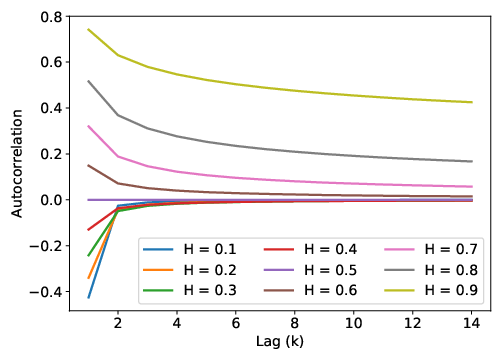
There are many methods for estimating the Hurst parameter for a time series. 59 It can be a difficult task because Equation 18 decays slowly to zero, especially when , meaning one needs to study large time lags with high frequency.
Fortunately, from a mathematical perspective, all of our solutes show anti-correlated motion, so most of the information in Equation 18 is contained within the first few time lags. In Figure 15(a), we plotted Equation 18 for different values of . When , Equation 18 decays slowly to zero meaning one needs to study large time lags with high frequency in order to accurately estimate from the data. However, when , the autocorrelation function quickly decays towards zero.
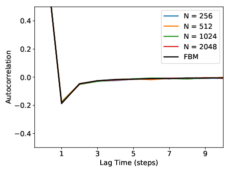
The autocovariance function of fractional Lévy motion is different from fractional Brownian motion (see Equations 5 and 7 of the main text), but their autocorrelation structures are the same. The autocovariance function of FLM is dependent on the expected value of squared draws from the underlying Lévy distribution, . This is effectively the distribution’s variance, which is undefined for most Lévy stable distributions due to their heavy tails. As a consequence, one should expect to grow as more samples are drawn from the distribution with the autocovariance function responding accordingly. However, we are only interested in the autocorrelation function. In order to predict the Hurst parameter from the autocorrelation function, we must show that it has a well-defined structure and is independent of the coefficient in Equation 7 of the main text. In Figure 15(b), we plot the average autocorrelation function from an FLM process with an increasing number of observations per generated sequence. For all simulations we set =0.35 and =1.4. The variance-normalized autocovariance function, i.e. the autocorrelation function, does not change with increasing sequence length. Additionally, the autocorrelation function of FBM, with the same , is the same. Therefore we are confident that we can use the same Hurst parameter as an input to both FBM and FLM simulations.
Appendix E Simulating Fractional Lévy Motion
E.1 Truncated Lévy stable hop distributions
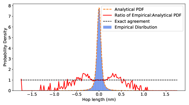
Determining where to truncate the hop distribution: A pure Lévy stable distribution has heavy tails which can lead to arbitrarily long hop lengths. Our distribution of hop lengths fits well to a Lévy distribution near the mean, but under-samples the tails. In Figure 16 we compare the empirically measured transition emission distribution of the MSDDM for urea to its maximum likelihood fit to a Lévy stable distribution. The ratio between the two distributions at each bin is nearly 1 close to the center, indicating a near-perfect fit, larger than 1 slightly further from the center, suggesting that we slightly over sample intermediate hop lengths, and below 1 far from the center, indicating undersampling of extremely long hop lengths. Based on the plot, we chose a cut-off of 1 nm in order to compensate for over sampled intermediate hop lengths. We chose the same cut-off for all solutes.
Generating FLM realizations from a truncated Lévy distribution: To generate realizations from an uncorrelated truncated Lévy process, one would randomly sample from the base distribution and replace values that are too large with new random samples from the base distribution, repeating the process until all samples are under the desired cut-off.
This procedure is complicated by the correlation structure of FLM. At a high level, Stoev and Taqqu use Riemann-sum approximations of the stochastic integrals defining FLM in order to generate realizations. 48 They do this efficiently with the help of Fast Fourier Transforms. In practice, this requires one to Fourier transform a zero-padded vector of random samples drawn from the appropriate Lévy stable distribution, multiply the vector in Fourier space by a kernel function and invert back to real space. The end result is a correlated vector of fractional Lévy noise.
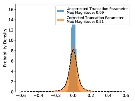
We are unaware of a technique for simulating truncated FLM, therefore we devised our own based on the above discussion. If one is to truncate an FLM process, one can apply the simple procedure above for drawing uncorrelated values from the marginal Lévy stable distribution, but, after adding correlation, the maximum drawn value is typically lower than the limit set by the user. Additionally, the shape of the distribution itself changes. Therefore, we created a database meant to correct the input truncation parameter (the maximum desired draw). The database returns the value of the truncation parameter that will properly truncate the output marginal distribution based on , and (the width parameter). Figure 17(a) shows the result of applying our correction. Note that generating this database requires a significant amount of simulation and still likely doesn’t perfectly correct the truncation parameter. The output leads to a somewhat fuzzy, rather than abrupt, cut-off of the output distribution. This is likely beneficial since we observe a small proportion of hops longer the chosen truncation cut-off. When the cut-off value is close to the Lévy stable parameter, as it is in our anomalous diffusion models, we observed that the tails of the truncated distribution tend to be undersampled. In order to maintain the distribution’s approximate shape up to the cut-off value we recommend ensuring that the cut-off value is at least 2 times . However, this may lead to a slight over-prediction of the MSD.
E.2 Achieving the right correlation structure
We simulated FLM using the algorithm of Stoev and Taqqu 48. There are no known exact methods for simulating FLM. As a consequence, passing a value of and to the algorithm does not necessarily result in the correct correlation structure, although the marginal Lévy stable distribution is correct. We applied a database-based empirical correction in order to use the algorithm to achieve the correct marginal distribution and correlation structure.
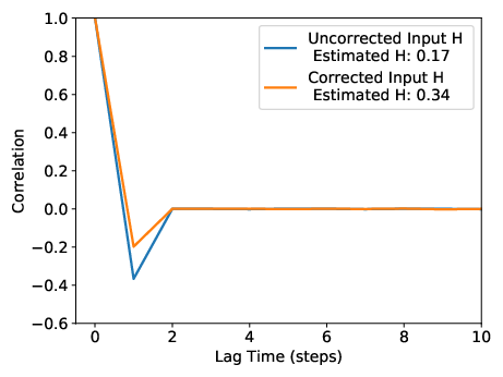
Stoev and Taqqu note that the transition between negatively and positively correlated draws occurs when . When , the marginal distribution is Gaussian and the transition occurs at as expected from FBM. We corrected the input so that the value of measured based on the output sequence equaled the desired . We first adjusted the value of by adding (), effectively recentering the correlation sign transition for any value of . This correction alone does a good job for input values near 0.5, but is insufficient if one desires a low value of . The exact correction to is not obvious so we created a database of output values tabulated as a function of input and values. Figure 17(b) demonstrates the results of applying our correction. Without the correction, FLM realizations are more negatively correlated. This would result in under-predicted mean squared displacements when applying the model.
Appendix F Verifying Markovianity
We verified the Markovianity of our transition matrix, , in two ways. First we ensured that the process satisfied detailed balance:
| (19) |
where is the equilibrium distribution of states. This implies that the number of transitions from state to and from state to should be equal. Graphical representations of the count matrices show that this is true in Figure 18.
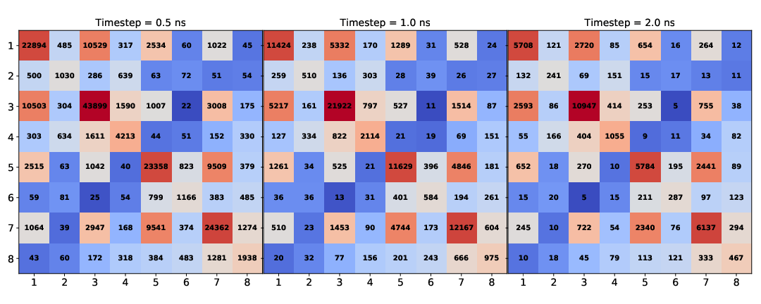
Second, we ensured that the transition matrix did not change on coarser time scales. In Figures 18 and 19, we show that increasing the length of time between samples does not change the properties of the count or probability transition matrices.

Appendix G Derivation of Passage Time Distributions
To derive an analytical equation for the mean first passage time (Equation 9 of the main text), first consider an initial pulse spreading out over time with a fixed mean. We can solve for the time-dependent probability density of particle positions, , by solving the one dimensional diffusion equation:
| (20) |
The appropriate initial and boundary conditions are:
It has been shown elsewhere that the solution to this equation is: 53
| (21) |
We can make the substitution , where represents a constant average velocity, in order to linearly shift the mean as a function of time:
| (22) |
One can track the fraction of particles, , that have crossed the pore boundary by integrating:
| (23) |
where is the pore length. This represents the cumulative first passage time distribution so we take its derivative in order to arrive at the first passage time distribution:
| (24) |
where the only free parameters for fitting are and . We calculated the expected value of Equation 24 in order to get the MFPT. Specifically, we used the python package scipy.integrate.quad to numerically integrate:
| (25) |
Appendix H Solute hopping and trapping behavior
Figure 20 demonstrates that all solutes exhibit the same kind of anti-correlated hopping and trapping behavior.
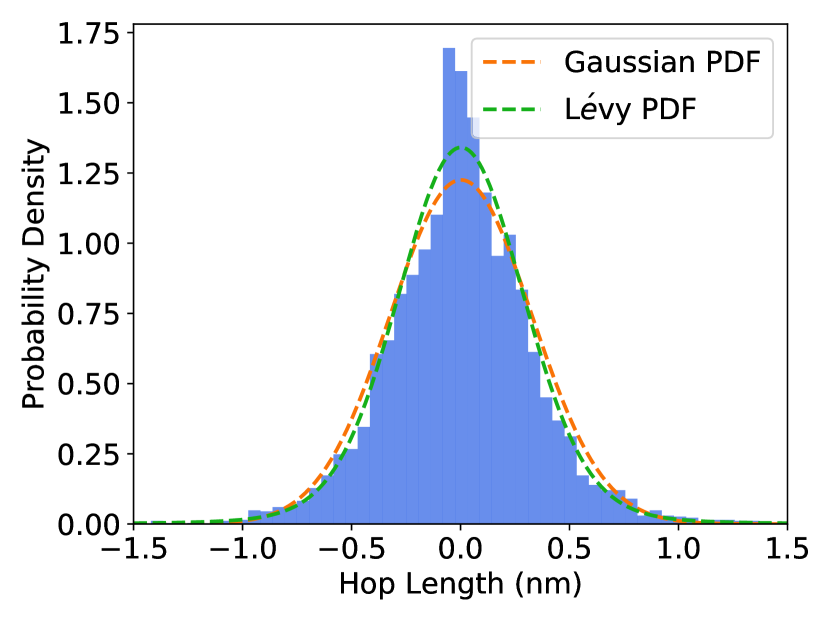
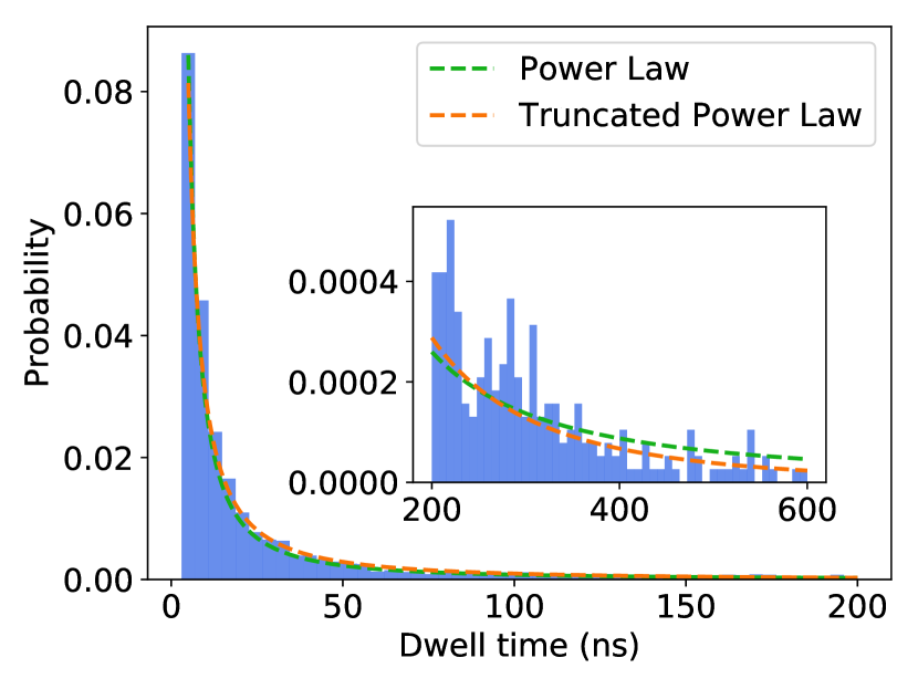
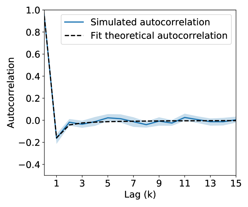
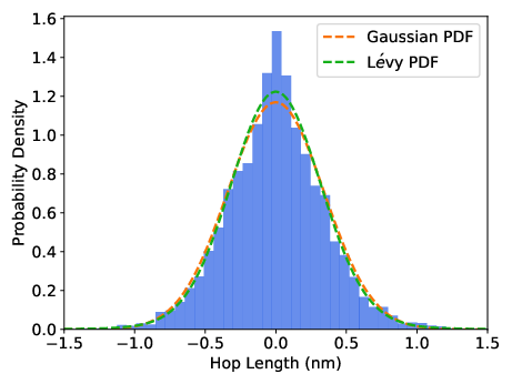

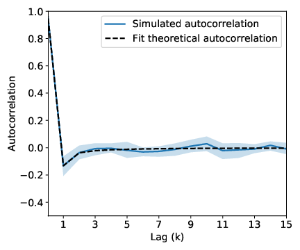
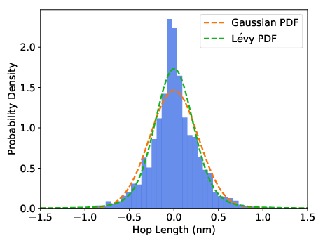
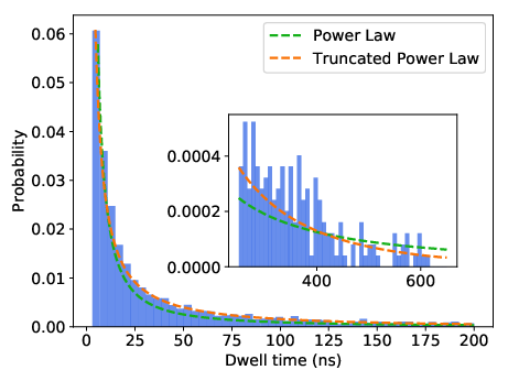
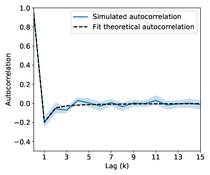
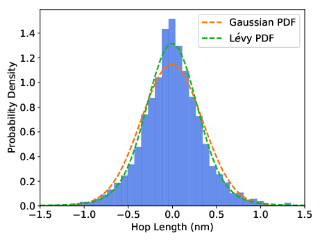
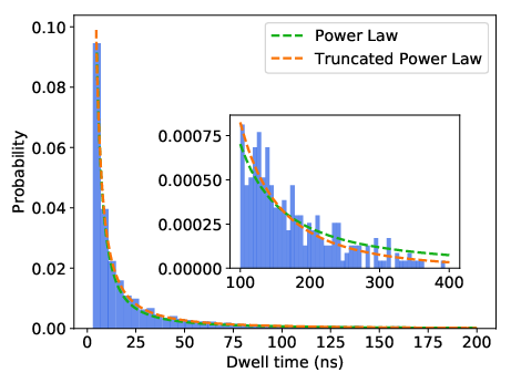
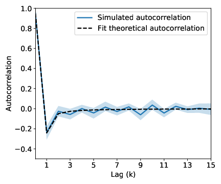
Appendix I AD model MSD Predictions with Pure Power Law Dwell Times
When we use a pure power law distribution to parameterize the dwell time distributions of the one and two mode AD models, the MD MSDs are severely under-predicted because we are incorporating dwell times on the order of the simulation length into simulated trajectories (see Figure 21). The parameters of the pure power law distribution are included in Figure 22.
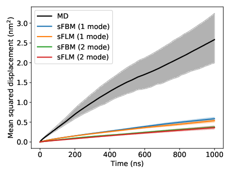
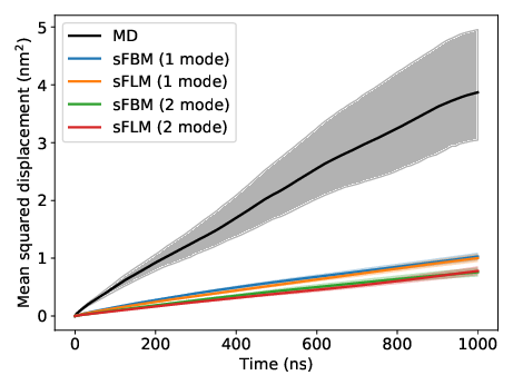
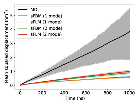
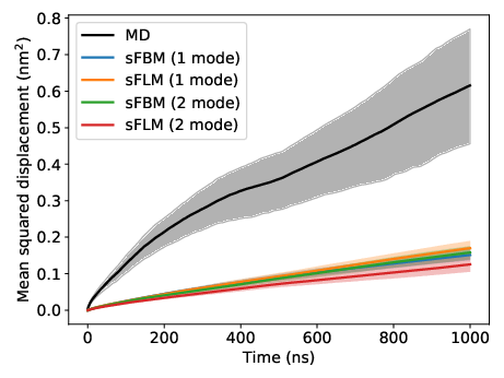

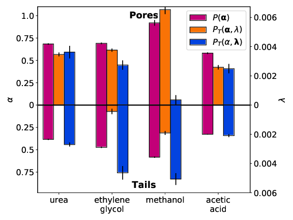
Appendix J Stationarity of Solute Trajectories
We observe that in some cases, solute trajectories extracted from our MD simulations display non-stationary behavior. We defined the perceived equilibration time point for each solute based on the time at which the number of solutes inside the pores and tails stabilized (Figure 14). With this definition, we observe evidence of non-stationary solute behavior after the perceived equilibration point, on the s timescale.
We trained the model parameters on the first half of the equilibrated MD trajectory data and then compared the MSD calculated from AD model realizations to the MSD calculated from the second half of the equilibrated MD trajectory data. This metric is only meaningful if the ensemble of solute trajectories is stationary. In Figure 23, we show that urea and acetic acid show acceptable stationary behavior while methanol and ethylene glycol do not.
We validated both the one and two mode AD models with urea and acetic acid, since their trajectories appear stationary. The MSDs resulting from 1000 realizations of the AD model are shown in Figure 24. We consider the model’s prediction to match well if the MSD lies within the 1 confidence intervals of the MD MSDs. We also look for qualitative agreement in the shape of the curves.
The models are capable of reasonably predicting the MD MSD values of the second half of the solute trajectories based on parameters generated from the first half when the dwell time distributions are parameterized by a power law with an exponential cut-off. At long timescales, the MSD of urea is under-predicted for both the one and two mode models with the same true of acetic acid on short timescales. Without truncation of the power law distribution, the MD MSDs are underestimated in all cases because dwell times on the order of the MD simulation length are sampled and incorporated into the simulated anomalous diffusion trajectories.
This brief analysis suggests that we may be operating on the border of the minimum amount of data required to accurately parameterize AD approach models. Working with only half of the data we collected ( 2 s post-equilibration) may not always be sufficient for extracting reliable parameter estimates. Therefore, in the main text, we employ parameters fit to the entire equilibrated portion of the solute trajectories. Even doubling the data might not be good enough for molecules with statistical non-stationarity, meaning the predictive and interpretive power of the time series modeling applied to these trajectories will be lower.
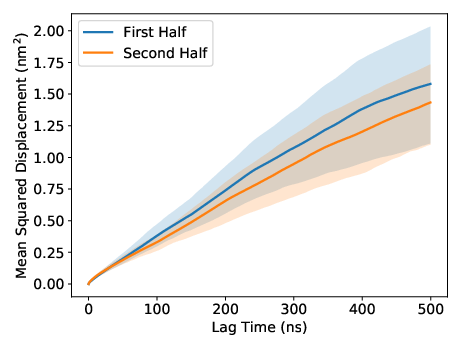
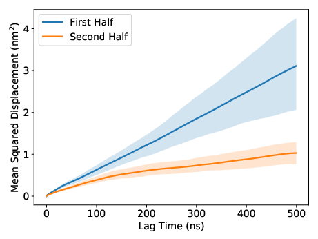

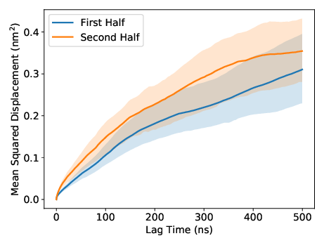
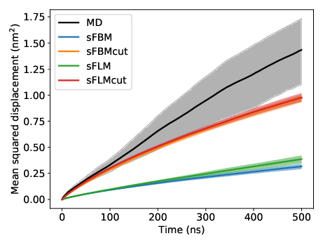
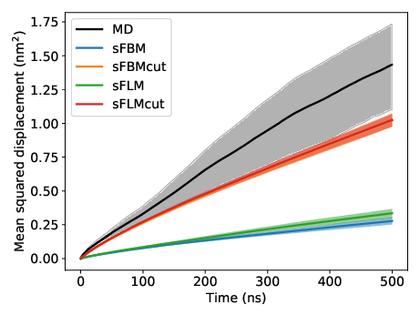
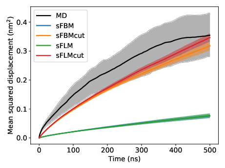

Appendix K Tables of Anomalous Diffusion Parameters
The tables in this section are tabular representations of the parameters depicted in Figures 5 and 6 of the main text and used to generate AD approach realizations whose MSDs are shown in Figure 4 of the main text.
| 1 Mode Model | Parameters | Urea | Ethylene Glycol | Methanol | Acetic Acid |
| Dwell | 0.57 | 0.62 | 0.62 | 0.45 | |
| Distributions | 0.40, 0.0024 | 0.47, 0.0030 | 0.44, 0.0040 | 0.08, 0.0033 | |
| Hop | 0.33 | 0.34 | 0.35 | 0.27 | |
| Distributions | 0.21, 1.84 | 0.23, 1.92 | 0.22, 1.80 | 0.16, 1.72 | |
| Correlation | 0.37 | 0.40 | 0.30 | 0.34 |
| 2 Mode Model | ||||||
|---|---|---|---|---|---|---|
| Parameters | Mode | Urea | Ethylene Glycol | Methanol | Acetic Acid | |
| 1 | 0.69 | 0.69 | 0.90 | 0.58 | ||
| Dwell | 2 | 0.38 | 0.48 | 0.58 | 0.33 | |
| Distributions | 1 | 0.56, 0.0037 | 0.62, 0.0026 | 1.04, 0.0006 | 0.41, 0.0026 | |
| 2 | 0.00, 0.0027 | 0.06, 0.0049 | 0.30, 0.0054 | 0.00, 0.0021 | ||
| 1 | 0.35 | 0.38 | 0.45 | 0.32 | ||
| Hop | 2 | 0.24 | 0.23 | 0.32 | 0.17 | |
| Distributions | 1 | 0.24, 1.91 | 0.26, 1.99 | 0.31, 1.97 | 0.21, 1.91 | |
| 2 | 0.12, 1.50 | 0.15, 1.90 | 0.20, 1.85 | 0.09, 1.50 | ||
| Correlation | – | 0.37 | 0.40 | 0.30 | 0.34 | |
Appendix L MSDDM parameters
We observe correlated emissions drawn from Lévy stable distributions. The deviation of the emission distributions from Gaussian behavior is far more pronounced than that seen in the hop length distributions of the AD model. (see Figure 25(a)) We therefore did not consider the Gaussian case for the MSDDM. The correlation structure between hops is consistent with that of FLM (Figure 25(b)).
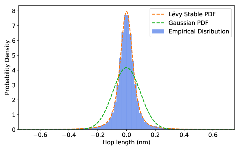
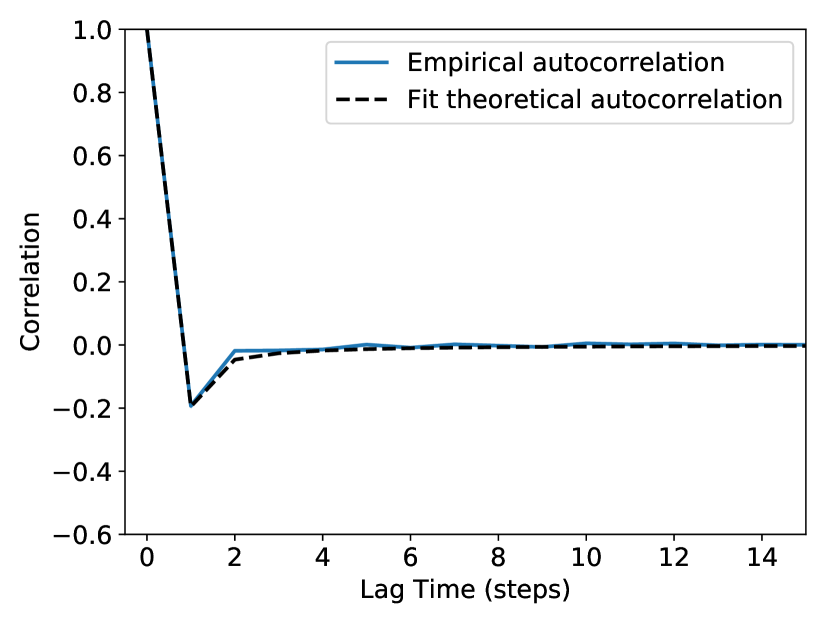
The following table is a tabular representation of the parameters depicted in Figure 8 of the main text.
| Urea | Ethylene Glycol | Methanol | Acetic Acid | |||||||||
|---|---|---|---|---|---|---|---|---|---|---|---|---|
| State | H | H | H | H | ||||||||
| 1 | 0.10 | 1.79 | 0.034 | 0.09 | 1.68 | 0.045 | 0.11 | 1.56 | 0.052 | 0.10 | 1.78 | 0.035 |
| 2 | 0.06 | 1.80 | 0.033 | 0.09 | 1.75 | 0.037 | 0.07 | 1.63 | 0.043 | 0.08 | 1.88 | 0.032 |
| 3 | 0.11 | 1.88 | 0.030 | 0.11 | 1.86 | 0.030 | 0.02 | 1.80 | 0.036 | 0.04 | 2.00 | 0.030 |
| 4 | 0.10 | 1.95 | 0.027 | 0.04 | 1.91 | 0.028 | 0.02 | 1.75 | 0.036 | 0.04 | 2.00 | 0.027 |
| 5 | 0.19 | 1.34 | 0.048 | 0.15 | 1.40 | 0.062 | 0.10 | 1.28 | 0.074 | 0.13 | 1.47 | 0.048 |
| 6 | 0.15 | 1.45 | 0.040 | 0.11 | 1.52 | 0.040 | 0.03 | 1.50 | 0.042 | 0.09 | 1.70 | 0.038 |
| 7 | 0.15 | 1.61 | 0.032 | 0.05 | 1.60 | 0.040 | 0.28 | 1.20 | 0.043 | 0.08 | 1.77 | 0.031 |
| 8 | 0.11 | 1.71 | 0.028 | 0.05 | 1.74 | 0.030 | 0.04 | 1.83 | 0.037 | 0.01 | 2.00 | 0.030 |
| T | 0.34 | 1.42 | 0.036 | 0.37 | 1.44 | 0.045 | 0.35 | 1.45 | 0.057 | 0.34 | 1.54 | 0.040 |
Analytical fits to MFPT distributions
In Figure 26 we demonstrate the high quality of our analytical fits of Equation 24 to the distribution of solute first passage times derived from both the AD and MSDDM models. In Figures 27– 29, we show that one can reliably fit Equation 24 to the passage time distributions with as few as 100 independent trajectory realizations at each pore length. For higher precision, we recommend using at least 1000 trajectories.

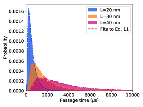
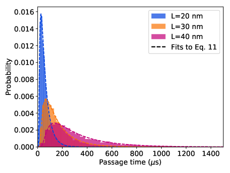
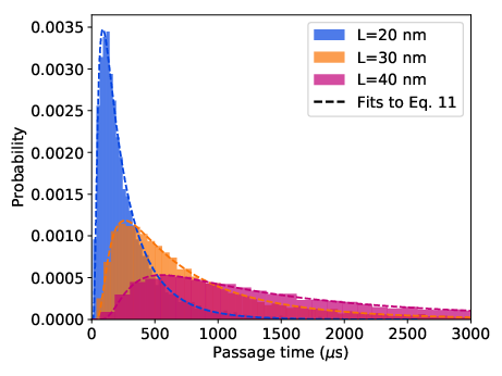
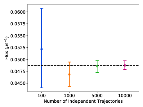
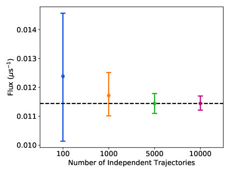

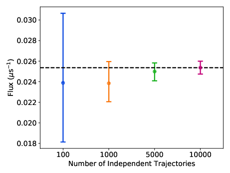
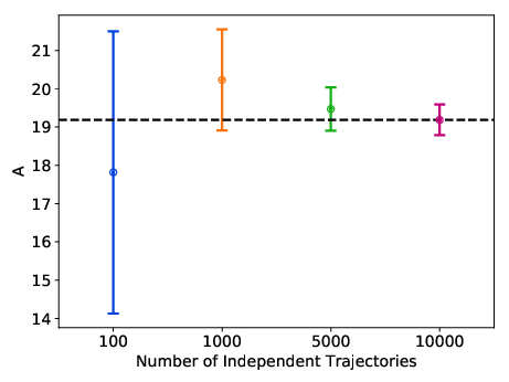
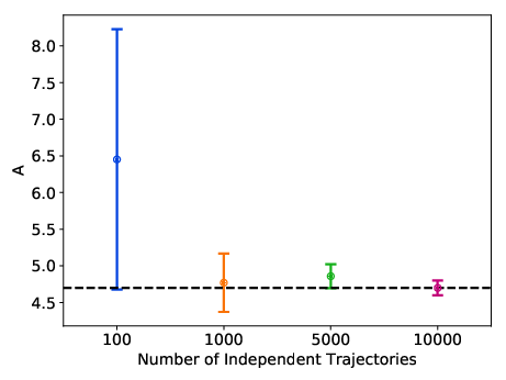
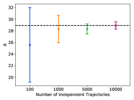
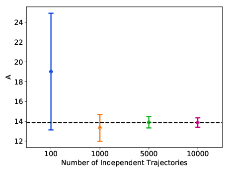
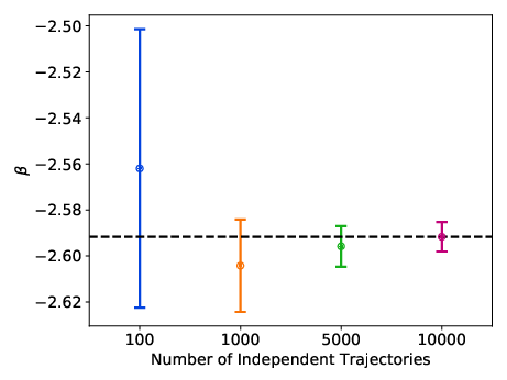
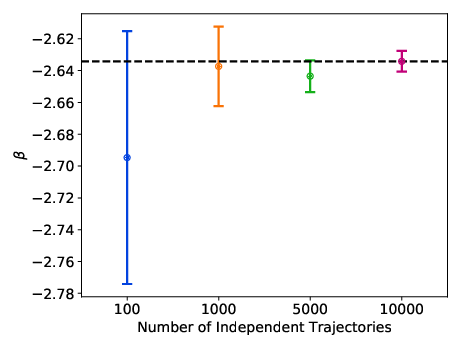
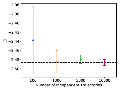
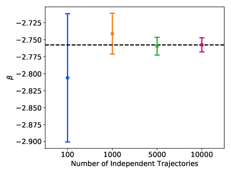
References
- Werber et al. 2016 Werber, J. R.; Osuji, C. O.; Elimelech, M. Materials for Next-Generation Desalination and Water Purification Membranes. Nat. Rev. Mater. 2016, 1, 16018
- Barbosa et al. 2016 Barbosa, M. O.; Moreira, N. F. F.; Ribeiro, A. R.; Pereira, M. F. R.; Silva, A. M. T. Occurrence and Removal of Organic Micropollutants: An Overview of the Watch List of Eu Decision 2015/495. Water Research 2016, 94, 257–279
- Gin et al. 2008 Gin, D. L.; Bara, J. E.; Noble, R. D.; Elliot, B. J. Polymerized Lyotropic Liquid Crystal Assemblies for Membrane Applications. Macromol. Rapid Commun. 2008, 29, 367–389
- Dischinger et al. 2017 Dischinger, S. M.; Rosenblum, J.; Noble, R. D.; Gin, D. L.; Linden, K. G. Application of a Lyotropic Liquid Crystal Nanofiltration Membrane for Hydraulic Fracturing Flowback Water: Selectivity and Implications for Treatment. J. Membr. Sci. 2017, 543, 319–327
- Dischinger et al. 2017 Dischinger, S. M.; McGrath, M. J.; Bourland, K. R.; Noble, R. D.; Gin, D. L. Effect of Post-Polymerization Anion-Exchange on the Rejection of Uncharged Aqueous Solutes in Nanoporous, Ionic, Lyotropic Liquid Crystal Polymer Membranes. J. Membr. Sci. 2017, 529, 72–79
- Feng et al. 2014 Feng, X.; Tousley, M. E.; Cowan, M. G.; Wiesenauer, B. R.; Nejati, S.; Choo, Y.; Noble, R. D.; Elimelech, M.; Gin, D. L.; Osuji, C. O. Scalable Fabrication of Polymer Membranes with Vertically Aligned 1 nm Pores by Magnetic Field Directed Self-Assembly. ACS Nano 2014, 8, 11977–11986
- Feng et al. 2016 Feng, X.; Nejati, S.; Cowan, M. G.; Tousley, M. E.; Wiesenauer, B. R.; Noble, R. D.; Elimelech, M.; Gin, D. L.; Osuji, C. O. Thin Polymer Films with Continuous Vertically Aligned 1 nm Pores Fabricated by Soft Confinement. ACS Nano 2016, 10, 150–158
- Carter et al. 2012 Carter, B. M.; Wiesenauer, B. R.; Hatakeyama, E. S.; Barton, J. L.; Noble, R. D.; Gin, D. L. Glycerol-Based Bicontinuous Cubic Lyotropic Liquid Crystal Monomer System for the Fabrication of Thin-Film Membranes with Uniform Nanopores. Chem. Mater. 2012, 24, 4005–4007
- Hatakeyama et al. 2010 Hatakeyama, E. S.; Wiesenauer, B. R.; Gabriel, C. J.; Noble, R. D.; Gin, D. L. Nanoporous, Bicontinuous Cubic Lyotropic Liquid Crystal Networks via Polymerizable Gemini Ammonium Surfactants. Chem. Mater. 2010, 22, 4525–4527
- Smith et al. 1997 Smith, R. C.; Fischer, W. M.; Gin, D. L. Ordered Poly(p-phenylenevinylene) Matrix Nanocomposites Via Lyotropic Liquid-Crystalline Monomers. J. Am. Chem. Soc. 1997, 119, 4092–4093
- Zhou et al. 2003 Zhou, W.; Gu, W.; Xu, Y.; Pecinovsky, C. S.; Gin, D. L. Assembly of Acidic Amphiphiles into Inverted Hexagonal Phases Using an L-Alanine-Based Surfactant as a Structure-Directing Agent. Langmuir 2003, 19, 6346–6348
- Resel et al. 2000 Resel, R.; Leising, G.; Markart, P.; Kriechbaum, M.; Smith, R.; Gin, D. Structural Properties of Polymerised Lyotropic Liquid Crystals Phases of 3,4,5-Tris(-acryloxyalkoxy)benzoate Salts. Macromol. Chem. Phys. 2000, 201, 1128–1133
- Coscia and Shirts 2019 Coscia, B. J.; Shirts, M. R. Chemically Selective Transport in a Cross-Linked HII Phase Lyotropic Liquid Crystal Membrane. J. Phys. Chem. B 2019,
- Vinh-Thang and Kaliaguine 2013 Vinh-Thang, H.; Kaliaguine, S. Predictive Models for Mixed-Matrix Membrane Performance: A Review. Chem. Rev. 2013, 113, 4980–5028
- Geens et al. 2006 Geens, J.; Van der Bruggen, B.; Vandecasteele, C. Transport Model for Solvent Permeation Through Nanofiltration Membranes. Sep. Purif. Technol. 2006, 48, 255–263
- Darvishmanesh and Van der Bruggen 2016 Darvishmanesh, S.; Van der Bruggen, B. Mass Transport through Nanostructured Membranes: Towards a Predictive Tool. Membranes 2016, 6
- Wijmans and Baker 1995 Wijmans, J. G.; Baker, R. W. The Solution-Diffusion Model: A Review. J. Membr. Sci. 1995, 107, 1–21
- Paul 1974 Paul, D. R. In Permeability of Plastic Films and Coatings: To Gases, Vapors, and Liquids; Hopfenberg, H. B., Ed.; Polymer Science and Technology; Springer US: Boston, MA, 1974; pp 35–48
- Manzo and Garcia-Parajo 2015 Manzo, C.; Garcia-Parajo, M. F. A Review of Progress in Single Particle Tracking: From Methods to Biophysical Insights. Rep. Prog. Phys. 2015, 78, 124601
- Maginn et al. 2018 Maginn, E. J.; Messerly, R. A.; Carlson, D. J.; Roe, D. R.; Elliott, J. R. Best Practices for Computing Transport Properties 1. Self-Diffusivity and Viscosity from Equilibrium Molecular Dynamics [article V1.0]. LiveCoMS 2018, 1, 6324
- Metzler and Klafter 2000 Metzler, R.; Klafter, J. The Random Walk’s Guide to Anomalous Diffusion: A Fractional Dynamics Approach. Phys. Rep. 2000, 339, 1–77
- Bouchaud and Georges 1990 Bouchaud, J.-P.; Georges, A. Anomalous Diffusion in Disordered Media: Statistical Mechanisms, Models and Physical Applications. Phys. Rep. 1990, 195, 127–293
- Gorenflo and Mainardi 1997 Gorenflo, R.; Mainardi, F. In Fractals and Fractional Calculus in Continuum Mechanics; Carpinteri, A., Mainardi, F., Eds.; International Centre for Mechanical Sciences; Springer Vienna: Vienna, 1997; pp 223–276
- Klages et al. 2008 Klages, R.; Radons, G.; Sokolov, I. M. Anomalous Transport: Foundations and Applications; John Wiley & Sons, 2008; Google-Books-ID: TDch5DfNgWoC
- Mandelbrot and Van Ness 1968 Mandelbrot, B.; Van Ness, J. Fractional Brownian Motions, Fractional Noises and Applications. SIAM Rev. 1968, 10, 422–437
- Jeon and Metzler 2010 Jeon, J.-H.; Metzler, R. Fractional Brownian Motion and Motion Governed by the Fractional Langevin Equation in Confined Geometries. Phys. Rev. E 2010, 81, 021103
- Banks and Fradin 2005 Banks, D. S.; Fradin, C. Anomalous Diffusion of Proteins Due to Molecular Crowding. Biophys. J. 2005, 89, 2960–2971
- Montroll and Weiss 1965 Montroll, E. W.; Weiss, G. H. Random Walks on Lattices. II. J. Math. Phys. 1965, 6, 167–181
- Snow et al. 2005 Snow, C. D.; Sorin, E. J.; Rhee, Y. M.; Pande, V. S. How Well Can Simulation Predict Protein Folding Kinetics and Thermodynamics? Annu. Rev. Biophys. Biomol. Struct. 2005, 34, 43–69
- Chodera et al. 2007 Chodera, J. D.; Singhal, N.; Pande, V. S.; Dill, K. A.; Swope, W. C. Automatic Discovery of Metastable States for the Construction of Markov Models of Macromolecular Conformational Dynamics. J. Chem. Phys. 2007, 126, 155101
- Chodera and Noé 2014 Chodera, J. D.; Noé, F. Markov State Models of Biomolecular Conformational Dynamics. Curr. Opin. Struct. Biol. 2014, 25, 135–144
- Bowman et al. 2009 Bowman, G. R.; Huang, X.; Pande, V. S. Using Generalized Ensemble Simulations and Markov State Models to Identify Conformational States. Methods 2009, 49, 197–201
- Bekker et al. 1993 Bekker, H.; Berendsen, H. J. C.; Dijkstra, E. J.; Achterop, S.; van Drunen, R.; van der Spoel, D.; Sijbers, A.; Keegstra, H.; Reitsma, B.; Renardus, M. K. R. GROMACS: A Parallel Computer for Molecular Dynamics Simulations; Physics Computing ’92: Proceedings of the 4th International Conference, Praha, Czechoslovakia, Aug 24-28, 1992; World Scientific: Singapore, 1993
- Berendsen et al. 1995 Berendsen, H. J. C.; van der Spoel, D.; van Drunen, R. GROMACS: A Message-Passing Parallel Molecular Dynamics Implementation. Comput. Phys. Commun. 1995, 91, 43–56
- Van Der Spoel et al. 2005 Van Der Spoel, D.; Lindahl, E.; Hess, B.; Groenhof, G.; Mark, A. E.; Berendsen, H. J. C. GROMACS: Fast, Flexible, and Free. J. Comput. Chem. 2005, 26, 1701–1718
- Hess et al. 2008 Hess, B.; Kutzner, C.; van der Spoel, D.; Lindahl, E. GROMACS 4: Algorithms for Highly Efficient, Load-Balanced, and Scalable Molecular Simulation. J. Chem. Theory Comput. 2008, 4, 435–447
- Truong et al. 2018 Truong, C.; Oudre, L.; Vayatis, N. Ruptures: Change Point Detection in Python. arXiv 2018, arXiv:1801.00826
- Meroz and Sokolov 2015 Meroz, Y.; Sokolov, I. M. A Toolbox for Determining Subdiffusive Mechanisms. Phys. Rep. 2015, 573, 1–29
- Clauset et al. 2009 Clauset, A.; Shalizi, C.; Newman, M. Power-Law Distributions in Empirical Data. SIAM Rev. 2009, 51, 661–703
- Newman 2005 Newman, M. E. J. Power Laws, Pareto Distributions and Zipf’s Law. Contemp. Phys. 2005, 46, 323–351
- Metzler et al. 2014 Metzler, R.; Jeon, J.-H.; Cherstvy, A. G.; Barkai, E. Anomalous Diffusion Models and Their Properties: Non-Stationarity, Non-Ergodicity, and Ageing at the Centenary of Single Particle Tracking. Phys. Chem. Chem. Phys. 2014, 16, 24128–24164
- Neusius et al. 2009 Neusius, T.; Sokolov, I. M.; Smith, J. C. Subdiffusion in Time-Averaged, Confined Random Walks. Phys. Rev. E 2009, 80, 011109
- Tikanmäki and Mishura 2010 Tikanmäki, H.; Mishura, Y. Fractional Lévy Processes as a Result of Compact Interval Integral Transformation. arXiv:1002.0780 [math] 2010, arXiv: 1002.0780
- Bishwal 2011 Bishwal, J. P. N. Maximum Quasi-likelihood Estimation in Fractional Levy Stochastic Volatility Model. JMF 2011, 01, 58–62
- Mantegna and Stanley 1994 Mantegna, R. N.; Stanley, H. E. Stochastic Process with Ultraslow Convergence to a Gaussian: The Truncated Lévy Flight. Phys. Rev. Lett. 1994, 73, 2946–2949
- Bacallado et al. 2009 Bacallado, S.; Chodera, J. D.; Pande, V. Bayesian Comparison of Markov Models of Molecular Dynamics with Detailed Balance Constraint. J. Chem. Phys. 2009, 131, 045106
- Flynn 2019 Flynn, C. R. Exact Methods for Simulating Fractional Brownian Motion and Fractional Gaussian Noise in Python. 2019; \urlhttps://github.com/crflynn/fbm
- Stoev and Taqqu 2004 Stoev, S.; Taqqu, M. S. Simulation Methods for Linear Fractional Stable Motion and Farima Using the Fast Fourier Transform. Fractals 2004, 12, 95–121
- Pande et al. 2010 Pande, V. S.; Beauchamp, K.; Bowman, G. R. Everything You Wanted to Know About Markov State Models but Were Afraid to Ask. Methods 2010, 52, 99–105
- Wehmeyer et al. 2018 Wehmeyer, C.; Scherer, M. K.; Hempel, T.; Husic, B. E.; Olsson, S.; Noé, F. Introduction to Markov State Modeling with the Pyemma Software [article V1.0]. LiveCoMS 2018, 1, 5965–
- Luzar and Chandler 1996 Luzar, A.; Chandler, D. Effect of Environment on Hydrogen Bond Dynamics in Liquid Water. Phys. Rev. Lett. 1996, 76, 928–931
- Hill 1989 Hill, T. L. Free Energy Transduction and Biochemical Cycle Kinetics; Springer-Verlag, 1989
- Cussler 2009 Cussler, E. L. Diffusion: Mass Transfer in Fluid Systems, 3rd ed.; Cambridge University Press, 2009
- Guo et al. 2004 Guo, W. F.; Chung, T.-S.; Matsuura, T. Pervaporation Study on the Dehydration of Aqueous Butanol Solutions: A Comparison of Flux Vs. Permeance, Separation Factor Vs. Selectivity. J. Membr. Sci. 2004, 245, 199–210
- Kedem and Katchalsky 1963 Kedem, O.; Katchalsky, A. Permeability of Composite Membranes. Part 1.—Electric Current, Volume Flow and Flow of Solute Through Membranes. Trans. Faraday Soc. 1963, 59, 1918–1930
- Al-Zoubi et al. 2007 Al-Zoubi, H.; Hilal, N.; Darwish, N. A.; Mohammad, A. W. Rejection and Modelling of Sulphate and Potassium Salts by Nanofiltration Membranes: Neural Network and Spiegler–Kedem Model. Desalination 2007, 206, 42–60
- Ernst et al. 2012 Ernst, D.; Hellmann, M.; Köhler, J.; Weiss, M. Fractional Brownian Motion in Crowded Fluids. Soft Matter 2012, 8, 4886–4889
- Bel and Barkai 2005 Bel, G.; Barkai, E. Weak Ergodicity Breaking in the Continuous-Time Random Walk. Phys. Rev. Lett. 2005, 94, 240602
- Clegg 2006 Clegg, R. G. A Practical Guide to Measuring the Hurst Parameter. arXiv:math/0610756 2006, arXiv: math/0610756