History matching with probabilistic emulators and active learning

Abstract

The scientific understanding of real-world processes has dramatically improved over the years through computer simulations. Such simulators represent complex mathematical models that are implemented as computer codes which are often expensive. The validity of using a particular simulator to draw accurate conclusions relies on the assumption that the computer code is correctly calibrated. This calibration procedure is often pursued under extensive experimentation and comparison with data from a real-world process. The problem is that the data collection may be so expensive that only a handful of experiments are feasible. History matching is a calibration technique that, given a simulator, it iteratively discards regions of the input space using an implausibility measure. When the simulator is computationally expensive, an emulator is used to explore the input space. In this paper, a Gaussian process provides a complete probabilistic output that is incorporated into the implausibility measure. The identification of regions of interest is accomplished with recently developed annealing sampling techniques. Active learning functions are incorporated into the history matching procedure to refocus on the input space and improve the emulator. The efficiency of the proposed framework is tested in well-known examples from the history matching literature, as well as in a proposed testbed of functions of higher dimensions.

1 Introduction

Computer simulations have played an essential role in vastly improving our understanding of real-world processes. These computational models are parameterised by a set of values which determine the behaviour of the simulator and its ability to replicate the process under consideration. No matter how sophisticated or efficient, a simulator must be well-calibrated to experimental data if it is to be trusted. Thus, the validity of using a particular simulator to draw accurate conclusions, relies on the assumption that the model has been correctly calibrated. That is, the vector of input parameters is well known, and there is confidence that these values are able to replicate the process the simulator is modeling. This calibration procedure is often pursued under extensive code experimentation guided by expert domain knowledge.

Successful model calibration is achieved with data collected from measurements of the phenomenon under study. For some models, the collection of data can be so expensive that only a handful of experiments is feasible. This is common in applications such as astrophysics [47], epidemiology [1], and climate modeling [40], to name a few. History matching [3, 47] is a calibration technique that iteratively discards regions of the input space through the use of an implausibility measure. This way, history matching overcomes the limited availability of experimental data (measurements) and is able to identify regions of input space that are likely to replicate the observed phenomenon, given different sources of uncertainty. Thus, the regions that show high implausibility can be discarded from the analysis. Furthemore, history matching is also able to determine whether there is no region of interest, that is, no combination of input values that is likely to match the available data. This can be used as evidence that further improvement in the simulator is needed. This contrasts with typical Bayesian analysis of computer code output (BACCO, [30]) where positive posterior probability mass is always assigned to regions that under the history matching framework would otherwise be discarded.

Increasing complexity in mathematical models often translates in increasing computational cost of the corresponding simulator. Thus, the ability to exploit the simulator is limited by computational budget or time constraints. For example, certain simulators used for climate models, nuclear reactor models, and biological models need days to complete a single simulation run [41]. This represents an additional layer of complexity, since the ability to explore the input space is hindered by the high computational cost. Common techniques such as Monte Carlo simulation and its variants are not well suited in this context. In turn, fast but accurate emulators are needed to overcome this limitation. In particular, Gaussian Process (GP) models have been successfully used as Bayesian emulators in different scientific applications such as machine learning [39], spatial data analysis [14], genetics [29], and stochastic finite element analysis [15], to name a few. Since a GP provides a full probabilistic characterisation of the unknown model output, its posterior predictive mean provides a surrogate model, whilst its posterior predictive variance measures the accuracy of the emulator.

The use of simulators and emulators introduces a wide range of uncertainties in the modeling process. In history matching, these uncertainties are elicited and incorporated in the variability of the predicted output [13, 46]. The implausibility measure is defined as a function of the number of expected standard deviations between the observed data and the corresponding emulator output [1]. In the literature, it is common to use the mean of the emulator as an estimate within the implausibility measure to guide the iterative selection of points in the non-implausible domain [13, 46, 49]. This is achieved by computing the absolute value of the difference between the emulator averaged prediction and the experimental data, standardised by different sources of uncertainty. To the authors’ knowledge, using the full probabilistic characterisation of the emulator has not been explored for history matching applications.

In contrast, within the area of robust optimisation of black-box computer codes [28], the probabilistic output of a GP is acknowledged and incorporated in the exploration of the input space through the use of appropriate acquisition functions [19, 38] . The optimisation is performed as an iterative procedure that uses a GP model as an emulator for the black box function [28]. In these applications, the acquisition functions incorporate the probabilistic information from the emulator and is used in turn to guide the exploration of the input space. For instance, the commonly used criterion of expected improvement is guaranteed to find the optima of a function under certain regularity conditions [45]. As a consequence, expected improvement is often preferred to deterministic estimates of improvement to guide the exploration of the input space [19]. This is because the expectation operator considers the uncertainty modeled through the emulator, as opposed to using maximum likelihood (MLE) or maximum a posteriori (MAP) estimate. Motivated by this analogy, the history matching strategy developed in this paper uses a full probabilistic characterisation of the output of the simulator to be able to guide the reduction of the input space at every iteration.

As mentioned before, history matching is a sequential procedure that identifies regions of non-implausible input configurations in order to refocus the emulation of the simulator. Refocusing enables a better identification of non-implausible points by using an improved emulator in the regions of interest. This raises the question of how to choose new simulator runs to improve the current emulator. In this paper, different functions to guide the selection of points are tested. These functions are known in other research communities under the name of active learning criteria [18], sampling criteria [6] and learning functions [34]. In this work, the term active learning is used in order to facilitate a link between the machine learning and history matching communities. Moreover, the term active learning is retained as these criteria guide the identification of regions where the limited computational resources must be spent in light of the evidence of data and observed response from the simulator.

This paper proposes the use of a full probabilistic characterisation of the emulator within the implausibility measure to guide refocusing. In particular, three active learning criteria are generalised and presented as choices to guide the selection of new training runs to iteratively improve the emulator. Firstly, the expected contour improvement [38] is used as it was specially designed to refine an emulator for a given contour level. Secondly, the expected risk [17] used for reliability analysis is modified here to adapt to contour estimation. Thirdly, the entropic profile presented in [34] is also modified to target a specific contour level of an emulator.

The paper is organised as follows. In Section 2 the preliminaries for history matching are presented, with a brief overview of GP emulators. In Section 3 the identification of non-implausible regions is discussed within the context of the simulated annealing sampling methods used in subset optimisation. This provides regions of input parameter space that are likely to match the simulator output to observed data. In Section 4 the proposed active learning criteria are presented. In Section 5 some illustrative examples are shown. Concluding remarks are presented in Section 6.

2 History matching

History matching is a calibration technique particularly useful in settings where not only the model is computationally expensive, but the data-generating process is expensive as well. The seminal papers [12] and [13] introduced history matching within the framework of Bayes linear statistics to analyse computationally expensive computer models. Vernon et al. [46] presented a thorough exposition of history matching in large-scale high-dimensional applications such as the ones encountered in cosmology. A more recent discussion of the history matching framework can be found in [22].

In particular, this paper focuses on the application of history matching in cases where the cost of generating new experimental data is so high that very limited information from the physical process under study can be recorded. In this setting, history matching aims to identify regions of the input parameter space $\mathcal{X}$ of the simulator that are able to replicate the measured data, given the structure of the model and the sources of uncertainty. This corresponds to a relaxation of the search for a single optimal calibration point $\mathbf{x}^{*}$, that matches the simulator output to the physical process. This relaxation consider regions of parameter space that are able to replicate the observed process within a certain level of modeled uncertainty. The more stringent alternative is the typical calibration setting where the objective is to find the unique optimal configuration [4, 44, 30].  In the typical Bayesian alternative one would treat $\mathbf{x}^{*}$ as an unknown parameter, and the posterior distribution for $\mathbf{x}^{*}$ would result from updating the prior specification given some measurements from the physical process. However, it could be the case that there is not enough information to believe that there is a unique choice for $\mathbf{x}^{*}$. There might be doubts in one or several aspects of the specified model. This could mean, for example, that the discrepancy between the model and the phenomenon under study – its structure and independence from an optimal $\mathbf{x}^{*}$ – is not very well understood. These doubts make the interpretation of $\mathbf{x}^{*}$ as the optimal calibration value meaningless.  In this setting, history matching identifies collections of simulator evaluations that are consistent with the measured data within the levels of uncertainty associated with the problem.

The overall strategy of history matching is to use an emulator to explore the input space in order to find regions on which the simulator gives acceptable matches to the data. History matching then discards regions of input space (even in cases where the simulator has a multi-dimensional output) in stages or waves, as introduced in [46]. Thus, history matching sequentially removes regions of parameter space using an implausibility measure. The input regions that are considered non-implausible are sampled to refocus the emulator for the next wave and, as a consequence, further reduce the non-implausible region. The procedure of resampling, re-emulating, and reducing the non-implausible space is done until a stopping condition is met. It should be noted that the history matching process seeks to discard regions where poor matches between simulator output and measurements. This can be done using only a subset of outputs and observations, unlike other approaches which require consideration of all simulator output coordinates.

For the purpose of this paper, let $y$ denote the true physical process of interest. Due to experimental error, $y$ cannot be observed directly. Let $z$ denote the noisy version of the process. That is, $z=y+\epsilon_{\text{me}}$, where $\epsilon_{\text{me}}$ denotes an observational noise with zero mean and finite variance. The limitation of not being able to observe directly the data is what is commonly referred to as observation uncertainty or measurement error. The quantity of interest, $y$, is assumed to be the output of the simulator being calibrated. Let $f(\mathbf{x})$ denote the simulator output using the input parameter $\mathbf{x}\in\mathcal{X}\subset\mathbb{R}^{d}$. The simulator $f(\cdot)$ is assumed to be only a mathematical abstraction of the true underlying process, which adds an additional layer of uncertainty in the computer output. The inevitable mismatch between the computer model and the process is called model discrepancy as in [30]. Some sources of model discrepancy are: reduced accuracy due to floating point arithmetic, simplifying assumptions of the computational model, lack of understanding of the underlying physics, among others. Let $\epsilon_{\text{md}}$ denote the model discrepancy and assume $y=f(\mathbf{x}^{*})+\epsilon_{\text{md}}$, where $\mathbf{x}^{*}$ is the optimal calibration point. Note that model discrepancy can be inferred simultaneously whilst performing calibration, as it is done in the framework described by Kennedy and O’Hagan [30]. However, due to the confounding between $\mathbf{x}^{*}$ and the discrepancy term, it has proven useful to infer first an appropriate calibrated emulator and then model the discrepancy from the residuals. This is called modularized Bayesian inference of computer code output [33, 7]. In histroy matching, however, this discrepancy is usually elicited from domain expert knowledge [2].

As stated before, the computational complexity of the simulator inhibits the ability to explore the configuration space. In typical industrial applications, each run of the simulator could take as much as days or weeks to complete. As a consequence, an additional layer of uncertainty is introduced. In the literature, this is known as code uncertainty. An inexpensive approximation for the simulator is used to cope with this limitation. In this work, the emulator used for the simulator is a full Bayesian GP. The use of a full Bayesian GP provides two advantages in history matching applications. Firstly, uncertainty in the surrogate itself is partially mitigated due to the marginalisation of the GP hyperparameters. Secondly, as a by-product of GP emulators, code uncertainty can be directly estimated due to the analytical expression for the output variability.

A GP is a nonparametric model used for Bayesian inference in function spaces. A GP emulator considers the mapping from input space $\mathcal{X}$ to output $y$ as a stochastic process indexed by $\mathcal{X}$. An intuitive way of thinking of a GP is to view it as an infinite-dimensional extension of a multivariate Gaussian distribution. Just as its finite dimensional counterpart, it is completely determined by its mean function $m(\cdot)$ and covariance kernel $k(\cdot,\cdot)$, which specify its first two moments. The mean function $m(\cdot)$ embodies the understanding of any global trend exhibited by the true process. The covariance kernel, on the other hand, incorporates prior knowledge of any assumptions on how similar input configurations $\mathbf{x},\mathbf{x}^{\prime}\in\mathcal{X}$ produce correlated outputs. An additional property of GP emulators is that the model produces its own measurement of variability, commonly used as predicted error. GP emulators have become standard tools to quantify uncertainty in expensive computer models. For more detail on their theoretical underpinnings and implementation, the interested reader is referred to [39, 36].

Let $\sigma(\mathbf{x})^{2}=k(\mathbf{x},\mathbf{x})$ denote the variability of predicted code output at configuration $\mathbf{x}$. In order to perform Bayesian inference for the GP, the mean and covariance functions have to be chosen beforehand from a family of possible choices [39]. It is common to specify a zero mean process with a squared exponential kernel, which for simplicity is done in this paper. This choice corresponds to a GP that can be interpreted as a radial basis expansion on the locations of the training data. This covariance kernel assumes the emulated function to be infinitely differentiable. Note that elicitation of an appropriate mean function and covariance kernel can be done in such a way that it incorporates domain expert knowledge on expected behaviour of the simulator [35, 46]. The mean and covariance functions are further parameterised by its respective vectors of hyperparameters. These hyperparameters are often selected by an empirical Bayes approach. However in this paper, a fully Bayesian procedure is used in order to acknowledge the limited number of simulator runs available. More details are given below.

Let $\mathcal{D}=\{(\mathbf{x}_{i},y_{i})\}_{i=1}^{N}$ be the collection of input–output pairs used to train the GP emulator. This collection of points is usually chosen so that the input configuration space is explored uniformly in every dimension. A Latin Hypercube Sampling (LHS) scheme is usually chosen to this end. Bayesian inference incorporates prior knowledge on the hyperparameters of the GP, if available, and allows one to compute the posterior distribution given the observed training data. Given the training runs and a Gaussian measurement model for $\epsilon_{\text{me}}$, it can be shown that the posterior prediction on an unseen input configuration $\mathbf{x}^{*}$ follows a Gaussian distribution with posterior mean and covariance functions given by

$$m(\mathbf{x}^{*}) =\sum_{i=1}^{N}w_{i}\,\,m_{i}(\mathbf{x}^{*}),\textbf{}$$ (2.1)

$$\text{cov}(\mathbf{x}^{*},\mathbf{x}^{\prime}) =\sum_{i=1}^{N}w_{i}\,\,\left[(m_{i}(\mathbf{x}^{*})-m(\mathbf{x}^{*}))(m_{i}(\mathbf{x}^{\prime})-m(\mathbf{x}^{\prime}))+\text{cov}_{i}(\mathbf{x}^{*},\mathbf{x}^{\prime})\right],$$ (2.2)

where $m_{i}(\mathbf{x}^{*})$ and $\text{cov}_{i}(\mathbf{x}^{*},\mathbf{x}^{\prime})$ denote the posterior mean and covariance functions of the GP emulator with hyperparameter vector $\boldsymbol{\theta}_{i}$. The sum denotes a Monte Carlo approximation to the integral with respect to the posterior distribution $p(\boldsymbol{\theta}|\mathcal{D})$ with corresponding weights $w_{i}$. Note that $\text{cov}(\mathbf{x}^{*},\mathbf{x}^{*})=\sigma^{2}(x^{*})$ denotes the predicted variance of the GP prediction marginalised by samples of the posterior distribution of the hyperparameters. For a more detailed explanation, the interested reader is referred to [21] and [39].

Let $I(\mathbf{x})$ denote the implausibility measure of the input configuration $\mathbf{x}$ given the observed datum $z$. This implausibility is defined as

$$I(\mathbf{x})=\frac{\Big{|}z-m(x)\Big{|}}{\sqrt{\sigma^{2}(\mathbf{x})+\sigma^{2}_{\text{md}}+\sigma^{2}_{\text{me}}}},$$ (2.3)

where $m(x)$ and $\sigma^{2}(x)$ denote, respectively, the posterior mean and posterior variance of the GP emulator as defined above. It is important to note that, in certain applications, the simulator output is known to be stochastic and an additional term is added in the denominator to account for ensemble variability [1]. In this work such variability is not needed. Furthermore, note that the distance between the data threshold $z$ and the surrogate output is standardised by the sum of the modeled uncertainties. The implausibility function helps identify which configuration points are far from the target, as measured by a number of standard deviations. In the literature, Pukelsheim’s three sigma rule [37] is a common choice to characterise the number of standard deviations in this setting. The rule states that if $X$ is a continuous random variable with mean $m$ and variance $\sigma^{2}$ which follows a uni-modal distribution, then the probability for $X$ falling away from its mean by more than 3 standard deviations is at most 5%. That is,

$$P\{|X-m|>3\,\sigma\}<0.05$$ (2.4)

Following the above criteria, the region of input space where the emulator should refocus is then defined as

$$\mathcal{X}_{\text{NROY}}=\{\mathbf{x}\in\mathcal{X}\,:\,I(\mathbf{x})\leq k\},$$ (2.5)

where $k=3$ following the above considerations, and the subscript stands for Not-ruled-out-yet (NROY) [47].

2.1 History matching with probabilistic emulators

The previous description of history matching stems from the construction of probability by using mathematical expectation as a primitive. This approach is known as Bayes linear statistics, since linearity of expectations is a key aspect in the development of tools under the theory. For a more thorough discussion on Bayesian linear methods refer to [23]. The construction of the implausibility measure under Bayes linear can be seen as a function that uses a pointwise estimate from the emulator. Nonetheless, the GP emulator provides a probabilistic generator of surrogate models, which can be exploited in a full probabilistic formulation. As discussed above, a full probabilistic approach is proposed in this paper, whereby both the GP probabilistic output and the posterior distribution of the hyperparameters are considered for the emulator.

In the proposed characterisation, a full probabilistic treatment of the emulator is used within the implausibility function. This is achieved by incorporating the probabilistic distribution of the GP emulator output. Let the emulated implausibility be defined as

$$I_{\textsf{GP}}(\mathbf{x})=\frac{|z-f_{\textsf{GP}}(\mathbf{x})|}{\sqrt{\sigma^{2}(x)+\sigma^{2}_{\text{md}}+\sigma^{2}_{\text{me}}}},$$ (2.6)

where $f_{\textsf{GP}}(\mathbf{x})\sim\mathsf{N}(m(\mathbf{x}),\sigma^{2}(\mathbf{x}))$ is the GP emulator for the simulator output. The dependence on the training runs $\mathcal{D}$ is omitted to avoid cluttered notation. The NROY space is thus characterised by probabilistic statements of the form

$$P\{I_{\textsf{GP}}(\mathbf{x})\leq 3\},$$ (2.7)

which is analogous to the probabilistic statements of [27] and [51].

The difference between using (2.3) and (2.6) is depicted in Figure 1. The underlying model is the modified Branin function [19], for which a GP emulator is fitted using the blue dots as training points. Dashed lines correspond to the emulator’s response at the target level $z=10$, whilst solid lines correspond to the target level of the Branin function. In both subfigures, the dark-shaded regions correspond to higher values of implausibility, whereas light-shaded regions account for lower values. The contour levels correspond to the number of standard deviations away from the target level $z$. Pitch-black regions in Figure 1(a) indicate values of the implausibility function of $3$ and decrease one unit at a time as the colour becomes white. In Figure 1(b), the levels are chosen logarithmically so that the pitch-black level corresponds to the region of more than $99\%$ probability. This is dictated by the emulator predictive distribution. The rest of the contour levels in Figure 1(b) decrease to levels $90\%$ and $67\%$.

The stochastic nature of the emulator motivates the direct description of implausibility in terms of probabilities. This formulation naturally incorporates the variability from the emulator, which is highly convenient for computationally expensive simulators. In this kind of setting, only a small amount of training data is available, and thus a fully Bayesian approach to emulation might be desired. The dichotomy of selecting new simulator runs close to the emulator response contour level or where there is high uncertainty, is known as the exploration-exploitation trade-off in computer experimental design [19].  Exploration is desirable as the use of an emulator might induce bias if followed too blindly in the first steps of the procedure.

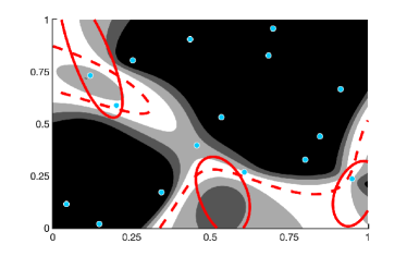
(a) Implausibility measure based on a deterministic emulator.

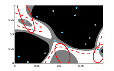
(b) Probability of implausibility based on stochastic emulator.

Figure 1: Illustration of the contour levels for the implausibility function around a target level (solid red line) of the Branin funcion. The GP emulator, trained with the samples shown as dots, provides the dashed lines as its prediction. The left panel shows the implausibility measure using a deterministic emulator, the GP mean. The right panel shows the probability of implausibility derived from the stochastic emulator.

3 NROY space identification

History matching relies on the correct identification of the region of input space $\mathcal{X}$ where the simulator is likely to replicate the observed data. At every iteration, the NROY space becomes orders of magnitude smaller than the original space, and can exhibit a complex or disconnected topology. As a result, naive rejection-based sampling can quickly become very inefficient. To address this deficiency, different alternatives have been presented in the literature. Williamson and Vernon [50] proposed an algorithm in the spirit of simulated annealing. It is an implausibility driven sampling scheme which needs to define an appropriate threshold ladder. Yeh et al. [52] use clustering to identify possibly disconnected regions. Andrianakis et al. [1] proposed to use Gaussian random variables centred at the mean from the NROY points of wave $t$ to generate points for wave $t+1$. For this, the covariance matrix is chosen so that much of the input space can be covered, ideally accepting 20% of the proposed samples. Other recent approaches have been proposed by [3], who use a slice sampling approach to sample from within the NROY space; [16], who solve the sampling problem with Sequential Monte Carlo (SMC) and global information such as the empirical covariance; and [24], who propose the use of a rare-event sampling strategy usually employed in a reliability analysis context, namely subset simulation.

At present, the correct identification of the NROY space in a full probabilistic setting has not been fully explored. To address this limitation, this paper proposes the use of a sampling scheme that is able to generate approximate independent samples from the target region, even when the NROY space exhibits challenging features such as being disconnected. Inspired by sequential Monte Carlo, simulated annealing and subset stochastic optimisation, [5] developed an algorithm (AIMS) that draws approximate independent samples on a set of interest. A variation of AIMS was then published in [53]. The algorithm (AIMS-OPT) was shown to achieve excellent results in complex stochastic optimisation settings, e.g.when the maximum can be achieved in a ridge on the input space. This later motivated the development of the algorithm called TA²S² [21], where a modification was proposed to improve efficiency through slice sampling, as well as by exploiting parallelisation. TA²S² is the sampling scheme used throughout this paper. Full details of the algorithm can be found in [21], and the interested reader can access a full implementation in the repository https://github.com/agarbuno/ta2s2_codes.

In this work, the focus is on regions in which the probability of non-implausibility in input space $\mathcal{X}$ is maximal. That is, we aim for the maximisers of $P\{I_{\textsf{GP}}(\mathbf{x})\leq 3\}$, which are hopefully close to the upper bound of 1. This objective corresponds to the three sigma rule mentioned in Section 2, which states that, for continuous unimodal distributions, $95\%$ of probability is achieved within three standard deviations from the mean.  By means of the TA²S² algorithm in [21] a nested sequence of sample sets $U_{m}\subset\ldots\subset U_{0}$ is obtained such that

$$U_{j}=\left\{\mathbf{x}_{i}^{(j)}:\mathbf{x}_{i}^{(j)}\sim p_{j}(\mathbf{x}),\,i=1,\ldots,N\right\},$$ (3.1)

where $p_{j}$ denotes an intermediate density that converges to a uniform density in the set of optimisers, and $N$ is the number of samples extracted at every level of the annealing schedule [53, 21].

One of the key advantages of using TA²S² in history matching, as opposed to other sampling schemes, is that if the resulting set $U_{m}$ is highly concentrated at one probability level, the previous level of samples can be used instead for exploration. This would be convenient if more samples from lower probability responses are needed. Consider the case where most of the samples drawn within the set $U_{m}$ provide a very highly concentrated collection of values $P\{I_{\textsf{GP}}(\mathbf{x})\leq 3\}$. This could signal the presence of points very close to a neighborhood of a previously tested simulator run. Thus, if desired, additional subsets $U_{j}$ for $j<m$ can be explored. This of course, can be problem-dependent and might need careful additional considerations.

In Figure 2 an application of the TA²S² algorithm is shown to adaptively identify the NROY space for a torus example presented in [50]. The function is defined over the 3-dimensional cube $[-20,40]^{3}$ and its expression is as follows. Let $\mathbf{x}=(x_{1},x_{2},x_{3})^{\top}$, and define the 2-dimensional projection as

$$\boldsymbol{u}=\left[\begin{array}[]{c}(x_{1}-2)^{2}-3\\ (x_{2}-2)^{2}-3\end{array}\right], \Sigma=\frac{1}{2^{12}}\left(\begin{array}[]{cc}1&-0.97\\ -0.97&1\end{array}\right).$$ (3.6)

The implausibility function for this numerical exercise is defined as

$$I(\mathbf{x})=\frac{1}{10}\left(\sqrt{\boldsymbol{u}^{\top}\Sigma^{-1}\boldsymbol{u}}+\frac{x_{3}^{2}}{0.04^{2}}\right).$$ (3.7)

which induces the 4 the modes in a torus as shown in Figure 2. For this numerical exercise, the only assumed source of uncertainty is the measurement error as the exact model is being used in the search, i.e.no emulator was necessary.

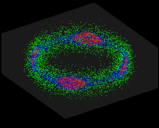
Figure 2: Samples generated at each wave for the torus implausibility function of [50]. At the final level, the adaptive sampler correctly identifies the four regions of the zero-th contour level (in red). It should be noted that exploration of the space could be done with samples from previous levels if required.

4 Sequential non-implausible design

Having successfully identified the NROY space, the question of how to query from such region to refocus the emulator remains a challenging problem. The seminal papers [12] and [13] performed a sequential design for this purpose. The common choice in the literature is to select points greedily from the NROY space to build a new emulator completely focused on that region [40]. This implies that a new emulator is built based on the identified region at every wave. In this work, a different (albeit conservative approach) is followed. Since the simulator is assumed to be computationally very expensive, it might seem unrealistic to expect that the computational budget is kept the same at every wave. Moreover, discarding points might represent a waste of resources and information. In turn, the points must be chosen carefully at each wave to later add them to the set of training runs and build a new GP emulator.

The idea is that the most general information would likely be extracted at the very first iterations while greater accuracy will be pursued at later stages of the history matching procedure. For example, in the first waves a good characterisation of the global trend can potentially be identified. It is therefore appropriate to guide the choice of training points by following suitable learning criteria. This is done in Bayesian optimisation or in reliability analysis problems [6, 32, 48]. For comparison, three active learning criteria are studied.

The first criterion is the expected contour improvement by [38]. The improvement function is defined as

$$\mathcal{I}_{z}(\mathbf{x})=\epsilon^{2}(\mathbf{x})-\min\left\{(f_{\textsf{GP}}(\mathbf{x})-z)^{2},\epsilon^{2}(\mathbf{x})\right\},$$ (4.1)

where $f_{\textsf{GP}}(\mathbf{x})$ is the GP emulator at configuration $\mathbf{x}$, $z$ the targeted contour level, and $\epsilon(\mathbf{x})=k\,v(\mathbf{x})$ the number of predicted standard deviations derived from the uncertainty model, $v(\mathbf{x})=\sqrt{\sigma^{2}(\mathbf{x})+\sigma^{2}_{\text{md}}+\sigma^{2}_{\text{me}}}$. Note that the full uncertainty model is employed in order to be consistent with the preceeding notation. In practice, since both measurement error and model discrepancy are assumed to be constant, this assumption does not affect the history matching pipeline considered here. In the context of simultaneous model calibration and discrepancy learning as in [4, 33] more careful considerations should be taken. For instance, the above points can be addressed by using only the predicted variability of the GP, since the approach developed here aims at improving the emulator. In this setting, $k$ can be chosen as 3, following the three sigma rule. The expected value of the contour improvement is used, given that the emulator is random in nature. The expected contour improvement (ECI) can be computed as

$$\mathbb{E}[\mathcal{I}_{z}(\mathbf{x})]= \left[\epsilon^{2}(\mathbf{x})-(m(\mathbf{x})-z)^{2}-\sigma^{2}(\mathbf{x})\right]\left[\Phi(z_{2})-\Phi(z_{1})\right]$$

$$+\sigma^{2}(\mathbf{x})\,\left[z_{2}\,\phi(z_{2})-z_{1}\,\phi(z_{1})\right]$$ (4.2)

$$+2[m(\mathbf{x})-z]\,\sigma(\mathbf{x})\left[\phi(z_{2})-\phi(z_{1})\right]$$

where $z_{1}=(z-m(\mathbf{x})-\epsilon(\mathbf{x}))/\sigma(\mathbf{x})$, $z_{2}=(z-m(\mathbf{x})+\epsilon(\mathbf{x}))/\sigma(\mathbf{x})$, and $\Phi(\cdot)$ and $\phi(\cdot)$ are the standard Gaussian cumulative and density functions respectively.

The second criterion to be considered is the expected risk by [17], which was originally designed for reliability analysis. This aims at learning the set $\{\mathbf{x}:g(\mathbf{x})>0\}$, with $g(\mathbf{x})$ the performance or limit-state function of a configuration $\mathbf{x}$. The critical level $g(\mathbf{x})=0$ is referred to as a transition level, as its correct emulation classifies a given configuration in terms of the system’s performance. In this paper, the problem is explicitly stated in terms of the contour level $z$ which corresponds to the observed data in the experimental setting. This means that the risk function is defined as

$$R_{z}(\mathbf{x})=\left\{\begin{array}[]{ll}(f_{\textsf{GP}}(\mathbf{x})-z)_{+}&\text{if }m(\mathbf{x})\leq z\\ (z-f_{\textsf{GP}}(\mathbf{x}))_{+}&\text{if }m(\mathbf{x})>z\end{array}\right.,$$ (4.5)

where $(\cdot)_{+}$ denotes the non-negative part of the argument, and $m(\mathbf{x})$ denotes the expected value of the GP emulator at configuration $\mathbf{x}$. The expected risk is used as a learning criterion due to the random nature of the output of the emulator. The derivation is a straightforward solution of one dimensional Gaussian integration, which for completeness is included in Appendix A. The analytical expression can be written in compact form as

$$\mathbb{E}[R_{z}(\mathbf{x})]=\sigma(\mathbf{x})\left[-\text{sign}(\bar{z})\,\bar{z}\,\Phi\left(-\text{sign}(\bar{z}\right)\,\bar{z})+\phi(\bar{z})\right],$$ (4.6)

where $\bar{z}=(z-m(\mathbf{x}))/\sigma(\mathbf{x})$ denotes the standardised contour level, $\text{sign}(\cdot)$ the sign function, and the pair $\Phi(\cdot)$ and $\phi(\cdot)$ are the cumulative and density functions used as before.

The third learning criterion to be compared is a variation of the entropic profile presented by [34]. Originally formulated in the reliability analysis literature, it was designed to measure the entropy of a random variable in a neighbourhood of two standard deviations from the origin. In this paper, the concept has been extended. Again, an explicit solution is presented for a contour level $z$ observed in the experimental data. The entropic profile is defined as

$$H_{z}(\mathbf{x})=\Bigg{|}\int_{z-k\,\sigma(\mathbf{x})}^{z+k\,\sigma(\mathbf{x})}-\ln\pi(f_{\textsf{GP}})\,\pi(f_{\textsf{GP}})\,\mathrm{d}f_{\textsf{GP}}\Bigg{|}.$$ (4.7)

As shown in Appendix B, the entropic profile can be written compactly as

$$H_{z}(\mathbf{x})=\Big{|}\left[\ln\left(\sqrt{2\pi}\,\sigma(\mathbf{x})\right)+0.5\right]\,\left[\Phi(z_{2})-\Phi(z_{1})\right]-0.5\,\left[z_{2}\phi(z_{2})-z_{1}\phi(z_{1})\right]\Big{|},$$ (4.8)

where, as before, $z_{1}$ and $z_{2}$ denote the standardised contour levels.

All the above learning criteria rank the samples from the identified NROY space. It is important to note that this type of criteria take into account a one-step-look-ahead pointwise strategy. Other options include A-optimal designs, which incorporate area impacts to the improvement of the emulator’s response surface. See [10] for a thorough discussion of optimal design of experiments. In particular, following dynamic programming strategies, one can define a learning criteria with a known number of sequential decisions. As a consequence, this type of selection of points choose a batch of candidate runs. This is known as finite-horizon dynamic programming [8], and is subject of future study which falls outside the scope of this paper.

Given the proposed learning criteria, a natural question is how to choose the points in the resulting ranking. Since nearby sample points are likely to be similarly ranked, it would be naive and a waste of computational resources to query the simulator on just the top-ranked NROY samples. Alternatively, to choose uniformly from the sampled points would ignore any ranking at all. An adequate leverage between these extremes is achieved by the following procedure.

Firstly, after a learning criterion has been chosen to rank the samples, a cut off point needs to be selected to specify a subset of good candidates. This cut off is a threshold to guarantee that some percentage of the maximum attainable gain can be held. In this work, this threshold is set to be $50\%$. The rational for this choice is the following. For a very high percentage cut off, the strategy would likely concentrate in narrow neighbourhoods around the highest-ranked sample. In contrast, a very low percentage would not acknowledge the ranking at all. To strike a balance, a conservative approach is to only include those samples able to attain at least a $50\%$ best score. The optimal value for this threshold could be problem-dependent, and a more detailed numerical study is the subject of future research. Once this threshold is set, the first point chosen is the one ranked the highest by the active learning criterion. By construction, the rest of the points above the 50% threshold will have a lower ranking, but will still be desirable samples. In practice, this means that the learning criteria will guide the first points in the rank, whilst the rest should be sampled following a space filling design in order to train the emulator.

Secondly, a maximin design is proposed to choose the next batch of training points from the collection of desirable training runs, that is, points above the cut off value. The seed of this design is selected to be the top ranking point from the NROY samples, i.e. the point that has the highest expected gain. It is important to note that this type of sampling usually starts with the mean of a cloud of points [32]. Since the NROY space has potentially a complicated, possibly disconnected topology, the average point might lie outside the region of interest and choosing a point from outside the NROY space could potentially be a poor selection.

Concretely, the proposed strategy proceeds as follows. After choosing the starting point $\mathbf{x}_{0}$, construct the new set of training points as $\mathcal{D}^{*}=\{\mathbf{x}_{0}\}\cup\mathcal{D}$. The next point selected for the maximin design is the furthest sample available within the NROY space weighted by the cutoff point $\alpha$, denoted by $\mathcal{X}_{\text{NROY}}(\alpha)$, so that

$$\mathbf{x}_{1}=\underset{\mathbf{x}\in\mathcal{X}_{\text{NROY}}(\alpha)\setminus\mathcal{D}^{*}}{\arg\max}\|\mathbf{x}-\mathbf{x}_{0}\|,$$ (4.9)

is chosen as a successor. The new training data is updated accordingly, $\mathcal{D}^{*}\leftarrow\{\mathbf{x}_{1}\}\cup\mathcal{D}^{*}$. The next step computes distances of the sampled points in $\mathcal{X}_{\text{NROY}}(\alpha)$ to the set $\mathcal{D}^{*}$ and retains the candidate farthest apart from $\mathcal{D}^{*}$. This is done iteratively by computing

$$\mathbf{x}_{k}=\underset{\mathbf{x}\in\mathcal{X}_{\text{NROY}}(\alpha)\setminus\mathcal{D}^{*}}{\arg\max}d(\mathbf{x},\mathcal{D}^{*}),$$ (4.10)

where

$$d(\mathbf{x},\mathcal{D}^{*})=\min_{\mathbf{x}^{\prime}\in\mathcal{D}^{*}}\|\mathbf{x}-\mathbf{x}^{\prime}\|,$$ (4.11)

denotes the distance of $\mathbf{x}$ to the current set of training data $\mathcal{D}^{*}$. After every point is found by (4.10), the training dataset is updated accordingly $\mathcal{D}^{*}\leftarrow\{\mathbf{x}_{k}\}\cup\mathcal{D}^{*}$. This procedure is repeated sequentially until $N$ new samples to train a refocused emulator are gathered. As mentioned above, the first point will follow the specific learning criterion chosen. The rest of selected points will followed a space-filling design.

In summary, the use of the maximin selection allwos one to (i) retain the best possible point; (ii) collect samples from a space-filling design in NROY space; and (iii) restrict the choice of new points following the active learning criteria.

5 Numerical experiments

In this section, the performance of the proposed history matching approach is applied to a 2D example, a 3D case study of a fault model, and a battery of multidimensional tests. The 2D example serves as an illustration of the proposed approach. In particular, the maximin design to choose from the ranked samples. The 3D example illustrates a multi-output use of history matching. Finally, the testbed of random functions provides a setting where the approach is tried in different dimensional settings.

In history matching applications, a common stopping rule to terminate the procedure is to compare the maximum predicted error of the emulator in the NROY samples to the estimated variance attributed to measurement and model discrepancy ($\sigma_{\text{me}}^{2}$ and $\sigma_{\text{md}}^{2}$). The motivation is that further improvement of the surrogate would not be able to reduce the elicited deviations from the simulator. The GP, in this setting, is ideal since it provides an estimation of predicted error as a by-product of its construction. As an alternative to this criterion, this work explores the use of a scoring rule, the Continuously Ranked Probability score (CRPS) [25]. It has the properties of being a proper scoring rule to report probabilistic inferences. As stated before, the GP emulator is able to provide full probabilistic statements like predicted values and dispersion estimates around such predictions. The benefit of using the CRPS over local scoring rules like the negative logarithm of predictive density (NLPD) relies on the fact that localised rules risk penalising heavily over-confident predictions whilst treating under-confident and far-off predictions more leniently. In contrast, the CRPS aims for better placement of probability mass near target values, although not exactly placed at the target. The interested reader is refered to [25] and [31] . In particular, it is known that the full Bayesian treatment in GPs is preferred for better error estimation in uncertainty analysis [30] and thus CRPS provides an appropriate scoring rule for GP emulation. This exploits the fact that under the Monte Carlo approximation, the predicted value and variance of the GP emulator is a mixture of Gaussians, as seen in (2.1) and (2.2). The CRPS evaluated at $\mathbf{x}$ corresponds to

$$\text{CRPS}\left(\sum_{k=1}^{N}\omega_{k}\,\mathcal{N}\left(m_{k}(\mathbf{x}),\sigma^{2}_{k}(\mathbf{x})\right)\,,\,z\right)= \sum_{k=1}^{N}\omega_{k}\,A\left(z-m_{k}(\mathbf{x}),\sigma^{2}_{k}(\mathbf{x})\right)$$

$$\quad-\frac{1}{2}\sum_{k=1}^{N}\sum_{l=1}^{N}\omega_{k}\omega_{l}\,A\left(m_{k}(\mathbf{x})-m_{l}(\mathbf{x}),\sigma^{2}_{k}(\mathbf{x})+\sigma^{2}_{l}(\mathbf{x})\right),$$ (5.1)

where $\omega_{k}$ denotes the weight of $k$-th Gaussian component of the mixture, and $m_{k}(\mathbf{x})$ and $\sigma^{2}_{k}(\mathbf{x})$ are the corresponding mean and variance of the GP emulator evaluated at the index $\mathbf{x}$. The function $A(\cdot,\cdot)$ is defined as

$$A(m,\sigma^{2})=2\sigma\phi\left(\frac{m}{\sigma}\right)+m\left(2\,\Phi\left(\frac{m}{\sigma}\right)-1\right),$$ (5.2)

where $\phi(\cdot)$ and $\Phi(\cdot)$ denote the density and cumulative functions of a standard Gaussian random variable. It should be noted that the CRPS is measured in the same units as the output of the simulator and can be evaluated at every location of interest. In this work, we measure the GP predictive capabilities over the NROY space through the samples generated from the strategy described in Section 3. The interested reader is referred to [25] for more properties of the CRPS.

5.1 Franke’s function

This experiment uses Franke’s function as a simulator. It was first introduced in the surrogate modeling literature in [20]. Franke’s function is defined in the two dimensional unit cube, and consists of a sum of three Gaussian peaks and one smaller dip. The function is defined as

$$f(\mathbf{x})=\, \quad\,0.75\,\exp\left(-\frac{(9x_{1}-2)^{2}}{4}-\frac{(9x_{2}-2)^{2}}{4}\right)+0.75\,\exp\left(-\frac{(9x_{1}+1)^{2}}{49}-\frac{9x_{2}+1}{10}\right)$$

$$\,+0.5\,\exp\left(-\frac{(9x_{1}-7)^{2}}{4}-\frac{(9x_{2}-3)^{2}}{4}\right)-0.2\,\exp\left(-(9x_{1}-4)^{2}-(9x_{2}-7)^{2}\right).$$ (5.3)

For the purpose of history matching, the target contour level has been defined as $z=0.6$, which results in two disconnected disks, as shown as a solid red line in Figure 3(a). The dashed red lines correspond to the emulator’s predicted contour level of interest. The shaded regions represent the implausibility contour levels, where lighter colours denote a higher probability. The roughness of the shaded regions is due to the low number of training runs, which translates as a vague posterior distribution for the GP hyperparameters. As previously discussed, when the available training data is small, multimodal samplers are able to represent code uncertainty more robustly [21].

Panels in Figure 3(a) show the sequence of waves of the history matching procedure. The points in blue represent training points that were used to fit the emulator, whereas orange diamonds depict the chosen points by the active learning. For the purpose of illustration, the entropic profile discussed in Section 4 was chosen in Figure 3. The samples generated from the NROY space at each wave are shown in Figure 3(b). In this case, the use of sampling algorithms based on annealed distributions is justified by the complex geometry of the target region [53, 21]. In particular, the first panel in Figure 3(b) shows that all NROY samples satisfy the property of being good candidates to improve the emulator. In the same panel, orange dots denote the chosen points after selecting the top ranking sample shown. For the remaining subpanels in Figure 3(b), light blue dots illustrate sample points from the NROY space which are not suitable to improve the emulator. The best candidates are depicted in dark blue following the ranking from the entropic learning criteria. Also, the space filling interpretation of the maximin strategy is demonstrated empirically in the first panel (the first wave of history matching). As noted before, good coverage can be seen in all panels in Figure 3(b) by the maximin space filling criteria which selects the best candidates to improve the emulator.

    

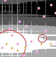
(a) Contour levels and training runs

    

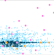
(b) NROY identification and sample selection

Figure 3: Results for Franke’s function in the history matching setting. In Figure 3(a), contour levels of the probability of implausibility are shown with lighter shades. Pink dots represent training runs used for the simulator at wave $t$, and orange diamonds new points identified in NROY space with good predicted improvement performance. Each subpanel in Figure 3(b) shows the samples in NROY space, with those satisfying a good predicted improvement in darker colours. The points selected to run the simulator to improve the GP emulator are shown as orange diamonds.

The procedure was replicated independently 50 times for each learning criteria. This is depicted as boxplots in Figure 4, where results are shown for both the maximum predicted error and the CRPS as iterations advance. For the purpose of visualising the trends, the medians corresponding to each wave are shown connected by a solid line. The predicted errors steadily decrease for each learning criteria. However, it can be seen that the decrements in CRPS are marginal in the last wave. The LHS criterion chooses, among the NROY samples, using the maximin design without any ranking or prescribed threshold. It is important to note that the LHS sampling scheme appears to decrease the predicted error at each wave. This strategy seems to be working well as the emulator is improved in terms of predicting capabilities. However, it should be noted that the other strategies – using learning criteria – are able to improve both the prediction and variability as measured by the CRPS.

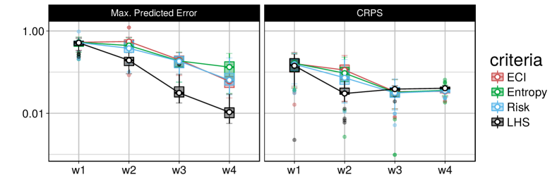
Figure 4: History matching for Franke’s function. The procedure was performed independently 50 times for each of the active learning criteria. The results are summarised in boxplots at each wave. The Maximum predicted error was calculated from the NROY samples at each wave. Analogously, the reported CRPS was computed as the median from the NROY samples. Although a space-filling criterion reduces the predicted error further than the other candidates, the probability statements seem to deteriorate when compared to the other learning criteria.

5.2 The IC fault model

The following experiment tests the proposed history matching framework in a physical model. The IC fault model is a cross-sectional simulator of a reservoir [43]. Each run is determined by three unknown input parameters, namely, $h$ (the fault throw), $k_{g}$ (the good-quality sand permeability) and $k_{h}$ (the poor-quality sand permeability). The complexity of the calibration has made this model become a benchmark to test history matching [40].

The outputs of this simulator are 36-month time series corresponding to three different properties such as oil production rate, water injection rate and water production rate. The information of this model is stored as a collection of 159,661 code runs selected uniformly at random in the 3-dimensional cube. Instead of matching the full time series, only three statistics are chosen as in [40]. Those outputs are $o_{24}$ the oil production rate at month 24; $o_{36}$ the oil production rate at month 36; and $w_{36}$, the water injection rate at month 36.

For experimental purposes, it is assumed that there is no access to such a rich dataset. In turn, a handful of 60 points are chosen at random from a Latin hypercube sampling scheme to initialise the procedure. At each wave, an additional 30 points are selected as discussed in Section 4. This is done to improve the emulator at the pre-specified target level. Each output is emulated independently by a GP. In this case, the implausibility function is a probabilistic version of the Second Maximum Implausibility Measure of [46], computed from the GP posterior distribution using a Monte Carlo estimate. This implausibility is used in order to guard against the possibility that one of the emulators is not performing accurately. The Second Implausibility Measure is defined as

$$I^{(2)}(\mathbf{x})=\max_{i}(\,\{I_{(i)}(\mathbf{x})\}\setminus I^{(1)}(\mathbf{x})\,),$$ (5.4)

where $I_{(i)}$ denotes the implausibility for the $i$-th ouput, and $I^{(1)}$ denotes the largest Implausibility among all outputs. The target level to be matched is defined as

$$\mathbf{z}=(563.6,\,387.5,\,917.2)^{\top}.$$ (5.5)

The full history matching procedure was repeated 50 times, each starting with a different LHS design, and the two performance measures for each wave were recorded. Results are summarised as boxplots in Figure 5. To facilitate the visualisation of the trend, the medians are connected by a solid line in the same way it was done in Figure 4 . It is clear that the expected risk learning criteria is both slower and leads to noisier results for this simulator. In all cases, the oil production rate at month 36, i.e.$o_{36}$, proves too difficult to emulate as seen from the boxplots in Figure 5, which show a slight increase in CRPS and marginal decrease in predicted error. Nonetheless, history matching overcomes this limitation and manages to decrease both the expected predicted error and probabilistic predictions in the target contour level defined in Equation 5.5 for the other outputs. It is important to note that better results can be achieved if a different GP emulator is trained at every contour level as in the spirit of [40]. This work focuses on the properties of using both the complete probabilistic statements from the Bayesian posterior of the computer code and the incorporation of active learning criteria that uses this characterization.

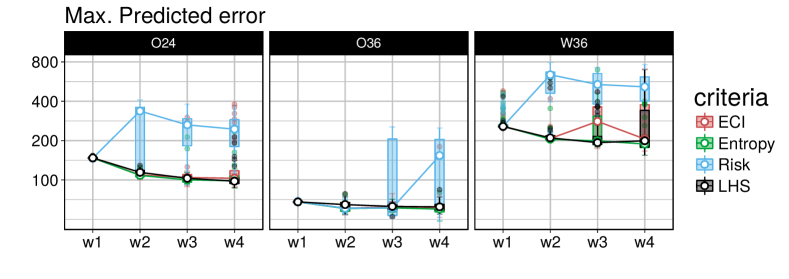
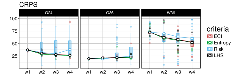
Figure 5: Results for the IC fault model in both performance measurements. Each box corresponds to each output from left to right. By using the probabilistic Second Maximum Implausibility measure it can be noted that there is no bias towards an inaccurate emulator. There is evidence that the oil production rate at month 36, $o_{36}$, proves difficult to fit with the chosen GP assumptions. Nonetheless, the history matching procedure is reducing both the uncertainty and the prediction error for the target contour level.

5.3 Random functions

In order to assess the impact of each learning criteria within the proposed history matching, the following experimental set-up is proposed. It is inspired by [26], as it was used to measure the performance of different acquisition functions used for Bayesian optimisation. The reason to follow this direction is that there is no generally-agreed set of test functions for high dimensions in the history matching literature. The functions to be emulated are generated at random from a GP prior, as shown in Appendix C.

Different dimensionalities are chosen in order to understand both the limitations and strengths of the three active learning criteria for one dimensional output codes. The LHS discussed in the previous experiments is included in the comparison. Having different random seeds, it is possible to replicate the same function for each active learning criteria in each dimensional setting, thus preserving each set of functions to be compared. In total, 50 random functions were simulated in each dimensional setting. For each, the contour level corresponding to the 95% percentile on the prior seeds as explained in Appendix C is chosen as the target for history matching.

The experiments are chosen in order to include low-dimensional spaces (2D and 3D), medium-sized dimensional spaces (5D and 10D) and large dimensional spaces (15D and 20D). In the case of larger dimensional settings, dimensionality reduction techniques can be applied, such as active variable selection [47] or Partial Least Squares [9]. It is widely known that GP tend to lose predictive accuracy and robustness with increasing dimensionality. This happens because the kernel used for the correlation structure relies on some form of Euclidean distance. Thus, the chosen dimensionalities reflect typical feature spaces where the GP emulator is able to generalize well.

In the experiments, history matching is not terminated, but the predicted error is tracked along the iterations. Figure 6 depicts the maximum predicted error at every wave, for each random function. The results are grouped in boxplots to show the overall dispersion at each wave. Once again, the medians are connected with lines between waves for the purpose of better trend visualisation. The space-filling baseline results are shown in black. Overall, the history matching procedure is successful in reducing the maximum predicted error. It is important to note that, in any dimensional setting, the Risk criterion in Equation 4.6 shows less improvement as the waves advance. This is a consequence of the Risk criterion being more susceptible to local exploration than the other candidates. In low-dimensional settings, the Entropic profile and the ECI show a slight advantage over the space-filling design. This is a consequence of a better leverage between the exploitation and exploration trade-off. In high-dimensional settings, both the Entropic profile and the ECI show comparable performance to that of the space-filling design. This is evidence that both criteria are being too general in their rankings and little exploitation of the surrogate is being used.

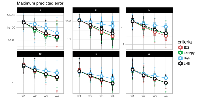
Figure 6: Results for the maximum predicted error in NROY samples. Each subpanel corresponds to different dimensional settings indicated in the black headers. The boxplots are generated by extracting the statistic from each of the replications of the experiment at each wave. Connecting lines are shown to better appreciate the downward trend as the iterations succeed. In all dimensional settings the risk learning criteria is confirmed to be slowest as in Figure 5.

The reduction of the CRPS by the emulation-based history matching is shown in Figure 7, again by the trend in the lines that connect the waves of the procedure. As before, the overall performance is as desired, resulting on decreasing values of the score. The use of the Risk learning criterion seems to be hindered again by its lack of willingness to explore the NROY space as the dimension of the problem increases. As before, the entropic profile and the ECI show comparable results to a space filling design.

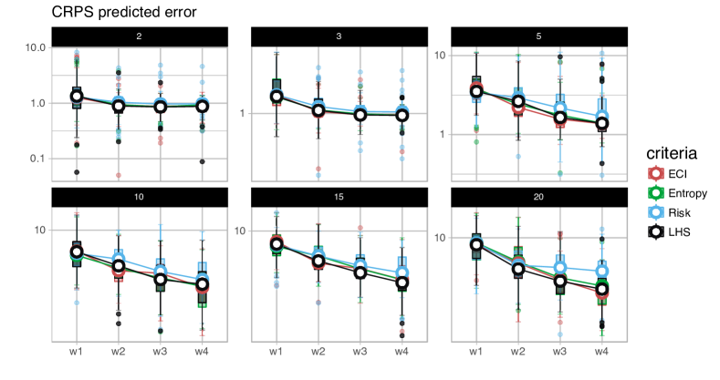
Figure 7: Results for the CRPS predicted error in NROY samples. Each subpanel corresponds to different dimensional settings indicated in the black headers. The boxplots are generated by extracting the statistic from each of the replications of the experiment at each wave. In this case the median of the CRPS is extracted from the NROY samples. Connecting lines are shown to better appreciate the downward trend as the iterations succeed. It should be noted that very low dimensional setting the prediction on the target level do not improves substantially. However, for larger dimensional spaces it continues to improve.

The results show that the Risk learning criterion Equation 4.6 is prone to get trapped in local regions around the best choice. In contrast, for low and medium dimensional settings, the entropic profile and the ECI show a better performance in lowering the maximum predicted error (the variance estimated by the emulator).

For higher dimensional settings, there is no apparent gain in using any of the criteria discussed above. The use of a space-filling design seems like a safe choice. However, it should be noted that the learning criteria do achieve a lower predicted error in low dimensional settings. This should be taken as an indication that something can be done to enhance the performance on higher dimensional problems. Recall that the selection of the samples to refine the emulator is done in two stages. Firstly, the NROY space is identified by an annealed uniform sampling scheme. Secondly, the samples are ranked accordingly (choosing a learning criteria) and those that are not able to produce at least a 50% improvement than the best in the batch are discarded. Following this, amongst the samples retained, a minimax selection procedure is done, starting by the top sample. From the results previously exposed, it seems that setting this 50% target level seems too permissive and that most of the samples are retained in the procedure. In the end, the minimax selection and a space-filling choice become equivalent. This is another embodiment of the curse of dimensionality, in which higher dimensionality requires larger the sampling designs for the emulator. An alternative, which is subject of current research, is to choose a batch of good candidates from the learning criteria as it is done in the Bayesian optimisation setting with the multi-point expected improvement by [11].

6 Conclusions

This paper proposes to acknowledge the probabilistic information of the Gaussian process emulator in history matching applications. This leads to the incorporation of this probabilistic information into the implausibility function. The exploitation of this measure is done by sampling with an annealing schedule as in sequential subset optimisation. This sampling strategy generates uniform samples in the regions defined by a high probability of being non-implausible. In these regions, the simulator is likely to replicate the measured data. The ability to sample from complicated geometries and disconnected regions is achieved by using this form of annealed sampling. These sampling methods have been recently proposed in the Bayesian inference framework but are flexible enough to accommodate to the history matching setting [21]. Additionally, the use of active learning criteria to improve the emulator was also presented. The experimental results show evidence of better performance when using the expected contour improvement or the proposed entropic profile, a version adapted to history matching. This contrasts with random generation of samples by some type of adapted proposals or rejection-based methods. A family of random functions was presented to test the effectiveness of this framework, since there is no agreed collection of history matching test functions. It is important to note that the learning criteria used in this work could arguably be classified as myopic, in the sense that the learning functions only take into account the information available at the current iteration. The extension to finite-horizon criteria, as in Dynamic programming [8], is left as a further research direction. The learning criteria can potentially decrease the number of samples to be considered and achieve comparable results to that of using the whole set of points, as in LHS. Note that theoretical results in [42] show that the GP emulator converges to the true simulator with rates depending on the coverage of the training point design. The experimental results here suggest that certain alternatives can achieve similar consistency. Also, the results shown for the IC-Fault model enhances the need to study further multi-output history matching application. A direction of current research is the use of more general learning criteria, or acquisition functions, that mimic batch optimisation.

References

A Expected risk

The risk criterion is defined by taking into account both the target level $z$ and the predictive probability distribution as learned from the emulator. Note that the output from a GP at index $x$, denoted as $f_{\textsf{GP}}(\mathbf{x})$ is a Gaussian random variable with mean $m(\mathbf{x})$ and variance $\sigma^{2}(\mathbf{x})$. In the following the reference to the index $x$ is omitted to ease the exposition.

The risk criterion is defined as a piecewise function stemming from two possibilities. Firstly, as the shortage of reporting $f_{\textsf{GP}}$ units below the target level $z$ when in expectation it should have reported a greater quantity. Secondly, when the report consisted of $f_{\textsf{GP}}$ units above the target level, when the expected value was known to be below the target. That is, the risk criterion evaluated at index $x$ can be written as

$$R_{z}(\mathbf{x})=\left\{\begin{array}[]{ll}\left(f_{\textsf{GP}}-z\right)_{+}&\text{if }m\leq z\\ \left(z-f_{\textsf{GP}}\right)_{+}&\text{if }m>z\end{array}\right..$$ (A.3)

The expected value of the risk is computed following $f_{\textsf{GP}}\sim\mathsf{N}(m,\sigma^{2})$. The expected risk in the set $m\leq z$ is

$$\mathbb{E}[R_{z}^{-}] =\mathbb{E}[(z-f_{\textsf{GP}})_{+}]$$ (A.4)

$$=\int_{-\infty}^{z}(z-f_{\textsf{GP}})\,\pi(f_{\textsf{GP}})\,\mathrm{d}f_{\textsf{GP}}$$ (A.5)

$$=\sigma\,\left[\left(\frac{z-m}{\sigma}\right)\Phi\left(\frac{z-m}{\sigma}\right)+\phi\left(\frac{z-m}{\sigma}\right)\right]$$ (A.6)

$$=\sigma\,\left[\,\bar{z}\,\Phi(\bar{z})+\phi\left(\bar{z}\right)\right],$$ (A.7)

where $\pi(\cdot)$ denotes the density for the output of the simulator; $(a)_{+}=\max\{0,a\}$; $\bar{z}$, the standardised target level; and, $\Phi$ and $\phi$ the cumulative and density functions of a standard Gaussian random variable. The expected risk can be computed under an analogous procedure for the complementary set as

$$\mathbb{E}[R_{z}^{+}] =\mathbb{E}[(f_{\textsf{GP}}-z)_{+}]$$ (A.8)

$$=\int_{z}^{\infty}(f_{\textsf{GP}}-z)\,\pi(f_{\textsf{GP}})\,\mathrm{d}f_{\textsf{GP}}$$ (A.9)

$$=\sigma\,\left[\,-\bar{z}\,\Phi(-\bar{z})+\phi\left(\bar{z}\right)\right].$$ (A.10)

The expected risk can be computed using the previous results as

$$\mathbb{E}[R_{z}(\mathbf{x})]=\sigma(\mathbf{x})\left[-\text{sign}(\bar{z})\,\bar{z}\,\Phi\left(-\text{sign}(\bar{z}\right)\,\bar{z})+\phi(\bar{z})\right].$$ (A.11)

B Entropic profile

The entropic profile measures the amount of information the emulator $f_{\textsf{GP}}$ contains for the interval comprised of $k$ standard deviations around the target level $z$. Pukelsheim’s rule determines an appropriate $k$ under the assumption of a unimodal distribution for the emulator output to characterise the NROY space. Thus, the entropic profile of the emulator response is computed as

$$H_{z}(\mathbf{x}) =\Biggm{|}-\int_{z-k\sigma}^{z+k\sigma}\log\pi(f_{\textsf{GP}})\,\pi(f_{\textsf{GP}})\,\mathrm{d}f_{\textsf{GP}}\Biggm{|}$$ (B.1)

$$=\Biggm{|}-\int_{z-k\sigma}^{z+k\sigma}\left[-\frac{(f_{\textsf{GP}}-m)^{2}}{2\sigma^{2}}-\log\left(\sqrt{2\pi\sigma^{2}}\right)\right]\,\pi(f_{\textsf{GP}})\,\mathrm{d}f_{\textsf{GP}}\Biggm{|}$$ (B.2)

$$=\Big{|}\left[\ln\left(\sqrt{2\pi\sigma^{2}}\,\right)+0.5\right]\,\left[\Phi(z_{2})-\Phi(z_{1})\right]-0.5\,\left[z_{2}\phi(z_{2})-z_{1}\phi(z_{1})\right]\Big{|},$$ (B.3)

where $z_{1}$ and $z_{2}$ denote the standardised threshold levels of the interval. That is, $z_{1}=(z-m-k\,\sigma)/\sigma$ and $z_{2}=(z-m+k\,\sigma)/\sigma$. The last inequality is obtained after applying well-known properties of the integrals of standard Gaussian densities.

C Random functions from a GP prior

In this paper we propose to generate random test cases from a GP prior as there are no standard test functions for history matching in increasing dimensional settings. This is a similar strategy followed in [26], who used the posterior mean of a GP as a random function.

The process is summarised as follows. For each dimensional setting $d$, we generate $n=100\times d$ points uniformly at random from $[0,1]^{d}$. Let us denote these chosen seeds as ${\bf X}\in\mathbb{R}^{n\times d}$. The lengthscales of a Matèrn kernel, $\boldsymbol{\varphi}$, are generated from a uniform random vector in the cube $[0,2]^{d}$ and the signal noise is chosen as 10. The random choice of seeds and lengthscales generate different functions during this process. The choice of the signal noise to be the same for every test case enables the comparison in terms of predicted error and CRPS among the functions within the same dimensional setting.

The evaluation of the random function is performed as follows. The Gaussian process prior defines a multivariate Gaussian distribution for the output on the seeds $\mathbf{f}\sim\mathsf{N}(0,10^{2}{\bf K})$, where ${\bf K}$ denotes the covariance matrix using the Matérn kernel, the seeds ${\bf X}$ and lengthscales chosen as above. Thus, given a set of training input configurations, say ${\bf X}^{\prime}$, the output of the random function is

$$\mathbf{y}={\bf k}_{*}^{\top}{\bf K}^{-1}\mathbf{f}$$

where ${\bf k}_{*}$ is the column vector of pairwise evaluations of the chosen kernel between each training run ${\bf X}^{\prime}_{i}$ and all random seeds ${\bf X}$.

References

- Andrianakis et al. [2015] I. Andrianakis, I. R. Vernon, N. McCreesh, T. J. McKinley, J. E. Oakley, R. N. Nsubuga, M. Goldstein, and R. G. White. Bayesian History Matching of Complex Infectious Disease Models Using Emulation: A Tutorial and a Case Study on HIV in Uganda. PLoS Computational Biology, 11(1):e1003968, 2015. ISSN 1553-7358. doi: 10.1371/journal.pcbi.1003968. URL http://dx.plos.org/10.1371/journal.pcbi.1003968.
- Andrianakis et al. [2016] I. Andrianakis, I. Vernon, N. McCreesh, T. McKinley, J. Oakley, R. Nsubuga, M. Goldstein, and R. White. History matching of a complex epidemiological model of human immunodeficiency virus transmission by using variance emulation. Journal of the Royal Statistical Society: Series C (Applied Statistics), 2016.
- Andrianakis et al. [2017] I. Andrianakis, N. McCreesh, I. Vernon, T. J. McKinley, J. E. Oakley, R. N. Nsubuga, M. Goldstein, and R. G. White. Efficient history matching of a high dimensional individual-based hiv transmission model. SIAM/ASA Journal on Uncertainty Quantification, 5(1):694–719, 2017.
- Bayarri et al. [2007] M. J. Bayarri, J. O. Berger, R. Paulo, J. Sacks, J. a. Cafeo, J. Cavendish, C.-H. Lin, and J. Tu. A Framework for Validation of Computer Models. Technometrics, 49(2):138–154, 2007. ISSN 0040-1706. doi: 10.1198/004017007000000092.
- Beck and Zuev [2013] J. Beck and K. M. Zuev. Asymptotically Independent Markov Sampling: a new MCMC scheme for Bayesian Inference. International Journal for Uncertainty Quantification, 3(5), 2013.
- Bect et al. [2012] J. Bect, D. Ginsbourger, L. Li, V. Picheny, and E. Vazquez. Sequential design of computer experiments for the estimation of a probability of failure. Statistics and Computing, 22(3):773–793, 2012.
- Berger and Smith [2019] J. O. Berger and L. A. Smith. On the statistical formalism of uncertainty quantification. Annual review of statistics and its application, 6:433–460, 2019.
- Bertsekas [2005] D. P. Bertsekas. Dynamic Programming and Optimal Control, volume 1. Athena Scientific, 2005.
- Bouhlel et al. [2016] M. A. Bouhlel, N. Bartoli, A. Otsmane, and J. Morlier. Improving kriging surrogates of high-dimensional design models by partial least squares dimension reduction. Structural and Multidisciplinary Optimization, 53(5):935–952, 2016.
- Chaloner and Verdinelli [1995] K. Chaloner and I. Verdinelli. Bayesian experimental design: A review. Statistical Science, pages 273–304, 1995.
- Chevalier and Ginsbourger [2013] C. Chevalier and D. Ginsbourger. Fast computation of the multi-points expected improvement with applications in batch selection. In Learning and Intelligent Optimization, pages 59–69. Springer, 2013.
- Craig et al. [1996] P. S. Craig, M. Goldstein, a. H. Seheult, and J. a. Smith. Bayes linear strategies for matching hydrocarbon reservoir history. Bayesian Statistics 5, pages 69–95, 1996. URL http://scholar.google.co.uk/scholar?hl=en&q=Bayes+linear+strategies+for+history+matching+of+hydrocarbon+reservoirs&btnG=&as_sdt=1,5&as_sdtp=#0.
- Craig et al. [1997] P. S. Craig, M. Goldstein, A. H. Seheult, and J. A. Smith. Pressure matching for hydrocarbon reservoirs: a case study in the use of Bayes linear strategies for large computer experiments. In Case studies in Bayesian statistics, pages 37–93. Springer, 1997.
- Cressie [1993] N. A. Cressie. Statistics for Spatial Data. John Wiley & Sons, 1993. ISBN 978-0-471-00255-0.
- DiazDelaO and Adhikari [2011] F. A. DiazDelaO and S. Adhikari. Gaussian process emulators for the stochastic finite element method. International Journal for Numerical Methods in Engineering, 87(6):521–540, 2011.
- Drovandi et al. [2017] C. C. Drovandi, D. J. Nott, and D. E. Pagendam. New insights into history matching via sequential monte carlo. arXiv preprint arXiv:1710.03133, 2017.
- Echard et al. [2013] B. Echard, N. Gayton, M. Lemaire, and N. Relun. A combined importance sampling and kriging reliability method for small failure probabilities with time-demanding numerical models. Reliability Engineering & System Safety, 111:232–240, 2013.
- Eric et al. [2008] B. Eric, N. D. Freitas, and A. Ghosh. Active preference learning with discrete choice data. In Advances in neural information processing systems, pages 409–416, 2008.
- Forrester et al. [2008] A. I. J. Forrester, A. Sóbester, and A. J. Keane. Engineering Design via Surrogate Modelling: A Practical Guide. John Wiley & Sons, 2008. ISBN 9780470060681.
- Franke [1979] R. Franke. A critical comparison of some methods for interpolation of scattered data. Technical report, Monterey, California: Naval Postgraduate School., 1979.
- Garbuno-Inigo et al. [2016] A. Garbuno-Inigo, F. A. DiazDelaO, and K. M. Zuev. Transitional annealed adaptive slice sampling for gaussian process hyper-parameter estimation. International Journal for Uncertainty Quantification, 6(4):341–359, 2016. ISSN 2152-5080.
- Goldstein and Huntley [2016] M. Goldstein and N. Huntley. Bayes linear emulation, history matching, and forecasting for complex computer simulators. Handbook of Uncertainty Quantification, pages 1–24, 2016.
- Goldstein and Wooff [2007] M. Goldstein and D. Wooff. Bayes Linear Statistics, Theory and Methods. Wiley Series in Probability and Statistics. Wiley, 2007. ISBN 9780470065679. URL https://books.google.co.uk/books?id=34Z46xxlIfsC.
- Gong et al. [2016] Z. T. Gong, F. A. DiazDelaO, and M. Beer. Bayesian model calibration using subset simulation. In R. Walls and Bedford, editors, Risk, Reliability and Safety: Innovating Theory and Practice: Proceedings of ESREL 2016, Glasgow, Scotland, September 25-29 2016. CRC Press.
- Grimit et al. [2006] E. P. Grimit, T. Gneiting, V. J. Berrocal, and N. a. Johnson. The continuous ranked probability score for circular variables and its application to mesoscale forecast ensemble verification. Quarterly Journal of the Royal Meteorological Society, 132(621C):2925–2942, 2006. ISSN 00359009. doi: 10.1256/qj.05.235. URL http://doi.wiley.com/10.1256/qj.05.235.
- Hoffman et al. [2011] M. Hoffman, E. Brochu, and N. de Freitas. Portfolio allocation for bayesian optimization. In Proceedings of the Twenty-Seventh Conference on Uncertainty in Artificial Intelligence, pages 327–336. AUAI Press, 2011.
- Holden et al. [2015] P. B. Holden, N. R. Edwards, J. Hensman, and R. D. Wilkinson. Abc for climate: dealing with expensive simulators. arXiv preprint, 2015.
- Jones et al. [1998] D. R. Jones, M. Schonlau, and W. J. Welch. Efficient global optimization of expensive black-box functions. Journal of Global optimization, 13(4):455–492, 1998.
- Kalaitzis and Lawrence [2011] A. A. Kalaitzis and N. D. Lawrence. A simple approach to ranking differentially expressed gene expression time courses through Gaussian process regression. BMC bioinformatics, 12(1):1, 2011. ISSN 1471-2105. doi: 10.1186/1471-2105-12-180. URL http://www.pubmedcentral.nih.gov/articlerender.fcgi?artid=3116489&tool=pmcentrez&rendertype=abstract.
- Kennedy and O’Hagan [2001] M. C. Kennedy and A. O’Hagan. Bayesian calibration of computer models. Journal of the Royal Statistical Society: Series B (Statistical Methodology), 63(3):425–464, Aug. 2001. ISSN 1369-7412. doi: 10.1111/1467-9868.00294. URL http://doi.wiley.com/10.1111/1467-9868.00294.
- Kohonen and Suomela [2006] J. Kohonen and J. Suomela. Lessons learned in the challenge: Making predictions and scoring them. Lecture Notes in Computer Science (including subseries Lecture Notes in Artificial Intelligence and Lecture Notes in Bioinformatics), 3944 LNAI:95–116, 2006. ISSN 16113349. doi: 10.1007/11736790–“˙˝7.
- Kuczera and Mourelatos [2009] R. C. Kuczera and Z. P. Mourelatos. On estimating the reliability of multiple failure region problems using approximate metamodels. Journal of Mechanical Design, 131(12), 2009.
- Liu et al. [2009] F. Liu, M. Bayarri, J. Berger, et al. Modularization in bayesian analysis, with emphasis on analysis of computer models. Bayesian Analysis, 4(1):119–150, 2009.
- Lv et al. [2015] Z. Lv, Z. Lu, and P. Wang. A new learning function for kriging and its applications to solve reliability problems in engineering. Computers & Mathematics with Applications, 70(5):1182–1197, 2015.
- Oakley [2002] J. Oakley. Eliciting Gaussian process priors for complex computer codes. Journal of the Royal Statistical Society Series D: The Statistician, 51(1):81–97, 2002. ISSN 00390526. doi: 10.1111/1467-9884.00300.
- Oakley and O’Hagan [2004] J. E. Oakley and A. O’Hagan. Probabilistic sensitivity analysis of complex models: a Bayesian approach. Journal of the Royal Statistical Society: Series B (Statistical Methodology), 66(3):751–769, Aug. 2004. ISSN 1369-7412. doi: 10.1111/j.1467-9868.2004.05304.x. URL http://doi.wiley.com/10.1111/j.1467-9868.2004.05304.x.
- Pukelsheim [1994] F. Pukelsheim. The three sigma rule. The American Statistician, 48(2):88–91, 1994.
- Ranjan et al. [2008] P. Ranjan, D. Bingham, and G. Michailidis. Sequential experiment design for contour estimation from complex computer codes. Technometrics, 50(4):527–541, 2008.
- Rasmussen and Williams [2006] C. E. Rasmussen and C. K. I. Williams. Gaussian Processes for Machine Learning. MIT Press, 2006. ISBN 026218253X. doi: 10.1142/S0129065704001899.
- Salter and Williamson [2016] J. M. Salter and D. Williamson. A comparison of statistical emulation methodologies for multi-wave calibration of environmental models. Environmetrics, 27(8):507–523, 2016. ISSN 1099-095X. doi: 10.1002/env.2405. URL http://dx.doi.org/10.1002/env.2405. env.2405.
- Smith [2013] R. C. Smith. Uncertainty Quantification: Theory, Implementation, and Applications, volume 12. SIAM, 2013.
- Stuart and Teckentrup [2018] A. Stuart and A. Teckentrup. Posterior consistency for gaussian process approximations of bayesian posterior distributions. Mathematics of Computation, 87(310):721–753, 2018.
- Tavassoli et al. [2005] Z. Tavassoli, J. N. Carter, and P. R. King. An analysis of history matching errors. Computational Geosciences, 9(2):99–123, 2005.
- Tuo and Jeff Wu [2016] R. Tuo and C. Jeff Wu. A theoretical framework for calibration in computer models: parametrization, estimation and convergence properties. SIAM/ASA Journal on Uncertainty Quantification, 4(1):767–795, 2016.
- Vazquez and Bect [2010] E. Vazquez and J. Bect. Convergence properties of the expected improvement algorithm with fixed mean and covariance functions. Journal of Statistical Planning and inference, 140(11):3088–3095, 2010.
- Vernon et al. [2010] I. Vernon, M. Goldstein, and R. G. Bower. Galaxy formation: a Bayesian uncertainty analysis. Bayesian Analysis, 5(4):619–669, Dec. 2010. ISSN 1936-0975. doi: 10.1214/10-BA524. URL http://projecteuclid.org/euclid.ba/1340110846.
- Vernon et al. [2014] I. Vernon, M. Goldstein, R. Bower, et al. Galaxy formation: Bayesian history matching for the observable universe. Statistical Science, 29(1):81–90, 2014.
- Villemonteix et al. [2009] J. Villemonteix, E. Vazquez, and E. Walter. An informational approach to the global optimization of expensive-to-evaluate functions. Journal of Global Optimization, 44(4):509, 2009.
- Wilkinson [2014] R. D. Wilkinson. Accelerating ABC methods using Gaussian processes. AISTATS, pages 1015–1023, 2014.
- Williamson and Vernon [2013] D. Williamson and I. Vernon. Efficient uniform designs for multi-wave computer experiments. arXiv preprint arXiv:1309.3520, 2013.
- Williamson et al. [2013] D. Williamson, M. Goldstein, L. Allison, A. Blaker, P. Challenor, L. Jackson, and K. Yamazaki. History matching for exploring and reducing climate model parameter space using observations and a large perturbed physics ensemble. Climate dynamics, 41(7-8):1703–1729, 2013.
- Yeh et al. [2016] T. Yeh, T. Uvieghara, J. Jennings, C. Chen, F. Alpak, F. Tendo, et al. A practical workflow for probabilistic history matching and forecast uncertainty quantification: Application to a deepwater west africa reservoir. In SPE Annual Technical Conference and Exhibition. Society of Petroleum Engineers, 2016.
- Zuev and Beck [2013] K. M. Zuev and J. L. Beck. Global optimization using the Asymptotically Independent Markov Sampling method. Computers & Structures, 126:107–119, 2013. ISSN 00457949. doi: 10.1016/j.compstruc.2013.04.005. URL http://linkinghub.elsevier.com/retrieve/pii/S0045794913001077.