On the Performance of Non-Orthogonal Multiple Access over Composite Fading Channels

?abstractname?

This paper analyzes the performance of a cooperative relaying non-orthogonal multiple access (NOMA) network over Fisher-Snedecor $\mathcal{F}$ composite fading channels. Specifically, one base station (BS) is assumed to communicate with two receiving mobile users with one acting also as a decode-and-forward (DF) relay. To highlight the achievable performance gains of the NOMA scheme, conventional relaying with orthogonal multiple access (OMA) is also analyzed. For the two systems under consideration, we derive novel exact closed-form expressions for the ergodic capacity along with the corresponding asymptotic representations. The derived expressions are then used to assess the influence of various system parameters, including the fading and shadowing parameters, on the performance of both the NOMA and OMA systems. Monte-Carlo simulation are provided throughout to verify the accuracy of our analysis. Results reveal that the NOMA system can considerably outperform the OMA approach when the power allocation factor is carefully selected. It is also shown that as the fading and/or shadowing parameters are increased, the ergodic capacity performance enhances.

I Introduction

Non-orthogonal multiple access (NOMA) has recently been proposed as a promising solution to overcome many challenges facing the development of the fifth generation (5G) mobile communication networks [1, 2, 3, 4]. In particular, NOMA offers better spectral efficiency, balanced user fairness and reduced access latency, which are crucial for the realization of numerous Internet-of-things (IoT) applications. Unlike orthogonal multiple access (OMA) systems such as frequency-division multiple access (FDMA) and time-division multiple access (TDMA) where orthogonality is maintained in frequency/time domain, NOMA can share the entire time and frequency resources for all served users by superimposing their signals only with different power levels [5, 6, 7, 8].

Numerous studies have recently appeared in the literature analyzing the performance of NOMA-based networks in various wireless communication scenarios. For instance, multiple-input multiple-output (MIMO) techniques were combined with NOMA to provide additional spatial degrees of freedom [9, 10]. NOMA with energy-harvesting (EH) capabilities and various EH protocols were explored in [11, 12, 13, 14, 15]. In addition, physical layer security of NOMA-based networks was considered in a number of recent works [16, 17, 18, 19]. Particularly, however, NOMA in cooperative relaying wireless networks, based on amplify-and-decode (AF) and decode-and-forward (DF) relaying protocols, has recently attracted significant research attention, see e.g., [20, 21, 22, 23, 24, 19, 14, 25, 26] and the references therein. More specifically, the authors in [20] were the first to investigate user cooperation in NOMA systems where users with stronger channel conditions were assigned to assist the other users based on DF relaying. In [21], the authors studied the performance of a cooperative NOMA network with a single dedicated relay helping multiple users using AF and DF schemes. Since more relays provide higher diversity gains, the performance of multi-relay NOMA networks was investigated in [22]. Furthermore, the authors in [23] proposed a joint user and relay selection for cooperative NOMA systems in which multiple users communicate with two destinations through multiple AF relays. In addition, full-duplex relaying in cooperative NOMA systems were studied in [27, 28, 29, 30].

Indeed, all the aforementioned studies have indicated the significance of channel fading characteristics on the communication performance of NOMA-based systems. To the authors’ best knowledge, none of the studies above studied the performance of NOMA networks over composite fading channels which consider concurrently the effects of both multipath fading and shadowing. To fill this gap, this paper is dedicated to analyzing the performance of cooperative relaying NOMA systems in composite fading channels; more specifically, we adopt the recently introduced Fisher-Snedecor $\mathcal{F}$ composite model [31], in which it is assumed that scattered multipath has a Nakagami-$m$ distribution whereas the root-mean-square signal follows an inverse Nakagami-$m$ distribution. The motivation for adopting this channel model is threefold. Firstly, the Fisher-Snedecor $\mathcal{F}$ distribution is accurate and has better tractability compared to other models. Secondly, the $\mathcal{F}$ fading model has been shown to perform better than other composite fading distributions such as generalized-$K$ model in terms of modeling accuracy and computational complexity [32]. Finally, the Fisher-Snedecor $\mathcal{F}$ model includes several fading distributions as special cases, such as Nakagami-$m$ ($m_{s}\rightarrow\infty$) and Rayleigh ($m_{s}\rightarrow\infty,$ $m=1$), where $m_{s}$ and $m$ are the shadowing and fading severity parameters, respectively.

In this work, we consider a NOMA-based cooperative relaying scenario with one base station (BS) communicating directly with two users in the presence of Fisher-Snedecor $\mathcal{F}$ composite fading. The major contributions of this study are summarized as follows.

• We derive novel, closed-form expressions for the probability density function (PDF) and cumulative distribution function (CDF) of the minimum of two Fisher-Snedecor $\mathcal{F}$ random variables (RVs) in terms of the Meijer’s G-function. These fundamental statistics are essential for the computation of the communications performance metrics of interest.

• The exact ergodic capacity expressions of a two-hop DF cooperative system with NOMA and OMA schemes over Fisher-Snedecor $\mathcal{F}$ composite fading channels are derived by utilizing the obtained PDF and CDF expressions.

• The corresponding asymptotic behavior of the ergodic capacity in the high signal-to-noise ratio (SNR) regime is investigated for the two systems under study.

• Through the derived expressions, we examine the impact of various system and fading parameters on the capacity performance. This also allowed us to compare the performance of both the cooperative NOMA and OMA systems. The correctness of the derived analysis is demonstrated by means of equivalent results obtained via Monte-Carlo simulations.

It is worthwhile mentioning that the ergodic capacity expressions are given in terms of special functions such as univariate and multivariate Meijer G-functions, which have recently been extensively used in the literature [33, 34, 35, 36]. Furthermore, although some expressions are expressed in terms of infinite series, they converge rapidly with rather few terms for obtaining a given numerical accuracy.

The rest of this paper is organized as follows. Section II describes the system and channel models considered in this work. In Section III, we characterize the minimum of two Fisher-Snedecor $\mathcal{F}$ RVs and present new closed-form expressions for the corresponding PDF and CDF. In Sections IV and V, we derive closed-form analytical expressions for the ergodic capacity for both the NOMA and conventional cooperative relaying systems over the Fisher-Snedecor $\mathcal{F}$ composite fading channel, respectively. Section VI presents numerical examples of the derived expressions with some insights and discussions of results. Finally, Section VII concludes the paper with a summary of the main results.

The following notations are used in this paper. $f_{X}\left(\cdot\right)$, $F_{X}\left(\cdot\right)$ and $\bar{F}_{X}\left(\cdot\right)$ denote the PDF, CDF and the complementary CDF (CCDF) of the random variable (RV) $X$. $\mathbb{E}\left[\cdot\right]$, $\bigl{|}\cdot\bigr{|}$, $\sum$ and $\prod$ are the expectation, absolute value, summation and product operators. $\textrm{min}\left\{\cdot\right\}$ and $\textrm{ln}\left(\cdot\right)$ represent the minimum argument and the natural logarithm, respectively. The symbol $\left(x\right)_{k}$ is the Pochhammer symbol, $B\left(\cdot,\cdot\right)$ is the Beta function [37, eq. (8.4.2.5)], $\Gamma\left[\cdot\right]$ is the Gamma function [38, eq. 8.310.1], $\psi^{\left(0\right)}\left(\cdot\right)$ is the digamma function, $\textrm{G}_{p,q}^{n,m}\left[\cdot|\cdot\right]$ is the Meijer G-function [38, eq. 9.301], ${}_{2}F_{1}\left(\cdot,\cdot;\cdot;\cdot\right)$ is the Gauss hypergeometric function [37, Eq. (9.100)] and $F_{1}\left(\cdot;\cdot,\cdot;\cdot;\cdot,\cdot\right)$ is the Appell two-variables hypergeometric function [37, Eq. (9.14.1; 9.210)].

II System Model

Let us consider a wireless network illustrated in Fig. 1, which consists of three nodes: a BS, a far user (D) and a near user (R), with the latter acting also as a decode-and-forward (DF) relay operating in half duplex mode. It is assumed that all nodes are equipped with a single antenna and that there exists a direct link between the BS and the far user. The S-to-R, R-to-D and S-to-D channel coefficients are denoted by $h_{\textrm{sr}}$, $h_{\textrm{rd}}$ and $h_{\textrm{sd}}$, respectively, all of which experience independent quasi-static Fisher-Snedecor $\mathcal{F}$ fading. The corresponding instantaneous SNRs of these links are denoted by $\gamma_{i}=\bigl{|}h_{i}\bigr{|}^{2},$ where $i\in\left\{\textrm{sr},\textrm{rd},\textrm{sd}\right\},$ with the PDF in (9).

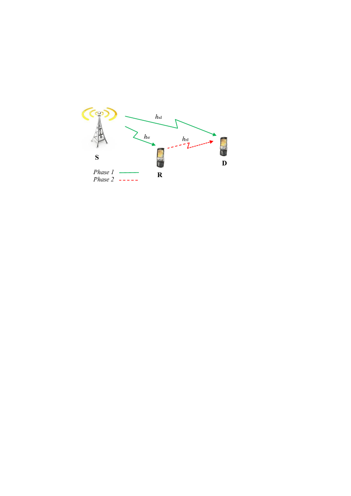
?figurename? 1: The considered NOMA system model with a BS and two users over Fisher-Snedecor $\mathcal{F}$ composite fading channels.

The considered NOMA system requires two time slots to convey information to the two users. In the first time slot, the BS transmits the signal $\sum_{k\in\left\{1,2\right\}}$ $\sqrt{a_{k}P_{s}}s_{k}$ to R and D, where $P_{s}$ is the BS transmit power whereas $a_{1}$ and $a_{2}$ are the power allocation factors for D and R, respectively. Note that $a_{1}+a_{2}=1$ and $a_{1}>a_{2}$. With this in mind, the received signals at R and D can be expressed as

$$y_{i}\left(t\right)=h_{i}\sum_{k\in\left\{1,2\right\}}\sqrt{\frac{a_{k}P_{s}}{d_{i}^{\beta_{i}}}}s_{k}\left(t\right)+n\left(t\right),$$ (1)

where $i\in\left\{\textrm{sr},\textrm{sd}\right\}$ and $n\left(t\right)$ is the noise at R and D which is assumed to be Additive white Gaussian noise (AWGN) with zero mean and variance $\sigma^{2}$, while $\beta_{i}$ and $d_{i}$ are the path-loss exponents and distances from S to R and D. The relay during the first time slot decodes $s_{1}$ and treats $s_{2}$ as noise, and to obtain the latter, the former is canceled using successive interference cancellation (SIC). In this respect, the corresponding SNRs of $s_{1}$ and $s_{2}$ during the first time slot can be written as

$$\gamma_{\textrm{sr}}^{\left(1\right)}=\frac{a_{1}P_{s}\bigl{|}h_{\textrm{sr}}\bigr{|}^{2}}{a_{2}P_{s}\bigl{|}h_{\textrm{sr}}\bigr{|}^{2}+\sigma^{2}},\,\textrm{and}$$ (2)

$$\gamma_{\textrm{sr}}^{\left(2\right)}=\frac{a_{2}P_{s}\bigl{|}h_{\textrm{sr}}\bigr{|}^{2}}{\sigma^{2}}.\hfill$$ (3)

At D, because the symbol $s_{2}$ will be treated as noise during the first time slot, the corresponding SNR is expressed as

$$\gamma_{\textrm{sd}}=\frac{a_{1}P_{s}\bigl{|}h_{\textrm{sd}}\bigr{|}^{2}}{a_{2}P_{s}\bigl{|}h_{\textrm{sd}}\bigr{|}^{2}+\sigma^{2}}.$$ (4)

The relay in the second time slot, assuming that it successfully decoded $s_{2}$, will forward this symbol to D. Therefore, the received signal at D in the second time slot is $y_{\textrm{rd}}\left(t\right)=\sqrt{P_{r}}h_{\textrm{rd}}s_{2}\left(t\right)+n\left(t\right)$ and hence the corresponding SNR is

$$\gamma_{\textrm{rd}}=\frac{P_{r}\bigl{|}h_{\textrm{rd}}\bigr{|}^{2}}{\sigma^{2}},$$ (5)

where $P_{r}$ is the relay transmit power.

III Characterization of the Minimum of Two Fisher-Snedecor $\mathcal{F}$ RVs

In this section, we derived closed-form expressions for the CDF and PDF of the minimum of two Fisher-Snedecor $\mathcal{F}$ variates, which are essential to carry out our analysis in this work. To begin with, let us define two RVs, $\gamma_{x}$ and $\gamma_{y}$, that follow the Fisher-Snedecor $\mathcal{F}$ distribution with PDF [31]

$$f_{\gamma_{i}}\left(\gamma_{i}\right) =\frac{m_{i}^{m_{i}}\left(m_{s_{i}}-1\right)^{m_{s_{i}}}\bar{\gamma}^{m_{s_{i}}}\gamma_{i}^{m_{i}-1}}{B\left(m_{i},\,m_{s_{i}}\right)\left(m\gamma+\left(m_{s_{i}}-1\right)\bar{\gamma}_{i}\right)^{m_{i}+m_{s_{i}}}},$$

$$\stackrel{{\scriptstyle\left(a\right)}}{{=}}\frac{1}{\Gamma\left(m_{i}\right)\Gamma\left(m_{s_{i}}\right)}\gamma_{i}^{-1}\textrm{G}_{1,1}^{1,1}\left[\Lambda_{i}\,\gamma_{i}\Biggl{|}\negthickspace\begin{array}[]{c}1-m_{s_{i}}\\ m_{i}\end{array}\negthickspace\right],m_{s_{i}}>1$$ (8)

while $i\in\left\{x,y\right\}$, $\bar{\gamma}_{i}=\mathbb{E}\left[\gamma_{i}\right]$ is the mean power and $\Lambda_{i}=\frac{m_{i}}{\left(m_{s_{i}}-1\right)\bar{\gamma}_{i}}$, $m_{i}$ and $m_{s_{i}}$ represent respectively the multipath severity and shadowing parameters of the $i$-th RV, respectively. Note that $\left(a\right)$ in (8) is obtained with the aid of [39, Eq. (8.4.2.5)] and [39, Eq. (8.2.2.15)].

Integrating (8) with respect to $\gamma_{i}$, with the help of [40, Eq. (26)], we can express the CDF of $\gamma_{i}$ as

$$F_{\gamma_{i}}\left(\gamma_{i}\right)=\frac{1}{\Gamma\left(m_{i}\right)\Gamma\left(m_{s_{i}}\right)}\,\textrm{G}_{2,2}^{1,2}\left[\Lambda_{i}\gamma_{i}\Biggl{|}\negthickspace\begin{array}[]{c}1-m_{s_{i}},\,1\\ m_{i},\,0\end{array}\negthickspace\right].$$ (9)

Now, let us define the RV

$$\gamma_{z}\triangleq\textrm{min}\left\{\gamma_{x},\,\gamma_{y}\right\},$$ (10)

where $\gamma_{x}$ and $\gamma_{y}$ are independent and non-identically distributed Fisher-Snedecor $\mathcal{F}$ RVs.

With this in mind, the CDF of $\gamma_{z}$ can be obtained as follows

$$F_{\gamma_{z}}\left(u\right)=1-\bar{F}_{\gamma_{x}}\left(u\right)\bar{F}_{\gamma_{y}}\left(u\right),$$ (11)

where $\bar{F}_{\gamma_{i}}\left(u\right)$, is the CCDF of $\gamma_{i}$ which is related to its CDF as $\bar{F}_{\mathcal{X}_{i}}\left(\cdot\right)=1-F_{\mathcal{X}_{i}}\left(\cdot\right)$. Since $\gamma_{x}$ and $\gamma_{y}$ have Fisher-Snedecor $\mathcal{F}$ distribution, their CCDFs can be obtained straightforwardly from (9) with the appropriate notations change. In light of this, using (9) and (11), along performing some straightforward manipulations, the CDF of $\gamma_{z}$ can be expressed as

$$F_{\gamma_{z}}\left(u\right) =\underset{i\in\left\{x,y\right\}}{\sum}\Theta_{i}\,\textrm{G}_{2,2}^{1,2}\left[\,u\,\Biggl{|}\negthickspace\begin{array}[]{c}1-m_{s_{i}},\,1\\ m_{i},\,0\end{array}\negthickspace\right]$$ (14)

$$\qquad-\underset{i\in\left\{x,y\right\}}{\prod}\Theta_{i}\,G_{2,2}^{1,2}\left[\,u\,\Biggl{|}\negthickspace\begin{array}[]{c}1-m_{s_{i}},\,1\\ m_{i},\,0\end{array}\negthickspace\right],$$ (17)

where $\Theta_{i}=1/\left\{\Gamma\left(m_{i}\right)\Gamma\left(m_{s_{i}}\right)\right\}.$

Taking the derivative of $F_{\gamma_{z}}\left(u\right)$, and invoking [39, Eq. (8.2.2.30)], we obtain the PDF of $\gamma_{z}$ as follows

$$\negthickspace\negthickspace\negthickspace f_{\gamma_{z}}\left(z\right)=\underset{i\in\left\{x,y\right\}}{\sum}\Theta_{i}\,G_{3,3}^{1,3}\left[\,z\,\Biggl{|}\negthickspace\begin{array}[]{c}-1,\,-m_{s_{i}},\,0\\ m_{i}-1,\,0,\,-1\end{array}\negthickspace\right]\qquad$$ (20)

$$-\underset{i\in\left\{x,y\right\}}{\prod}\Theta_{i}\,G_{2,2}^{1,2}\left[\,z\,\Biggl{|}\negthickspace\begin{array}[]{c}1-m_{s_{i}},\,1\\ m_{i},\,0\end{array}\negthickspace\right]$$ , (23)

To the authors’ best knowledge, (17) and (23) are new. It is important to mention that, with the help of [39, Eq. (8.2.2.15)], [39, Eq. (8.4.2.5)] and [40, Eq. (17)], the PDF in (23) can also be written in the following form

$$f_{\gamma_{z}}\left(z\right)=\underset{i\in\left\{x,y\right\}}{\sum}\frac{z^{m_{i}-1}\left(1+z\right)^{m_{i}+m_{s_{i}}}}{B\left(m_{i},m_{s_{i}}\right)}-\underset{i\in\left\{x,y\right\}}{\prod}\frac{z^{m_{i}}}{m_{i}}$$

$$\times\frac{1}{B\left(m_{i},m_{s_{i}}\right)}{}_{2}F_{1}\left(m_{i},m_{i}+m_{s_{i}};m_{i}+1;-z\right).$$ (24)

IV Cooperative NOMA over $\mathcal{F}$ Fading Channels

We analyze in this section the exact and asymptotic ergodic sum rate performance of the cooperative NOMA system over the Fisher-Snedecor $\mathcal{F}$ composite fading channels.

IV-A Exact Performance Analysis

The ergodic sum rate of the cooperative NOMA system with DF relaying, $\bar{C}_{\textrm{NOMA}}$, consists of the two rates associated with the symbols $s_{1}$ and $s_{2}$, denoted respectively as $\bar{C}_{1}$ and $\bar{C}_{2}$. That is

$$\bar{C}_{\textrm{NOMA}}=\bar{C}_{1}+\bar{C}_{2}$$ (25)

To simplify our notations and without loss of generality, we assume from now onward that $P=P_{\textrm{s}}=P_{\textrm{r}}$ and $\bar{\gamma}=P/\sigma^{2}$. The achievable rate associated with the first symbol can be calculated as

$$C_{1}=\frac{1}{2}\,\textrm{min}\left\{\textrm{log}_{2}\left(1+\gamma_{\textrm{sr}}^{(1)}\right),\,\textrm{log}_{2}\left(1+\gamma_{\textrm{sd}}\right)\right\},$$ (26)

which, using (2) and (4), can be rewritten as $C_{1}=C_{1,1}-C_{1,2}$, where

$$C_{1,1}=\frac{1}{2}\,\textrm{log}_{2}\left(1+\textrm{min}\left\{\bigl{|}h_{\textrm{sr}}\bigr{|}^{2},\,\bigl{|}h_{\textrm{sd}}\bigr{|}^{2}\right\}\bar{\gamma}\right)\,\textrm{and}$$ (27)

$$C_{1,2} =\frac{1}{2}\,\textrm{log}_{2}\left(1+\textrm{min}\left\{\bigl{|}h_{\textrm{sr}}\bigr{|}^{2},\,\bigl{|}h_{\textrm{sd}}\bigr{|}^{2}\right\}a_{2}\bar{\gamma}\right).$$ (28)

On the other hand, the achievable rate associated with the second symbol can be determined as

$$C_{2} =\frac{1}{2}\,\textrm{min}\left\{\textrm{log}_{2}\left(1+\gamma_{\textrm{sr}}^{(2)}\right),\,\textrm{log}_{2}\left(1+\gamma_{\textrm{rd}}\right)\right\}$$

$$=\frac{1}{2}\,\textrm{log}_{2}\left(1+\textrm{min}\left\{\bigl{|}h_{\textrm{sr}}\bigr{|}^{2}a_{2},\,\bigl{|}h_{\textrm{rd}}\bigr{|}^{2}\right\}\bar{\gamma}\right).$$ (29)

Letting $\mathcal{X}=\textrm{min}\left\{\mathcal{X}_{\textrm{sr}},\,\mathcal{X}_{\textrm{sd}}\right\}$, where $\mathcal{X}_{\textrm{sr}}=\bar{\gamma}\bigl{|}h_{\textrm{sr}}\bigr{|}^{2}$ and $\mathcal{X}_{\textrm{sd}}=\bar{\gamma}\bigl{|}h_{\textrm{sd}}\bigr{|}^{2}$, and using (17) with the appropriate change of variables, we can obtain the CDF of $\mathcal{X}$ as

$$F_{\mathcal{X}}\left(u\right) =\underset{i\in\left\{\textrm{sr},\textrm{sd}\right\}}{\sum}\Theta_{i}\,\textrm{G}_{2,2}^{1,2}\left[\Lambda_{i}\,u\Biggl{|}\negthickspace\begin{array}[]{c}1-m_{s_{i}},\,1\\ m_{i},\,0\end{array}\negthickspace\right]$$ (32)

$$\qquad-\underset{i\in\left\{\textrm{sr},\textrm{sd}\right\}}{\prod}\Theta_{i}\,G_{2,2}^{1,2}\left[\Lambda_{i}\,u\Biggl{|}\negthickspace\begin{array}[]{c}1-m_{s_{i}},\,1\\ m_{i},\,0\end{array}\negthickspace\right],$$ (35)

where $\Theta_{i}=1/\left\{\Gamma\left(m_{i}\right)\Gamma\left(m_{s_{i}}\right)\right\}.$

Taking the derivative of $F_{\mathcal{X}}\left(u\right)$, and with the aid of [39, Eq. (8.2.2.30)], we obtain the PDF of $\mathcal{X}$ as follows

$$\negthickspace\negthickspace\negthickspace f_{\mathcal{X}}\left(z\right)=\underset{i\in\left\{\textrm{sr},\textrm{sd}\right\}}{\sum}\Lambda_{i}\Theta_{i}\,G_{3,3}^{1,3}\left[\Lambda_{i}\,z\Biggl{|}\negthickspace\begin{array}[]{c}-1,\,-m_{s_{i}},\,0\\ m_{i}-1,\,0,\,-1\end{array}\negthickspace\right]\qquad$$ (38)

$$-\underset{i\in\left\{\textrm{sr},\textrm{sd}\right\}}{\prod}\Theta_{i}\,G_{2,2}^{1,2}\left[\Lambda_{i}\,z\Biggl{|}\negthickspace\begin{array}[]{c}1-m_{s_{i}},\,1\\ m_{i},\,0\end{array}\negthickspace\right]$$ . (41)

To this end, the average rate $\bar{C}_{1,1}$ can be obtained as $\bar{C}_{1,1}=\stackrel{{\scriptstyle[}}{{0}}]{\infty}{\int}f_{\mathcal{X}}\left(z\right)$ $\textrm{ln}\left(1+z\right)\textrm{d}z$. Using (41) while expressing the natural logarithmic function in terms of the Meijer G-function, i.e., $\textrm{ln}\left(1+z\right)=G_{2,2}^{1,2}\biggl{[}z|\!\begin{array}[]{c}1,1\\ 1,0\end{array}\!\biggr{]}$, [40, Eq. (11)], we can express $\bar{C}_{1,1}$ as in (53), shown at the top of this page.

$$\bar{C}_{1,1}=\underset{i\in\left\{\textrm{sr},\textrm{sd}\right\}}{\sum}\frac{\Lambda_{i}}{\Gamma\left(m_{i}\right)\Gamma\left(m_{s_{i}}\right)}\underset{I_{1}}{\underbrace{\stackrel{{\scriptstyle[}}{{0}}]{\infty}{\int}G_{3,3}^{1,3}\left[\Lambda_{i}\,z\Biggl{|}\negthickspace\begin{array}[]{c}-1,\,-m_{s_{i}},\,0\\ m_{i}-1,\,0,\,-1\end{array}\negthickspace\right]\textrm{G}_{2,2}^{1,2}\left[z\biggl{|}\!\begin{array}[]{c}1,1\\ 1,0\end{array}\!\right]\textrm{d}z}}-\underset{i\in\left\{\textrm{sr},\textrm{sd}\right\}}{\prod}\frac{1}{\Gamma\left(m_{i}\right)\Gamma\left(m_{s_{i}}\right)}\quad\quad$$ (46)

$$\negthickspace\negthickspace\negthickspace\negthickspace\negthickspace\negthickspace\negthickspace\negthickspace\negthickspace\negthickspace\negthickspace\negthickspace\negthickspace\negthickspace\negthickspace\negthickspace\negthickspace\negthickspace\negthickspace\negthickspace\negthickspace\negthickspace\negthickspace\negthickspace\negthickspace\negthickspace\negthickspace\negthickspace\negthickspace\negthickspace\negthickspace\negthickspace\negthickspace\times\underset{I_{2}}{\underbrace{\stackrel{{\scriptstyle[}}{{0}}]{\infty}{\int}\textrm{G}_{2,2}^{1,2}\left[\Lambda_{\textrm{sr}}\,z\Biggl{|}\negthickspace\begin{array}[]{c}1-m_{s_{\textrm{sr}}},\,1\\ m_{\textrm{sr}},\,0\end{array}\negthickspace\right]G_{2,2}^{1,2}\left[\Lambda_{\textrm{sd}}\,z\Biggl{|}\negthickspace\begin{array}[]{c}1-m_{s_{\textrm{sd}}},\,1\\ m_{\textrm{sd}},\,0\end{array}\negthickspace\right]\textrm{G}_{2,2}^{1,2}\left[z|\!\begin{array}[]{c}1,1\\ 1,0\end{array}\!\right]\textrm{d}z}}.$$ (53)

 

With the help of [37, Eq. (7.811.1)], the integral $I_{1}$ in (53) can be solved as

$$I_{1}=\textrm{G}_{5,5}^{4,3}\left[\frac{1}{\Lambda_{i}}\Biggl{|}\negthickspace\begin{array}[]{c}1-m_{i},\,1,\,1,\,0,\,1\\ 1,\,m_{s_{i}},\,0,\,1,\,0\end{array}\negthickspace\right],$$ (54)

whereas the second integral $I_{2}$ is solved with the aid of [41] as follows

$$I_{2}=\textrm{G}_{2,2:2,2:3,3}^{2,1:1,2:1,3}\left[\Lambda_{i},\Lambda_{l}\Biggl{|}\negthickspace\begin{array}[]{c}-1,0\\ -1,-1\end{array}\negthickspace\Biggl{|}\negthickspace\begin{array}[]{c}1-m_{s_{i}},1\\ m_{i},0\end{array}\negthickspace\Biggl{|}\negthickspace\begin{array}[]{c}-1,-m_{s_{l}},0\\ m_{l}-1,0,-1\end{array}\negthickspace\right],$$ (55)

where $\textrm{ G}_{p_{1},q_{1}:p_{2},q_{2}:p_{3},q_{3}}^{m_{1},n_{1}:m_{2},n_{2}:m_{3},n_{3}}\bigl{[}\cdot\bigr{]}$ is the bivariate Meijer G-function [42].

Substituting (54) and (55) into (53) yields a closed-form expression for average capacity $\bar{C}_{1,1}$ given in (65), shown at the top of the next page.

$$\bar{C}_{1,1}=\underset{i\in\left\{\textrm{sr},\textrm{sd}\right\}}{\sum}\frac{1}{\Gamma\left(m_{i}\right)\Gamma\left(m_{s_{i}}\right)}\,\textrm{G}_{5,5}^{4,3}\left[\frac{1}{\Lambda_{i}}\Biggl{|}\begin{array}[]{c}1-m_{i},\,1,\,1,\,0,\,1\\ 1,\,m_{s_{i}},\,0,\,1,\,0\end{array}\right]$$ (58)

$$-\underset{\underset{i\neq l}{i,l\in\left\{\textrm{sr},\textrm{sd}\right\}}}{\sum}\frac{\Lambda_{l}}{\underset{j\in\left\{\textrm{sr},\textrm{rd}\right\}}{\prod}\Gamma\left(m_{j}\right)\Gamma\left(m_{s_{j}}\right)}\times$$

$$\textrm{ G}_{2,2:2,2:3,3}^{2,1:1,2:1,3}\left[\Lambda_{i},\,\Lambda_{l}\Biggl{|}\begin{array}[]{c}-1,\,0\\ -1,\,-1\end{array}\Biggl{|}\begin{array}[]{c}1-m_{s_{i}},\,1\\ m_{i},\,0\end{array}\Biggl{|}\begin{array}[]{c}-1,-m_{s_{l}},\,0\\ m_{l}-1,\,0,\,-1\end{array}\right]$$ (65)

To find the average capacity $\bar{C}_{1,2}$, let $\mathcal{Y}=\textrm{min}\left\{\mathcal{Y}_{\textrm{sr}},\,\mathcal{Y}_{\textrm{sd}}\right\}$, where $\mathcal{Y}_{\textrm{sr}}=\bar{\gamma}a_{2}\bigl{|}h_{\textrm{sr}}\bigr{|}^{2}$ and $\mathcal{Y}_{\textrm{sd}}=\bar{\gamma}a_{2}\bigl{|}h_{\textrm{sd}}\bigr{|}^{2}$. Following the same procedure used to derive $\bar{C}_{1,1}$, it is straightforward to show that average capacity $\bar{C}_{1,2}$ can be obtained in closed-form as in (75), shown at the top of the next page. The derivation is omitted for the sake of brevity.

$$\bar{C}_{1,2}=\underset{i\in\left\{\textrm{sr},\textrm{sd}\right\}}{\sum}\frac{1}{\Gamma\left(m_{i}\right)\Gamma\left(m_{s_{i}}\right)}\,\textrm{G}_{5,5}^{4,3}\left[\frac{a_{2}}{\Lambda_{i}}\Biggl{|}\negthickspace\begin{array}[]{c}1-m_{i},\,1,\,1,\,0,\,1\\ 1,\,m_{s_{i}},\,0,\,1,\,0\end{array}\negthickspace\right]-\underset{\underset{i\neq k}{i,l\in\left\{\textrm{sr},\textrm{sd}\right\}}}{\sum}\frac{\Lambda_{l}}{\underset{j\in\left\{\textrm{sr},\textrm{rd}\right\}}{\prod}\Gamma\left(m_{j}\right)\Gamma\left(m_{s_{j}}\right)a_{2}}\quad\quad\quad$$ (68)

$$\negthickspace\negthickspace\negthickspace\negthickspace\negthickspace\negthickspace\negthickspace\negthickspace\negthickspace\negthickspace\negthickspace\negthickspace\negthickspace\negthickspace\negthickspace\negthickspace\negthickspace\negthickspace\negthickspace\negthickspace\negthickspace\negthickspace\negthickspace\negthickspace\negthickspace\negthickspace\negthickspace\negthickspace\negthickspace\negthickspace\negthickspace\negthickspace\negthickspace\times\textrm{ G}_{2,2:2,2:3,3}^{2,1:1,2:1,3}\left[\frac{\Lambda_{i}}{a_{2}},\,\frac{\Lambda_{l}}{a_{2}}\Biggl{|}\negthickspace\begin{array}[]{c}-1,\,0\\ -1,\,-1\end{array}\negthickspace\Biggl{|}\negthickspace\begin{array}[]{c}1-m_{s_{i}},\,1\\ m_{i},\,0\end{array}\negthickspace\Biggl{|}\negthickspace\begin{array}[]{c}-1,-m_{s_{l}},\,0\\ m_{l}-1,\,0,\,-1\end{array}\negthickspace\right]$$ (75)

 

Next we derive the average capacity associated with the second symbol $\bar{C}_{2}$. From (29), let $\mathcal{Z}=\textrm{min}\left\{\mathcal{Z}_{\textrm{sr}},\,\mathcal{Z}_{\textrm{sd}}\right\}$, where $\mathcal{Z}_{\textrm{sr}}=\bar{\gamma}a_{2}\bigl{|}h_{\textrm{sr}}\bigr{|}^{2}$ and $\mathcal{Z}_{\textrm{rd}}=\bar{\gamma}\bigl{|}h_{\textrm{rd}}\bigr{|}^{2}$ and following the same steps used to analyze $\mathcal{X}$ and $\mathcal{Y}$, we can express $\bar{C}_{2}$ in closed-form as in (94), shown at the top of the next page.

$$\bar{C}_{2}=\frac{1}{\Gamma\left(m_{\textrm{sr}}\right)\Gamma\left(m_{s_{\textrm{sr}}}\right)}\,\textrm{G}_{5,5}^{4,3}\left[\frac{a_{2}}{\Lambda_{\textrm{sr}}}\Biggl{|}\negthickspace\begin{array}[]{c}1-m_{\textrm{sr}},\,1,\,1,\,0,\,1\\ 1,\,m_{s_{\textrm{sr}}},\,0,\,1,\,0\end{array}\negthickspace\right]+\frac{1}{\Gamma\left(m_{\textrm{rd}}\right)\Gamma\left(m_{s_{\textrm{rd}}}\right)}\,\textrm{G}_{5,5}^{4,3}\left[\frac{1}{\Lambda_{\textrm{rd}}}\Biggl{|}\negthickspace\begin{array}[]{c}1-m_{\textrm{rd}},\,1,\,1,\,0,\,1\\ 1,\,m_{s_{\textrm{rd}}},\,0,\,1,\,0\end{array}\negthickspace\right]\quad\quad\quad$$ (80)

$$\negthickspace\negthickspace\negthickspace\negthickspace\negthickspace\negthickspace\negthickspace\negthickspace\negthickspace\negthickspace\negthickspace\negthickspace\negthickspace\negthickspace\negthickspace\negthickspace\negthickspace\negthickspace\negthickspace\negthickspace\negthickspace\negthickspace\negthickspace\negthickspace\negthickspace\negthickspace\negthickspace\negthickspace\negthickspace\negthickspace\negthickspace\negthickspace\negthickspace-\frac{1}{\underset{j\in\left\{\textrm{sr},\textrm{rd}\right\}}{\prod}\Gamma\left(m_{j}\right)\Gamma\left(m_{s_{j}}\right)}\Biggl{(}\Lambda_{\textrm{rd}}\,\textrm{G}_{2,2:2,2:3,3}^{2,1:1,2:1,3}\left[\Lambda_{\textrm{rd}},\,\frac{\Lambda_{\textrm{sr}}}{a_{2}}\Biggl{|}\negthickspace\begin{array}[]{c}-1,\,0\\ -1,\,-1\end{array}\negthickspace\Biggl{|}\negthickspace\begin{array}[]{c}1-m_{s_{\textrm{sr}}},\,1\\ m_{\textrm{sr}},\,0\end{array}\negthickspace\Biggl{|}\negthickspace\begin{array}[]{c}-1,-m_{s_{\textrm{rd}}},\,0\\ m_{\textrm{rd}}-1,\,0,\,-1\end{array}\negthickspace\right]$$ (87)

$$+\,\frac{\Lambda_{\textrm{sr}}}{a_{2}}\,\textrm{G}_{2,2:2,2:3,3}^{2,1:1,2:1,3}\left[\Lambda_{\textrm{rd}},\,\frac{\Lambda_{\textrm{sr}}}{a_{2}}\Biggl{|}\negthickspace\begin{array}[]{c}-1,\,0\\ -1,\,-1\end{array}\negthickspace\Biggl{|}\negthickspace\begin{array}[]{c}1-m_{s_{\textrm{rd}}},\,1\\ m_{\textrm{rd}},\,0\end{array}\negthickspace\Biggl{|}\negthickspace\begin{array}[]{c}-1,-m_{s_{\textrm{sr}}},\,0\\ m_{\textrm{sr}}-1,\,0,\,-1\end{array}\negthickspace\right]\Biggr{)}$$ (94)

 

IV-B Asymptotic Performance Analysis

In this subsection, we derive asymptotic expressions for the capacity of the cooperative NOMA system. The asymptotic analysis is anchored in obtaining expressions in higher SNR regimes to gain further insight in the system performance. When the SNR $\gamma$ is sufficiently large, such that $\ln\left(1+\gamma\right)\simeq\ln\left(\gamma\right),$ then the asymptotic capacity is given by the following lemma.

Lemma 1.

The asymptotic ergodic capacity of the cooperative NOMA system is expressed as

$$\bar{C}_{\textrm{NOMA}}^{\textrm{asym}}=\bar{C}_{1,1}^{\textrm{asym}}-\bar{C}_{1,2}^{\textrm{asym}}+\bar{C}_{2}^{\textrm{asym}},$$ (95)

where $C_{1,1}^{\textrm{asym}}$ , $C_{1,2}^{\textrm{asym}}$ and $C_{2}^{\textrm{asym}}$ are given by (103), (104) and (105), respectively.

Proof:

At high SNR, the instantaneous capacities in (27), (28) and (29) can be, respectively, reduced to

$$C_{1,1}^{\textrm{asym}}=\frac{1}{2}\,\textrm{log}_{2}\left(\textrm{min}\left\{\bigl{|}h_{\textrm{sr}}\bigr{|}^{2},\,\bigl{|}h_{\textrm{sd}}\bigr{|}^{2}\right\}\bar{\gamma}\right),$$ (96)

$$C_{1,2}^{\textrm{asym}} =\frac{1}{2}\,\textrm{log}_{2}\left(\textrm{min}\left\{\bigl{|}h_{\textrm{sr}}\bigr{|}^{2},\,\bigl{|}h_{\textrm{sd}}\bigr{|}^{2}\right\}a_{2}\bar{\gamma}\right),$$ (97)

$$C_{2}^{\textrm{asym}} =\frac{1}{2}\,\textrm{log}_{2}\left(\textrm{min}\left\{\bigl{|}h_{\textrm{sr}}\bigr{|}^{2}a_{2},\,\bigl{|}h_{\textrm{rd}}\bigr{|}^{2}\right\}\bar{\gamma}\right),$$ (98)

where $\bar{C}_{1,1}^{\textrm{asym}}=\stackrel{{\scriptstyle[}}{{0}}]{\infty}{\int}f_{\mathcal{X}}\left(z\right)$ $\textrm{ln}\left(z\right)\textrm{d}z$, $\bar{C}_{1,2}^{\textrm{asym}}=\stackrel{{\scriptstyle[}}{{0}}]{\infty}{\int}f_{\mathcal{Y}}\left(z\right)$ $\textrm{ln}\left(z\right)\textrm{d}z$ and $\bar{C}_{2}^{\textrm{asym}}$$=\stackrel{{\scriptstyle[}}{{0}}]{\infty}{\int}f_{\mathcal{Z}}\left(z\right)$$\textrm{ln}\left(z\right)\textrm{d}z$.

To compute $\bar{C}_{1,1}^{\textrm{asym}}$, we utilize (24) to rewrite in the form presented in (99), shown at the top of this page

$$\bar{C}_{\textrm{1,1}}^{\textrm{asym}}=\underset{i\in\left\{\textrm{sr},\textrm{sd}\right\}}{\sum}\frac{\Lambda_{i}^{m_{i}}}{B\left(m_{i},m_{s_{i}}\right)}\underset{J_{\textrm{1,1}}}{\underbrace{\stackrel{{\scriptstyle[}}{{0}}]{\infty}{\int}\frac{z^{m_{i}-1}\textrm{ln}\left(z\right)}{\left(1+\Lambda_{i}z\right)^{m_{i}+m_{s_{i}}}}\textrm{d}z}}-\underset{k\in\left\{\textrm{sr},\textrm{sd}\right\}}{\prod}\frac{\Lambda_{k}^{m_{k}}}{B\left(m_{k},m_{s_{k}}\right)}\qquad\hfill\qquad\qquad\qquad\qquad\qquad$$

$$\qquad\hfill\qquad\qquad\qquad\>\times\underset{\underset{i\neq k}{i,l\in\left\{\textrm{sr},\textrm{sd}\right\}}}{\sum}\frac{1}{m_{i}}\underset{J_{\textrm{1,2}}}{\underbrace{\stackrel{{\scriptstyle[}}{{0}}]{\infty}{\int}\frac{z^{m_{i}+m_{l}-1}\textrm{ln}\left(z\right)}{\left(1+\Lambda_{l}z\right)^{m_{l}+m_{s_{l}}}}{}_{1}F_{2}\left(m_{i},m_{i}+m_{s_{i}},m_{i}+1;-\Lambda_{i}z\right)\textrm{d}z}}$$ (99)

 

. The integral $J_{\textrm{1,1}}$ in (99) can be evaluated, with the help of [37, Eq. (4.293.14), (3.458)], as

$$J_{\textrm{1,1}}=\frac{B\left(m_{i},m_{s_{i}}\right)}{\Lambda_{i}^{m_{i}}}\left(\psi^{\left(0\right)}\left(m_{i}\right)-\psi^{\left(0\right)}\left(m_{s_{i}}\right)-\textrm{ln}\left(\Lambda_{i}\right)\right).$$ (100)

Now, to solve the integral $J_{\textrm{1,2}}$ in (99), we first expand the Gauss hypergeometric function in terms of the series representation [37, Eq. (9.14.1)]. Then exchanging the integral and summation order along with some mathematical manipulations, the integral $J_{\textrm{1,2}}$ can be rewritten as

$$J_{\textrm{1,2}}= \stackrel{{\scriptstyle[}}{{n}}=0]{\infty}{\sum}\frac{\left(m_{i}+m_{s_{i}}\right)_{n}\Lambda_{i}^{n}}{\left(m_{i}+1\right)_{n}}$$

$$\times\underset{J_{\textrm{1,3}}}{\underbrace{\stackrel{{\scriptstyle[}}{{0}}]{\infty}{\int}\frac{z^{m_{i}+m_{l}+n-1}\textrm{ln}\left(z\right)}{\left(1+\Lambda_{l}z\right)^{m_{l}+m_{s_{l}}}\left(1+\Lambda_{i}z\right)^{m_{i}+m_{s_{i}}+n}}\textrm{d}z}}.$$ (101)

Note that the transformation in (117) was utilized to arrive at (101). To the authors’ best knowledge, the integral $J_{\textrm{1,3}}$ can not be solved in closed-form in its current form. However, assuming that $m_{s_{i}}-1=Cm_{i}$, where $C\in\mathbb{N}$, we get

$$J_{\textrm{1,3}}= \stackrel{{\scriptstyle[}}{{0}}]{\infty}{\int}\frac{z^{m_{i}+m_{l}+n-1}\textrm{ln}\left(z\right)}{\left(1+\frac{z}{C\bar{\gamma}}\right)^{m_{l}+m_{s_{l}}+m_{i}+m_{s_{i}}+n}}\textrm{d}z,$$

$$\stackrel{{\scriptstyle\left(a\right)}}{{=}} \left(C\bar{\gamma}\right)^{m_{l}+m_{i}+n}B\left(m_{s_{l}}+m_{s_{i}},m_{i}+m_{l}+n\right)$$

$$\left(\psi^{\left(0\right)}\left(m_{i}+m_{l}+n\right)-\psi^{\left(0\right)}\left(m_{s_{i}}+m_{s_{l}}\right)+\textrm{ln}\left(C\bar{\gamma}\right)\right).$$ (102)

Now, substituting (102) into (101), then (101) and (100) into (99), along with some basic algebra, yields

$$\bar{C}_{1,1}^{\textrm{asym}}=\underset{i\in\left\{\textrm{sr},\textrm{sd}\right\}}{\sum}\left(\psi^{\left(0\right)}\left(m_{i}\right)-\psi^{\left(0\right)}\left(m_{s_{i}}\right)-\textrm{ln}\left(\Lambda_{i}\right)\right)\quad\quad$$

$$\negthickspace\negthickspace\negthickspace\negthickspace\negthickspace\negthickspace\negthickspace\negthickspace\negthickspace\negthickspace\negthickspace\negthickspace\negthickspace\negthickspace\negthickspace\negthickspace\negthickspace\negthickspace\negthickspace\negthickspace\negthickspace\negthickspace\negthickspace\negthickspace\negthickspace\negthickspace\negthickspace\negthickspace-\underset{\underset{i\neq l}{i,l\in\left\{\textrm{sr},\textrm{sd}\right\}}}{\sum}\stackrel{{\scriptstyle[}}{{n}}=0]{\infty}{\sum}\frac{B\left(m_{i}+m_{l}+n,m_{s_{i}}+m_{s_{l}}\right)}{B\left(m_{i},m_{s_{l}}\right)B\left(m_{i}+n,m_{s_{i}}\right)\left(m_{l}+n\right)}$$

$$\times\left(\psi^{\left(0\right)}\left(m_{i}+m_{l}+n\right)-\psi^{\left(0\right)}\left(m_{s_{i}}+m_{s_{l}}\right)-\textrm{ln}\left(\bar{\gamma}C\right)\right)$$ (103)

Following the same procedure used to derive (103), it is straightforward to show that $\bar{C}_{1,2}^{\textrm{asym}}$ can be given as in (104), shown at the top of this page.

$$\bar{C}_{1,2}^{\textrm{asym}}=\underset{i\in\left\{\textrm{sr},\textrm{sd}\right\}}{\sum}\left(\psi^{\left(0\right)}\left(m_{i}\right)-\psi^{\left(0\right)}\left(m_{s_{i}}\right)-\textrm{ln}\left(\frac{\Lambda_{i}}{a_{2}}\right)\right)-\underset{\underset{i\neq l}{i,l\in\left\{\textrm{sr},\textrm{sd}\right\}}}{\sum}\stackrel{{\scriptstyle[}}{{n}}=0]{\infty}{\sum}\frac{B\left(m_{i}+m_{l}+n,m_{s_{i}}+m_{s_{l}}\right)}{B\left(m_{i},m_{s_{l}}\right)B\left(m_{i}+n,m_{s_{i}}\right)}$$

$$\qquad\qquad\>\times\frac{1}{\left(m_{l}+n\right)}\left(\psi^{\left(0\right)}\left(m_{i}+m_{l}+n\right)-\psi^{\left(0\right)}\left(m_{s_{i}}+m_{s_{l}}\right)-\textrm{ln}\left(\bar{\gamma}Ca_{2}\right)\right)\hskip 10.00002pt\qquad\hfill$$ (104)

 

. Similarly, we can show that $C_{2}^{\textrm{asym}}$ is given by

$$\bar{C}_{2}^{\textrm{asym}}=\underset{i\in\left\{\textrm{sr},\textrm{sd}\right\}}{\sum}\left(\psi^{\left(0\right)}\left(m_{i}\right)-\psi^{\left(0\right)}\left(m_{s_{i}}\right)-\textrm{ln}\left(\frac{\Lambda_{i}}{a_{2}}\right)\right)\\ -\underset{\underset{i\neq l}{i,l\in\left\{\textrm{sr},\textrm{sd}\right\}}}{\sum}\stackrel{{\scriptstyle[}}{{n}}=0]{\infty}{\sum}\frac{B\left(m_{i}+m_{l}+n,m_{s_{i}}+m_{s_{l}}\right)}{B\left(m_{i},m_{s_{l}}\right)B\left(m_{i}+n,m_{s_{i}}\right)\left(m_{l}+n\right)}\\ \times\left(\psi^{\left(0\right)}\left(m_{i}+m_{l}+n\right)-\psi^{\left(0\right)}\left(m_{s_{i}}+m_{s_{l}}\right)-\textrm{ln}\left(\bar{\gamma}Ca_{2}\right)\right).$$ (105)

This concludes the proof. ∎

V Cooperative OMA over $\mathcal{F}$ Fading Channels

In this section, we analyze the exact and asymptotic ergodic sum rate performance of the cooperative OMA scheme with DF relaying over the Fisher-Snedecor $\mathcal{F}$ composite fading channel.

V-A Exact Performance Analysis

The instantaneous capacity of this system is given by [43, 44, 1]

$$C_{\textrm{OMA}}=\frac{1}{2}\,\textrm{log}_{2}\left(1+\textrm{min}\left\{\bigl{|}h_{\textrm{sr}}\bigr{|}^{2},\,\bigl{|}h_{\textrm{sd}}\bigr{|}^{2}+\bigl{|}h_{\textrm{rd}}\bigr{|}^{2}\right\}\bar{\gamma}\right).$$ (106)

Let $\mathcal{W}=\textrm{min}\left\{\mathcal{W}_{\textrm{sr}},\,\mathcal{W}_{\textrm{sd}}+\mathcal{W}_{\textrm{rd}}\right\}$, where $\mathcal{W}_{i}=\bigl{|}h_{i}\bigr{|}^{2}\bar{\gamma}$ and $i\in\left\{\textrm{sr},\,\textrm{sd},\,\textrm{rd}\right\}$, then the ergodic capacity, $\bar{C}_{\textrm{OMA}}$, can be calculated as

$$\bar{C}_{\textrm{OMA}}=\stackrel{{\scriptstyle[}}{{0}}]{\infty}{\int}\textrm{log}_{2}\left(1+u\right)f_{\mathcal{W}}\left(u\right)\textrm{d}u=\frac{1}{2\textrm{ln}\left(2\right)}\stackrel{{\scriptstyle[}}{{0}}]{\infty}{\int}\frac{F_{\mathcal{W}}\left(u\right)}{1+u}\textrm{d}u,$$ (107)

where $F_{\mathcal{W}}\left(\cdot\right)$ is the CDF of the RV $\mathcal{W}$, which is given by

$$F_{\mathcal{W}}\left(u\right)=1-\bar{F}_{\mathcal{W}_{\textrm{sr}}}\left(u\right)\,\bar{F}_{\mathcal{W}_{\textrm{sd}}+\mathcal{W}_{\textrm{rd}}}\left(u\right),$$ (108)

with $\bar{F}_{\mathcal{W}_{\textrm{sr}}}\left(u\right)$ representing the CCDF of $\mathcal{W}_{\textrm{sr}}$ and $\bar{F}_{\mathcal{W}_{\textrm{sd}}+\mathcal{W}_{\textrm{rd}}}\left(u\right)$ denotes the CCDF of the sum of two Fisher-Snedecor $\mathcal{F}$ variates, $\mathcal{W}_{\textrm{sd}}+\mathcal{W}_{\textrm{rd}}$.

Since the RV $\mathcal{W}_{\textrm{sr}}$ follows the Fisher-Snedecor $\mathcal{F}$ distribution, its CDF $F_{\mathcal{W}_{\textrm{sr}}}\left(\cdot\right)$ can be obtained directly from (9), with the appropriate notation changes, as

$$F_{\mathcal{W}_{\textrm{sr}}}\left(z\right)=\frac{1}{\Gamma\left(m_{\textrm{sr}}\right)\Gamma\left(m_{s_{\textrm{sr}}}\right)}\,G_{2,2}^{1,2}\left[\Lambda_{\textrm{sr}}z\Biggl{|}\negthickspace\begin{array}[]{c}1-m_{s_{\textrm{sr}}},\,1\\ m_{\textrm{sr}},\,0\end{array}\negthickspace\right],$$ (109)

which, after invoking [40, Eq. (17)], can be expressed in terms of the Gauss hypergeometric function as

$$F_{\mathcal{W}_{\textrm{sr}}}\left(z\right)=\Psi z^{m_{\textrm{sr}}}{}_{2}F_{1}\left(m_{\textrm{sr}},m_{\textrm{sr}}+m_{s_{\textrm{sr}}};m_{\textrm{sr}}+1;-\Lambda_{\textrm{sr}}z\right),$$ (110)

where $\Psi=\frac{\Lambda_{\textrm{sr}}^{m_{\textrm{sr}}}}{\textrm{Beta}\left[m_{\textrm{sr}},m_{s_{\textrm{sr}}}\right]m_{\textrm{sr}}}$.

As for the CDF of $\mathcal{W}_{\textrm{sd}}+\mathcal{W}_{\textrm{rd}}$, fortunately, the characterization of the sum of Fisher-Snedecor $\mathcal{F}$ variates has, very recently, been studied in [45]. More specifically, using [45, Eq. (8)], we can express $F_{\mathcal{W}_{\textrm{sd}}+\mathcal{W}_{\textrm{rd}}}\left(\cdot\right)$ as follows

$$F_{\mathcal{W}_{\textrm{sd}}+\mathcal{W}_{\textrm{rd}}}\left(z\right) =\Upsilon z^{2m_{\textrm{rd}}}$$

$$\times {}_{2}F_{1}\left(m_{\textrm{rd}}+m_{s_{\textrm{rd}}},2m_{\textrm{rd}};2m_{\textrm{rd}}+1;-\Lambda_{\textrm{rd}}z\right),$$ (111)

where $\Upsilon=\frac{\Gamma\left[\varpi_{\textrm{rd}}\right]^{2}\Lambda_{\textrm{rd}}^{2m_{\textrm{rd}}}}{\Gamma\left[m_{s_{\textrm{rd}}}\right]^{2}\Gamma\left[2m_{\textrm{rd}}+1\right]}$ and $\varpi_{i}=m_{i}+m_{s_{i}}$. It should be mentioned that (111) is based on the fact that $\mathcal{W}_{\textrm{sd}}$ and $\mathcal{W}_{\textrm{rd}}$ are independent and identically distributed Fisher-Snedecor $\mathcal{F}$ variates.

Now, substituting (110) and (111) into (108) and then into (107), with some algebraic manipulations, we can express $\bar{C}_{\textrm{OMA}}$ as

$$\bar{C}_{\textrm{OMA}} =\frac{1}{2\textrm{ln}\left(2\right)}\left(\mathcal{J}_{1}-\Upsilon\mathcal{J}_{2}-\Psi\mathcal{J}_{3}+\Psi\Upsilon\mathcal{J}_{4}\right),$$ (112)

where $\mathcal{J}_{1},\,\mathcal{J}_{2},\,\mathcal{J}_{3}\,\textrm{and}\,\mathcal{J}_{4}$ are integrals given respectively as

$$\mathcal{J}_{1} =\stackrel{{\scriptstyle[}}{{0}}]{\upsilon}{\int}\frac{1}{1+z}\textrm{d}z=\textrm{ln}\left(1+\upsilon\right),$$ (113)

$$\mathcal{J}_{2} =\stackrel{{\scriptstyle[}}{{0}}]{\upsilon}{\int}\frac{z^{2m_{\textrm{rd}}}}{1+z}{}_{2}F_{1}\left(\varpi_{\textrm{rd}},2m_{\textrm{rd}};2m_{\textrm{rd}}+1;-\Lambda_{\textrm{rd}}z\right)\textrm{d}z,$$ (114)

$$\mathcal{J}_{3} =\stackrel{{\scriptstyle[}}{{0}}]{\upsilon}{\int}\frac{z^{m_{\textrm{sr}}}}{1+z}{}_{2}F_{1}\left(m_{\textrm{sr}},\varpi_{\textrm{sr}};m_{\textrm{sr}}+1;-\Lambda_{\textrm{sr}}z\right)\textrm{d}z,$$ (115)

$$\mathcal{J}_{4}= \stackrel{{\scriptstyle[}}{{0}}]{\upsilon}{\int}\frac{z^{m_{\textrm{sr}}+2m_{\textrm{rd}}}}{1+z}{}_{2}F_{1}\left(\varpi_{\textrm{rd}},2m_{\textrm{rd}};2m_{\textrm{rd}}+1;-\Lambda_{\textrm{rd}}z\right)$$

$$\qquad\times{}_{2}F_{1}\left(m_{\textrm{sr}},\varpi_{\textrm{sr}};m_{\textrm{sr}}+1;-\Lambda_{\textrm{sr}}z\right)\textrm{d}z,$$ (116)

where $\upsilon=1/\Lambda_{\textrm{rd}}$.

We now evaluate the integral $\mathcal{J}_{2}$. It should be noted that the Gauss hypergeometric function in (114) converges only when $\bigl{|}\Lambda_{\textrm{rd}}<1\bigr{|}$. Therefore, in order to overcome this restriction, we use the following transformation [39, Eq. (7.2.4.36)]

$${}_{2}F_{1}\left(a,b;c;x\right) =\left(1-x\right)^{-b}\,_{2}F_{1}\left(c-a;b;c;\frac{x}{x-1}\right).$$ (117)

By using (117) and expanding the Gauss hypergeometric function in terms of the series representation [37, Eq. (9.14.1)], along with some simple mathematical manipulations, we can rewrite $\mathcal{J}_{2}$ as

$$\mathcal{J}_{2} =\stackrel{{\scriptstyle[}}{{n}}=0]{\infty}{\sum}\frac{\left(m_{\textrm{rd}}-m_{s_{\textrm{rd}}}+1\right)_{n}\left(2m_{\textrm{rd}}\right)_{n}}{n!\left(2m_{\textrm{rd}}+1\right)_{n}\Lambda_{\textrm{rd}}^{-n}}\qquad\qquad$$

$$\qquad\hfill\qquad\times\underset{\mathcal{J}_{2,1}}{\underbrace{\stackrel{{\scriptstyle[}}{{0}}]{\upsilon}{\int}\frac{z^{2m_{\textrm{rd}}+n}}{1+z}\left(\frac{1}{\Lambda_{\textrm{rd}}z+1}\right)^{2m_{\textrm{rd}}+n}\textrm{d}z}},$$ (118)

where $\left(x\right)_{k}=\Gamma\left(x+k\right)/\Gamma\left(x\right)$ denotes the Pochhammer symbol defined as

$$\left(b\right)_{n}=\biggl{\{}\begin{array}[]{cc}b\left(b+1\right)\ldots\left(b+n-1\right),&n\in N\\ 1.\hfill\hfill&n\in 0\end{array}$$ (119)

The integral $\mathcal{J}_{2,1}$ in (118) has the form $\int y^{r}$ $\left(1+ay\right)^{p}$$\left(1+by\right)^{q}$ which can be evaluated straightforwardly in closed-form in terms of the Appell hypergeometric function. More specifically, using

$$\stackrel{{\scriptstyle[}}{{0}}]{c}{\int}y^{\alpha} \left(\frac{1}{1+ay}\right)^{\beta_{1}}\left(\frac{1}{1+by}\right)^{\beta_{2}}\textrm{d}z=\frac{c^{\alpha+1}}{\alpha+1}$$

$$\times F_{1}\left(\alpha+1;\beta_{1},\beta_{2};\alpha+2;-ac,-bc\right),$$ (120)

we can evaluate $\mathcal{J}_{2,1}$ as

$$\mathcal{J}_{2,1}= \frac{\Lambda_{\textrm{rd}}^{-\xi}}{\xi}F_{1}\left(\xi;2m_{m_{\textrm{rd}}}+n,1;\psi+1;-1,-\frac{1}{\Lambda_{\textrm{rd}}}\right),$$ (121)

where $\xi=2m_{\textrm{rd}}+n+1.$ Note that the Appell function in (121) converges only when $\bigl{|}\frac{1}{\Lambda_{\textrm{rd}}}<1\bigr{|}$. To overcome this restriction, we use the transformation [39, Eq. (7.2.4.36)]

$$F_{1}\left(a;b_{1},b_{2};c;x_{1},x_{2}\right) =\underset{i\in\left(1,2\right)}{\prod}\left(1-x_{i}\right)^{-b_{i}}$$

$$\times F_{1}\Biggl{(}c-a; b_{1},b_{2};c;\frac{x_{1}}{x_{1}-1},\frac{x_{2}}{x_{2}-1}\Biggr{)}.$$ (122)

Using (122) and (121), along with some algebraic manipulations, we can express $\mathcal{J}_{2}$ in closed-form as follows

$$\mathcal{J}_{2}= \stackrel{{\scriptstyle[}}{{n}}=0]{\infty}{\sum}\frac{\left(m_{\textrm{rd}}-m_{s_{\textrm{rd}}}+1\right)_{n}\left(2m_{\textrm{rd}}\right)_{n}\Lambda_{\textrm{rd}}^{2m_{\textrm{rd}}}}{n!\left(2m_{\textrm{rd}}+1\right)_{n}\left(\Lambda_{\textrm{rd}}+1\right)2^{\left(2m_{\textrm{rd}}+n\right)}\xi}$$

$$\qquad\times F_{1}\left(1;2m_{m_{\textrm{rd}}}+n,1;\xi+1;\frac{1}{2},\frac{1}{\Lambda_{\textrm{rd}}+1}\right).$$ (123)

Following the same procedure used to obtain (123), it is straightforward to evaluate the integral $\mathcal{J}_{3}$. Using the transformation (117) and the series representation of ${}_{2}F_{1}$ [37, Eq. (9.14.1)], we can rewrite $\mathcal{J}_{3}$ as

$$\mathcal{J}_{3} =\stackrel{{\scriptstyle[}}{{l}}=0]{\infty}{\sum}\frac{\left(\varpi_{\textrm{sr}}\right)_{l}\Lambda_{\textrm{sr}}^{l}}{\left(m_{\textrm{sr}}+1\right)_{l}}\underset{\mathcal{J}_{3,1}}{\underbrace{\stackrel{{\scriptstyle[}}{{0}}]{\upsilon}{\int}\frac{z^{-m_{s_{\textrm{sr}}}}}{1+z}\left(\frac{z}{\Lambda_{\textrm{sr}}z+1}\right)^{\varpi_{\textrm{sr}}+l}\textrm{d}z}}.$$ (124)

With the aid of (120), we can evaluate the integral in (124) as

$$\mathcal{J}_{3,1}= \frac{\Lambda_{\textrm{rd}}^{-\phi}}{\phi}\,F_{1}\left(\phi;\varpi_{\textrm{sr}}+l,1;\phi+1;-\frac{\Lambda_{\textrm{sr}}}{\Lambda_{\textrm{rd}}},-\frac{1}{\Lambda_{\textrm{rd}}}\right),$$ (125)

where $\phi=m_{\textrm{sr}}+l+1.$

Substituting (125) into (124), along with some mathematical manipulations, we can express the integral $\mathcal{J}_{3}$ in closed-form as given in (126), shown at the top of the next page. Note that we used $\left(x\right)_{n}=\frac{\Gamma\left(x+n\right)}{\Gamma\left(x\right)}\,\textrm{and}\,\Gamma\left(x+1\right)=x!$ to arrive at (126).

$$\mathcal{J}_{3}=\stackrel{{\scriptstyle[}}{{l}}=0]{\infty}{\sum}\frac{\Gamma\left(\varpi_{\textrm{sr}}+l\right)\Gamma\left(m_{\textrm{sr}}+1\right)\Lambda_{\textrm{sr}}^{l}}{\Gamma\left(\phi+1\right)\Gamma\left(\varpi_{\textrm{sr}}\right)\Lambda_{\textrm{rd}}^{\phi}}\,F_{1}\left(m_{\textrm{sr}}+l+1;\varpi_{\textrm{sr}}+l,1;m_{\textrm{sr}}+l+2;-\frac{\Lambda_{\textrm{sr}}}{\Lambda_{\textrm{rd}}},-\frac{1}{\Lambda_{\textrm{rd}}}\right)$$ (126)

 

Furthermore, to solve the integral $\mathcal{J}_{4}$, we first replace the two Gauss hypergeometric functions in (116) with their series representations, [37, Eq. (9.14.1)], after applying the transformation in (117). This yields (127), shown at the top of the next page. Unfortunately, it is very difficult to evaluate the integral $\mathcal{J}_{\textrm{4,1}}$ in (127) and, to the best of our knowledge, it can not be expressed in closed-form in its current form. However, letting $\left(m_{s_{i}}-1\right)=Cm_{i}$, where $i\in\left\{\textrm{sr},\textrm{rd}\right\}$ and $C\in R$, we can simplify this integral to

$$\mathcal{J}_{4}=\stackrel{{\scriptstyle[}}{{k}}=0]{\infty}{\sum}\stackrel{{\scriptstyle[}}{{m}}=0]{\infty}{\sum}\frac{\left(m_{\textrm{rd}}-m_{s_{\textrm{rd}}}+1\right)_{k}\left(2m_{\textrm{rd}}\right)_{k}}{\left(2m_{\textrm{rd}}+1\right)_{k}\Lambda_{\textrm{rd}}^{-n}k!}\frac{\left(\varpi_{\textrm{sr}}\right)_{m}\Lambda_{\textrm{sr}}^{m}}{\left(m_{\textrm{sr}}+1\right)_{m}} \underset{\mathcal{J}_{\textrm{4,1}}}{\underbrace{\stackrel{{\scriptstyle[}}{{0}}]{\upsilon}{\int}\frac{z^{m_{\textrm{sr}}+2m_{\textrm{rd}}+k+m}}{1+z}\left(\frac{1}{\Lambda_{\textrm{rd}}z+1}\right)^{2m_{\textrm{rd}}+k}\left(\frac{1}{\Lambda_{\textrm{sr}}z+1}\right)^{\varpi_{\textrm{sr}}+m}\textrm{d}z}}$$ (127)

 

$$\mathcal{J}_{\textrm{4,1}}=\frac{\Lambda_{\textrm{rd}}^{-\left(2m_{\textrm{rd}}+n\right)}}{\Lambda_{\textrm{sr}}^{\varpi_{\textrm{sr}}+m}}\stackrel{{\scriptstyle[}}{{0}}]{\upsilon}{\int}\frac{z^{\kappa}}{1+z}\left(\frac{1}{z+C\bar{\gamma}}\right)^{m_{s_{\textrm{sr}}}+\kappa}\textrm{d}z,$$ (128)

where $\kappa=m_{\textrm{sr}}+2m_{\textrm{rd}}+k+m$.

Now, with the aid of (120), $\mathcal{J}_{\textrm{4,1}}$ can be evaluated as

$$\mathcal{J}_{\textrm{4,1}}=\frac{\left(\bar{\gamma}C\right)^{\kappa+1}}{\kappa+1}\,F_{1}\left(\kappa+1;m_{s_{\textrm{sr}}}+\kappa,1;\kappa+2;-1,-\bar{\gamma}C\right).$$ (129)

Now, substituting (129) into (127), along with some rearrangements, yields (130), shown at the top of the next page. Finally, substituting (113), (123), (126) and (130) into (112), we obtain the ergodic capacity of the cooperative OMA system over the Fisher-Snedecor $\mathcal{F}$ composite fading channel.

$$\mathcal{J}_{4}=\stackrel{{\scriptstyle[}}{{k}}=0]{\infty}{\sum}\stackrel{{\scriptstyle[}}{{m}}=0]{\infty}{\sum}\frac{\left(\varpi_{\textrm{sr}}\right)_{m}\left(m_{\textrm{rd}}-m_{s_{\textrm{rd}}}+1\right)_{k}2m_{\textrm{rd}}}{\left(m_{\textrm{sr}}+1\right)_{m}\left(2m_{\textrm{rd}}+n\right)\left(\kappa+1\right)\left(\bar{\gamma}C\right)^{-\left(m_{\textrm{sr}}+2m_{\textrm{rd}}+1\right)}k!} F_{1}\left(\kappa+1;m_{s_{\textrm{sr}}}+\kappa,1;\kappa+2;-1,-\bar{\gamma}C\right)$$ (130)

 

V-B Asymptotic Performance Analysis

In this section, we analysis the asymptotic capacity performance of the cooperative OMA system. At high SNR, the instantaneous capacity in (106) can be simplified to

$$C_{\textrm{OMA}}^{\textrm{asym}}=\frac{1}{2}\,\textrm{log}_{2}\left(\textrm{min}\left\{\bigl{|}h_{\textrm{sr}}\bigr{|}^{2},\,\bigl{|}h_{\textrm{sd}}\bigr{|}^{2}+\bigl{|}h_{\textrm{rd}}\bigr{|}^{2}\right\}\bar{\gamma}\right).$$ (131)

Similar to the analysis in Sec. V, while assuming high SNR regime, it is easy to show that the asymptotic ergodic capacity for the OMA can be given by

$$\bar{C}_{\textrm{OMA}}^{\textrm{asym}} =\frac{1}{2\textrm{ln}\left(2\right)}\left(\mathcal{J}_{1}^{\textrm{asym}}-\Upsilon\mathcal{J}_{2}^{\textrm{asym}}-\Psi\mathcal{J}_{3}^{\textrm{asym}}+\Psi\Upsilon\mathcal{J}_{4}^{\textrm{asym}}\right),$$ (132)

where $\mathcal{J}_{1}^{\textrm{asym}},\mathcal{J}_{2}^{\textrm{asym}},\mathcal{J}_{3}^{\textrm{asym}}\,\textrm{and}\,\mathcal{J}_{4}^{\textrm{asym}}$ are given by $\mathcal{J}_{1}^{\textrm{asym}}=\stackrel{{\scriptstyle[}}{{1}}]{\upsilon}{\int}\frac{1}{z}$$\textrm{d}z$$=\textrm{ln}\left(\upsilon\right)$,

$$\mathcal{J}_{2}^{\textrm{asym}} =\stackrel{{\scriptstyle[}}{{0}}]{\upsilon}{\int}z^{2m_{\textrm{rd}}-1}{}_{2}F_{1}\left(\varpi_{\textrm{rd}},2m_{\textrm{rd}};2m_{\textrm{rd}}+1;-\Lambda_{\textrm{rd}}z\right)\textrm{d}z,$$ (133)

$$\mathcal{J}_{3}^{\textrm{asym}} =\stackrel{{\scriptstyle[}}{{0}}]{\upsilon}{\int}z^{m_{\textrm{sr}}-1}{}_{2}F_{1}\left(m_{\textrm{sr}},\varpi_{\textrm{sr}};m_{\textrm{sr}}+1;-\Lambda_{\textrm{sr}}z\right)\textrm{d}z,$$ (134)

$$\mathcal{J}_{4}^{\textrm{asym}}= \stackrel{{\scriptstyle[}}{{0}}]{\upsilon}{\int}z^{m_{\textrm{sr}}+2m_{\textrm{rd}}-1}{}_{2}F_{1}\left(\varpi_{\textrm{rd}},2m_{\textrm{rd}};2m_{\textrm{rd}}+1;-\Lambda_{\textrm{rd}}z\right)$$

$$\qquad\qquad\times{}_{2}F_{1}\left(m_{\textrm{sr}},\varpi_{\textrm{sr}};m_{\textrm{sr}}+1;-\Lambda_{\textrm{sr}}z\right)\textrm{d}z.$$ (135)

The integral $\mathcal{J}_{2}^{\textrm{asym}}$ in (133), after using the transformation in (117), can be solved as

$$\mathcal{J}_{2}^{\textrm{asym}}= \frac{1}{2m_{\textrm{rd}}\Lambda_{\textrm{rd}}^{2m_{\textrm{rd}}}}\,{}_{3}F_{1}\left(2m_{\textrm{rd}},2m_{\textrm{rd}},\varpi_{\textrm{rd}};A_{\textrm{rd}},A_{\textrm{rd}},-1\right),$$ (136)

where $A_{\textrm{rd}}=2m_{\textrm{rd}}+1$ and ${}_{p}F_{q}\left(\cdot,\cdot,\cdot;\cdot,\cdot,\cdot\right)$ is the generalized hypergeometric function [37, Eq. (9.14.1)]. Similarly, it does not pose any difficulty to show that

$$\mathcal{J}_{3}^{\textrm{asym}}= \frac{1}{m_{\textrm{sr}}\Lambda_{\textrm{rd}}^{m_{\textrm{sr}}}}\,{}_{3}F_{2}\left(m_{\textrm{sr}},m_{\textrm{sr}},\varpi_{\textrm{sr}};A_{\textrm{sr}},A_{\textrm{sr}},-\frac{\Lambda_{\textrm{sr}}}{\Lambda_{\textrm{rd}}}\right),$$ (137)

where $A_{\textrm{sr}}=2m_{\textrm{sr}}+1$.

Now, to solve the integral $\mathcal{J}_{4}^{\textrm{asym}}$, we first apply the transformation in (117) and then replace the two hypergeometric functions with their series representation [37, Eq. (9.14.1)]. Along with some basic algebra and reordering of integration and summations, we can rewrite (135) as

$$\mathcal{J}_{4}^{\textrm{asym}}=\stackrel{{\scriptstyle[}}{{k}}=0]{\infty}{\sum}\stackrel{{\scriptstyle[}}{{m}}=0]{\infty}{\sum}\frac{\left(m_{\textrm{rd}}-m_{s_{\textrm{rd}}}+1\right)_{k}\left(2m_{\textrm{rd}}\right)_{k}}{\left(2m_{\textrm{rd}}+1\right)_{k}\Lambda_{\textrm{rd}}^{-n}k!}\frac{\left(\varpi_{\textrm{sr}}\right)_{m}\Lambda_{\textrm{sr}}^{m}}{\left(m_{\textrm{sr}}+1\right)_{m}}$$

$$\times\underset{\mathcal{J}_{4,1}^{\textrm{asym}}}{\underbrace{\stackrel{{\scriptstyle[}}{{0}}]{\upsilon}{\int}z^{\kappa-1}\left(\frac{1}{\Lambda_{\textrm{rd}}z+1}\right)^{2m_{\textrm{rd}}+k}\left(\frac{1}{\Lambda_{\textrm{sr}}z+1}\right)^{\varpi_{\textrm{sr}}+m}\textrm{d}z}}.$$ (138)

With the help of (120), we can straightforwardly evaluate the integral $\mathcal{J}_{4,1}^{\textrm{asym}}$ in closed-form. At this end, we can now write $\mathcal{J}_{4}^{\textrm{asym}}$ as in (139), given at the top of the next page.

$$\mathcal{J}_{4}^{\textrm{asym}}=\stackrel{{\scriptstyle[}}{{k}}=0]{\infty}{\sum}\stackrel{{\scriptstyle[}}{{m}}=0]{\infty}{\sum}\frac{\left(m_{\textrm{rd}}-m_{s_{\textrm{rd}}}+1\right)_{k}\left(2m_{\textrm{rd}}\right)_{k}\left(\varpi_{\textrm{sr}}\right)_{m}}{\left(2m_{\textrm{rd}}+1\right)_{k}\left(m_{\textrm{sr}}+1\right)_{m}k!}\frac{\Lambda_{\textrm{sr}}^{m}}{\kappa\Lambda_{\textrm{rd}}^{\kappa-k}} \,F_{1}\left(\kappa;\varpi_{\textrm{sr}}+m,2m_{\textrm{rd}}+k;\kappa+1;-\frac{\Lambda_{\textrm{sr}}}{\Lambda_{\textrm{rd}}},-1\right)$$ (139)

 

Finally, substituting $\mathcal{J}_{1}^{\textrm{asym}}$, $\mathcal{J}_{2}^{\textrm{asym}}$, $\mathcal{J}_{3}^{\textrm{asym}}$ and $\mathcal{J}_{4}^{\textrm{asym}}$ into (132) yields a closed-form expression for the asymptotic ergodic capacity of the cooperative OMA system over Fisher-Snedecor $\mathcal{F}$ composite fading channels.

VI Results and Discussions

In this section, we present some numerical examples of the analytical expressions derived above along with Monte-Carlo simulations. All evaluations herein, unless specified otherwise, are based on the following system parameters: $m_{\textrm{sr}}=m_{\textrm{rd}}=m_{\textrm{sd}}=5$, and $C=3$.

To begin with, we plot in Fig. 2 the analytical and simulated ergodic capacity with respect to the average SNR for both the cooperative NOMA and OMA systems over the $\mathcal{F}$ fading channel with different multipath and shadowing conditions when the power allocation factor $a_{2}=0.01$. It is clear from this figure that the analytical and simulated results are in good agreement, which verifies the accuracy of our analysis. Note that the analytical results for the NOMA and OMA systems are obtained from (25) and (107), respectively. It is evident that the NOMA approach outperforms the conventional one when SNR is relatively high, as shown in the extract in Fig. 2b, whereas the OMA approach tends to have better performance at low SNR values (Fig. 2a). Another observation worth highlighting is that as the fading parameter $m_{i}$ is increased, the performance of both systems are enhanced. This is justified by the fact that increasing $m_{i}$ implies increasing the number of multipath clusters arriving at the receiving node which consequently improves the received SNR. This positively influences the ergodic capacity performance. To further emphasize the versatility of the derived expressions, we present the effect of the fading parameters under special cases of one-sided Gaussian ($m_{i}$ = 0.5), Rayleigh ($m_{i}$ = 1) and Nakagami-$m$ ($m_{i}$ = 2) channels in Fig. 2b. As can be observed, the ergodic capacity improvement is clearly evident as the fading severity $m_{i}$ is changed. Furthermore, Fig. 2a also presents the asymptotic ergodic capacity curves of the cooperative NOMA and OMA systems; these results are obtained using (LABEL:eq:NOMAasym) and (132). It is visible that in the high SNR regime, the asymptotic curves are in very good agreement with the exact results and this indeed verify the accuracy of the derived asymptotic capacity expressions.

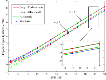
(a) Exact and asymptotic capacity for NOMA and OMA schemes. Fading parameter $m_{i}=\{1,5\}$

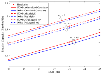
(b) Close-up extract of ergodic capacity for NOMA and OMA at high SNR. One-sided Gaussian ($m_{i}$ = 0.5), Rayleigh ($m_{i}$ = 1), Nakagami-$m$ ($m_{i}$ = 2).

?figurename? 2: Ergodic capacity as a function of $\bar{\gamma}$ for both the cooperative NOMA and OMA schemes over the Fisher-Snedecor $\mathcal{F}$ composite fading channel, when $a_{2}=0.01$ and varying fading parameter $m_{i}$, where $i\in\left\{\textrm{sr},\textrm{rd},\textrm{sd}\right\}.$

To illustrate the impact of the power allocation factor on the system performance, we present in Fig. 3 the ergodic capacity versus the power allocation factor $a_{2}$ with different values of $\bar{\gamma}$ and fading parameters. The performance of the cooperative OMA system is also included in this plot for the sake of comparison. It is interesting to see that when $a_{2}$ is either too small or too large, the performance of the NOMA approach degrades considerably which results in relatively poor performance compared to the OMA scheme. It is also noted that the performance gap between the two systems becomes more pronounced when $\textrm{SNR}=25\textrm{dB}$ compared to the case when $\textrm{SNR}=20\textrm{dB}$. Similarly, in Fig. 4, we plot the ergodic capacity versus the power allocation factor $a_{1}$ with different values of $\bar{\gamma}$ and fading parameters. Again, it can be observed that the performance of the NOMA scheme varies considerably when $a_{1}$ is either too small or too large. This performance mirrors the change in $a_{2}$ as expected since $a_{1}+a_{2}=1.$ Furthermore, in Figs. 3 and 4, the presence of a maxima indicates that when the power allocation factor is carefully selected, the NOMA approach is able to offer better performance, which means that optimizing this factor is crucial to maximizing the performance of the NOMA system.

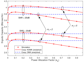
?figurename? 3: Ergodic capacity with respect to the power allocation factor of $R,$ $a_{2}$ and various $\bar{\gamma}$ values. The fading parameter $m_{i}=\{2,5\}$, where $i\in\left\{\textrm{sr},\textrm{rd},\textrm{sd}\right\}.$ Results for the cooperative OMA scheme are also shown.

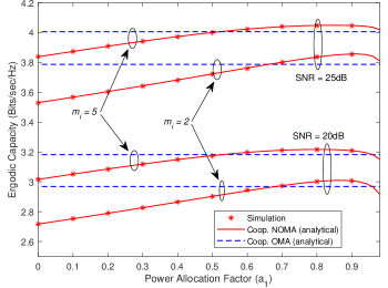
?figurename? 4: Ergodic capacity with respect to the power allocation factor of $D,$ $a_{1}$ and various $\bar{\gamma}$ values. The fading parameter $m_{i}=\{2,5\}$, where $i\in\left\{\textrm{sr},\textrm{rd},\textrm{sd}\right\}.$ Results for the cooperative OMA scheme are also shown.

In Fig. 5, we present the ergodic capacity of both NOMA and OMA schemes as a function of the shadowing parameters of the various links. Here we assume the fading parameters $m_{\textrm{sr}}=m_{\textrm{rd}}=m_{\textrm{sd}}=2$ and $C=2$. Also, while plotting the curves for the shadowing parameters on one link, we assume a fixed shadowing parameter for the other 2 links (moderate shadowing $m_{s_{i}}=4$). We first observe that for regions with severe shadowing $m_{s}<2$, the NOMA S-to-D link provides the best ergodic capacity, while the NOMA R-to-D link rapidly becomes improved to a similar capacity. Further decrease in the shadowing severity (as $m_{s}\longrightarrow\infty)$ presents noticeable improvements. On the other hand, for the OMA scheme, the capacities of both the S-to-D and R-to-D links are fairly even (and lower) through all the regions. The best capacity improvements for the system can however be achieved when the shadowing severity becomes moderate to low i.e. $m_{s}>2$, because for the S-to-R link, both the NOMA and OMA schemes perform much better. This performance increase can be attributed to the configuration of the system with power allocation factor of 90% in favor of this link. Therefore, this further indicates the importance of selecting an appropriate power allocation factor.

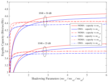
?figurename? 5: Ergodic capacity of NOMA and OMA schemes as a function of the shadowing parameters of S-to-R ($m_{s_{\textrm{sr}}}$), R-to-D ($m_{s_{\textrm{rd}}}$) and S-to-D ($m_{s_{\textrm{sd}}}$) links for various $\bar{\gamma}$ values.

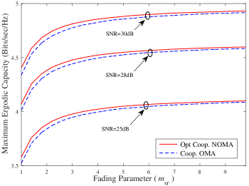
?figurename? 6: Maximum achievable ergodic capacity of the NOMA system over the Fisher-Snedecor $\mathcal{F}$ composite fading channel versus $m_{\textrm{sr}}$ for different values of $\bar{\gamma}$. Note that it is assumed here that $m_{\textrm{rd}}=m_{\textrm{sd}}=5.$

Next, we investigate the impact of optimizing the power allocation parameter $a_{2}$ on the ergodic capacity performance. It should be mentioned that due to the complexity of the derived expression in (25), it is not possible to obtain the optimal $a_{2}$ in closed-form. However, it does not pose any difficulty to obtain numerical solutions using software tools. In this respect, extensive simulations were conducted to find the maximum achievable ergodic capacity that corresponds to the optimal $a_{2}$. Fig. 6 depicts the maximum achievable ergodic capacity versus the fading parameter $m_{\textrm{sr}}$ for $\bar{\gamma}=25\textrm{dB},\,28\textrm{dB}\,\textrm{and}\,30\textrm{dB}$, when $m_{\textrm{rd}}=m_{\textrm{sd}}=5$. One can clearly see from these results that the optimized NOMA system always outperforms the conventional one for all the system configurations under study. It is also worthwhile pointing out that increasing the fading parameter of the S-to-R link will improve the capacity for both cooperative NOMA and OMA systems.

VII Conclusion

This paper has been devoted to the analysis of cooperative relaying wireless networks based on NOMA over Fisher-Snedecor $\mathcal{F}$ composite fading channels. The performance of conventional cooperative relaying systems, i.e., based on OMA, has also been studied for the sake of completeness and comparison. For both the NOMA and OMA systems under consideration, we have derived exact and asymptotic closed-form expressions of the ergodic capacity in terms of special functions and converging power series. These expressions have been used to investigate the impact of various system and fading parameters on the capacity performance. Results have shown that the NOMA approach is able to achieve better performance compared to the OMA scheme in the high SNR region. Results have also demonstrated the positive impact of the multipath fading and the shadowing parameters on the system performance. In addition, optimizing the power allocation factor in the NOMA system is crucial to maximizing the average capacity.

• [1] J. B. Kim and I. H. Lee, “Capacity analysis of cooperative relaying systems using non-orthogonal multiple access,” IEEE Commun. Lett., vol. 19, pp. 1949–1952, Nov. 2015.
• [2] Z. Ding, Z. Yang, P. Fan, and H. V. Poor, “On the performance of non-orthogonal multiple access in 5G systems with randomly deployed users,” IEEE Signal Process. Lett., vol. 21, pp. 1501–1505, Dec. 2014.
• [3] Y. Saito, A. Benjebbour, Y. Kishiyama, and T. Nakamura, “System-level performance evaluation of downlink non-orthogonal multiple access (noma),” in Proc. IEEE Annual Int. Symp. Personal, Indoor, and Mobile Radio Commun. (PIMRC), pp. 611–615, Sept. 2013.
• [4] X. Li, J. Li, Y. Liu, Z. Ding, and A. Nallanathan, “Residual Transceiver Hardware Impairments on Cooperative NOMA Networks,” IEEE Trans. Wireless Commun., vol. 19, no. 1, pp. 680–695, 2020.
• [5] Z. Ding, Y. Liu, J. Choi, Q. Sun, M. Elkashlan, C. L. I, and H. V. Poor, “Application of non-orthogonal multiple access in LTE and 5G networks,” IEEE Commun. Mag., vol. 55, pp. 185–191, Feb. 2017.
• [6] Z. Yang, Z. Ding, P. Fan, and N. Al-Dhahir, “The impact of power allocation on cooperative non-orthogonal multiple access networks with SWIPT,” IEEE Trans. Wireless Commun., vol. 16, pp. 4332–4343, Jul. 2017.
• [7] Q. Yang, H. M. Wang, D. W. K. Ng, and M. H. Lee, “NOMA in downlink SDMA with limited feedback: Performance analysis and optimization,” IEEE J. Sel. Areas Commun., vol. 35, pp. 2281–2294, Oct. 2017.
• [8] K. M. Rabie, B. Adebisi, E. H. G. Yousif, H. Gacanin, and A. M. Tonello, “A comparison between orthogonal and non-orthogonal multiple access in cooperative relaying power line communication systems,” IEEE Access, vol. 5, pp. 10118–10129, 2017.
• [9] J. Choi, “Minimum Power Multicast Beamforming With Superposition Coding for Multiresolution Broadcast and Application to NOMA Systems,” IEEE Trans. Commun., vol. 63, pp. 791–800, Mar. 2015.
• [10] Z. Ding, F. Adachi, and H. V. Poor, “The Application of MIMO to Non-Orthogonal Multiple Access,” IEEE Trans. Wireless Commun., vol. 15, pp. 537–552, Jan. 2016.
• [11] S. K. Zaidi, S. F. Hasan, and X. Gui, “Evaluating the Ergodic Rate in SWIPT-Aided Hybrid NOMA,” IEEE Commun. Lett., vol. 22, pp. 1870–1873, Sep. 2018.
• [12] M. Moltafet, P. Azmi, N. Mokari, M. R. Javan, and A. Mokdad, “Optimal and fair energy efficient resource allocation for energy harvesting-enabled-pd-noma-based hetnets,” IEEE Trans. Wireless Commun., vol. 17, pp. 2054–2067, Mar. 2018.
• [13] L. Pei, Z. Yang, C. Pan, W. Huang, M. Chen, M. Elkashlan, and A. Nallanathan, “Energy-efficient D2D communications underlaying NOMA-based networks with energy harvesting,” IEEE Commun. Lett., vol. 22, pp. 914–917, May 2018.
• [14] X. Li, M. Liu, C. Deng, D. Zhang, X. Gao, K. M. Rabie, and R. Kharel, “Joint Effects of Residual Hardware Impairments and Channel Estimation Errors on SWIPT Assisted Cooperative NOMA Networks,” IEEE Access, vol. 7, pp. 135499–135513, 2019.
• [15] X. Li, J. Li, and L. Li, “Performance Analysis of Impaired SWIPT NOMA Relaying Networks Over Imperfect Weibull Channels,” IEEE Syst. J., vol. 14, no. 1, pp. 669–672, 2020.
• [16] B. Zheng, M. Wen, C. X. Wang, X. Wang, F. Chen, J. Tang, and F. Ji, “Secure NOMA Based Two-Way Relay Networks Using Artificial Noise and Full Duplex,” IEEE J. Sel. Areas Commun., vol. 36, pp. 1426–1440, Jul. 2018.
• [17] B. He, A. Liu, N. Yang, and V. K. N. Lau, “On the Design of Secure Non-Orthogonal Multiple Access Systems,” IEEE J. Sel. Areas Commun., vol. 35, pp. 2196–2206, Oct. 2017.
• [18] Y. Liu, Z. Qin, M. Elkashlan, Y. Gao, and L. Hanzo, “Enhancing the physical layer security of non-orthogonal multiple access in large-scale networks,” IEEE Trans. Wireless Commun., vol. 16, pp. 1656–1672, Mar. 2017.
• [19] X. Li, M. Zhao, X. Gao, L. Li, D. Do, K. M. Rabie, and R. Kharel, “Physical Layer Security of Cooperative NOMA for IoT Networks Under I/Q Imbalance,” IEEE Access, vol. 8, pp. 51189–51199, 2020.
• [20] Z. Ding, M. Peng, and H. V. Poor, “Cooperative non-orthogonal multiple access in 5G systems,” IEEE Commun. Lett., vol. 19, pp. 1462–1465, Aug. 2015.
• [21] J. B. Kim and I. H. Lee, “Non-Orthogonal Multiple Access in Coordinated Direct and Relay Transmission,” IEEE Commun. Lett., vol. 19, pp. 2037–2040, Nov. 2015.
• [22] Z. Ding, H. Dai, and H. V. Poor, “Relay Selection for Cooperative NOMA,” IEEE Wireless Commun. Lett., vol. 5, pp. 416–419, Aug. 2016.
• [23] D. Deng, L. Fan, X. Lei, W. Tan, and D. Xie, “Joint user and relay selection for cooperative NOMA networks,” IEEE Access, vol. 5, pp. 20220–20227, 2017.
• [24] Z. Yang, Z. Ding, Y. Wu, and P. Fan, “Novel Relay Selection Strategies for Cooperative NOMA,” IEEE Trans. Veh. Technol., vol. 66, pp. 10114–10123, Nov. 2017.
• [25] X. Tian, Q. Li, X. Li, H. Peng, C. Zhang, K. M. Rabie, and R. Kharel, “I/Q imbalance and imperfect SIC on two-way relay NOMA systems,” Electronics, vol. 9, no. 2, p. 249, 2020.
• [26] X. Li, Q. Wang, H. Peng, H. Zhang, D. Do, K. M. Rabie, R. Kharel, and C. C. Cavalcante, “A Unified Framework for HS-UAV NOMA Networks: Performance Analysis and Location Optimization,” IEEE Access, vol. 8, pp. 13329–13340, 2020.
• [27] X. Yue, Y. Liu, S. Kang, A. Nallanathan, and Z. Ding, “Spatially Random Relay Selection for Full/Half-Duplex Cooperative NOMA Networks,” IEEE Trans. Commun., vol. 66, pp. 3294–3308, Aug. 2018.
• [28] L. Zhang, M. Xiao, J. Liu, G. Wu, D. Lin, and S. Li, “Outage probability analysis and optimization in downlink NOMA systems with cooperative full-duplex relaying,” in IEEE Veh. Technol. Conf. (VTC-Fall), pp. 1–5, Sep. 2017.
• [29] L. Zhang, J. Liu, M. Xiao, G. Wu, Y. C. Liang, and S. Li, “Performance Analysis and Optimization in Downlink NOMA Systems With Cooperative Full-Duplex Relaying,” IEEE J. Sel. Areas Commun., vol. 35, pp. 2398–2412, Oct. 2017.
• [30] X. Li, M. Liu, C. Deng, P. T. Mathiopoulos, Z. Ding, and Y. Liu, “Full-Duplex Cooperative NOMA Relaying Systems With I/Q Imbalance and Imperfect SIC,” IEEE Wireless Commun. Lett., vol. 9, no. 1, pp. 17–20, 2020.
• [31] S. K. Yoo, S. L. Cotton, P. C. Sofotasios, M. Matthaiou, M. Valkama, and G. K. Karagiannidis, “The Fisher-Snedecor $\mathcal{F}$ distribution: A simple and accurate composite fading model,” IEEE Commun. Lett., vol. 21, pp. 1661–1664, Jul. 2017.
• [32] O. S. Badarneh, P. C. Sofotasios, S. Muhaidat, S. L. Cotton, K. Rabie, and N. Al-Dhahir, “On the secrecy capacity of Fisher-Snedecor $\mathcal{F}$ fading channels,” in 14th Int. Conf. Wireless Mobile Comput., Netw. Commun. (WiMob), pp. 102–107, Oct. 2018.
• [33] E. Balti and M. Guizani, “Mixed RF/FSO Cooperative Relaying Systems with Co-Channel Interference,” IEEE Trans. Commun., vol. 66, no. 9, pp. 4014–4027, 2018.
• [34] H. Lei, H. Luo, K. H. Park, Z. Ren, G. Pan, and M. S. Alouini, “Secrecy outage analysis of mixed RF-FSO systems with channel imperfection,” IEEE Photon. J., vol. 10, pp. 1–13, Jun. 2018.
• [35] G. Nauryzbayev, K. M. Rabie, M. Abdallah, and B. Adebisi, “On the performance analysis of WPT-based dual-hop AF relaying networks in $\alpha$-$\mu$ fading,” IEEE Access, vol. 6, pp. 37138–37149, 2018.
• [36] K. An, M. Lin, W. P. Zhu, Y. Huang, and G. Zheng, “Outage performance of cognitive hybrid satellite-terrestrial networks with interference constraint,” IEEE Trans. Veh. Technol., vol. 65, pp. 9397–9404, Nov. 2016.
• [37] I. S. Gradshteyn and I. M. Ryzhik, Table of Integrals, Series, and Products. 7th ed. Academic Press, Califonia, 2007.
• [38] I. S. Gradshteyn and I. M. Ryzhik, Table of Integrals, Series and Products. 6th ed. New York: Academic, 2000.
• [39] A. P. Prudnikov, Y. A. Brychkov, and O. I. Marichev, Integrals, and Series: More Special Functions. Gordon and Breach Sci. Publ., New York, 1990, vol. 3.
• [40] V. S. Adamchik and O. I. Marichev, “The algorithm for calculating integrals of hypergeometric type functions and its realization in reduce systems,” in Proc. Intern. Conf. on Symbolic and Algebraic Computation, pp. 212–224, 1990.
• [41] “Wolfram research, meijeg. [online]..” available at: http://functions. wolfram.com/HypergeometricFunctions/MeijerG/21/02/04/0001/.
• [42] T. H. Nguyen and S. B. Yakubovich, The Double Mellin-Barnes Type Integrals and Their Applications to Convolution Theory. 1st ed. World Scientific, 1992.
• [43] T. Cover and A. E. Gamal, “Capacity theorems for the relay channel,” IEEE Trans. Inf. Theory, vol. 25, pp. 572–584, Sept. 1979.
• [44] K. Woradit, T. Q. S. Quek, W. Suwansantisuk, H. Wymeersch, L. Wuttisittikulkij, and M. Z. Win, “Outage behavior of selective relaying schemes,” IEEE Trans. Wireless Commun., vol. 8, pp. 3890–3895, Aug. 2009.
• [45] O. S. Badarneh, D. B. da Costa, P. C. Sofotasios, S. Muhaidat, and S. L. Cotton, “On the Sum of Fisher–Snedecor $\mathcal{F}$ Variates and Its Application to Maximal-Ratio Combining,” IEEE Wireless Commun. Lett., vol. 7, pp. 966–969, Dec. 2018.