Sparse Bayesian mass-mapping with uncertainties:
full sky observations on the celestial sphere

Abstract

To date weak gravitational lensing surveys have typically been restricted to small fields of view, such that the flat-sky approximation has been sufficiently satisfied. However, with Stage iv@ surveys (e.g. LSST and Euclid) imminent, extending mass-mapping techniques to the sphere is a fundamental necessity. As such, we extend the sparse hierarchical Bayesian mass-mapping formalism presented in previous work to the spherical sky. For the first time, this allows us to construct maximum a posteriori spherical weak lensing dark-matter mass-maps, with principled Bayesian uncertainties, without imposing or assuming Gaussianty. We solve the spherical mass-mapping inverse problem in the analysis setting adopting a sparsity promoting Laplace-type wavelet prior, though this theoretical framework supports all log-concave posteriors. Our spherical mass-mapping formalism facilitates principled statistical interpretation of reconstructions. We apply our framework to convergence reconstruction on high resolution N-body simulations with pseudo-Euclid masking, polluted with a variety of realistic noise levels, and show a significant increase in reconstruction fidelity compared to standard approaches. Furthermore we perform the largest joint reconstruction to date of the majority of publicly available shear observational datasets (combining DESY1, KiDS450 and CFHTLens) and find that our formalism recovers a convergence map with significantly enhanced small-scale detail. Within our Bayesian framework we validate, in a statistically rigorous manner, the community’s intuition regarding the need to smooth spherical Kaiser-Squires estimates to provide physically meaningful convergence maps. Such approaches cannot reveal the small-scale physical structures that we recover within our framework.

1 Introduction

Gravitational lensing is an astrophysical phenomenon through which the geometry of distant galaxies becomes distorted by the intervening matter distribution. Mathematically, this lensing effect is a perturbation by the local matter topology of the null geodesics along which photons travel (Grimm & Yoo, 2018; Bartelmann & Schneider, 2001; Schneider, 2005). As such, gravitational lensing is sensitive to all matter (both visible and invisible) and is thus a natural tool with which to probe the nature of dark matter.

Weak gravitational lensing refers to the vast majority of lensing events for which images are not multiply sourced or ‘strongly lensed’. Equivalently the weak lensing regime can be defined as the regime in which the lensing perturbations remain (to a good approximation) linear. At first order the effect of weak lensing on distant galaxy images manifests itself as two quantities: the spin-0 magnification referred to as the convergence field ${}_{0}\kappa$, and a spin-2 perturbation to the ellipticity (third-flattening) referred to as the shearing or shear field ${}_{2}\gamma$.

Due to the ‘mass-sheet degeneracy’ there is no way to construct a priori estimates of the intrinsic brightness, hence the convergence field is an unobservable quantity – theoretically one could infer the convergence field directly from the galaxy sizes, but the intrinsic dispersion is too high (Alsing et al., 2015). However, as the distribution of instrinsic ellipticities has zero mean and sufficiently tight dispersion, averaging sufficient observations within a given pixel can provide an accurate estimator for the shear signal. As such, measurements of the shear field ${}_{2}\gamma$ are typically taken and inverted to form estimates of ${}_{0}\kappa$ –  coined dark matter mass maps by Clowe et al. (2006).

A large proportion (Taylor et al., 2018) of cosmological information can be extracted directly from the shear field (Van Waerbeke et al., 2013; Fluri et al., 2019; Giblin et al., 2018), however recently cosmologists have become increasingly interested in extracting information from higher order statistics, such as peak & void statistics and Minkowski functionals, which are typically calculated directly from the convergence field (e.g. Munshi & Coles, 2017; Coles & Chiang, 2000; Peel et al., 2018; Fluri et al., 2018) –  motivating research into optimal mass-mapping techniques. Typically, these higher order statistics aim to probe the non-Gaussian information content of the convergence field.

Mapping from shear to convergence (mass-mapping) requires solving an (often seriously) ill-posed inverse problem –  mass-mapping takes the form of a typical noisy deconvolution problem with a spin-2 kernel (Wallis et al., 2017a), which is classically ill-posed. The most naive mass-mapping technique for small fields of view is planar Kaiser-Squires (KS; Kaiser & Squires, 1993) which is direct inversion of the forward model in Fourier space. This estimator does not take into account noise or boundary effects, and so is typically post-processed via convolution with a large Gaussian smoothing kernel, thus heavily degrading the quality of high-resolution non-Gaussian information. Moreover, decomposition of spin-fields on bounded manifolds is known to be degenerate (Bunn et al., 2003) and so for non-trivial masking the KS estimator is ill-defined and can be shown to perform poorly (see Section 5).

Many, perhaps more sophisticated, approaches to mass-mapping on the plane have been developed (e.g. VanderPlas et al., 2011; Lanusse et al., 2016; Jeffrey et al., 2018; Jee et al., 2016) though all either lack a principled statistical framework or rely heavily on assumptions or impositions of Gaussianity. In previous work we present a sparse hierarchical Bayesian formalism for planar mass-mapping (Price et al., 2018, 2019b; Price et al., 2019a) that provides fully principled statistical uncertainties without the need to assume Gaussianity and without the computational overhead of MCMC methods (e.g. Schneider et al., 2015; Corless et al., 2009; Alsing et al., 2016).

One key assumption of these ‘planar’ mass-mapping techniques is that the area of interest on the sky can be well approximated as a plane. This assumption is colloquially referred to as the the flat-sky approximation. For small-field surveys this approximation is typically justified. However for future wide-field Stage iv@ surveys mass-mapping must be constructed natively on the sphere (Chang et al., 2018) to avoid errors due to projection effects, which can be large (Wallis et al., 2017a; Vallis et al., 2018). Naturally one can naively invert the spherical forward model to form the spherical Kaiser-Squires estimator (SKS; Wallis et al., 2017a) which avoids projection effects but is seriously ill-posed, as is the KS method. It should be noted that alternative techniques for spherical reconstruction have also been developed (e.g. Pichon et al., 2010).

In this paper we extend the previously developed hierarchical Bayesian-sparse formalism to the sphere which, for the first time, allows maximum a posteriori (MAP) convergence reconstruction with principled Bayesian uncertainties in very high-dimensions natively on the sphere without making any assumptions or impositions of Gaussianity. Throughout this paper we refer to our estimator, formed within this framework, as the DarkMapper estimator (and by extension the DarkMapper codebase). The reconstruction formalism presented in this paper and any uncerainty quantification techniques that follow support any choice of likelihood or prior such that the posterior function belongs to the (rather comprehensive) set of log-concave functions. As such one can incorporate various experimental or systematic effects in future, e.g. more complex noise models or intrinsic alignment corrections etc.

The structure of this paper is as follows. In Section 2 we provide background mathematical details relevant to the scope of this paper, such as the analysis of spin signals on the sphere, and succiently review weak gravitational lensing. Following this Section 3 provides a cursory introduction to Bayesian analysis before presenting and discussing both the general hierarchical Bayesian formalism and our DarkMapper estimator. In this section we explicitly outline the likelihood and priors used throughout this paper but place emphasis on the generality of this formalism. Furthermore, we outline how to fold uncertainty in regularization parameters into the hierarchy via the allocation of a suitable (here a conjugate) hyper-prior distribution. In Section 4 we extend previously developed uncertaintiy quantification techniques to the spherical space and discuss how one should approach constructing custom uncertainty quantification techniques which fit within our formalism. In sections 5, using high resolution N-body (Takahashi et al., 2017) simulations, pseudo-Euclid masking (a masking of the galactic plane and the ecliptic) and noise realisations representative of a variety of weak lensing survey eras ( including Stage iv@) we demonstrate the drastic increase in reconstruction fidelity of DarkMapper over SKS. Penultimately, in Section 6 we apply both the SKS and DarkMapper estimators to a global weak lensing dataset constructed via the concatenation of the majority of publicly available observational datasets. To the best of our knowledge this is the first such global spherical dark-matter mass-maps. Furthermore, we perform global Bayesian uncertainty quantification on these reconstructions. Finally, in Section 7 we draw conclusions.

2 Background

Here we present a cursory synopsis of the relevant background required to understand weak lensing on the sphere. In no way is this a complete description and so we recommend the reader follow related papers (Wallis et al., 2017b; Wallis et al., 2017a; McEwen et al., 2015b).

2.1 Spin-s Spherical Fields

Local rotations by $\chi\in[0,2\pi)$ about the tangent plane centered on the spherical coordinate $\omega=(\theta,\psi)\in\mathbb{S}^{2}$ of square integrable spin-s fields for $s\in\mathbb{Z}$ are defined generally by (Goldberg et al., 1967; Newman & Penrose, 1966; Wallis et al., 2017a; McEwen et al., 2013a)

$${}_{s}f^{\prime}(\omega)=e^{-is\chi}{}_{s}f(\omega),$$ (1)

where $\omega=(\theta,\psi)$ are standard spherical coordinates, given by co-latitude $\theta\in[0,\pi)$ and longitude $\psi\in[0,2\pi)$. The natural set of orthogonal basis functions for spherical fields are the spherical harmonics $Y_{\ell m}(\omega)$.

When considering spin-s fields on $\mathbb{S}^{2}$ the natural set of orthogonal basis functions are the spin-weighted spherical harmonics. The spin weighted spherical harmonics are generated by application of the spin raising and lowering operators ($\eth$ and $\bar{\eth}$ respectively) to the spherical eigenfunctions $Y_{\ell m}(\omega)$. The spin-s raising and lowering operators are given respectively, by

$$\eth\equiv-\sin^{s}\theta\Big{(}\frac{\partial}{\partial\theta}+\frac{i\partial}{\sin\theta\partial\psi}\Big{)}\sin^{-s}\theta,$$ (2)

$$\bar{\eth}\equiv-\sin^{-s}\theta\Big{(}\frac{\partial}{\partial\theta}-\frac{i\partial}{\sin\theta\partial\psi}\Big{)}\sin^{s}\theta.$$ (3)

On application to ${}_{s}Y_{\ell m}(\omega)$ we find the recursion relations,

$$\eth\;{}_{s}Y_{\ell m}(\omega) =\big{[}(\ell-s)(\ell+s+1)\big{]}^{1/2}\;{}_{s+1}Y_{\ell m}(\omega),$$ (4)

$$\bar{\eth}\;{}_{s}Y_{\ell m}(\omega) =-\big{[}(\ell+s)(\ell-s+1)\big{]}^{1/2}\;{}_{s-1}Y_{\ell m}(\omega).$$ (5)

Following these recursions it is clear that any spin-s weighted spherical harmonic can be represented as $s\in\mathbb{N}$ repeated applications of the spin raising (lowering) operator $\eth$ to the standard spin-0 spherical harmonic $Y_{\ell m}$ such that,

$${}_{s}Y_{\ell m}(\omega)=\Big{[}\frac{(\ell-s)!}{(\ell+s)!}\Big{]}^{\frac{1}{2}}\;\eth^{s}Y_{\ell m}(\omega),$$ (6)

for positive semi-definite spin $0\leq s\leq\ell$, and for negative semi-definite spin $-\ell\leq s\leq 0$ by,

$${}_{s}Y_{\ell m}(\omega)=(-1)^{s}\Big{[}\frac{(\ell+s)!}{(\ell-s)!}\Big{]}^{\frac{1}{2}}\;\bar{\eth}^{-s}Y_{\ell m}(\omega).$$ (7)

The spin-s weighted spherical harmonics form a complete set of orthogonal basis functions which leads to the harmonic representation of a spin-s field ${}_{s}f(\omega)$ by

$${}_{s}f(\omega)=\sum^{\infty}_{\ell=0}\sum^{\ell}_{m=-\ell}{}_{s}\hat{f}_{\ell m}\;{}_{s}Y_{\ell m}(\omega).$$ (8)

We can then trivially invert this decomposition to give the spin-s field ${}_{s}f(\omega)$ projected onto the spin basis eigenfunctions (i.e. the spin-spherical harmonic coefficients),

$${}_{s}\hat{f}_{\ell m}=\int_{\mathbb{S}^{2}}d\Omega(\omega)\;{}_{s}f(\omega)\;{}_{s}Y_{\ell m}^{*}(\omega),$$ (9)

where the integral is over the sphere $\mathbb{S}^{2}$, and $d\Omega(\omega)=\sin\theta d\theta d\phi$ is the rotation invariant measure on the sphere. Typically the signal is band-limited at $\ell_{\text{max}}$ which implies ${}_{s}f_{\ell m}=0,\forall\ell\geq\ell_{\text{max}}$ allowing the $\ell$ summations in equation (8) and the upper limit of the integral in equation (9) to be truncated at $\ell_{\text{max}}$ to make the computation tractable.

2.2 Weak Lensing on the Sphere

This section provides a basic introduction to weak lensing mass-mapping in the spherical setting. For a more detailed introduction, we refer the reader to popular reviews (e.g. Bartelmann & Schneider, 2001; Schneider, 2005).

Gravitational lensing is an astrophysical effect which describes the deflection of distant photons as they propagate to us here and now by the intervening local matter distribution. As lensing is sensitive to the local matter distribution (both visible and dark), it provides a natural cosmological probe of dark matter.

Specifically, the weak lensing (WL) regime refers to photons which have angular position on the source plane $\beta$ (relative to the line-of-sight from observer through the lensing mass) smaller than one Einstein radius $\theta_{E}$ to the intervening lensing mass. Mathematically this restricts us to singular solutions of the lens equation,

$$\beta=\theta-\theta_{E}^{2}\frac{\theta}{|\theta|^{2}},\quad\text{where}\quad\theta_{E}=\sqrt{\frac{4GM}{c^{2}}\frac{f_{K}(r-r^{\prime})}{f_{K}(r)f_{K}(r^{\prime})}},$$ (10)

for angular diameter distance $f_{K}$, defined in the usual sense, which is dependent on the curvature of the Universe $K$. The Universe has been observed to be essentially flat (Planck Collaboration et al., 2018) and so to a good approximate $K\approx 0\Rightarrow f_{K}(r)\approx r$, where $r$ is the comoving distance.

Galaxies are naturally sparsely distributed across the sky and so the overwhelming majority of observations fall within the weak lensing regime (Bartelmann & Schneider, 2001). Now consider a lensing potential $\phi$ which is the weighted integral along the line of sight of the local Newtonian potential $\Phi$,

$$\phi(r,\omega)=\frac{2}{c^{2}}\int_{0}^{r}dr^{\prime}\frac{f_{K}(r-r^{\prime})}{f_{K}(r)f_{K}(r^{\prime})}\Phi(r^{\prime},\omega).$$ (11)

Poisson’s equation must then be satisfied by the local Newtonian potential,

$$\nabla^{2}\Phi(r,\omega)=\frac{3\Omega_{M}H_{0}^{2}}{2a(r)}\delta(r,\omega),$$ (12)

where $\delta(r,\omega)$ is the fractional over-density, $H_{0}$ is the Hubble constant, $a(r)$ is the scale-parameter and $\Omega_{M}$ is the matter density parameter. At first order two physical lensing quantities can be constructed, these being the gravitational shear ${}_{2}\gamma$ and the convergence ${}_{0}\kappa$ (Bartelmann & Schneider, 2001; Schneider, 2005), where the subscripts reflect the spin of each field.

These quantities are related to the underlying scalar integrated potential ${}_{0}\phi$ by the relations (Castro et al., 2005; Wallis et al., 2017a),

$${}_{0}\kappa(r,\omega)=\frac{1}{4}(\eth\bar{\eth}+\bar{\eth}\eth)\;{}_{0}\phi(r,\omega),$$ (13)

$${}_{2}\gamma(r,\omega)=\frac{1}{2}\eth\eth\;{}_{0}\phi(r,\omega),$$ (14)

If we now project these values into their harmonic representations by equation (9) we find the harmonic space relations,

$${}_{0}\hat{\kappa}_{\ell m} =-\frac{1}{2}\ell(\ell+1)\;{}_{0}\hat{\phi}_{\ell m},$$ (15)

$${}_{2}\hat{\gamma}_{\ell m} =\frac{1}{2}\sqrt{\frac{(\ell+2)!}{(\ell-2)!}}\;{}_{0}\hat{\phi}_{\ell m}.$$ (16)

We can then trivially draw a relationship between ${}_{2}\hat{\gamma}_{\ell m}$ and ${}_{0}\hat{\kappa}_{\ell m}$in harmonic space,

$${}_{2}\hat{\gamma}_{\ell m}=\mathcal{W}_{\ell}\;{}_{0}\hat{\kappa}_{\ell m},$$ (17)

which is the spherical forward model. We have defined a mapping kernel (as in e.g. Wallis et al., 2017a) in harmonic space such that,

$$\mathcal{W}_{\ell}=\frac{-1}{\ell(\ell+1)}\sqrt{\frac{(\ell+2)!}{(\ell-2)!}}.$$ (18)

This mapping is analogous to the planar forward model (Price et al., 2018) but now defined on $\mathbb{S}^{2}$. This mapping can trivially be inverted to define the so-called ‘Spherical Kaiser-Squires’ (SKS, Wallis et al., 2017a) convergence estimator,

$${}_{0}\hat{\kappa}_{\ell m}^{\text{SKS}}=\mathcal{W}_{\ell}^{-1}\;{}_{2}\hat{\gamma}_{\ell m}^{\text{obs}},$$ (19)

where superscript ‘obs’ refers to the observations (or measurements) of a given shear field ${}_{2}\gamma$. A real-space representation of this mapping exists (Wallis et al., 2017a).

It is of interest to notice certain similarities between the SKS estimator ${}_{0}\kappa_{\text{SKS}}$ and the maximum likelihood estimator (MLE) denoted ${}_{0}\kappa_{\text{MLE}}$, which is defined by maximization of the likelihood (i.e. an implicit assumption of a flat prior on $\kappa$). Suppose the noise properties are assumed to be Gaussian (as is common), then the likelihood is given by

$$P(\gamma|\kappa)\propto|\Sigma|^{-1/2}\exp^{-\frac{1}{2}\chi^{2}},$$ (20)

for $\chi^{2}\equiv(\gamma-\bm{\Phi}\kappa)^{T}\Sigma^{-1}(\gamma-\bm{\Phi}\kappa)$ where $\bm{\Phi}$ is simply the forward model and $\Sigma$ is the noise covariance. The solution which minimizes the likelihood is thus given by

$${}_{0}\kappa_{\text{MLE}}=(\bm{\Phi}^{T}\Sigma^{-1}\bm{\Phi})^{-1}\bm{\Phi}^{T}\Sigma^{-1}\gamma.$$ (21)

Therefore for the idealised SKS estimator $\bm{\Phi}^{-1}\gamma$ to be equivalent to the MLE estimator we require $\bm{\Phi}^{-1}$ and $(\bm{\Phi}^{T}\Sigma^{-1}\bm{\Phi})^{-1}\bm{\Phi}^{T}\Sigma^{-1}$ to be equivalent operators. Provided $\Phi$ is invertible the $\Sigma$ terms above trivially cancel resulting in the remaining terms $(\bm{\Phi}^{T}\bm{\Phi})^{-1}\bm{\Phi}^{T}$, which reduce to the idealised SKS estimator – note that in the idealised setting $\Phi$ is straightforwardly invertible given both the spherical harmonic transform and equation 18 are invertible (ignoring the monopole $\ell=0$). Thus in this setting the idealised SKS and MLE estimator are equivalent.

However, in practical applications the forward model (e.g. with PSF corrections, complex masking, etc.) is unlikely to be invertible and hence the SKS and MLE estimators differ in practice. Furthermore, due to limited observation quality (discussed in section 5.2.1) the noise covariance is typically large in magnitude. In such settings the inverse problem is strongly ill-posed and thus significant regularization (introduced through the prior term) is required to stabilize the inversion. As such, a flat prior (MLE) results in unregularizied solutions which are highly unlikely to perform well (noise present in $\gamma$ is very likely to propogate directly into the $\kappa$ estimate). This noise propogation is well-known, hence the SKS estimator used in practice always includes a smoothing post-processing step (convolution with an arbitrary smoothing kernel) in an attempt to mitigate this noise. Consequently, the SKS estimator used in practice does not support a principled statistical interpretation.

3 Spherical Bayesian Mass-mapping

Hierarchical Bayesian frameworks facilitate a natural, mathematically principled approach to uncertainty quantification. For an elegant and approachable introduction to Bayesian methods see Trotta (2017). This section introduces Bayesian inference and proceeds to demonstrate how one may cast the spherical mass-mapping inversion as a hierarchical Bayesian inference problem. For notational ease, we drop spin subscripts on $\kappa$ and $\gamma$ henceforth.

3.1 Bayesian Inference

First consider the posterior distribution given by Bayes’ Theorem,

$$p(\kappa|\gamma;\mathcal{M})=\frac{p(\gamma|\kappa;\mathcal{M})p(\kappa;\mathcal{M})}{\int_{\mathbb{C}^{N}}p(\gamma|\kappa;\mathcal{M})p(\kappa;\mathcal{M})d\kappa},$$ (22)

where the likelihood function $p(\gamma|\kappa;\mathcal{M})$ represents the probability of observing a shear field $\gamma$ given a convergence field $\kappa$ and some well defined model $\mathcal{M}$ (which includes both the mapping $\bm{\Phi}:\kappa\mapsto\gamma$ and some assumptions of the noise model). The second term in the numerator, $p(\kappa;\mathcal{M})$ is referred to as the prior which encodes some a priori knowledge as to the nature of $\kappa$. Finally, the integral denominator is the Bayesian evidence (or marginal likelihood) which can be used for model comparison, though we do not consider this within the scope of the current paper.

One approach to estimate the convergence field is given by maximizing the posterior odds conditional on the measurements $\gamma$ and model $\mathcal{M}$. Such a solution is referred to as the maximum a posteriori (MAP) solution, $\kappa^{\text{map}}$. This can done by either maximization of the posterior or –  due to the monotonicity of the logarithm function –  minimization of the log-posterior,

$$\operatorname*{argmax}_{\kappa}\big{\{}p(\kappa|\gamma;\mathcal{M})\big{\}}\equiv\operatorname*{argmin}_{\kappa}\big{\{}-\log(\;p(\kappa|\gamma;\mathcal{M})\;)\big{\}}.$$ (23)

This is a particularly helpful realization as the latter problem is more straightforward to compute and, for log-concave posteriors, allows one to to pose the problem as a convex optimization problem for which one may draw on the field of convex optimization.

3.2 Spherical Sparse Mass-Mapping

In this paper we consider the ill-posed linear inverse problem of recovering the complex discretized spherical convergence $\kappa\in\mathbb{C}^{N_{\mathbb{S}^{2}}}$ on the complex $\mathbb{S}^{2}$-sphere from a typically incomplete ($M<N$) set of $M$ complex discretized shear measurements $\gamma\in\mathbb{C}^{M}$. Throughout we adopt the McEwen-Wiaux (MW) pixelization scheme, which provides theoretically exact spin spherical harmonic transforms (SSHT) due to exact quadrature (McEwen & Wiaux, 2011).

We begin by defining the measurement operator (operator which encodes the forward model) which maps from a fiducial convergence field to the observed shear measurements

$$\bm{\Phi}\in\mathbb{C}^{M\times N_{\mathbb{S}^{2}}}:\kappa\in\mathbb{C}^{N_{\mathbb{S}^{2}}}\mapsto\gamma\in\mathbb{C}^{M}.$$ (24)

In the spherical setting, by noting the spherical lensing forward model given by equation (18) this measurement operator naturally takes the form,

$$\bm{\Phi}=\bm{M}{}_{2}\tilde{\bm{Y}}\;\bm{W}\;{}_{0}\bm{Y},$$ (25)

where ${}_{s}\bm{Y}$ and ${}_{s}\tilde{\bm{Y}}$ represent the forward and inverse spin-$s$ spherical harmonic transforms respectively, $\bm{M}$ is a masking operator, and $\bm{W}$ is harmonic space multiplication by the kernel $\mathcal{W}_{\ell}$ defined in equation (18). The adjoint-measurement operator can then be shown to be,

$$\bm{\Phi}^{\dagger}=\;{}_{0}\bm{Y}^{\dagger}\;\bm{W}\;{}_{2}\tilde{\bm{Y}}^{\dagger}\bm{M}^{\dagger},$$ (26)

where it should be noted that from symmetry $\bm{W}$ is trivially self-adjoint. Additionally, it is important to note that adjoint ($\dagger$) spin-s spherical harmonic transforms are not equivalent to the corresponding inverse spherical harmonic transforms –  an important caveat often overlooked throughout the field.

3.2.1 Likelihood Function

Suppose now that measurements $\gamma$ are acquired under some additive Gaussian noise $n_{i}\sim\mathcal{N}(0,\sigma_{i}^{2})\in\mathbb{C}^{M}$ where $\sigma_{i}$ is the noise standard deviation of a given pixel which is primarily dependent on the number of observations within said pixel, which is in turn dependent on the pixel size and number density of galaxy observations. Then the data acquisition model is simply given by

$$\gamma=\bm{\Phi}\kappa+n.$$ (27)

In such a setting the Bayesian likelihood function (data fidelity term) is given by the product of Gaussian likelihoods defined on each pixel with pixel noise variance $\sigma_{i}^{2}$, which is to say an overall multivariate Gaussian likelihood of known covariance $\Sigma=\text{diag}(\sigma_{1},\sigma_{2},\dots,\sigma_{M})\in\mathbb{R}^{M\times M}$. Let $\Phi_{i}\kappa$ be the value of $\bm{\Phi}\kappa$ at pixel $i$, then the overall likelihood is then defined as,

$$p(\gamma|\kappa) \propto\prod_{i=0}^{M}\exp\Bigg{(}\frac{-(\Phi_{i}\kappa-\gamma_{i})^{2}}{2\sigma_{i}^{2}}\Bigg{)}=\prod_{i=0}^{M}\exp\Bigg{(}\frac{-1}{2}\Big{(}\bar{\Phi}_{i}\kappa-\bar{\gamma}_{i}\Big{)}^{2}\Bigg{)},$$

$$=p(\gamma|\kappa)\propto\exp\Bigg{(}\frac{-\lVert\bar{\bm{\Phi}}\kappa-\bar{\gamma}\rVert_{2}^{2}}{2}\Bigg{)},$$ (28)

where $\lVert\cdot\rVert_{2}$ is the $\ell_{2}$-norm and $\bar{\bm{\Phi}}=\Sigma^{-\frac{1}{2}}\bm{\Phi}$ is a composition of the measurement operator and an inverse covariance weighting as defined in Section 3.2. Effectively this covariance weighting leads to measurements $\bar{\gamma}=\Sigma^{-\frac{1}{2}}\gamma$ which whiten the typically non-uniform noise variance in the observational data (shear field).

This likelihood is therefore structured to correctly account for the covariance of observational data. In this case the covariance matrix is taken to be diagonal but not necessarily proportional to the identity matrix –  therefore accounting for varied numbers of observations per pixel. There are several points which should be noted. In the above we have explicitly ignored the complicating factor of intrinsic galaxy alignments which in practice would lead to non-diagonal covariance. This extension can easily be supported, given a sound understanding of the effects of intrinsic alignments on the data covariance (which in practice may be challenging).

Additionally here we, for simplicity, assume each pixel contains a sufficient number of galaxy observations that a central limit theorem (CLT) argument for pixel noise can be justified. Largely this assumption is acceptable, however as the resolution increases (pixel size decreases) the noise becomes increasingly non-Gaussian.

Finally, the forward model considered here (Section 3.2) begins from $\kappa$ and ends at masked, gridded $\gamma$ measurements, however there are several steps which must take place before one acquires such measurements. One may therefore wish to extend this model to incorporate such complicating factors as pixelisation effects, reduced shear (see section 3.3.1), point squared function (PSF) errors etc.

It should then be explicitly noted that this mass-mapping formalism requires only that the posterior belong to the (rather comprehensive) set of log-concave functions, and as such one can directly interchange the noise model or introduce complicating factors where desired provided the posterior remains log-concave.

3.2.2 Prior Function

As this inverse problem is ill-posed (often seriously), maximum likelihood estimators (MLE) are sub-optimal and must be regularized by some prior assumption as to the nature of the convergence field. In this work we select a sparsity promoting, Laplace-type prior in the form of the $\ell_{1}$-norm $\lVert.\rVert_{1}$ –  though as discussed in section 3.2.1 this formalism supports any log-concave priors of which there are many to choose from (e.g. most exponential family priors).

Laplace-type priors are often adopted when one wishes to promote sparsity in a given dictionary or basis. Wavelets $\bm{\Psi}$ are localised in both the frequency and spatial domains and thus constitute a naturally sparsifying dictionary for most physical signals. There are several wavelet constructions on the sphere that may be considered (see e.g. Schröder & Sweldens, 1995; Barreiro et al., 2000; Starck et al., 2006; McEwen & Scaife, 2008; McEwen et al., 2011; Wiaux et al., 2008; McEwen et al., 2018; Narcowich et al., 2006; Baldi et al., 2009; Marinucci et al., 2007; McEwen & Price, 2019; Chan et al., 2017b) with varying localisation and uncorrelation properties. In this paper we adopt the scale-discretised wavelets (Wiaux et al., 2008; Leistedt et al., 2013a; McEwen et al., 2013b, 2015a) scheme as not only does it satisfy qausi-exponential locatlisation and asymptotic uncorrelation properties (McEwen et al., 2018) but also supports directionality which may often be of interest for the weak lensing setting.

We specifically adopt a Laplace-type wavelet log-prior $\lVert\bm{\Psi}(\cdot)\rVert_{1}$. Note that as $\lVert\cdot\rVert_{1}$ is a discretization of the continuous $\ell_{1}$-norm it must be reweighted by wavelet pixel size, which in practice is as simple as multiplying a given wavelet coefficient by a factor proportional to $\sin(\theta)$ where $\theta$ is the angular deviation of the given pixel from the pole. Throughout this paper any reference to the $\ell_{1}$-norm applied to a spherical space refers explicitly to this spherically reweighted norm.

With our choice of $\ell_{1}$-norm regularization the prior can be written compactly as

$$p(\kappa)\propto\exp\Big{(}-\mu\lVert\tilde{\bm{\Psi}}^{{\dagger}}\kappa\rVert_{1}\Big{)},$$ (29)

where $\tilde{\bm{\Psi}}^{{\dagger}}$ is the analysis forward-adjoint spherical wavelet transforms (see equation 54 in the appendix) with coefficients $\tilde{\Psi}^{{\dagger}}_{i}$, and $\mu\in\mathbb{R}^{+}$ is the regularization parameter. It is assumed here that the spherical wavelet dictionary $\tilde{\bm{\Psi}}$ is a naturally sparsifying dictionary for the convergence field defined on the sphere. In practice one may select whichever dictionary one’s prior knowledge of the convergence indicates is likely to be highly sparsifying.

Conceptually, a sparsity-promoting prior can be though of as a mathematical manifestation of Occam’s Razor –  the philosophical notion that the simplest answer is usually the best answer. Mathematically, this is equivalent to down-weighting solutions with large numbers of non-zero coefficients, which may match the noisy data perfectly, in favour of a less perfect match but with significantly fewer non-zero coefficients.

Alternatively, one may view sparsity priors (in this context) as a relative assumption of the sparsity of the true signal and noise signal when projected into a sparsifying dictionary. This is to say that the assumption is that the noise signal will be less sparse in $\tilde{\bm{\Psi}}$ than the true signal. Typically noise signals are relatively uniformly distributed in wavelet space, whereas most physical signals are sparsely distributed and therefore this relative interpretation of the sparsity prior makes reasonable sense (Mallat, 1999).

Note that the only constraint on the posterior is that it must be log-concave (such that the log-posterior is convex). Hence one can select any log-concave prior within this framework, e.g. one could select an $\ell_{2}$-norm prior which with minor adjustments produces Wiener filtering (see Horowitz et al., 2018, for alternate iterative Wiener filtering approaches), or a flat prior which produces the maximum likelihood estimate (MLE).

3.3 Implementation

The minimization of the log-posterior in equation (23) is (in the analysis setting) therefore precisely the same as solving,

$$\kappa^{\text{map}}=\operatorname*{argmin}_{\kappa}\underbrace{\Bigg{\{}\mu\lVert\bm{\Psi}^{{\dagger}}\kappa\rVert_{1}+\frac{\lVert\bar{\bm{\Phi}}\kappa-\bar{\gamma}\rVert_{2}^{2}}{2}\Bigg{\}}.}_{\text{Objective function}}$$ (30)

The bracketed term on the RHS is referred to as the objective function. We solve this convex optimization problem using the S2INV (Price et al., 2020) code which is largely built around the SOPT C++ object oriented framework (Pratley et al., 2018; Onose et al., 2016; Carrillo et al., 2012; Carrillo et al., 2013), utilizing an adapted proximal forward-backward splitting algorithm (Combettes & Pesquet, 2009), although a variety of alternate algorithms are provided within S2INV. Wavelet transforms on the sphere are computed using S2LET (McEwen & Wiaux, 2011; Chan et al., 2017a; Leistedt et al., 2013a; McEwen et al., 2015b, a; McEwen et al., 2018), which in turn makes use of SSHT (McEwen & Wiaux, 2011; McEwen et al., 2013a) to compute spherical harmonic transforms and SO3 (McEwen et al., 2015a) to compute Wigner transforms.

To deal with the non-differentiable $\ell_{1}$-norm prior, gradient operators $\nabla$ are in some sense replaced by proximal operators when applied to the non-differentiable term (Moreau, 1962). The iteration steps are provided in the schematic of Figure 1, for full details of the derivation of the proximal forward-backward algorithm iterations look to Combettes & Pesquet (2009). These primary optimizations are terminated once the objective function is updated by less than a set threshold (in our experiments $10^{-6})$ between iterations.

Figure 1: Schematic of proximal forward-backward splitting algorithm used (Combettes & Pesquet, 2009). Note that the first iterative block represents the Majorize-Minimization (MM) algorithm marginalization over the regularization parameter (which here is treated as a nuisance parameter), the second itertaive block represents the primary proximal forward backward iterations, and the final (optional) block represents the reduced shear outer iterations. Note that the $\text{soft}_{\lambda,\mu}(\eta)$ operation is the soft thresholding operation, which is the proximal projection of the $\ell_{1}$-norm (see e.g. Pereyra, 2017; Cai et al., 2018a, b, for details).

3.3.1 Reduced shear

Figure 1 displays a schematic representation of the steps taken in computing $\kappa^{\text{map}}$. A degeneracy between the convergence field $\kappa$ and shear field $\gamma$ exists, and as such $\gamma$ is not a true observable. Instead the reduced shear $g$ is the true observable where,

$$g(\omega)=\frac{\mathbf{\gamma}(\omega)}{1-\mathbf{\kappa}(\omega)}.$$ (31)

When working sufficiently within the weak lensing regime $\kappa\ll 1$ and $\gamma\approx g\ll 1$. Although typically the reduced shear need not be accounted for, for completeness we correct for the reduced shear (Mediavilla et al., 2016; Wallis et al., 2017a; Price et al., 2018). We add correcting iterations outside our primary iterations to maintain the linearity of the overall reconstruction. Our reduced shear correction iterations are displayed schematically in the final loop of Figure 1.

Reduced shear iterations are deemed to have converged once the convergence update $\operatorname*{max}_{j}|\kappa_{j}^{(i)}-\kappa_{j}^{(i+1)}|<10^{-10}$ where $j$ runs over all pixels (as in Wallis et al., 2017a).

3.3.2 Bayesian Regularization Parameter

For recovered statistics to be truly principled, the regularization parameter must necessarily be folded into the hierarchy or correctly marginalized over. One way to do this was recently developed (Pereyra et al., 2015) and shown to work well in the planar weak lensing setting (Price et al., 2018).

This Bayesian hierarchical inference approach assumes a gamma distribution hyper-prior

$$p(\mu)=\frac{\beta^{\alpha}}{\Gamma(\alpha)}\mu^{\alpha-1}e^{-\beta\mu}\mathbb{I}_{\mathbb{R}^{+}}(\mu),$$ (32)

with weakly dependent hyper-parameters $\alpha$ and $\beta$ which without loss of generality can be fixed at $\alpha=\beta=1$. We then iterate (Pereyra et al., 2015) to effectively marginalize over $\mu$ which is treated as a nuisance parameter in the main body of our hierarchy. These iterations are,

$$\kappa^{(t)}=\operatorname*{argmin}_{\kappa}\big{\{}\frac{1}{2}\lVert\bar{\bm{\Phi}}\kappa-\bar{\gamma}\rVert_{2}^{2}+\mu^{(t)}\lVert\bm{\Psi}^{{\dagger}}\kappa\rVert_{1}\big{\}},$$ (33)

$$\mu^{(t+1)}=\frac{(N/k)+\alpha-1}{\lVert\bm{\Psi}^{{\dagger}}\kappa^{(t)}\rVert_{1}+\beta}$$ (34)

where the log-prior $\lVert\bm{\Psi}^{{\dagger}}\kappa\rVert_{1}$ is $k$-homogeneous. Note that a sufficient statistic (log-prior) is k-homogeneous if $\exists\;k\in\mathbb{R}^{+}$ such that,

$$f(\eta x)=\eta^{k}f(x),\>\forall x\in\mathbb{R}^{M},\>\forall\eta>0.$$ (35)

Further note that all norms, composite norms, and compositions of norms with linear operators are 1-homogeneous, i.e. $k=1$. See Pereyra et al. (2015) for further details. These regularization marginalization iterations are terminated when the update to the regularization parameter is less than 1% i.e. $|\mu^{(i+1)}-\mu^{(i)}|/\mu^{(i)}<0.01$.

3.3.3 Computational efficiency

As discussed in 3.3 all iterations consist of a forward step which includes application of the measurement operator before computing the data fidelity term, followed by the backward step which includes application of the spherical wavelet transform.

The measurement operator is dominated by the spin spherical harmonic transforms which scale as $\mathcal{O}(L^{3})$. Similarly the computational efficiency of the wavelet transform is dominanted by underlying harmonic transforms, however with directionality $N$ (i.e. wavelet on the rotation group) the transform scales as $\mathcal{O}(N\times L^{3})$. The overall forward-backward algorithm scales additively as $\mathcal{O}(K\times(N+1)\times L^{3})\sim\mathcal{O}(K\times N\times L^{3})$ where $K$ is the total number of iterations required for convergence.

The SKS operator also requires the application of spin spherical harmonic transforms and therefore scales as $\mathcal{O}(L^{3})$. However the SKS method requires only a single application of the transform and thus the ratio of computational efficiency between the two algorithms effectively scales as $\mathcal{O}(K\times N)$ –  which is to say the difference in computational efficiency is primarily determined by the choice of wavelet complexity and the magnitudes of the associated convergence criteria.

In practice, including the marginalization preliminary iterations and subsequent annealing iterations to optimize convergence, we find $\mathcal{O}(10^{2})$ iterations are sufficient for convergence. We consider axisymmetric wavelets ($N=1$) in this article, thus the DarkMapper algorithm is $\mathcal{O}(10^{2})$ times slower than SKS but with greatly superior reconstruction performance and the ability to quantify uncertainties in a statistically principled manner.

It is interesting to note that MCMC methods typically require a very large number of samples, with each individual sample requiring at least one spin spherical harmonic transform. Therefore the increase in computational efficiency of this approximate Bayesian inference over sampling methods is roughly given by $\mathcal{O}(n_{\text{samples}}/10^{2})$ where $n_{\text{samples}}$ is the total number of samples required for convergence of a given MCMC sampling method. As MCMC methods often require at least $\mathcal{O}(10^{6})$ this increase in computation speed is (many) orders of magnitude. In the spherical setting an $\mathcal{O}(10^{4})$ increase in computation speed results in computations which would take $\mathcal{O}$(decades) taking $\mathcal{O}$(days).

4 Bayesian Uncertainty Quantification

Though MAP estimates provide high fidelity estimates of the convergence field uncertainties on these estimates are a necessity if one aims to make statistically principled inferences. Generally, for scientific inference one should prioritize principled uncertainties over image aesthetics.

Bayesian inference approaches as presented in Section 3 provide principled statistical frameworks through which quantification of uncertainty on recovered statistics comes naturally from the posterior. Typically the posterior cannot be evaluated analytically, and so Markov Chain Monte Carlo (MCMC) sampling methods must be used. In moderate to low dimensional settings for computationally cheap functions, MCMC chains can feasibly be computed. However, in high dimensional spherical settings, MCMC techniques quickly become challenging to compute.

Bespoke MCMC techniques have been developed for the weak lensing setting (e.g. Schneider et al., 2015; Corless et al., 2009; Alsing et al., 2016) which can improve computational efficiency, yet these methods will find it challenging to accommodate future ‘Big Data’ from high-resolution wide-field surveys. Furthermore, these sometimes come with additional restrictions (e.g. some are restricted to Gaussian priors). This provides strong motivation for the development of fast, approximate Bayesian inference approachs Pereyra (2017); Cai et al. (2018b); Price et al. (2018, 2019b); Price et al. (2019a), the uncertainty quantification of which we extend to the complex $\mathbb{S}^{2}$-sphere and present in this section.

4.1 Highest Posterior Density Region

At $100(1-\alpha)\%$ confidence a sub-set $C_{\alpha}\in\mathbb{C}^{N_{\mathbb{S}^{2}}}$ of the posterior space is considered a credible region of the posterior iif the integral equation,

$$p(\kappa\in C_{\alpha}|\gamma)=\int_{\kappa\in\mathbb{C}^{N_{\mathbb{S}^{2}}}}p(\kappa|\gamma)\mathbb{I}_{C_{\alpha}}d\kappa=1-\alpha,$$ (36)

is satisfied, where we have used the set indicator function $\mathbb{I}_{C_{\alpha}}$, defined to be,

$$\mathbb{I}_{C_{\alpha}}=\begin{cases}1\quad\text{if,}\quad\kappa\in C_{\alpha}\\ 0\quad\text{if,}\quad\kappa\not\in C_{\alpha}.\\ \end{cases}$$ (37)

Theoretically there are infinitely many regions which satisfy the integral in equation (36). However, the decision-theoretic optimal region –  in the sense of minimum volume –  is the Highest Posterior Density (HPD) credible-region, which is given by (Robert, 2001)

$$C_{\alpha}:=\{\kappa:f(\kappa)+g(\kappa)\leq\epsilon_{\alpha}\},$$ (38)

where the combination $f(\kappa)+g(\kappa)$ is our objective function derived in Section 3.3, and $\epsilon_{\alpha}$ is an isocontour (i.e. level-set) of the log-posterior.

However, in high dimensional $(N\gg 1)$ settings $\epsilon_{\alpha}$ (and therefore $C_{\alpha}$) becomes particularly difficult to compute, thus motivating the development of alternate approaches that are fast and approximate. Recent advances in probability concentration theory have led to the derivation (Pereyra, 2017) of a conservative approximate credible-region $C_{\alpha}^{\prime}$ for log-concave distributions. This approximate region is defined as,

$$C^{\prime}_{\alpha}:=\{\kappa:f(\kappa)+g(\kappa)\leq\epsilon^{\prime}_{\alpha}\},$$ (39)

such that,

$$\epsilon^{\prime}_{\alpha}=f(\kappa^{\text{map}})+g(\kappa^{\text{map}})+\tau_{\alpha}\sqrt{N}+N,$$ (40)

is the approximate level-set threshold with constant $\tau_{\alpha}=\sqrt{16\log(3/\alpha)}$. Recall that $N$ is the dimension of $\kappa\in\mathbb{C}^{N_{\mathbb{S}^{2}}}$ which for equiangular spherical sampling (MW; McEwen & Wiaux, 2011) is given by,

$$N_{\text{MW}}\equiv\ell_{\text{max}}(2\ell_{\text{max}}-1)\approx 2\ell_{\text{max}}^{2},$$ (41)

for signals with angular band-limit $\ell_{\text{max}}$. An upper bound on the error introduced through this approximation has been shown to exist (Pereyra, 2017) and is given by,

$$0\leq\epsilon^{\prime}_{\alpha}-\epsilon_{\alpha}\leq\eta_{\alpha}\sqrt{N}+N,$$ (42)

where $\eta_{\alpha}=\sqrt{16\log(3/\alpha)}+\sqrt{1/\alpha}$. This error scales at most linearly with $N$ and in high dimensional settings can be somewhat large, though in practice we find this error upper-bound to be extremely conservative (Price et al., 2019b).

Note that the error is positive semi-definite which corroborates the assertion that $C_{\alpha}^{\prime}$ is a conservative approximation. Mathematically, this is to say that the true HPD credible region $C_{\alpha}$ is sub-set of the approximate HPD credible region $C_{\alpha}^{\prime}$ i.e. $C_{\alpha}\subseteq C_{\alpha}^{\prime}$. This ensures that if some convergence field $\kappa\not\in C_{\alpha}^{\prime}$ then necessarily $\kappa\not\in C_{\alpha}$.

Further note that although we adopt the approximate level-set threshold derived in Pereyra (2017) in this work, research into these types of bounds is a relatively new area of study. Thus, if and when new (more constraining) bounds are derived they can trivially be substituted here.

4.2 General Application

Having introduced the concept of an approximate HPD-credible region $C^{\prime}_{\alpha}$ of the posterior, the question then immediately arises as to how one can utilize this information in practice. In MCMC sampling type approaches, one may simply use the recovered samples to quantify uncertainty at well defined confidence on specific properties of the recovered posterior. In our setting, we have recovered only the MAP solution in a form which supports trivial computation of the approximate level-set threshold, and thus $C^{\prime}_{\alpha}$.

With such limited posterior knowledge one may only ask whether a surrogate solution (an adjusted convergence map) does or does not belong to $C^{\prime}_{\alpha}$. In effect this is to say that in our formalism all questions of the posterior must be cast as Bayesian hypothesis tests of varying complexity (Price et al., 2018; Price et al., 2019a). Some examples are provided in the following subsections.

4.2.1 Bayesian hypothesis testing

A Bayesian hypothesis test on the posterior (see Figure 2) is simply: the MAP convergence is recovered, a feature of that map is removed to form a surrogate map $\kappa^{\text{sur}}$, if $\kappa^{\text{sur}}\not\in C^{\prime}_{\alpha}$, then $\kappa^{\text{sur}}\not\in C_{\alpha}$, and thus the hypothesis that feature of interest is insignificant is rejected at some well defined confidence, implying that the feature cannot be deemed insignificant at said confidence (for more details look to Cai et al., 2018b; Price et al., 2018).

One can invisage constructing substantially more complicated uncertainty quantification techniques via iterative application of Bayesian hypothesis testing or by more complicated individual Bayesian hypothesis tests.

4.2.2 Local credible intervals

The next most straightforward uncertainty quantification technique is given by the notion of local credible intervals (Cai et al., 2018b; Price et al., 2019b) which are in effect pixel-level Bayesian uncertainty (error) bars on recovered maps. Conceptually these are formed by splitting the recovered MAP estimate into superpixels (groups of adjacent pixels), then within each superpixel (keeping all other pixels fixed at their MAP values) iteratively increasing (decreasing) the recovered pixel intensity and thus constructing surrogate solutions, checking whether these surrogate solutions belong to $C^{\prime}_{\alpha}$. Once the maximum (minimum) super-pixel intensity is located (typically via bisection) the difference (maximum - minimum) is taken to be the range of values which cannot be rejected for a recovered super-pixels intensity –  hence the notion of these representing pixel level Bayesian uncertainty (error) bars.

4.2.3 Uncertainty quantification of global features

For science, in particularly for cosmology, it is often perhaps more informative to leverage the concept of Bayesian hypothesis testing to consider global structure, and therefore consider global (or aggregate) statistics of a recovered field. To do so one must simply define a logically consistant algorithm which constructs surrogate convergence solutions that are representative of the global question they wish to ask of the recovered convergence field, after which the process follows in much the same way as demonstrated for forming local credible intervals.

It should, however, be noted that one must be careful how one poses these global questions, as the questions of interest are often inherently non-convex and must be solved via decision theory methods. A good example of how one can apply hypothesis testing to global structure can be found in Price et al. (2019a) where the Bayesian uncertainty in the aggregate peak statitic is recovered.

Here we have discussed only a few possible uncertainty quantification techniques which are supported by this formalism, though in practice following the methodology outlined above one can form uncertainty quantification techniques around a far more comprehensive set of global features (or equally statistics) provided a few important caveats are understood: the process of Bayesian hypothesis tests suggested to quantify a specified uncertainty are well defined and clearly explained, the limitations of any method are fully acknowledged, and the results are interpretted correctly so as to mitigate unjustified statistical statements. We present a specific example on current cosmic shear data in Section 6.

4.2.4 The curse of dimensionality

Finally it is academic to note that the concept of changing only a small number of pixels of a given map whilst fixing the remaining at their MAP values is explicitly recovering conditional probabilities which are by definition the largest possible uncertainties. Though this is precisely what one requires of such approximations it highlights an inherent drawback of such approaches. As the approximate level-set threshold scales with the total dimension of the inference in high dimensional cases, the uncertainty of any individual local structure within an image becomes large.

Conceptually this makes sense as the higher the dimensionality of the problem, the more statistical fluctuations occur and thus the higher the chance that a statistical fluctuation produced the feature of interest. As such, for anything higher than moderate dimensional settings local uncertainties become very large and one should prioritize global or aggregate statistics.

Figure 2: Schematic of hypothesis testing (Price et al., 2018). The feature $\mathcal{F}$ is entirely general and can be constructed by any well defined operator on the MAP solution $\kappa^{\text{map}}$.

5 Simulations

In this section we apply the spherical Kaiser-Squires (SKS) estimator , both with and without post-processing smoothing, and the spherical sparse hierarchical Bayesian (DarkMapper) estimator developed in this article to a range of realistic N-body simulations which are masked throughout by a pseudo-Euclid mask so as to best match upcoming Stage iv@ surveys.

5.1 Data-set

Throughout this article we perform reconstructions and uncertainty quantification on simulated convergence maps generated from the high resolution Takahashi N-body simulation datasets (Takahashi et al., 2017). These mock convergence maps are generated via multiple-lens plane ray-tracing, and are provided for a range of comoving distances. Specifically, simulated convergence maps are presented at every $150$Mpc/h for redshift $z_{s}\in[0.05,5.3]$. The cosmological parameters selected for this suite of simulations are $\Omega_{m}=1,\Omega_{\Lambda}=0.279,\Omega_{\text{cdm}}=0.233,\Omega_{b}=0.046,h=0.7,\sigma_{8}=0.82$ and $ns=0.97$ which are consistent with the WMAP 9 year result (Hinshaw et al., 2013).

We select redshift slice $16$ which corresponds to the slice with redshift $z_{s}\sim 1$. To mitigate the Poisson noise present in such N-body snapshots we convolve the Takahashi convergence with a very small smoothing kernel sufficient only to remove the noise whilst adjusting the signal as little as possible. Finally we apply a pseudo-Euclid masking (a straightforward masking of the galactic plane and the ecliptic) so as to best mimic the setting of upcoming Stage iv@ surveys.

$\ell_{\text{max}}=2048$		SKS		SKS (optimal smoothing)		DarkMapper		Difference
Setting	$n_{\text{gal}}$	SNR (dB)	P${}_{\text{correlation}}$	SNR (dB)	P${}_{\text{correlation}}$	SNR (dB)	P${}_{\text{correlation}}$	$\Delta$ SNR (dB)
Stage iii@	5	-9.792	0.403	0.962	0.759	5.494	0.904	+15.286 (+4.532)
	10	-6.794	0.532	1.108	0.806	7.299	0.935	+14.093 (+6.191)
Stage iv@	30	-2.091	0.732	1.254	0.854	9.767	0.964	+11.858 (+8.513)
Idealized	100	2.956	0.887	n/a	n/a	12.132	0.980	+9.176 (n/a)

Table 1: Numerical results from reconstructions of Takahashi simulations as discussed in Sections 5.1 and 5.2. In each case the DarkMapper estimator drastically outperforms both the SKS estimator and the optimally smoothed SKS estimator (which cannot in practice be achieved due to ad hoc smoothing kernel selection) in both recovered signal to noise ratio (SNR) and the Pearson correlation coefficient P${}_{\text{correlation}}$. Highlighted are the results most representative of the imminent Stage iv@ surveys, such as Euclid and LSST. As Stage iv@ surveys forecast large sky fractions to avoid projection effects (Wallis et al., 2017a; Vallis et al., 2018) mass-mapping must be performed natively on the sphere. Thus this spherical mass-mapping formalism is, at least currently, the optimal choice for Stage iv@ weak lensing mass-mapping. Note that no post-processing by smoothing increased the recovered SNR for the idealized $n_{\text{gal}}=100$ setting for the SKS estimator and so was recorded as n/a.

5.2 Methodology

As in previous work (Price et al., 2018, 2019b; Price et al., 2019a) we begin by applying the measurement operator $\bm{\Phi}$ (see equation 25) to the fiducial ground truth, full-sky Takahashi convergence map $\kappa$ to create artificial masked clean shear measurements $\gamma\in\mathbb{C}^{M}$.

A noise standard deviation $\sigma_{i}$ is computed (see Section 5.2.1) for each pixel $i$ individually and used to construct known diagonal covariance $\Sigma$. Hence we create noisy simulated shear observations $\gamma_{n}=\gamma+n$ and a simulated data covariance $\Sigma$ which would in practice be provided by the observation team –  this covariance is defined by the number of galaxy observations within a given pixel of the sky.

We then apply the standard SKS estimator and the DarkMapper estimator presented in this paper to these noisy artificial measurements $\gamma_{n}$ to create estimates of the fiducial convergence map $\kappa$. For DarkMapper we simply adopt diadic axisymmetric spherical wavelets ($N=1$ and $\lambda=2$ for simplicity), with scale-discretised harmonic tiling (McEwen et al., 2018) (adopting minimum wavelet scale $j_{0}=0$ and maximum wavelet scale $j_{\text{max}}=10$ resulting in a total of 11 wavelet scales). Additional complexity may produce better results at the cost of computational efficiency. Furthermore scale-discretised wavelets are only one possible choice of spherical wavelets (see Section 3.2.2). Other wavelets on the sphere could be adopted and are interchangable within this reconstruction formalism, provided they support exact synthesis of a signal from its wavelet coefficients.

We adopt the signal to noise ratio (SNR) as a metric to compare how closely each convergence estimator matches the true convergence map. This recovered SNR in decibels (dB) is defined to be,

$$\text{Recovered SNR}=20\times\log_{10}\Bigg{(}\frac{\lVert\kappa\rVert_{2}}{\lVert\kappa-\kappa^{\text{map}}\rVert_{2}}\Bigg{)},$$ (43)

from which it is clear that the larger the recovered SNR the more accurate the convergence estimator. Additionally we record the Pearson correlation coefficient between recovered convergence estimators $\kappa^{\text{map}}\in\mathbb{C}^{N_{\mathbb{S}^{2}}}$ and the fiducial convergence $\kappa\in\mathbb{C}^{N_{\mathbb{S}^{2}}}$ as a measure of topological fidelty of the estimator. The Pearson correlation coefficient is defined to be

$$r=\frac{\sum_{i=1}^{N_{\mathbb{S}^{2}}}\{\kappa^{\text{map}}(i)-\bar{\kappa}^{\text{map}}\}\{\kappa(i)-\bar{\kappa}\}}{\sqrt{\sum_{i=1}^{N_{\mathbb{S}^{2}}}\{\kappa^{\text{map}}(i)-\bar{\kappa}^{\text{map}}\}^{2}}\sqrt{\sum_{i=1}^{N_{\mathbb{S}^{2}}}\{\kappa(i)-\bar{\kappa}\}^{2}}},$$ (44)

where $\bar{x}=\langle x\rangle$. The correlation coefficient $r\in[-1,1]$ quantifies the structural similarity between two datasets: 1 indicates maximal positive correlation, 0 indicates no correlation, and -1 indicates maximal negative correlation.

In practice the SKS estimator (as with its predecessor the KS estimator) is post-processed via axisymmetric convolution with an often quite large Gaussian smoothing kernel. The absolute scale of this kernel is typically chosen ‘by eye’ (which is to say arbitrarily), but in order to maximise the performance of the SKS estimator we iteratively compute the smoothing scale which maximises the recovered SNR, yielding the best possible reconstruction that can be provided by the SKS estimator (i.e. with optimal smoothing). We then use this optimal SKS estimator for comparison. Note that this may only be performed in simulation settings where the fiducial convergence is known. Further note that such ad hoc parameters do not exist within the DarkMapper formalism, for which a principled statistical problem is posed and solved by automated optimization algoithms.

5.2.1 Noise

For weak-lensing surveys the noise level of a given pixel is dependent on: the number density of galaxy observations $n_{\text{gal}}$ (typically given per arcmin²), the size of said pixel, and the variance of the intrinsic ellipticity distribution $\sigma_{e}^{2}$.

Knowing the area $A$ of a given pixel the noise standard deviation $\sigma_{i}$ is simply given by,

$$\sigma_{i}=\sqrt{\frac{\sigma_{e}^{2}}{A\times(180/\pi)^{2}\times 3600\times n_{\text{gal}}}},$$ (45)

where $3600(180/\pi)^{2}$ converts steradians to arcmin² –  this relation is simply a reduction in the noise standard deviation by the root of the number of data-points. Thus, larger pixels which (assuming a roughly uniform spatial distribution of galaxy observations) contain more observations have smaller noise variance. In practice the value of $\sigma_{i}$ (and therefore the covariance $\Sigma$) can be determined using the true number of galaxies in a given pixel rather than $n_{\text{gal}}$.

The typical intrinsic ellipticity standard deviation is $\sigma_{e}\sim 0.37$. Upcoming Stage iv@ surveys (e.g. Euclid (Laureijs et al., 2011) and LSST) are projected to achieve a number density of $n_{\text{gal}}\sim 30$ per arcmin² –  a soft limit due to blending complications. For academic discussion we also consider the case of a potential future space-based survey which may push the number density as high as $n_{\text{gal}}\sim 100$ per arcmin², in addition to lower number densities $n_{\text{gal}}\in[5,10]$ per arcmin² which are representative of past Stage iii@ surveys.

Ground Truth convergence

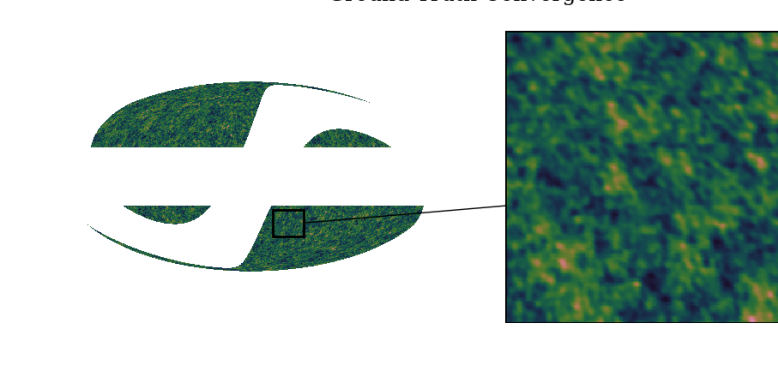
Figure 3: The top row displays the ground truth Takahashi convergence map as described in Section 5.1 with close up of a small region. Top to bottom: Increasing number density of galaxies ($n_{\text{gal}}$) and therefore decreasing noise levels. At the top we have $n_{\text{gal}}=5$ which is representative of current Stage iii@ surveys, at the bottom we have $n_{\text{gal}}=30$ which has been forecast for upcoming Stage iv@ surveys (e.g. Euclid / LSST). Left to right: The spherical Kaiser-Squires (Wallis et al., 2017a) estimator without the ad hoc smoothing kernel postprocessing, the optimally smoothed spheircal Kaiser-Squires estimator, and finally the DarkMapper estimator. Discussion: Clearly the DarkMapper estimator is visibly superior in all cases, numerically recovering both significantly larger SNR and Pearson correlation coefficients. All reconstructions have are plotted on the same colorscale to aid comparison (Green, 2011).

5.3 Reconstruction results

For an angular bandlimit $\ell_{\text{max}}=2048$, a pseudo-Euclid mask and input $n_{\text{gal}}\in[5,10,30,100]$ we compute the spherical Kaiser-Squires (SKS) estimator, an idealized (optimally smoothed) SKS estimator, and the DarkMapper estimator. The results can be found in Figure 3 and numerically in Table 1. In all cases the DarkMapper estimator provides the highest reconstruction fidelity both in terms of recovered SNR and Pearson correlation coefficient. Note that for $\ell_{\text{max}}=2048$ and the number density of galaxy observations selected the mean number of galaxies per pixel is $\mathcal{O}(10-10^{3})$.

It is important to note that the optimal smoothing kernel for the SKS estimator cannot be known and thus in practice is often selected ‘by eye’ which is to say selected ad hoc. Therefore the smoothed SKS results here constitute an upper bound. The DarkMapper framework is fully principled and requires no ad hoc parameter selection and is therefore likely to perform in much the same way when applied to observational data.

For Stage iii@ survey settings with $n_{\text{gal}}=5,10$ the increase in SNR ($\Delta$ SNR) of the DarkMapper estimator over the SKS (optimally smoothed SKS) estimator was $+15.286\;(+4.532)$ dB and $+14.093\;(+6.191)$ dB respectively. Recall that dB is measured on a logarithmic scale (see equation 43) and so this increase is quite dramatic. Furthermore the Pearson correlation coefficient increased from $0.403\;(0.759)$ to $0.904$ and $0.532\;(0.860)$ to $0.935$ for $n_{\text{gal}}=5,10$ respectively.

For the Stage iv@ Euclid-type setting with $n_{\text{gal}}=30$ $\Delta$, SNR was found to be $+11.858\;(+8.513)$ dB, along with which the Pearson correlation coefficient rose from $0.723\;(0.854)$ to $0.964$. As this setting is highly representative of the observations which will be made in Stage iv@ surveys this strongly suggests that algorithms such as DarkMapper should be adopted for weak lensing mass-mapping.

6 Application to public data

Finally we apply both the SKS and DarkMapper estimators to a collated map of the majority of the public wide field weak lensing observational datasets in order to reconstruct a single global dark-matter mass-map computed natively on the sphere. Furthermore we demonstrate straightforward global uncertainty quantification on our reconstruction.

Specifically we perform convergence reconstructions on the DESY1 (Abbott et al., 2018; Morganson et al., 2018; Flaugher et al., 2015), CFHTLens (Erben et al., 2012), and the KiDS450 (Hildebrandt et al., 2017; Fenech Conti et al., 2017) weak lensing shear datasets. See specific acknowledgements and related papers for further details. Note that throughout we have not chosen to perform reduced shear iterations, assuming that the observed shear is approximately the reduced shear $\gamma\sim g$ (in a more detailed analysis one could perform such further iterations)

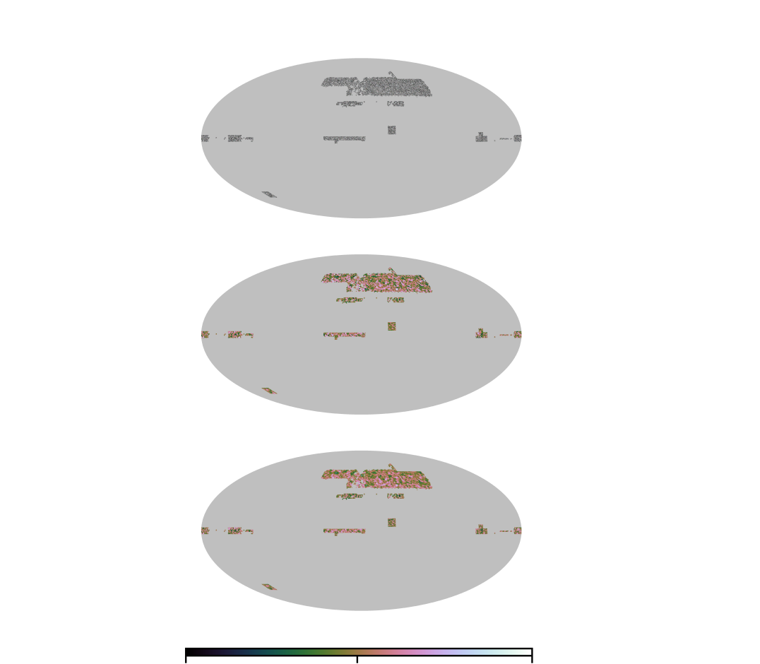
Figure 4: Mollweide projections of global reconstruction of the majority of public weak lensing datasets. Top to bottom: Spherical Kaiser-Squires (SKS) estimator without Gaussian smoothing kernel, SKS estimator with FWHM = $\Theta=25$ arcmin smoothing kernel (as in other studies), DarkMapper (our) estimator. All reconstructions are plotted on the same colorscale to aid comparison (Green, 2011). The data-sets can be found online at https://doi.org/10.5281/zenodo.3980652.

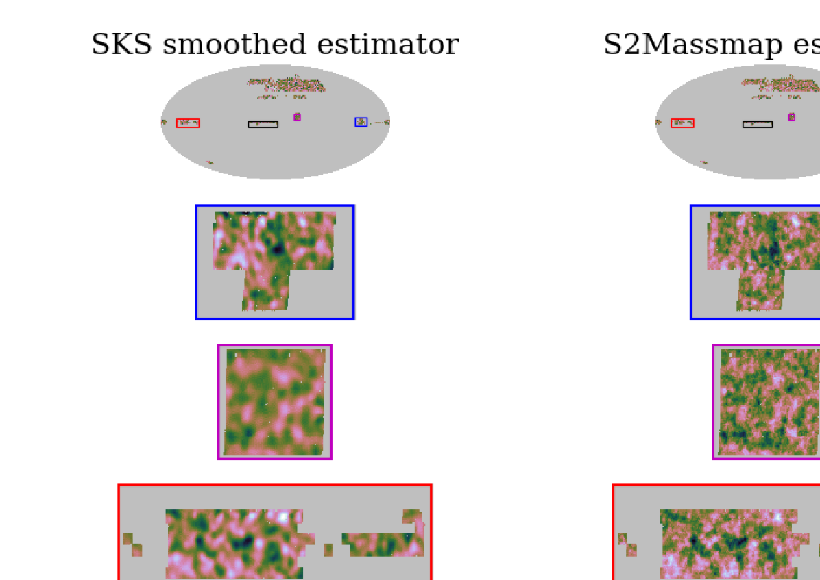
Figure 5: Top to bottom: Global reconstruction of the majority of public weak lensing datasets, magnified view of a variety of patches. Left to right: Spherical Kaiser-Squires (SKS) estimator without Gaussian smoothing kernel, SKS estimator with FWHM = $\Theta=25$ arcmin smoothing kernel (as in other studies), DarkMapper (our) estimator. Discussion: Note the overall agreement between both the smoothed SKS estimator and our DarkMapper estimator, however notice the significant increase in small-scale detail captured by the DarkMapper estimator. All reconstructions are plotted on the same colorscale to aid comparison (Green, 2011). These data-sets can be found online at https://doi.org/10.5281/zenodo.3980652.

6.1 Joint Spherical Mass-Map

All aforementioned weak lensing shear observational datasets were collated into a single joint global dataset. For each data-set we select only galaxies with non-zero catalog weight $w(i)>0$ and perform a correction for the multiplicative bias by $w(i)$ and additive by $c_{1,2}(i)$ biases per observation. Specifically this correction for ellipticities $e_{1,2}(i)$ is given by

$$\Re\{\gamma(i)\}=\frac{\sum_{j}w(j)\{e_{1}(j)-c_{1}(j)\}}{\sum_{j}w(j)\{1+\text{mcorr}(j)\}},$$

$$\Im\{\gamma(i)\}=\frac{\sum_{j}w(j)\{e_{2}(j)-c_{2}(j)\}}{\sum_{j}w(j)\{1+\text{mcorr}(j)\}},$$ (46)

where $j$ are observations such that observation $j$ belongs to pixel $i$, mcorr is the catalog magnification correction and $\Re,\Im$ denote the real and imaginary components of the shear field $\bm{\gamma}$ respectively.

This joint global dataset was then projected onto an equiangularly sampled (MW) spherical shear map $\gamma_{\text{obs}}$ with an angular bandlimit of $\ell_{\text{max}}=2048$. During this projection the number of galaxies projected into each pixel was recorded to create a complimentary map of observations per pixel, from which the data covariance $\Sigma_{\text{obs}}$ is directly determined (as discussed in Sections 3.2.1 and 5.2.1)

To this spherical shear map $\gamma_{\text{obs}}$ (with corresponding data covariance $\Sigma_{\text{obs}}$) we apply DarkMapper outlined in Section 3 with the same parameter choices outlined in Section 5 (see Price et al., 2018, for a planar equivalent). Additionally, we provide the SKS (Wallis et al., 2017a) reconstruction which we present in both its fundamental form (without post-processing Gaussian smoothing) and in its typical form (with post-processing Gaussian smoothing with full width at half maximum FWHM = $\Theta=25$ arcmins). All data products aforementioned within this section are publicly available and may be found at https://doi.org/10.5281/zenodo.3980652.

The results of all reconstruction algorithms can be seen globally in Figure 4 and with enhanced regions in Figure 5, where all subplots share the same colourscale (Green, 2011). It is immediately apparent that the SKS estimator, in the absence of smoothing, is overwhelming dominated by noise (hence the motivation for post-processing).

In contrast to this, the SKS estimator with a $\Theta=25$ arcmin post-processing Gaussian smoothing is largely in agreement with the DarkMapper estimator, however this smoothed SKS estimator unsurprisingly lacks any significant small-scale structure. Further note that the smoothed SKS estimator does not mirror all high intensity structure (e.g. peaks and voids) recovered by the DarkMapper estimator, which indicates more significant deviations between the two estimators. The most egregious of these cases is highlighted in the red boxed KiDS450 patch of Figure 5.

These structural dissimilarities between the smoothed SKS and DarkMapper estimator may reasonably be attributed to large noise fluctuations and boundary effects, both of which are not reasonably accounted for by the SKS estimator. Observation of such significant differences indicates that more principled reconstruction algorithms (such as DarkMapper) are important considerations when attempting to perform future statistical and scientific inference from dark matter mass-maps.

All reconstructions were performed on a 2016 MacBook air and took $\sim 30$ hours to compute. A further $\sim 100$ hours were optionally undertaken for annealing iterations to optimise the convergence. Note that this is by no means a benchmark of computational performance.

Surrogate $\kappa^{\text{sur}}$		Analysis ($\epsilon^{\prime}_{99\%}=842789$)		Hypothesis test
Estimator	$\Theta$ (arcmin)	Obj($\kappa^{\text{sur}}$)	Obj($\kappa^{\text{sur}})/\epsilon^{\prime}_{99\%}$	$\kappa^{\text{sur}}\in C^{\prime}_{99\%}$
SKS	0	6151070	7.298	✗
	5	2584510	3.067	✗
	10	891266	1.058	✗
	15	586741	0.696	✓
	20	513223	0.609	✓
	25	488887	0.580	✓
	30	478245	0.567	✓

Table 2: Description: Uncertainty quantification of convergence estimators and smoothing scales, in each case the convergence surrogate solution $\kappa^{\text{sur}}$ is defined by estimator (i.e. SKS) and Gaussian smoothing scale FWHM = $\Theta$ in arcmins. For each surrogate both the objective function and the ratio of the objective function to the level set threshold at $99\%$ confidence $\epsilon^{\prime}_{99\%}$ is presented. The right hand column indicates whether a given surrogate $\kappa^{\text{sur}}$ belongs to the credible set (and is therefore not rejected as a possible solution to the reconstruction). Shaded in red are solutions which are rejected by Bayesian hypothesis testings. Discussion: Clearly, the SKS estimator without smoothing is unequivically rejected, which is concurrant with the community’s intuition that smoothing is required for the SKS estimator to produce physically meaningful solutions. The minimal smoothing scale required for any SKS solution to not be rejected is $\Theta\sim 15$ arcminutes, therefore with a typical smoothing of $\Theta\in[25,30]$ arcmins the SKS solution belongs to the DarkMapper credible set and cannot be rejected at $99\%$ confidence (i.e. the two estimators are not necessarily conflicting). Nevertheless, the DarkMapper estimator contains greater fine-scale structure.

6.2 Local uncertainty quantification

Given significant structural dissimilarities between the SKS and DarkMapper convergence estimators we performed several hypothesis tests of local structure. Specifically we addressed the missing peaks observed in the smoothed SKS estimator of the lower (red) region of Figure 5 but not in the corresponding DarkMapper estimator. We did so by performing local hypothesis testing of structure as described in Section 4.2.1 (see Price et al., 2018, for more comprehensive details).

In all cases the hypothesis test of local structure could not reject the existance of such structure at reasonable confidence. This is unsurprising given the notably high noise level inherent to Stage iii@ weak lensing surveys (which reduces the magnitude of the objective function thus making the approximate level set threshold $\epsilon_{\alpha}^{\prime}$ more difficult to reach; see Section 4) and the extremely high dimensionality $\sim\mathcal{O}(10^{7})$ of the reconstruction (which directly increases the level set threshold $\epsilon_{\alpha}^{\prime}$ in equation 40).

6.3 Global uncertainty quantification

For high dimensional cases it is often more informative to consider global features of the reconstruction, as discussed in Section 4. A question one may wish to address is for which smoothing scales $\Theta$ does the SKS estimator provide solutions that are not in disagreement with the DarkMapper estimator at some well defined confidence.

To address this question within our global uncertainty quantification we consider the SKS estimator with a variety of Gaussian smoothing kernels, specifically $\Theta=5i$ for integer $i\in[0,6]$, which is to say a uniform sampling of different (in practice arbitrary) smoothing choices ranging from no smoothing (the basic SKS estimator) to the typically adopted case of $\Theta\sim 30$ arcmin smoothing. In this way we can directly address the question of which smoothing scales produces solutions $\kappa^{\text{sur}}(\Theta)$ belong to the DarkMapper approximate HPD-credible region $C_{\alpha}^{\prime}$ (are consistent with the DarkMapper estimator) and which solutions are unacceptable (i.e. those solutions which reject the null hypothesis that the surrogate is within the credible set) at $100(1-\alpha)\%$ confidence.

The results of this global uncertainty quantification (at $99\%$ confidence) can be found numerically in Table 2. Despite the high noise level present in the joint dataset, the uncertainty quantification technique is sensitive enough to reject the SKS estimator for $\Theta=0,5,10$ arcminutes, which is to say that these smoothing scales are in disagreement with the DarkMapper estimator at $99\%$ confidence and are unlikely to be physically meaningful. This provides statistically rigourous evidence for the community’s intuition that SKS estimators require considerable smoothing to be considered meaningful.

This raises an interesting point worth noting: the SKS estimator (by construction) locates solutions within $C^{\prime}_{\alpha}$ which exhibit relatively little small-scale structure, whereas the DarkMapper estimator locates solutions within $C^{\prime}_{\alpha}$ which retain significantly greater small-scale structure. Therefore, though the two solutions do not disagree at $100(1-\alpha)\%$ confidence, the DarkMapper estimator places relatively more probability on small-scale structures.

Note that if both estimators provided details of the HPD credible set then a stronger discussion of the relative cardinality of the intersection of both HPD credible sets could be used to quantify the level of statistical agreement. However, in this case the SKS estimator does not support a principled statistical interpretation and so can only justifiably be treated as a point estimate.

7 Conclusions

In this paper we have extended the previously presented (Price et al., 2018) sparse Bayesian reconstruction formalism to the spherical setting, resulting in a sparse spherical Bayesian mass-mapping algorithm which we refer to as DarkMapper. This algorithm is general and accomodates any log-concave posterior. In this paper we adopt a Laplace-type sparsity promoting wavelet prior with a multivariate Gaussian likelihood.

The DarkMapper mass-mapping algorithm was benchmarked against spherical Kaiser-Squires (Wallis et al., 2017a) in a variety of realistic weak lensing settings (ranging from Stage iii@ to future space based surveys) using the Takahashi (Takahashi et al., 2017) N-body simulations and a pseudo-Euclid masking. In all cases we perform analysis at a typically adopted angular bandlimit of $\ell_{\text{max}}=2048$. We do not consider intrinsic alignments in this paper, but highlight how they may be included should one wish it.

In all simulations the DarkMapper algorithm dramatically outperforms (in both recovered SNR and recovered Pearson correlation coefficient) the SKS estimator, even when artificially selecting the optimal SKS smoothing kernel (i.e. even when biasing our evaluation in favour SKS as strongly as possible).

We extend approximate Bayesian uncertainty quantification methods (Pereyra, 2017; Price et al., 2018, 2019b; Price et al., 2019a; Cai et al., 2018b; Repetti et al., 2018) to the spherical setting and explain how one may leverage these methods from local uncertainty quantification to general global (or aggregate) uncertainty quantification.

The DarkMapper estimator was applied to a joint observational shear dataset constructed by collating the majority of publicly available weak lensing data – specifically the DESY1 (Abbott et al., 2018; Morganson et al., 2018; Flaugher et al., 2015), CFHTLens (Erben et al., 2012), and the KiDS450 (Hildebrandt et al., 2017; Fenech Conti et al., 2017) surveys. To the best of our knowledge this is the first joint spherical reconstruction of all public weak lensing shear observations.

For comparison we also computed the SKS estimator of this joint dataset. We find, as with the simulated benchmarking, that the DarkMapper algorithm recovers significantly more fine-scale structure without the need for any assumptions of Gaussianity or ad hoc smoothing parameters (i.e. the smoothing scale for SKS post-processing). This demonstrates that the algorithm works as expected on observational data.

Finally, uncertainty quantification was carried out to determine for which smoothing scales the SKS point estimates provide solutions that are acceptable solutions to the DarkMapper Bayesian inference problem (i.e. within the highest posterior density credible region) – this is to say the smoothing scales at which both convergence estimates are not conflicting at $99\%$ confidence. It was found that all SKS reconstructions with smoothing scales below $\sim 15$ arcmin were rejected at $99\%$ confidence, indicating that significant smoothing is required for agreement between the SKS and DarkMapper estimators. This reaffirms the community’s understanding that SKS estimators must undergo significant smoothing to recover physically meaningful convergence maps.

Moreover, we demonstrate that the DarkMapper estimator locates permissible solutions with significantly greater small-scale structure than those which are located by the SKS estimator. More constraining statistical statements were limited by the inherently high noise level in current observational shear data.

With the advent of Stage iv@ surveys the pixel noise level is projected to drop dramatically (due to increased galaxy number density), which will inevitably facilitate significantly more constraining statistical statements. As the DarkMapper estimator not only provides dramatically increased reconstruction fidelity over the SKS estimator but also supports a principled Bayesian interpretation, it will be of important use for application to Stage iv@ datasets.

Note that just as we have extended this sparse hierarchical Bayesian mass-mapping formalism to the sphere ($\mathbb{S}^{2}$) one can extend it to the ball ($\mathbb{B}^{3}$) and thus recover similar results for the case of full 3D mass-mapping. This is a possible avenue for future investigation.

8 Data Availability

All observational data utilized throughout this paper is publicly available and can be found in the corresponding references. All joint reconstruction data-sets are publicly available and can be found online at https://doi.org/10.5281/zenodo.3980652. The DarkMapper reconstruction software will be publicly released in the near future.

Appendix A Wavelets on the Sphere

This section will provide extremely brief (and quite technical) overview of scale-discretised spherical wavelets; for extensive details see the related articles (Wiaux et al., 2008; Wallis et al., 2017b; McEwen et al., 2015b, 2013a; Leistedt et al., 2013b; McEwen et al., 2015a; McEwen & Price, 2015; Chan et al., 2017a; McEwen et al., 2018).

The scale-discretized wavelet transform on the sphere is given by the directional convolution of each wavelet $\Psi^{j}$ of scale $j\in[J_{0},J_{\text{max}}]$ with a field ${}_{0}\kappa$, such that the wavelet coefficients $w^{j}(\rho)\in\ell_{\text{max}}^{2}(\text{SO}(3))$ are given by,

$$w^{j}(\rho)=\int_{\mathbb{S}^{2}}d\rho(\rho^{\prime})\;{}_{0}\kappa(\rho^{\prime})(\mathcal{R}_{\rho}\Psi^{j})^{*}(\rho^{\prime}).$$ (47)

Additionally, the low frequency component of ${}_{0}\kappa$ is encapsulated by the axisymmetric convolution with $\Upsilon\in\ell_{\text{max}}^{2}(\mathbb{S}^{2})$ such that,

$$s(\omega)=\int_{\mathbb{S}^{2}}d\Omega(\omega^{\prime})\;{}_{0}\kappa(\omega^{\prime})(\mathcal{R}_{\omega}\Upsilon)^{*}(\omega^{\prime}).$$ (48)

It is possible to project these directional and axisymmetric convolution operators into harmonic space (Wallis et al., 2017b),

$$(w^{j})^{\ell}_{mn}\equiv\langle w^{j},\mathcal{D}^{\ell*}_{mn}\rangle=\frac{8\pi^{2}}{2\ell+1}\;{}_{0}\kappa_{lm}\;\Psi^{j*}_{\ell n},$$ (49)

$$s_{\ell m}\equiv\langle s,Y_{\ell m}\rangle=\sqrt{\frac{4\pi}{2\ell+1}}\;{}_{0}\kappa_{lm}\;\Upsilon^{*}_{\ell 0}.$$ (50)

The coefficients of a general spherical signal ${}_{s}f$ can synthesised exactly by

$${}_{s}f(\omega)=\int_{\mathbb{S}^{2}}d\Omega s(\omega^{\prime})(\mathcal{R}_{\omega^{\prime}}s)(\omega^{\prime})+\sum_{j=J_{0}}^{J}\int_{\text{SO}(3)}d\rho w^{j}(\rho^{\prime})(\mathcal{R}_{\rho^{\prime}}w^{j})(\rho^{\prime}),$$ (51)

from which we can define the discretized form of ${}_{0}\kappa$ by

$${}_{0}\kappa(\omega)=\sum^{\infty}_{\ell=0}\sum^{\ell}_{m=-\ell}\Bigg{\{} \sqrt{\frac{4\pi}{2\ell+1}}s_{\ell m}\Upsilon_{\ell 0}Y_{\ell m}(\omega)$$

$$+\frac{2\ell+1}{8\pi^{2}}\sum_{j=J_{0}}^{J_{\text{max}}}\sum_{n=-\ell}^{\ell}(w^{j})^{\ell}_{mn}\;\Psi^{j}_{\ell n}Y_{\ell m}(\omega)\Bigg{\}},$$ (52)

where the harmonic coefficients ${}_{0}\kappa_{\ell m}$ are explicitly given by

$${}_{0}\kappa_{\ell m}=\sqrt{\frac{2\ell+1}{4\pi}}s_{\ell m}\Upsilon_{\ell 0}+\frac{2\ell+1}{8\pi^{2}}\sum_{j=J_{0}}^{J_{\text{max}}}\sum_{n=-\ell}^{\ell}(w^{j})^{\ell}_{mn}\;\Psi^{j}_{\ell n}$$ (53)

Combining equations (49) and (50) the harmonic representation of the spherical wavelet transform at scale $j$ can be written as a combination of the following linear operators (Wallis et al., 2017b):

$$\hat{w}^{j}=\bm{\mathsf{N}}^{j}\bm{\mathsf{W}}^{j}\;{}_{0}\hat{\kappa}_{\ell m},$$

are the Wigner coefficients of the directional wavelet coefficients. Here $\bm{\mathsf{W}}^{j}$ is harmonic space multiplication by the wavelet kernel $\Psi^{j*}_{\ell n}$, and $\bm{\mathsf{N}}^{j}$ corresponds to wavelet normalization.

$$\hat{s}=\bm{\mathsf{S}}\;{}_{0}\hat{\kappa}_{\ell m},$$

are the spherical harmonic coefficients of the scaling wavelet coefficients, where $\bm{\mathsf{S}}$ is harmonic space multiplication by scaling kernel $\Upsilon^{*}_{\ell 0}$.

We further specialize by grouping the harmonic representation of the coefficients into $\hat{\alpha}=\bm{\mathsf{N}}\bm{\mathsf{W}}\;{}_{0}\hat{\kappa}_{\ell m},$ where the wavelet scale normalization terms are collectively $\bm{\mathsf{N}}=\text{diag}(\mathbb{I},\bm{\mathsf{N}}^{J_{0}},\ldots,\bm{\mathsf{N}}^{J_{\text{max}}}),$ and the Wigner/harmonic space wavelet convolutions are collectively $\bm{\mathsf{W}}=\text{diag}(\bm{\mathsf{S}},\bm{\mathsf{W}}^{J_{0}},\ldots,\bm{\mathsf{W}}^{J_{\text{max}}}).$ Finally we introduce a diagonal array of operators $\bm{\mathsf{H}}$ corresponding to inverse spherical harmonic and Wigner transforms, $\bm{\mathsf{H}}=\text{diag}(\bm{\mathsf{Y}},\bm{\mathsf{\mathcal{D}}}^{J_{0}},\ldots,\bm{\mathsf{\mathcal{D}}}^{J_{\text{max}}})$ In the scope of this paper we restrict ourselves to the analysis setting, thus these are the only operators required though a complete set are provided in Wallis et al. (2017b). Concatenating these operators we can finally form analysis forward and adjoint wavelet transforms,

$$\tilde{\Psi}=\bm{\mathsf{H}}\bm{\mathsf{N}}\bm{\mathsf{W}}\tilde{\bm{\mathsf{Y}}}\qquad\text{and}\qquad\tilde{\Psi}^{\dagger}=\tilde{\bm{\mathsf{Y}}}^{\dagger}\bm{\mathsf{W}}^{\dagger}\bm{\mathsf{N}}\bm{\mathsf{H}}^{\dagger}.$$ (54)

Note that $\dagger$ is the adjoint (or conjugate transpose) operator, and as $\bm{\mathsf{N}}$ is simply wavelet scaling it is trivially self-adjoint $\bm{\mathsf{N}}=\bm{\mathsf{N}}^{\dagger}$. Crucially as we work in the discrete setting the inverse wavelet transforms are not equivalent to the adjoint wavelet transforms, and so we adopt the optimized algorithms to compute fast Wigner and Wigner adjoint functions presented in the appendix of McEwen et al. (2015b).

References

- Abbott et al. (2018) Abbott T. M. C., et al., 2018, ApJS, 239, 18
- Alsing et al. (2015) Alsing J., Kirk D., Heavens A., Jaffe A. H., 2015, MNRAS, 452, 1202
- Alsing et al. (2016) Alsing J., Heavens A., Jaffe A. H., Kiessling A., Wandelt B., Hoffmann T., 2016, MNRAS, 455, 4452
- Baldi et al. (2009) Baldi P., Kerkyacharian G., Marinucci D., Picard D., et al., 2009, The Annals of Statistics, 37, 1150
- Barreiro et al. (2000) Barreiro R. B., Hobson M. P., Lasenby A. N., Banday A. J., Górski K. M., Hinshaw G., 2000, MNRAS, 318, 475
- Bartelmann & Schneider (2001) Bartelmann M., Schneider P., 2001, Phys. Rep., 340, 291
- Bunn et al. (2003) Bunn E. F., Zaldarriaga M., Tegmark M., de Oliveira-Costa A., 2003, Phys. Rev. D, 67, 023501
- Cai et al. (2018a) Cai X., Pereyra M., McEwen J. D., 2018a, MNRAS, 480, 4154
- Cai et al. (2018b) Cai X., Pereyra M., McEwen J. D., 2018b, MNRAS, 480, 4170
- Carrillo et al. (2012) Carrillo R. E., McEwen J. D., Wiaux Y., 2012, MNRAS, 426, 1223
- Carrillo et al. (2013) Carrillo R. E., McEwen J. D., Van De Ville D., Thiran J.-P., Wiaux Y., 2013, IEEE Signal Processing Letters, 20, 591
- Castro et al. (2005) Castro P. G., Heavens A. F., Kitching T. D., 2005, Phys. Rev. D, 72, 023516
- Chan et al. (2017a) Chan J. Y. H., Leistedt B., Kitching T. D., McEwen J. D., 2017a, IEEE Transactions on Signal Processing, 65, 5
- Chan et al. (2017b) Chan J. Y. H., Leistedt B., Kitching T. D., McEwen J. D., 2017b, IEEE Transactions on Signal Processing, 65, 5
- Chang et al. (2018) Chang C., et al., 2018, MNRAS, 475, 3165
- Clowe et al. (2006) Clowe D., Brada M., Gonzalez A. H., Markevitch M., Randall S. W., Jones C., Zaritsky D., 2006, ApJ, 648, L109
- Coles & Chiang (2000) Coles P., Chiang L.-Y., 2000, Nature, 406, 376
- Combettes & Pesquet (2009) Combettes P. L., Pesquet J.-C., 2009, preprint, (arXiv:0912.3522)
- Corless et al. (2009) Corless V. L., King L. J., Clowe D., 2009, MNRAS, 393, 1235
- Erben et al. (2012) Erben T., et al., 2012, Monthly Notices of the Royal Astronomical Society, 433
- Erben et al. (2013) Erben T., et al., 2013, MNRAS, 433, 2545
- Fenech Conti et al. (2017) Fenech Conti I., Herbonnet R., Hoekstra H., Merten J., Miller L., Viola M., 2017, MNRAS, 467, 1627
- Flaugher et al. (2015) Flaugher B., et al., 2015, AJ, 150, 150
- Fluri et al. (2018) Fluri J., Kacprzak T., Sgier R., Refregier A., Amara A., 2018, J. Cosmology Astropart. Phys., 2018, 051
- Fluri et al. (2019) Fluri J., Kacprzak T., Lucchi A., Refregier A., Amara A., Hofmann T., Schneider A., 2019, Phys. Rev. D, 100, 063514
- Giblin et al. (2018) Giblin B., et al., 2018, Monthly Notices of the Royal Astronomical Society, 480, 5529
- Goldberg et al. (1967) Goldberg J. N., Macfarlane A. J., Newman E. T., Rohrlich F., Sudarshan E. C. G., 1967, Journal of Mathematical Physics, 8, 2155
- Green (2011) Green D. A., 2011, Bulletin of the Astronomical Society of India, 39, 289
- Grimm & Yoo (2018) Grimm N., Yoo J., 2018, J. Cosmology Astropart. Phys., 2018, 067
- Hildebrandt et al. (2017) Hildebrandt H., et al., 2017, MNRAS, 465, 1454
- Hinshaw et al. (2013) Hinshaw G., et al., 2013, ApJS, 208, 19
- Horowitz et al. (2018) Horowitz B., Seljak U., Aslanyan G., 2018, arXiv preprint arXiv:1810.00503
- Jee et al. (2016) Jee M. J., Dawson W. A., Stroe A., Wittman D., van Weeren R. J., Brüggen M., Bradač M., Röttgering H., 2016, ApJ, 817, 179
- Jeffrey et al. (2018) Jeffrey N., et al., 2018, MNRAS, 479, 2871
- Kaiser & Squires (1993) Kaiser N., Squires G., 1993, ApJ, 404, 441
- Kuijken et al. (2015) Kuijken K., et al., 2015, MNRAS, 454, 3500
- Lanusse et al. (2016) Lanusse F., Starck J.-L., Leonard A., Pires S., 2016, A&A, 591, A2
- Laureijs et al. (2011) Laureijs R., et al., 2011, arXiv e-prints, p. arXiv:1110.3193
- Leistedt et al. (2013a) Leistedt B., McEwen J. D., Vandergheynst P., Wiaux Y., 2013a, A&A, 558, A128
- Leistedt et al. (2013b) Leistedt B., McEwen J. D., Vandergheynst P., Wiaux Y., 2013b, A&A, 558, A128
- Mallat (1999) Mallat S., 1999, A Wavelet Tour of Signal Processing
- Marinucci et al. (2007) Marinucci D., et al., 2007, Monthly Notices of the Royal Astronomical Society, 383, 539
- McEwen & Price (2015) McEwen J. D., Price M. A., 2015, arXiv e-prints, p. arXiv:1510.01595
- McEwen & Price (2019) McEwen J. D., Price M. A., 2019, in 27th European Signal Processing Conference (EUSIPCO). (arXiv:1510.01595)
- McEwen & Scaife (2008) McEwen J. D., Scaife A. M. M., 2008, MNRAS, 389, 1163
- McEwen & Wiaux (2011) McEwen J. D., Wiaux Y., 2011, IEEE Transactions on Signal Processing, 59, 5876
- McEwen et al. (2011) McEwen J. D., Wiaux Y., Eyers D. M., 2011, A&A, 531, A98
- McEwen et al. (2013a) McEwen J. D., Puy G., Thiran J.-P., Vandergheynst P., Van De Ville D., Wiaux Y., 2013a, IEEE Transactions on Image Processing, 22, 2275
- McEwen et al. (2013b) McEwen J. D., Vandergheynst P., Wiaux Y., 2013b, in Proc. SPIE. p. 88580I (arXiv:1308.5706), doi:10.1117/12.2022889
- McEwen et al. (2015a) McEwen J. D., Leistedt B., Büttner M., Peiris H. V., Wiaux Y., 2015a, preprint, (arXiv:1509.06749)
- McEwen et al. (2015b) McEwen J. D., Buttner M., Leistedt B., Peiris H. V., Wiaux Y., 2015b, IEEE Signal Processing Letters, 22, 2425
- McEwen et al. (2018) McEwen J. D., Durastanti C., Wiaux Y., 2018, Applied and Computational Harmonic Analysis, 44, 59
- McFarland et al. (2013) McFarland J. P., Verdoes-Kleijn G., Sikkema G., Helmich E. M., Boxhoorn D. R., Valentijn E. A., 2013, Experimental Astronomy, 35, 45
- Mediavilla et al. (2016) Mediavilla E., Muñoz J. A., Garzón F., Mahoney T. J., 2016, Astrophysical Applications of Gravitational Lensing
- Miller et al. (2013) Miller L., et al., 2013, MNRAS, 429, 2858
- Moreau (1962) Moreau J. J., 1962, C.R. Acad. Sci. Paris Ser. A Math., 255, 2897
- Morganson et al. (2018) Morganson E., et al., 2018, PASP, 130, 074501
- Munshi & Coles (2017) Munshi D., Coles P., 2017, J. Cosmology Astropart. Phys., 2, 010
- Narcowich et al. (2006) Narcowich F. J., Petrushev P., Ward J. D., 2006, SIAM Journal on Mathematical Analysis, 38, 574
- Newman & Penrose (1966) Newman E. T., Penrose R., 1966, Journal of Mathematical Physics, 7, 863
- Onose et al. (2016) Onose A., Carrillo R. E., Repetti A., McEwen J. D., Thiran J.-P., Pesquet J.-C., Wiaux Y., 2016, MNRAS, 462, 4314
- Peel et al. (2018) Peel A., Pettorino V., Giocoli C., Starck J.-L., Baldi M., 2018, A&A, 619, A38
- Pereyra (2017) Pereyra M., 2017, SIAM Journal on Imaging Sciences, 10, 285
- Pereyra et al. (2015) Pereyra M., Bioucas-Dias J., Figueiredo M., 2015, Maximum-a-posteriori estimation with unknown regularisation parameters. pp 230–234, doi:10.1109/EUSIPCO.2015.7362379
- Pichon et al. (2010) Pichon C., Thiébaut E., Prunet S., Benabed K., Colombi S., Sousbie T., Teyssier R., 2010, MNRAS, 401, 705
- Planck Collaboration et al. (2018) Planck Collaboration et al., 2018, arXiv preprint arXiv:1807.06209
- Pratley et al. (2018) Pratley L., McEwen J. D., d’Avezac M., Carrillo R. E., Onose A., Wiaux Y., 2018, MNRAS, 473, 1038
- Price et al. (2018) Price M. A., Cai X., McEwen J. D., Kitching T. D., Wallis C. G. R., 2018, submitted to MNRAS
- Price et al. (2019a) Price M. A., McEwen J. D., Cai X., Kitching T. D., 2019a, Monthly Notices of the Royal Astronomical Society, 489, 3236
- Price et al. (2019b) Price M. A., Cai X., McEwen J. D., Pereyra M., Kitching T. D., 2019b, Monthly Notices of the Royal Astronomical Society, 492, 394
- Price et al. (2020) Price M. A., Pratley L., McEwen J. D., 2020, in prep
- Repetti et al. (2018) Repetti A., Pereyra M., Wiaux Y., 2018, preprint, (arXiv:1803.00889)
- Robert (2001) Robert C.-P., 2001, The Bayesian Choice, doi:https://doi.org/10.1007/0-387-71599-1.
- Schneider (2005) Schneider P., 2005, ArXiv Astrophysics e-prints,
- Schneider et al. (2015) Schneider M. D., Hogg D. W., Marshall P. J., Dawson W. A., Meyers J., Bard D. J., Lang D., 2015, ApJ, 807, 87
- Schröder & Sweldens (1995) Schröder P., Sweldens W., 1995, in Computer Graphics Proceedings (SIGGRAPH ‘95). pp 161–172
- Starck et al. (2006) Starck J.-L., Moudden Y., Abrial P., Nguyen M., 2006, Astronomy & Astrophysics, 446, 1191
- Takahashi et al. (2017) Takahashi R., Hamana T., Shirasaki M., Namikawa T., Nishimichi T., Osato K., Shiroyama K., 2017, ApJ, 850, 24
- Taylor et al. (2018) Taylor P. L., Kitching T. D., McEwen J. D., 2018, Phys. Rev. D, 98, 043532
- Trotta (2017) Trotta R., 2017, preprint, (arXiv:1701.01467)
- Vallis et al. (2018) Vallis Z. M., Wallis C. G. R., Kitching T. D., 2018, Astronomy and Computing, 24, 84
- Van Waerbeke et al. (2013) Van Waerbeke L., et al., 2013, MNRAS, 433, 3373
- VanderPlas et al. (2011) VanderPlas J. T., Connolly A. J., Jain B., Jarvis M., 2011, ApJ, 727, 118
- Wallis et al. (2017a) Wallis C. G. R., McEwen J. D., Kitching T. D., Leistedt B., Plouviez A., 2017a, preprint, (arXiv:1703.09233)
- Wallis et al. (2017b) Wallis C. G. R., Wiaux Y., McEwen J. D., 2017b, IEEE Transactions on Image Processing, 26, 5176
- Wiaux et al. (2008) Wiaux Y., McEwen J. D., Vandergheynst P., Blanc O., 2008, MNRAS, 388, 770
- de Jong et al. (2015) de Jong J. T. A., et al., 2015, A&A, 582, A62