Dirac Particles in Transparent Quantum Graphs:
Tunable transport of relativistic quasiparticles in branched structures

Abstract

We consider the dynamics of relativistic spin-half particles in quantum graphs with transparent branching points. The system is modeled by combining the quantum graph concept with the one of transparent boundary conditions applied to the Dirac equation on metric graphs. Within such an approach, we derive simple constraints, which turn the usual Kirchhoff-type boundary conditions at the vertex equivalent to the transparent ones. Our method is applied to quantum star graph. An extension to more complicated graph topologies is straightforward.

I Introduction

Due to the recent development in condensed matter physics, modeling of relativistic particle dynamics in low-dimensional systems attracted much attention. It has been discovered that such materials as graphene Neto ; Kotov ; BF , carbon nanotubes (CNT) CNT , topological insulators TI1 ; TI2 , and some types of superconductors Jackiw ; Alicea1 , can provide quasiparticle excitations, which can mimic relativistic dynamics. Such quasiparticles are described in terms of the Dirac, Weyl and Bogoliubov de Gennes equations. Low dimensional functional materials, in which such quasiparticles appear, can be used for engineering of different nanoscale electronic and optoelectronic devices in emerging quantum technologies.

Effective functionalization and device optimization in such technologies require solving the problem of tunable particle transport in low-dimensional structures. Subsequently, this requires developing effective and realistic models for the relativistic quasiparticle transport in low-dimensional systems. As most of the low-dimensional systems, arising in condensed matter, exhibit a branched structure, the above task can be reduced to the problem of relativistic quasiparticle dynamics modeling in branched quantum systems. These latter mentioned are usually modeled in terms of so-called quantum graphs, which has attracted much attention during past three decades (see, Refs. Uzy1 ; Hul ; Kuchment04 ; Uzy2 ; Exner15 for review recent developments in this research field).

In this paper we consider the problem of transparent quantum graphs for relativistic (spin-half) quasiparticles described in terms of the Dirac equation on metric graphs. The model we propose can be directly applied to the problem of tunable transport of relativistic quasiparticles in branched graphene nanoribbons, carbon nanoribbon networks, topological insulator networks and branched optical fibers, where the Dirac quasiparticles appear. Combining quantum graph and transparent boundary conditions concepts, we derive explicit vertex boundary conditions, providing reflectionless transport of quasiparticles through the branching points. We reveal simple constraints for the regime, when the motion of relativistic spin-half quasiparticle in quantum graph becomes reflectionless, i.e., the quantum graph becomes transparent with respect to the particle transport.

The motivation for the study of transparent quantum graphs arises from the wide range of practical applications in optoelectronics and condensed matter physics. Effective signal transfer in optoelectronic networks requires a reduction to minimum losses. Spin, charge and energy transport in branched nanomaterials used in nanoelectronic devices also requires minimization of losses caused by backscattering of quasiparticles. In the context of relativistic quantum dynamics with reflectionless transport, this problem will appear in low-dimensional functional materials (e.g., graphene, CNT, topological insulators, one-dimensional branched quasimolecules, etc). Different quantum wire networks appearing in solid state physics are also potential structures, where the wave transport can be tuned from the diffusive to the ballistic regime using transparent boundary conditions.

The paper is organized as follows. In the next section we give a brief description of the transparent boundary conditions for the Dirac equation on a real line. Section III presents a short introduction to the Dirac equation on quantum graphs. Section IV includes our study of Dirac particles in transparent quantum graphs. A numerical justification of the obtained results is stated in Section V. Finally, Section VI concludes our work with some final remarks.

II Transparent boundary conditions for the Dirac equation on a line

The standard way for the description of particle and wave scattering in quantum mechanics is the scattering matrix based approach. However, within such an approach one does not use explicit solutions of the Schrödinger equation and hence, it is less effective for the cases, when one needs to describe the transmission of the wave through the boundary of two domains. Moreover, it does not provide any solution for the problem of tunable scattering and transmission of particles for a given point/domain using the initial conditions for the Schrödinger equation.

An effective approach providing solutions of the problem of reflectionless transmission of the waves and particles through the given point/boundary in terms of a Cauchy problem has attracted much attention during the past three decades. Within such an approach, one can formulate boundary conditions for the absence of backscattering at a given point or domain boundary, although the explicit form of such boundary conditions are much more complicated than those of Dirichlet, Neumann and Robin conditions. Such boundary conditions are called transparent boundary conditions (TBCs).

A TBC is a boundary condition for a wave-type equation, which leads to a solution providing minimum (or absence) of reflections. In early works (see, e.g., EM1 ; EM2 ; Halpern ; Sofronov ; Shibata ; Kuska ) the TBC was defined as a boundary conditions providing a minimum of backscattering in terms of the reflection coefficient. However, later a more strict mathematical definition of a TBC has been provided as follows Arnold1998 ; Ehrhardt1999 ; Ehrhardt2001 ; Ehrhardt2002 ; Arnold2003 ; Jiang2004 ; Antoine2008 ; Ehrhardt2008 ; Sumichrast2009 ; Antoine2009 ; Ehrhardt2010 ; Klein2011 ; Arnold2012 ; Feshchenko2013 ; Antoine2014 . For a given finite domain, $\Omega$, the TBCs are imposed in such a way that the solution of a PDE in $\Omega$ corresponds to that in the whole space, i.e., the wave/particle moving inside/outside the domain does not ‘see’ the boundary of the domain. The construction of the TBC is based on the coupling of initial value boundary problems (IVBPs) in interior and exterior domains Arnold1998 ; Ehrhardt1999 ; Ehrhardt2001 ; Ehrhardt2002 ; Arnold2003 ; Jiang2004 ; Antoine2008 ; Ehrhardt2008 ; Sumichrast2009 ; Antoine2009 ; Ehrhardt2010 ; Klein2011 ; Arnold2012 ; Feshchenko2013 ; Antoine2014 .

The general procedure for constructing transparent boundary conditions on a real line here reads as follows, cf. Antoine2008

1. Split the original PDE evolution problem into coupled equations: the interior and exterior problems.

2. Apply a Laplace transformation to exterior problems on $\Omega^{\rm ext}$.

3. Solve (explicitly, numerically) the ordinary differential equations in the spatial unknown $x$.

4. Allow only “outgoing” waves by selecting the decaying solution as $x\to\pm\infty$.

5. Match Dirichlet and Neumann values at the artificial boundary.

6. Apply (explicitly, numerically) the inverse Laplace transformation.

Especially, in case of the Dirac equation this recipe above was applied by Hammer, W. Pötz and Arnold Hammer2014 in order to derive (continuous) TBCs, cf. Eq. (13).

The early treatment of the problem of transparent boundary conditions in terms of the acoustic wave equation dates back to the pioneering work of Engquist and Majda EM1 ; EM2 . The further development of the concept of TBCs for some parabolic and hyperbolic PDEs was presented by Halpern Halpern and Sofronov Sofronov . A more comprehensive study of TBCs for the Schrödinger equation and other wave equation can be found in Arnold1998 ; Ehrhardt1999 ; Ehrhardt2001 ; Ehrhardt2002 ; Arnold2003 ; Jiang2004 ; Antoine2008 ; Ehrhardt2008 ; Sumichrast2009 ; Antoine2009 ; Ehrhardt2010 ; Klein2011 ; Arnold2012 ; Feshchenko2013 ; Antoine2014 ; Petrov2016 . Earlier, approximate TBCs for the linear Schrödinger equation were formulated by Shibata Shibata and Kuska Kuska , where the dispersion relations for the plane waves are approximated in order to derive approximative TBCs. A strict mathematical analysis of TBCs for different wave equations, including the quantum mechanical Schrödinger equation can be found in the Refs. Ehrhardt2002 ; Arnold2003 ; Ehrhardt2008 ; Antoine2014 ; Petrov2016 . Here we briefly recall the formulation of TBCs on a line following the Refs. Ehrhardt1999 ; Ehrhardt2001 ; Ehrhardt2002 ; Arnold2003 .

Before proceeding to transparent quantum graphs, following the Ref. Hammer2014 , we briefly present the concept of TBCs for the Dirac equation. We consider the following Dirac equation (in units $\hbar=c=1$) posed on an interval $[0,L]\subset\mathbb{R}$:

$$\begin{split}i\partial_{t}\phi&=-i\partial_{x}\chi+m\phi,\\ i\partial_{t}\chi&=-i\partial_{x}\phi-m\chi.\end{split}$$ (1)

The initial conditions for Eq. (1) are imposed as

$$\phi(x,0)=\phi^{I}(x),\quad\chi(x,0)=\chi^{I}(x),\quad x\in[0,L].$$ (2)

Further, we divide the entire space into interior ($0<x<L$) and two exterior ($x\leq 0$ and $x\geq L$) domains. Then, the interior problem ($x\in(0,L)$, $t>0$) reads

$$\begin{split}i\partial_{t}\phi&=-i\partial_{x}\chi+m\phi,\\ i\partial_{t}\chi&=-i\partial_{x}\phi-m\chi,\\ \phi(x,0)&=\phi^{I}(x),\\ \chi(x,0)&=\chi^{I}(x),\\ (T_{0}\phi)(0,t)&=\chi(0,t),\\ (T_{L}\phi)(L,t)&=\chi(L,t),\end{split}$$ (3)

where $T_{0}$ and $T_{L}$ denote the Dirichlet–to–Neumann (DtN) maps at the boundaries, and they are found by solving the exterior problems ($x\leq 0$ and $x\geq L$, $t>0$) given as

$$\begin{split}i\partial_{t}\phi&=-i\partial_{x}\chi+m\phi,\\ i\partial_{t}\chi&=-i\partial_{x}\phi-m\chi,\\ \phi(x,0)&=0,\\ \chi(x,0)&=0,\\ \phi(0,t)&=\Phi_{1}(t),\\ \chi(0,t)&=(T_{0}\phi)(0,t),\\ \phi(L,t)&=\Phi_{2}(t),\\ \chi(L,t)&=(T_{L}\phi)(L,t).\end{split}$$ (4)

By introducing the following Laplace transformations

$$\widetilde{\phi}(x,s) =\int_{0}^{+\infty}\phi(x,t)\,e^{-st}\,dt,$$ (5)

$$\widetilde{\chi}(x,s) =\int_{0}^{+\infty}\chi(x,t)\,e^{-st}\,dt,$$ (6)

one can rewrite Eq. (1) as ordinary differential equations

$$\begin{split}-i\partial_{x}\widetilde{\chi}(x,s)&=(is-m)\widetilde{\phi}(x,s),\\ -i\partial_{x}\widetilde{\phi}(x,s)&=(is+m)\widetilde{\chi}(x,s).\end{split}$$ (7)

The general solution of the system (7) can be written as

$$\begin{split}&\widetilde{\phi}(x,s)=c_{1}\,e^{-\sqrt[+]{s^{2}+m^{2}}x}+c_{2}\,e^{\sqrt[+]{s^{2}+m^{2}}x},\\ &\widetilde{\chi}(x,s)=-c_{1}\kappa\,e^{-\sqrt[+]{s^{2}+m^{2}}x}+c_{2}\kappa\,e^{\sqrt[+]{s^{2}+m^{2}}x},\end{split}$$ (8)

where $\kappa=\frac{\sqrt[+]{is-m}}{\sqrt[+]{is+m}}$. Since we require $\widetilde{\phi}$, $\widetilde{\chi}\in L_{2}(0,+\infty)$, we obtain for $x\geq L$ (right exterior domain) the condition $c_{1}=0$, and thus

$$\begin{split}\widetilde{\phi}(x,s)&=c_{2}\,e^{\sqrt[+]{s^{2}+m^{2}}x},\\ \widetilde{\chi}(x,s)&=c_{2}\kappa\,e^{\sqrt[+]{s^{2}+m^{2}}x}.\end{split}$$ (9)

From the initial condition of the problem (4) we obtain

$$c_{2}=\widetilde{\phi}(L,s)e^{-\sqrt[+]{s^{2}+m^{2}}L}=\widetilde{\Phi}_{2}(s)e^{-\sqrt[+]{s^{2}+m^{2}}L},$$

hence

$$\begin{split}\widetilde{\phi}(x,s)&=\widetilde{\Phi}_{2}(s)\,e^{\sqrt[+]{s^{2}+m^{2}}(x-L)},\\ \widetilde{\chi}(x,s)&=\widetilde{\Phi}_{2}(s)\kappa\,e^{\sqrt[+]{s^{2}+m^{2}}(x-L)}=\kappa\widetilde{\phi}(x,s).\end{split}$$ (10)

Thus, one gets finally

$$\widetilde{\chi}(L,s)=\kappa\widetilde{\phi}(L,s).$$ (11)

Using the inverse Laplace transformation we have

$$\begin{split}\chi(L,t)=&\frac{d}{dt}\int_{0}^{t}I_{0}\bigl{(}m(t-\tau)\bigr{)}\phi(L,\tau)\,d\tau\\ &+im\int_{0}^{t}I_{0}\bigl{(}m(t-\tau)\bigr{)}\phi(L,\tau)\,d\tau,\end{split}$$ (12)

where $I_{0}(z)$ denotes the modified Bessel function. Analogously, one can get the TBC at $x=0$ Hammer2014 :

$$\begin{split}\chi(0,t)=&-\frac{d}{dt}\int_{0}^{t}I_{0}\bigl{(}m(t-\tau)\bigr{)}\phi(0,\tau)\,d\tau\\ &-im\int_{0}^{t}I_{0}\bigl{(}m(t-\tau)\bigr{)}\phi(0,\tau)\,d\tau.\end{split}$$ (13)

In this paper we extend the above procedure to the case of Dirac particle motion on quantum graphs. We note that so far the practical applications of the TBC concept for physical systems is quite restricted, except, may be the Refs. tbcqg ; tbckuska ; tbcnlse , where linear and nonlinear (soliton) wave dynamics in transparent graphs have been considered.

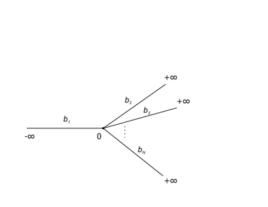
Figure 1: Star graph with $N$ semi-infinite bonds.

III Dirac equation on quantum graphs

The Dirac equation on quantum graphs has been considered first in Bulla1990 . Later, a strict treatment of the problem with the derivation of general self-adjoint vertex boundary conditions and a scattering approach was presented in Bolte .

Here, following the Ref. Bolte , we briefly recall the modelling of relativistic Dirac particles in quantum graphs. For nonrelativistic particles, the quantum graph concept has been introduced first by Exner, Seba and Stovicek Exner1 to describe free quantum motion on branched wires. In fact, the early treatment of the quantum mechanical motion in branched molecular structures dates back to the Refs. Pauling ; Rud ; Alex , who studied it in the context of organic molecules. Later, Kostrykin and Schrader Kost derived the general boundary conditions providing self-adjointness of the Schrödinger operator on graphs. Relativistic quantum mechanics described by Dirac Bolte and Bogoliubov-de Gennes operators KarimBdG on graphs have been studied recently. Parity-time (PT) symmetric quantum graphs are considered in Jambul . Hul et al. Hul considered experimental realization of quantum graphs in optical microwave networks. An important topic related to quantum graphs was studied in the context of quantum chaos theory and spectral statistics Uzy1 ; Uzy2 ; Bolte . Spectral properties and the band structure of periodic quantum graphs also attracted much interest Exner15 ; Grisha . The possibility of tuning the directed transport in quantum driven star graph has been also studied in yusupov2015 , where the reflection at the central vertex has been discussed.

Thus, quantum graphs can be determined as one- or quasi-one dimensional branched quantum wires, where the particle and wave motion can be described in terms of quantum mechanical wave equations on metric graphs by imposing the boundary conditions at the branching points (vertices) and bond ends. The metric graph itself is a set of bonds with assigned length and which are connected to each other at the vertices according to a rule called the topology of a graph, which is given in terms of the adjacency matrix Uzy1 ; Uzy2 :

$$C_{ij}=C_{ji}=\begin{cases}1&\text{ if }\;i\;\text{ and }\;j\;\text{ are connected, }\\ 0&\text{ otherwise, }\end{cases}$$

for $i,j=1,2,\dots,N$.

We start with, although the simplest, but very important, star-shaped graph shown in Fig. 1. Star graphs can be considered as the smallest building blocks for any more complicated graphs. The Dirac equation (in units $\hbar=c=1$) on each bond ($b_{j}$) of a star graph can be written as

$$\begin{split}i\partial_{t}\phi_{j}&=-i\partial_{x}\chi_{j}+m\phi_{j},\\ i\partial_{t}\chi_{j}&=-i\partial_{x}\phi_{j}-m\chi_{j}.\end{split}$$ (14)

In terms of the Dirac operator $D$ the system of equations (14) can be written as

$$i\partial_{t}\psi_{j}=D\psi_{j},$$ (15)

where $\psi_{j}=(\phi_{j},\chi_{j})^{\top}$, and

$$D:=-i\sigma_{x}\partial_{x}+m\sigma_{z},$$ (16)

with the Pauli matrices $\sigma_{x}=\begin{pmatrix}0&1\\ 1&0\end{pmatrix}$, $\sigma_{z}=\begin{pmatrix}1&0\\ 0&-1\end{pmatrix}$.

To solve Eq. (14), one needs to impose self-adjoint boundary conditions at the vertex (branching point). To do this, we introduce the following scalar product on the star graph as

$$\langle\psi,\varphi\rangle=\sum_{j=1}^{N}\int_{b_{j}}\bigl{(}\phi_{j}u_{j}^{*}+\chi_{j}v_{j}^{*}\bigr{)}\,dx,$$ (17)

where $\psi=(\psi_{1},\psi_{2},\dots,\psi_{N})$, $\varphi=(\varphi_{1},\varphi_{2},\dots,\varphi_{N})$, and $\psi_{j}=(\phi_{j},\chi_{j})^{\top}$, $\varphi_{j}=(u_{j},v_{j})^{\top}$ for $j=1,2,\dots,N$.

Defining the following skew-Hermitian scalar product on a graph

$$\begin{split}\Omega(\psi,\varphi)&=\langle D\psi,\varphi\rangle-\langle\psi,D\varphi\rangle\\ &=i\sum_{j=1}^{N}\bigl{[}\phi_{j}(0)v_{j}(0)-\phi_{j}(L_{j})v_{j}(L_{j})\\ &\quad+\chi_{j}(0)u_{j}(0)-\chi_{j}(L_{j})u_{j}(L_{j})\bigr{]}.\end{split}$$ (18)

One can prove (see, Bolte ) that self-adjointness of the Dirac operator on the graph is provided by the condition $\Omega(\psi,\varphi)=0$. A set of vertex boundary conditions fulfilling this condition can be written as

$$\begin{split}\phi_{1}(0)&=\phi_{2}(0)=\dots=\phi_{N}(0),\\ \chi_{1}(0)&+\chi_{2}(0)+\dots+\chi_{N}(0)=0,\\ \phi_{j}(L_{j})&=0,\quad j=1,2,\dots,N.\end{split}$$ (19)

The first condition represents the continuity at the vertex, while the second one provides the Kirchhoff rule at the vertex.

IV Dirac particles in transparent quantum graphs

In this section we apply the procedure presented in Section II for the derivation of transparent vertex boundary conditions for the Dirac equation on quantum graphs. It should be noted that the reflectionless motion of waves and particles in networks has been considered earlier within the different approaches in the Refs. Uzy07 ; Joly ; Naim ; Exner10 ; Kurasov ; Cheon . In Uzy07 the S-matrix based approach is utilized for the construction of scattering matrices providing the absence of backscattering. Indirect observations of the possibility for the wave transmission through the graph vertex were presented earlier in several studies, in particular by Naimark and Solomyak Naim , using some properties of the weighted Laplacian on metric graphs. The possibility for reducing a homogeneous tree graph investigation, using its symmetry, into a family of one-dimensional problems with point interactions was considered by Exner and Lipovsky Exner10 .

The existence of the reflectionless and equitransmitting vertex couplings has been studied in Kurasov ; Cheon . Despite a certain number of publications containing a study of reflectionless wave transmission through the graph vertices, all these studies did not use the concept of transparent boundary conditions for the Schrödinger equation. In Joly , the transparent boundary conditions (TBCs) are considered for the wave equation on a metric tree graph with self-similar structure at infinity, where the properties of reflectionless transport are studied numerically. However, the latter mentioned leads to very complicated numerical work, whose accuracy cannot be easily controlled. It should be noted that the direct application of TBCs for quantum graphs converts the problem into a very complicated numerical problem with almost uncontrolled accuracy.

Therefore, one needs to develop methods allowing to avoid the direct utilization of a TBC at the branching point, but instead turn the vertex boundary conditions equivalent to the TBCs. Here we combine the above concepts of TBCs and quantum graphs to design the vertex boundary conditions providing reflectionless transmission of waves through the graph branching points. In the following, such graphs will be called “transparent quantum graphs”. Recently, such an approach has been proposed for quantum graphs described by a (linear) Schrödinger equation on metric graphs tbcqg . Constraints applying the usual continuity and the Kirchhoff rule to the TBC at the vertex were found in the form of simple sum rule. An extension to the case of solitons described by the nonlinear Schrödinger equation on metric graphs has been presented in tbcnlse . Here we will use a similar approach for relativistic quasiparticles in networks modeled by the Dirac equation on quantum graphs. Such quasiparticles appear, e.g., in branched graphene nanoribbons (see, Refs. Andriotis ; Chen ; Xu ; Kvashnin ).

Let us consider a star graph shown in Fig. 1. For simplicity (without losing generality) we consider first a star graph with three bonds. To each bond $b_{j}$ of the graph we assign a coordinate $x_{j}$, which indicates the position along the bond: for bond $b_{1}$ it is $x_{1}\in(-\infty,0]$ and for $b_{1,2}$ they are $x_{2,3}\in[0,+\infty)$. In the following we use the shorthand notation $\Psi_{j}(x)$ for $\Psi_{j}(x_{j})$ and it is understood that $x$ is the coordinate on the bond $j$ to which the component $\Psi_{j}$ refers. The Dirac equation (in units $\hbar=c=1$) on each bond $b_{j}$ $(b_{1}~{}(-\infty;0],b_{2,3}~{}[0;+\infty))$ of such graph can be written as

$$\begin{split}i\partial_{t}\phi_{j}&=-i\partial_{x}\chi_{j}+m\phi_{j},\\ i\partial_{t}\chi_{j}&=-i\partial_{x}\phi_{j}-m\chi_{j}.\end{split}$$ (20)

We impose the boundary conditions at the vertex as follows

$$\alpha_{1}\phi_{1}|_{x=0} =\alpha_{2}\phi_{2}|_{x=0}=\alpha_{3}\phi_{3}|_{x=0},$$ (21)

$$\frac{1}{\alpha_{1}}\chi_{1}|_{x=0} =\frac{1}{\alpha_{2}}\chi_{2}|_{x=0}+\frac{1}{\alpha_{3}}\chi_{3}|_{x=0}.$$ (22)

We note that the vertex boundary conditions given by Eqs. (21) and (22) are self-adjoint, as they are consistent with the condition $\Omega(\psi,\varphi)=0$, where $\Omega(\psi,\varphi)$ is determined by Eq. (18).

Our task is to derive (self-adjoint) transparent vertex boundary conditions (VBCs) using the same procedure as in Section II and finding the constraints, which make the VBCs in Eqs. (21) and  (22) equivalent to the transparent ones. Such boundary conditions provide reflectionless transmission of Dirac quasiparticles at the vertex. In analogy with the procedure described in Section II, the ‘interior’ problem for the star graph is given on the bond $b_{1}$ and can be written as

$$\begin{split}i\partial_{t}\phi_{1}&=-i\partial_{x}\chi_{1}+m\phi_{1},\\ i\partial_{t}\chi_{1}&=-i\partial_{x}\phi_{1}-m\chi_{1},\\ \phi_{1}(x,0)&=\phi_{1}^{I}(x),\\ \chi_{1}(x,0)&=\chi_{1}^{I}(x),\\ (T\phi_{1})(0,t)&=\chi_{1}(0,t).\end{split}$$ (23)

The two ‘exterior’ problems on $b_{2,3}$ are given as

$$\begin{split}i\partial_{t}\phi_{2,3}&=-i\partial_{x}\chi_{2,3}+m\phi_{2,3},\\ i\partial_{t}\chi_{2,3}&=-i\partial_{x}\phi_{2,3}-m\chi_{2,3},\\ \phi_{2,3}(x,0)&=0,\\ \chi_{2,3}(x,0)&=0,\\ \phi_{2,3}(0,t)&=\Phi_{2,3}(t),\\ \chi_{2,3}(0,t)&=(T\phi_{2,3})(0,t).\end{split}$$ (24)

Further, we introduce the following Laplace transformation:

$$\widetilde{\phi}_{2,3}(x,s) =\int_{0}^{+\infty}\phi_{2,3}(x,t)\,e^{-st}\,dt,$$ (25)

$$\widetilde{\chi}_{2,3}(x,s) =\int_{0}^{+\infty}\chi_{2,3}(x,t)\,e^{-st}\,dt.$$ (26)

Then, the two ‘exterior’ problems (24) are written as

$$\begin{split}-i\partial_{x}\widetilde{\chi}_{2,3}(x,s)&=(is-m)\widetilde{\phi}_{2,3}(x,s),\\ -i\partial_{x}\widetilde{\phi}_{2,3}(x,s)&=(is+m)\widetilde{\chi}_{2,3}(x,s).\end{split}$$ (27)

The general solution of the system (27) reads

$$\begin{split}\widetilde{\phi}_{2,3}(x,s)&=c_{2,3}^{(1)}\,e^{-\sqrt[+]{s^{2}+m^{2}}x}+c_{2,3}^{(2)}\,e^{\sqrt[+]{s^{2}+m^{2}}x},\\ \widetilde{\chi}_{2,3}(x,s)&=-c_{2,3}^{(1)}\kappa\,e^{-\sqrt[+]{s^{2}+m^{2}}x}+c_{2,3}^{(2)}\kappa\,e^{\sqrt[+]{s^{2}+m^{2}}x},\end{split}$$ (28)

where $\kappa=\frac{\sqrt[+]{is-m}}{\sqrt[+]{is+m}}$. Since $\widetilde{\phi}_{2,3}$, $\widetilde{\chi}_{2,3}\in L_{2}(0;+\infty)$, we obtain for the ‘exterior’ problems on $b_{2,3}$

$$c_{2,3}^{(1)}=0,$$

hence the exterior solution is

$$\begin{split}\widetilde{\phi}_{2,3}(x,s)&=c_{2,3}^{(2)}\,e^{\sqrt[+]{s^{2}+m^{2}}x},\\ \widetilde{\chi}_{2,3}(x,s)&=c_{2,3}^{(2)}\kappa\,e^{\sqrt[+]{s^{2}+m^{2}}x}.\end{split}$$ (29)

Now, the initial conditions of the problem (24) yield

$$c_{2,3}^{(2)}=\widetilde{\phi}_{2,3}(0,s)=\widetilde{\Phi}_{2,3}(s),$$

hence

$$\begin{split}\widetilde{\phi}_{2,3}(x,s)&=\widetilde{\Phi}_{2,3}(s)\,e^{\sqrt[+]{s^{2}+m^{2}}x},\\ \widetilde{\chi}_{2,3}(x,s)&=\widetilde{\Phi}_{2,3}(s)\kappa\,e^{\sqrt[+]{s^{2}+m^{2}}x}\\ &=\kappa\widetilde{\phi}_{2,3}(x,s).\end{split}$$ (30)

From the vertex boundary conditions (21)-(22) we get

$$\begin{split}\widetilde{\phi}_{2,3}|_{x=0}&=\frac{\alpha_{1}}{\alpha_{2,3}}\widetilde{\phi}_{1}|_{x=0},\\ \widetilde{\chi}_{2,3}|_{x=0}&=\kappa\frac{\alpha_{1}}{\alpha_{2,3}}\widetilde{\phi}_{1}|_{x=0},\\ \widetilde{\chi}_{1}|_{x=0}&=\frac{\alpha_{1}}{\alpha_{2}}\widetilde{\chi}_{2}|_{x=0}+\frac{\alpha_{1}}{\alpha_{3}}\widetilde{\chi}_{3}|_{x=0}\\ &=\frac{\alpha_{1}}{\alpha_{2}}\Bigl{(}\kappa\frac{\alpha_{1}}{\alpha_{2}}\widetilde{\phi}_{1}|_{x=0}\Bigr{)}+\frac{\alpha_{1}}{\alpha_{3}}\Bigl{(}\kappa\frac{\alpha_{1}}{\alpha_{3}}\widetilde{\phi}_{1}|_{x=0}\Bigr{)}\\ &=\alpha_{1}^{2}\Bigl{(}\frac{1}{\alpha_{2}^{2}}+\frac{1}{\alpha_{3}^{2}}\Bigr{)}\kappa\widetilde{\phi}_{1}|_{x=0}.\end{split}$$ (31)

The Laplace transformed Kirchhoff rule in Eq. (22) yields

$$\chi_{1}(0,t)=A\biggl{[}\frac{d}{dt}\int_{0}^{t}I_{0}\bigl{(}m(t-\tau)\bigr{)}\phi_{1}(0,\tau)\,d\tau\\ \quad+im\int_{0}^{t}I_{0}\bigl{(}m(t-\tau)\bigr{)}\phi_{1}(0,\tau)\,d\tau\biggr{]},$$ (32)

where $A=\alpha_{1}^{2}\bigl{(}\frac{1}{\alpha_{2}^{2}}+\frac{1}{\alpha_{3}^{2}}\bigr{)}$ and $I_{0}(z)$ denotes the modified Bessel function.

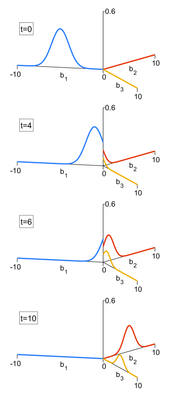
Figure 2: (color online). The position probability density $|\phi_{j}(x,t)|^{2}+|\chi_{j}(x,t)|^{2}$ plotted at different time moments for the regime when the sum rule is fulfilled (no reflection occurred): $\alpha_{1}=\sqrt{2/3}$, $\alpha_{2}=1$ and $\alpha_{3}=\sqrt{2}$.

It is clear that the boundary condition in Eq. (32) coincides with that in Eq. (12) and hence, provides reflectionless transmission of Dirac quasiparticles for the bond $b_{1}$, when $A=1$, i.e. the following sum rule is fulfilled:

$$\frac{1}{\alpha_{1}^{2}}=\frac{1}{\alpha_{2}^{2}}+\frac{1}{\alpha_{3}^{2}}.$$ (33)

The transparent boundary conditions given by Eq. (32) do not destroy the self-adjointness of the problem, since they are derived from the vertex boundary conditions (21) and (22) providing self-adjointness of the Dirac operator on the graph. We emphasize the fact that although the boundary conditions (32) are derived from those in Eqs. (21) and (22), a derivation in the opposite direction is not possible.

In this way, the vertex boundary conditions given by Eqs. (21)-(22) become equivalent to the transparent vertex boundary conditions, provided the sum rule in Eq. (33) is fulfilled.

We note that all the above results hold true for the special massless case, $m=0$, too. This is the case appearing, e.g., with the Dirac quasiparticles in graphene.

In addition, the obtained sum rule can easily be generalized for any star graph with $N$ bonds. For this general case, when the bond $b_{1}$ is considered as incoming bond, the sum rule takes form

$$\alpha_{1}^{-2}=\sum_{j=2}^{N}\alpha_{j}^{-2}$$ (34)

and the transmission of the wave (quasiparticle) in $N-1$ bonds becomes reflectionless. Furthermore, the approach can be extended for an arbitrary graph topology, having an arbitrary number of vertices, i.e. the TBC can be derived for an arbitrary metric graph. This can be easily done in an analogous way as it was shown in the Ref. tbcqg , where for example the approach was extended for a tree graph.

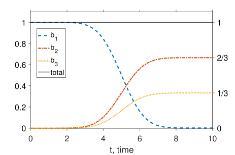
Figure 3: (color online). Time dependence of the partial and total norms for the case shown in Fig. 2.

V Numerical Experiment

This section provides the numerical justification of our obtained results. The configuration of the experimental set-up consists of a star graph with three bonds. The free time evolution of the Gaussian Dirac spinor

$$G(x)=\Bigl{(}\frac{1}{2\pi\sigma^{2}}\Bigr{)}^{1/4}\exp\Bigl{(}-\frac{(x-x_{0})^{2}}{4\sigma^{2}}\Bigr{)}\begin{pmatrix}1\\ 1\end{pmatrix}$$

compactly supported in the first bond is studied. This is done by considering the following initial conditions:

$$\begin{pmatrix}\phi_{1}(x,0)\\ \chi_{1}(x,0)\end{pmatrix}=G(x),$$

with $x_{0}=-5$, $\sigma=0.9$, and

$$\begin{pmatrix}\phi_{2,3}(x,0)\\ \chi_{2,3}(x,0)\end{pmatrix}=\begin{pmatrix}0\\ 0\end{pmatrix}.$$

We choose $m=0.01$ such that the transmission process is rather demonstrable, that is, the wave packet retains its shape for the considered time period. The leap-frog scheme (see, Hammer2014 for details) with the space discretization $\Delta x=0.0125$ and the time step $\Delta t=0.01$ is utilized for the numerical experiment. The plots in Fig. 2 show the position probability density $|\phi_{j}(x,t)|^{2}+|\chi_{j}(x,t)|^{2}$, $j=1,2,3$ at four consecutive time steps. It is clear from Fig. 2 that the wave entirely transmits to the second and third bonds without any reflections when time elapses. We note that the above boundary conditions provide the conservation of the total norm, which is defined as the sum of partial norms for each bond. The time-dependence of the partial and total norms for this case is shown in Fig. 3.

In Fig. 4 the reflection coefficient $R$ determined as the ratio of the partial norm for the first bond to the total norm

$$R=\frac{N_{1}}{N_{1}+N_{2}+N_{3}}$$

is plotted as a function of $\alpha_{1}$ for the fixed values of $\alpha_{2}$ and $\alpha_{3}$. From this plot one can conclude that the reflection coefficient becomes zero only at the value of $\alpha_{1}$ that provides the fulfillment of the sum rule (33). This observation clearly confirms once more that the sum rule in Eq. (33) turns the vertex boundary conditions in Eqs. (21)-(22) equivalent to the transparent ones.

It should also be noted here that the possibility of tuning the transition of a wave packet through the vertex comes from selecting the proper parameters $\alpha_{2}$ and $\alpha_{3}$ such that the ‘masses’ of fractions will be $N_{2}=1-\alpha_{2}^{2}/(\alpha_{2}^{2}+\alpha_{3}^{2})$ and $N_{3}=1-\alpha_{3}^{2}/(\alpha_{2}^{2}+\alpha_{3}^{2})$, accordingly.

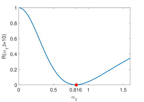
Figure 4: (color online). Dependence of the vertex reflection coefficient $R$ on the parameter $\alpha_{1}$ when the wave packet splitting time elapses ($t=10$). For fixed $\alpha_{2}=1$ and $\alpha_{3}=\sqrt{2}$, $R=0$ when $\alpha_{1}=\sqrt{2/3}\approx 0.816$ (red dot).

Let us note that Hammer, Pötz and Arnold Hammer2014 also introduced so-called discrete TBCs that were analogously derived, but for the discretized Dirac equation in 1D (using a leap-frog scheme). Finally, an “energy” functional

$$E^{n}=\rVert\phi^{n+1/2}\rVert^{2}+\rVert\chi^{n+1}\rVert^{2}\\ +\frac{\Delta t}{\Delta x}\Re\bigl{[}(D\phi^{n+1/2},\chi^{n+1})\bigr{]}=\text{const}=E^{0},$$ (35)

with the symmetric spatial difference operator

$$(D\phi^{n+1/2})_{j-1/2}=\phi^{n+1/2}_{j}-\phi^{n+1/2}_{j-1},$$

was identified, which is exactly conserved by the leap-frog scheme, even in the presence of non-constant mass and potential terms.

VI Conclusions

In this paper we studied the problem of a Dirac particle dynamics in transparent quantum graphs. These latter mentioned are determined as branched quantum wires providing reflectionless transmission of waves at the branching points. The boundary conditions for the time-dependent Dirac equation on graphs, providing absence of backscattering at the vertex are formulated explicitly. A constraint that makes the usual Kirchhoff-type boundary conditions at the vertex equivalent to those of transparent ones is derived in the form of a simple sum rule.

A reflectionless transmission of the Gaussian wave packet through the vertices, provided these constraints are fulfilled, is shown numerically for the star graph. This approach can be directly extended for arbitrary graph topologies, which contain any subgraph connected to two or more outgoing, semi-infinite bonds.

The proposed model can be applied for a broad range of practically important problems in condensed matter physics, where Dirac quasiparticles appear in branched graphene nanoribbons, CNT networks, and branched topological insulators. Moreover, the approach can be utilized for modeling polarons dynamics Campbell1981 ; Campbell1982 in branched conducting polymers, where reflectionless transmission of charge carriers through the branching points can occur.

References

- (1) A.H. Castro Neto et al., Rev. Mod. Phys. 81, 109 (2009).
- (2) V.N. Kotov, B. Uchoa, V.M. Pereira, F. Guinea, and A.H. Castro Neto, Rev. Mod. Phys. 84, 1067 (2012).
- (3) L. Brey and H.A. Fertig, Phys. Rev. B 73, 235411 (2006).
- (4) E.A. Laird, F. Kuemmeth, G.A. Steele, et. al, Rev. Mod. Phys. 87, 703, (2015).
- (5) M.Z. Hasan, C.L. Kane, Rev. Mod. Phys. 82, 3045, (2010).
- (6) X-L. Qi, S-C. Zhang, Rev. Mod. Phys. 83, 1057, (2011).
- (7) C.Chamon, R. Jackiw, Y. Nishida, S.-Y. Pi, and L. Santos, Phys. Rev. B. 81 224515 (2010).
- (8) J. Alicea, Rep. Prog. Phys. 75 076501 (2012).
- (9) T. Kottos and U. Smilansky, Ann. Phys. 76, 274 (1999).
- (10) O. Hul et al., Phys. Rev. E 69, 056205 (2004).
- (11) P. Kuchment, Waves in Random Media 14, S107 (2004).
- (12) S. Gnutzmann and U. Smilansky, Adv. Phys. 55, 527 (2006).
- (13) P. Exner and H. Kovarik, Quantum waveguides. (Springer, 2015).
- (14) B. Engquist and A. Majda, Math. Comput. 81 629, (1977).
- (15) B. Engquist and A. Majda, Commun. Pure Appl. Math. 32, 313 (1979).
- (16) L. Halpern, SIAM J. Math. Anal. 22, 1256 (1991).
- (17) I.L. Sofronov, Russian Acad. Sci. Dokl. Math. 46, 397 (1993).
- (18) A. Arnold and M. Ehrhardt, J. Comput. Phys. 145(2), 611-638 (1998).
- (19) M. Ehrhardt, VLSI Design 9(4), 325-338 (1999).
- (20) M. Ehrhardt and A. Arnold, Riv. di Math. Univ. di Parma 6(4), 57-108 (2001).
- (21) M. Ehrhardt, Acta Acustica united with Acustica 88, 711-713 (2002).
- (22) A. Arnold, M. Ehrhardt and I. Sofronov, Comm. Math. Sci. 1(3), 501-556 (2003).
- (23) S. Jiang, L. Greengard, Comput. Math. Appl. 47, 955 (2004).
- (24) X. Antoine, A. Arnold, C. Besse, M. Ehrhardt and A. Schädle, Commun. Comput. Phys. 4(4), 729-796 (2008).
- (25) M. Ehrhardt, Appl. Numer. Math. 58(5), 660-673 (2008).
- (26) L. S̆umichrast and M. Ehrhardt, J. Electr. Engineering 60(2), 301-312 (2009).
- (27) X. Antoine et al., J. Comput. Phys. 228(2), 312-335 (2009).
- (28) M. Ehrhardt, Numer. Math.: Theo. Meth. Appl. 3(3), 295-337 (2010).
- (29) P. Klein, X. Antoine, C. Besse and M. Ehrhardt, Commun. Comput. Phys. 10(5), 1280-1304 (2011).
- (30) A. Arnold, M. Ehrhardt, M. Schulte and I. Sofronov, Commun. Math. Sci. 10(3), 889-916 (2012).
- (31) R.M. Feshchenko and A.V. Popov, Phys. Rev. E 88, 053308 (2013).
- (32) X. Antoine et al., J. Comput. Phys. 277, 268-304 (2014).
- (33) P. Petrov and M. Ehrhardt, J. Comput. Phys. 313, 144-158 (2016).
- (34) T. Shibata, Phys. Rev. B 43(8), 6760 (1991).
- (35) J.-P. Kuska, Phys. Rev. B 46(8), 5000 (1992).
- (36) R. Hammer, W. Pötz, A. Arnold, J. Comput. Phys. 256, 728 (2014).
- (37) J.R. Yusupov, K.K. Sabirov, M. Ehrhardt and D.U. Matrasulov, Phys. Lett. A 383, 2382 (2019).
- (38) M.M. Aripov, K.K. Sabirov, J.R. Yusupov, Nanosystems: phys., chem., math. 10(5), 501-602 (2019).
- (39) J.R. Yusupov, K.K. Sabirov, M. Ehrhardt and D.U. Matrasulov, Phys. Rev. E 100, 032204 (2019).
- (40) W. Bulla and T. Trenkler, J. Math. Phys. 31 (5), 1157-1163 (1990).
- (41) J. Bolte and J. Harrison, J. Phys. A: Math. Gen. 36, L433 (2003).
- (42) P. Exner, P. Seba, P. Stovicek, J. Phys. A: Math. Gen. 21, 4009 (1988).
- (43) L. Pauling, J. Chem. Phys. 4 673 (1936).
- (44) K. Ruedenberg and C.W. Scherr, J. Chem. Phys. 21, 1565 (1953).
- (45) S. Alexander, Phys. Rev. B 27, 1541 (1985).
- (46) V. Kostrykin and R. Schrader J. Phys. A: Math. Gen. 32, 595 (1999).
- (47) K.K. Sabirov, J. Yusupov, D. Jumanazarov, D. Matrasulov, Phys. Lett. A, 382, 2856 (2018).
- (48) D.U. Matrasulov, K.K. Sabirov and J.R. Yusupov, J. Phys. A: Math. Gen. 52 155302 (2019).
- (49) G. Berkolaiko, P. Kuchment, Introduction to Quantum Graphs, Mathematical Surveys and Monographs AMS (2013).
- (50) J. Yusupov, M. Dolgushev, A. Blumen and O. Mülken. Quantum Inf. Process 15, 1765 (2016).
- (51) J.M. Harrison, U. Smilansky, and B. Winn, J. Phys. A: Math. Gen. 40, 14181, (2007).
- (52) P. Joly, M. Kachanovska, and A. Semin, hal-01801394, 2018.
- (53) K. Naimark and M. Solomyak, Proc. London Math. Soc. 80, 690 (2000).
- (54) P. Exner and J. Lipovsky, J. Math. Phys. 51, 122107 (2010).
- (55) P. Kurasov, R. Ogik and A. Rauf, Opuscula Math. 34, 483 (2014).
- (56) T. Cheon, Int. J. Adv. Syst. Measur. 5, 34 (2012).
- (57) A.N. Andriotis, M.Menon, Appl. Phys. Lett. 92, 042115 (2008).
- (58) Y.P. Chen, Y.E. Xie, L.Z. Sun and J. Zhong, Appl. Phys. Lett. 93, 092104 (2008).
- (59) J. G. Xu, L. Wang and M. Q. Weng, J. Appl. Phys. 114, 153701 (2013).
- (60) A.G. Kvashnin, D.G. Kvashnin, O.P. Kvashnina and L.A. Chernozatonskii, Nanotechnology 26, 385705 (2015).
- (61) D.K. Campbell and A.R. Bishop, Phys. Rev. B, 24, 8 (1981).
- (62) D.K. Campbell and A.R. Bishop, Nuclear Physics B, 200 [FS4], 297-328 (1982).