COVID-19: $R_{0}$ is lower
where outbreak is larger

Abstract

We use daily data from Lombardy, the Italian region most affected by the COVID-19 outbreak, to calibrate a SIR model individually on each municipality. These are all covered by the same health system and, in the post-lockdown phase we focus on, all subject to the same social distancing regulations. We find that municipalities with a higher number of cases at the beginning of the period analyzed have a lower rate of diffusion, which cannot be imputed to herd immunity. In particular, there is a robust and strongly significant negative correlation between the estimated basic reproduction number ($R_{0}$) and the initial outbreak size, in contrast with the role of $R_{0}$ as a predictor of outbreak size. We explore different possible explanations for this phenomenon and conclude that a higher number of cases causes changes of behavior, such as a more strict adoption of social distancing measures among the population, that reduce the spread. This result calls for a transparent, real-time distribution of detailed epidemiological data, as such data affects the behavior of populations in areas affected by the outbreak.

Keywords: COVID-19, tests, basic reproduction number, social distancing, containment.
JEL classification: I12, I18, C53, C22.

1 Introduction

The basic reproduction number, or $R_{0}$, represents the average number of secondary cases produced by a single infected case in an otherwise susceptible population, and it is typically used as a reference value to assess the transmissibility of an infectious disease in a given population. Given a number of individuals susceptible to infection, a disease with higher $R_{0}$ will infect a larger number of individuals. There is hence an obvious positive relationship between the $R_{0}$ and the resulting size of an outbreak (Tildesley and Keeling, 2009).

However, the value of $R_{0}$ during an outbreak does not only depend on ex-ante features of a virus or a population, but potentially also on the response of both population and authorities to the outbreak. This is particularly true in the context of the COVID-19 pandemic, to which most countries in the world have reacted with some form of social distancing measures, or lockdown. In absence of a vaccine or effective drugs, these measures are the best weapon to reduce the number of deaths, as well as the number of intensive care unit beds required (Kucharski et al., 2020; Flaxman et al., 2020; Ferguson et al., 2020; Greenstone and Nigam, 2020).

In the present study, we analyze data on the diffusion of COVID-19 in Lombardy, the region of Italy most heavily affected by the pandemic (Cereda et al., 2020 provide an accurate description of the early phase of the outbreak in such region). Specifically, we employ daily data on the number of individuals positive to COVID-19 at the municipality level, focusing on a period in which the entire country was subject to a lockdown. All municipalities under analysis share the same public health system and, in the period considered, were subject to the same social distancing regulation. However, at the start of the period, they were characterized by a strong heterogeneity in the number of cases, both in absolute terms and in terms of cases per capita.

We study a period beginning on March 25, 2020, that is, more than two weeks after the lockdown regulation was put in place, and ending with April 14, when such regulations still held: this means that movements across municipalities are severely restricted, requiring any travelers to present a valid (typically work or health related) justification for their journey.

We fit a Susceptible-Infected-Recovered (SIR) model on data from each municipality and find that the estimated $R_{0}$ is negatively correlated with the prevalence in the municipality at the beginning of our period. This result holds both when considering the absolute and per capita number of cases and is robust to different specifications and sample disaggregations.

We present and compare different complementary explanations for this finding. Early and widespread testing increases the reported number of cases and might allow the authorities to slow the spread of the pandemic by isolating known cases. At the same time, where the number of cases is higher, the population might comply more strictly with the lockdown measures, thus reducing the rate of spread: we show in Section 4.1 why the latter mechanism is most likely to drive our results.

2 Data

We employ count data of per-municipality recorded cases, updated daily and distributed by regional authorities. We do not rely on data on recovered and deceased individuals, as such data are not available with the required geographical disaggregation.

Data are available starting from March 25, 2020 and cover a period of twenty-one days during which lockdown measures were always in place. We verify that only minimal deviations appear between regional data and the aggregation of municipal data. Out of 1507 municipalities in Lombardy, 960 had at least one recorded COVID-19 case as of this date. Figure 1(a) displays the number of cases (size of the dots) and the cases per capita (color of the dots) as of March 25 for each of these 960 municipalities. Similarly, Figure 1(b) displays the number of new cases (size of the dots) and the number of new cases per capita (color of the dots) recorded in each municipality between March 25 and April 14.

Figure 1: Distribution of cases and cases increase

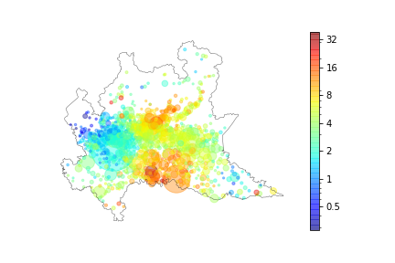
(a) Cases on March 25

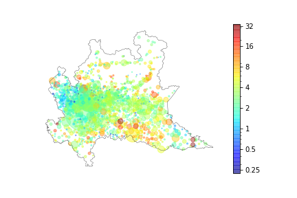
(b) New cases between March 25 and April 14

Note: dot size represent absolute numbers, colors represent cases per one thousand inhabitants.

It should be noted that official data concerning the COVID-19 outbreak in Italy has been found to be strongly incomplete, both in terms of positive individuals and of casualties: several researchers have estimated an outbreak size much higher than that suggested by official numbers (Flaxman et al., 2020), while others have corroborated this with an analysis of anomalies in death rates. Moreover, local testing strategies are known to have deviated from WHO guidelines and have changed over time, also depending on available resources: towards the end of our period of interest, more subjects with mild symptoms were tested. For this reason, some researchers have put forwards adaptations of the SIR model that account for a threshold in the capacity of the health system. Such problems are not specific to Italy, as official data from a number of countries have been questioned. More in general, the difficulty in obtaining reliable data on the number of infected, deceased and recovered individuals calls for refinements of traditional epidemiologic models (Atkeson et al., 2020; Riccardo et al., 2020).

Given our research question, these caveats are of limited importance. Indeed, the focus of the present work is to document differences in response across municipalities, rather than to precisely estimate the epidemiological parameters or expected duration of the COVID-19 outbreak in Lombardy.

Data on population size is obtained from the Italian National Istitute of Statistics (ISTAT).

3 Methods

We fit a SIR model on each municipality in the period of twenty-one days beginning in March 25. Given the short time span considered, we employ a simplified SIR model which does not account for natural rate of mortality. Hence, the model is entirely defined by setting few parameters: $\beta$, which determines the rate at which susceptible ($S$) individuals become infected ($I$); $\gamma$, which determine the rate at which infected individuals become recovered ($R$); the initial number of infected and recovered individuals, and the population size $N$ ($=S+I+R$). We take population size from official statistics. We hence consider a discretized version of the continuous SIR model – each period corresponding to a day – and automatically explore the parameter space for $\beta$, $\gamma$, and the initial value for $I$ and $R$, looking for the combination that provides the best fit. Specifically, the goodness of fit is maximized by minimizing the sum of square residuals between the cases count and the sum of the $I$ and $R$ pools sizes. The initial values for the free parameters are set to those calibrated on the entire Lombardy region.

Given that the SIR model assumes a non-null initial population of infected individuals, we only consider the 960 municipalities satisfying this condition. We further drop 47 municipalities which had new cases recorded on only one or two dates, hence reducing to 913 municipalities. Although this sample selection might in principle affect our results, we show in Section 4.2 that this is not the case.

Figure 2(a) displays the fit between data at the regional level and the corresponding simulated SIR model. Figures 2(b) and 2(c) are the equivalent for Milan and Castiglione d’Adda: these are the two municipalities which, at the beginning of our period of interest, had been most heavily hit in absolute and per capita terms, respectively. Note that a weekly fluctuation can be observed for all municipalities: this is in line with documented evidence that less tests are processed during the weeekend, and the effect reverberates on the number of positive detected cases with a delay of two to three days. We expect these fluctuations to affect the entire region homogeneously.

Figure 2: Comparison of fitted SIR model and total cases count

(a) Lombardy

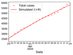
(b) Milan

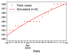
(c) Castiglione d’Adda

Note: fit between data and the corresponding SIR model for Lombardy region (left) and the most affected municipalities at the beginning of our period of interest in absolute and per capita terms, respectively (center, right).

Once we find the best SIR parameters for each municipality, we regress the estimated $R_{0}$ (the ratio of the estimated $\beta$ and $\gamma$) on the outbreak size within the municipality as of March 25. We focus on the per capita number of cases, as we expect any effect to be related to the prevalence of the outbreak – a same number of cases will be perceived in a very different way in Milan or in a small municipality.

4 Results

Figure 3: Distribution of $R_{0}$

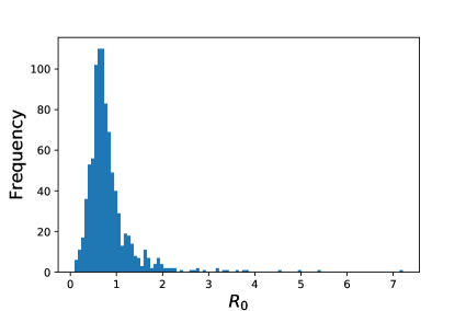
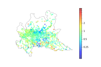
Note: distribution of estimated per-municipality $R_{0}$, computed as $\frac{\beta}{\gamma}$.

Figure 3 shows the distribution of the estimated values of $R_{0}$: the mean estimated value is 0.83 (0.85 when weighted on population), while the median is 0.70A strong heterogeneity (which can be partly attributed to statistical noise – several municipalities count only a few cases each) can be observed across municipalities: in what follows, unless differently specified, we trim data by dropping 0.5% of outliers on each side of the distribution of $R_{0}$, hence reducing to 903 municipalities. In only few of these (179) the value of $R_{0}$ appears to be larger than the critical threshold of 1: that is, in the vast majority of municipalities, the outbreak is expected to spontaneously extinguish without requiring herd immunity.

Table 1: Main results

	(1)	(2)	(3)	(4)
Intercept	0.920∗∗∗	0.921∗∗∗	0.906∗∗∗	0.823∗∗∗
	(0.024)	(0.025)	(0.025)	(0.016)
cases‰	-0.023∗∗∗	-0.023∗∗∗	-0.032∗∗∗
	(0.004)	(0.004)	(0.005)
cases			-0.000	-0.001∗∗∗
			(0.000)	(0.000)
population		-0.000		0.000∗∗∗
		(0.000)		(0.000)
population-1			180.274∗∗∗
			(57.829)
Observations	903	903	903	903
R${2}$	0.036	0.036	0.048	0.015

Note: dependent variable $R_{0}$. ^∗p$<$0.1; ^∗∗p$<$0.05; ^∗∗∗p$<$0.01

Table 1 presents the results of the regression analysis. We see a negative and strongly significant relationship between the initial number of cases per one thousand inhabitants and the estimated $R_{0}$ (column (1)); this relationship is robust to controlling for population size (column (2)), and to both the absolute number of cases and the inverse of population size (column (3)), i.e., a full interaction model where the the per capita count represents the interaction term (Kronmal, 1993). The coefficient for the per capita number of cases can be interpreted as the reduction in $R_{0}$ resulting from an increase of one case per one thousand individuals in the prevalence of the outbreak. The value of -0.023 observed in column (2), which we consider as our baseline specification, indicates a sizeable effect: for reference, given that the prevalence in Milan as of March 25 was of around $1.7$‰, the above mentioned result suggests that had it been $2.7$‰, the average $R_{0}$ would have been around 0.88 instead than the observed 0.90. The same negative and strongly significant effect is observed if we focus on the absolute number of cases as explanatory variable, controlling for the population size (column (4)).

It should be noted that any intrinsic characteristic of municipalities – such as demography, location, structure of the economy – which might explain a larger outbreak size should also favor a larger $R_{0}$ (Mills, 2020). Thus, controlling for such characteristics is expected to further reduce the coefficient for cases‰.

4.1 Interpretation

There are a few reasons that might explain why a larger outbreak should result in a subsequent lower $R_{0}$.

The first might be related to herd immunity, by which areas where the outbreak is initially more present have less scope for further spread because a large share of individuals have already caught, and possibly developed immunity to, the virus. This is in principle not a problem of our approach, as the SIR model accounts for this effect and should estimate an $R_{0}$ net of it – in other terms, $R_{0}$ describes the evolution of the outbreak in an hypothetical situation in which the pool of susceptible individuals is never reduced. However, the problem might still arise if the count data employed severely underestimate the actual spread of the virus: the number of positive cases could actually be much larger than the detected one, leading to an estimated $R_{0}$ lower than the real one because of the undetected effect of herd immunity in reducing the rate of contagion.

The underestimation of infected population might also suggest an alternative explanation of the result related to test capacity: to the extent that a lower detected prevalence reflects a lower ability of authorities to identify infected individuals, it should then correlate with a lower ability to isolate, hospitalize and cure them, and hence to a faster outbreak growth.

A third, social, explanation is instead that wherever the local population is aware of a larger prevalence of the disease, it reacts by changing its behavior towards a stricter application of social distancing rules, thus leading to a lower $R_{0}$. In what follows, we provide evidence in favor of this hypothesis.

We start by analyzing the first possible explanation: several sources have argued that the actual size of the infected population might lie between four and ten times the official reported numbers. In the most affected muncipalities in our sample during the period analyzed, 57 infections per one thousand inhabitants have been recorded, and according to the most pessimistic estimates this would mean that up to $57\%$ of the population was infected. While most municipalities have a number of recorded cases per one thousand inhabitants which is orders of magnitude lower, to avoid the possibility that an even partial herd immunity effect might be driving the results, we re-estimate our main model on subsamples of municipalities according to their initial number of cases per capita. Specifically, we split the sample according to quartiles of cases per capita on March 25. The results, presented in columns (1) to (4) of Table 2, show that our findings are not driven by herd immunity, as the coefficient for cases‰ is negative in each quartile. The absolute value of such coefficient is actually much larger for municipalities with a low prevalence than for those with a higher prevalence, and is strongly significant in the first two quartiles, hence including municipalities with 2 cases per one thousand inhabitants or less.

We then consider the second possible explanation: that a lower detected prevalence signals a lower detection ability, and that this naturally correlates with lower ability to track and quarantine infected subjects, hence raising the subsequent rate of diffusion. In order to disentangle this test capacity explanation from the third, social, one, we sketch two simple models of how these would be expected to affect $R_{0}$.

Let us represent with $u_{t}$ the unknown real number of infected subjects per one thousand inhabitants, at time $t$ in a given municipality, and with $i_{t}$ the corresponding known number. We are interested in the extent to which unidentified infected subjects (which are $u_{t}-i_{t}$ cases per one thousand inhabitants) will raise the $R_{0}$ for the municipality in the subsequent period. More specifically, we can assume that identified and unidentified patients form two different pools of infected subjects and that the latter has a much higher $\beta$ – probability of infecting susceptible individuals – that leads to a corresponding higher $R_{0}$. Since $\beta$ enters linearly in $R_{0}$ – and assuming for simplicity that $\gamma$ is constant – the relationship between $u_{t}-i_{t}$ and $R_{0}$ would be expected to be linear. Moreover, it is well known that not only identified patients are subject to a stronger form of isolation, but also close contacts of such patient (some of which are not infected) are recommended to self-quarantine: this does not happen in municipalities with a larger number of undetected cases, which implies that the effect of each unidentified patient should be more than linear in increasing the $R_{0}$. This would imply a linear or concave relationship between cases‰ and $R_{0}$.

Vice-versa, any social explanation is based on the assumption that inhabitants react to the news of the cases in their municipality. Given any concave function describing this reaction, a same increase in per capita cases will be perceived as more important if the initial number of cases is lower. That is, we can expect inhabitants of two towns with respectively 1 and 11 known cases per one thousand inhabitants to differ in their compliance with social distancing prescriptions more than inhabitants of two towns with respectively 20 and 30 known cases per one thousands inhabitants: a same difference of one percentage point in prevalence will have a weaker effect on people behavior were prevalence is higher. This alternative explanation predicts a convex relationship (given the negative sign) between $cases$‰ and $R_{0}$.

Table 2: Additional specifications

	Q 1	Q 2	Q 3	Q 4	Full
	(1)	(2)	(3)	(4)	(5)
Intercept	1.071∗∗∗	1.290∗∗∗	0.899∗∗∗	0.760∗∗∗	0.992∗∗∗
	(0.066)	(0.185)	(0.206)	(0.098)	(0.033)
cases‰	-0.098∗∗	-0.125∗∗	-0.033	-0.004	-0.050∗∗∗
	(0.045)	(0.057)	(0.039)	(0.009)	(0.009)
cases‰2					0.002∗∗∗
					(0.001)
population	0.000	-0.000	0.000	-0.000	-0.000
	(0.000)	(0.000)	(0.000)	(0.000)	(0.000)
Observations	226	226	225	226	903
R${2}$	0.021	0.027	0.005	0.008	0.047

Note: dependent variable: estimated $R_{0}$. Columns (1) to (4): model restricted to municipalities with a number of cases per thousand inhabitants in the interval (0.278, 2.177], (2.177, 4.124], (4.124, 6.277] and (6.277, 30.973], respectively. Column (5): full sample. ^∗p$<$0.1; ^∗∗p$<$0.05; ^∗∗∗p$<$0.01

To disentangle between the test capacity and the social explanation, we enrich our basic model by introducing a quadratic term in cases‰. This is done in column (5) of Table 2. We see that the quadratic term has a positive sign and is strongly significant, while the sign of the linear term is still negative and has increased in absolute terms. Hence, while this does not allow us to exlude that the other explanations might play a role, we can conclude that the social explanation is the main driver of the negative relationship between cases‰ and $R_{0}$.

(Jones et al., 2020) describes two possible opposite reactions to the COVID-19 oubreak: a precautionary attitude that leads to a stricter adherence to guidelines, and a “fatalism effect” according to which an individual who is more likely to be infected in the future “reduces her incentives to be careful today”. Our results provide strong evidence in favor of the first mechanism.

4.2 Sensitivity tests

In addition to the quantile analysis previously described, we verify that our main result also holds consistently across the 12 provinces (lower level administrative regions) of which Lombardy is composed. Results are displayed in Figure 4(a). We see that, for each province, the effect of cases‰ on $R_{0}$ is negative: although the small sample size results in only few provinces reaching statistical significance, it is clear that no specific area of Lombardy is alone responsible for our findings.

Figure 4:

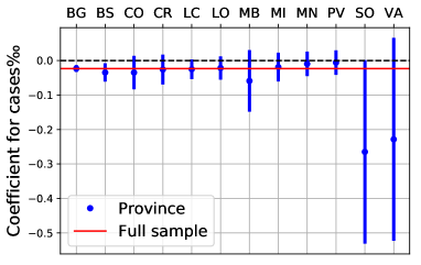
(a) Disaggregated estimation across provinces

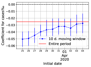
(b) Estimation over 10-days moving windows

Note: estimates are run controlling for population, as in column (2) of Table 1; the red line denotes the corresponding coefficient estimated on the entire sample under analysis.

In order to verify that our results do not strictly depend upon the period considered, we replicate our analysis over different 10-days moving windows within our period of analysis. For each subperiod, we fit the $R_{0}$ for each municipality and regress it on the number of cases per thousand individuals at the beginning of that subperiod. In accordance with the selection procedure described in Section 3, we reduce this analysis to the 713 municipalities that feature at least one case on March 25 and, in each window, have new cases recorded in at least two dates. The results are shown in Figure 4(b). For comparability, we also display the value of the coefficient estimated for the entire time period on the same restricted sample of 713 municipalities. We find that the effect of interest is robust, that is, the coefficient for the cases‰ is consistently negative and strongly significant for each subperiod. Its absolute value is significantly decreasing over time; that is, the effect of the number of cases on the $R_{0}$ in the following days appears to be stronger in the earlier days of the outbreak. While there might be multiple explanations for this, we only remark that the rate of growth of the epidemic has been consistently decreasing: whether individual behavior reacts not just to outbreak size, but also to its change over time, is an issue for further research.

Finally, we verify that all results reported in Table 1, including statistical significance, are virtually unchanged if we do not trim the data as previously described.

4.3 Prediction of outbreak duration

While an accurate predition of the date of extinction of the outbreak deserves more sophisticated epidemiologic models (Guzzetta et al., 2020; Riccardo et al., 2020) that are out of the scope of the present paper, we can analyze to some extent the relationship between the predicted date of extinction and the number of initial cases.

In general, the relationship between infected population at time $t$ and expected date of extinction of the outbreak within a SIR model depends on the size of $R_{0}$: if the latter is smaller than 1 – i.e., the outbreak is spontaneously slowing – then a smaller outbreak will extinguish sooner; vice-versa, if $R_{0}>1$, a larger outbreak will sooner reach a level of herd immunity, and hence die out.

Since, according to our data, most municipalities in Lombardy display an $R_{0}<1$, we focus on this case. While for a same level of $R_{0}$ we expect the predicted time to extinction to increase with the initial outbreak size, the fact that the $R_{0}$ is negatively related to initial outbreak size – and that a lower $R_{0}$ leads to a quicker extinction – leaves theoretically undetermined the relationship between initial outbreak size and duration of the outbreak.

Table 3: Outbreak size and expected outbreak duration

	Full	$R_{0}$<1	Full	$R_{0}$<1
	(1)	(2)	(3)	(4)
Intercept	214.957∗∗∗	56.873∗∗∗	317.477∗∗∗	142.455∗∗∗
	(24.500)	(13.010)	(17.771)	(11.028)
cases‰	7.032∗	8.198∗∗∗
	(3.999)	(2.082)
cases			-0.339	0.114
			(0.353)	(0.201)
population	-0.000	0.000	0.001	0.000
	(0.000)	(0.000)	(0.001)	(0.000)
Observations	903	729	903	729
R${2}$	0.004	0.021	0.002	0.005

Note: dependent variable: days to expected outbreak extinction. “Extinction” is defined as reaching 0.1 cases per one thousand inhabitant in columns (1) and (2), 0.1 cases in columns (3) and (4). ^∗p$<$0.1; ^∗∗p$<$0.05; ^∗∗∗p$<$0.01

In order to shed light on this indeterminacy, we proceed to simulating the SIR model for each municipality until the predicted size of the infected population decreases below either (i) 0.1 cases for one thousands inhabitants or (ii) 0.1 cases and we consider the number of periods elapsed as the outbreak duration. We then regress the outbreak duration, defined in these two different ways, over the initial (i) number of cases per capita (columns (1) and (2) of Table 3) and (ii) absolute number of cases (columns (3) and (4) of Table 3), respectively.

Results from Table 3 show that the relationship between outbreak size and extinction date is non-trivial. First, the relatively few municipalities with $R_{0}>1$ do influence significantly the results – as already discussed, the expected effect of outbreak size for a same $R_{0}$ is reversed in such cases. Second, if we restrict to $R_{0}<1$, the relationship is positive and significant when reasoning in per capita terms, but not in absolute terms. It should also be mentioned that the results depend on the thresholds adopted in the definition of outbreak extinction. In general, given that $R_{0}<1$ determines the exponential decay, a lower threshold will mean that the date of extinction is further away for municipalities with a relatively low number of cases and relatively high $R_{0}$.

Summing up, the results of predicting the extinction date are to be interpreted as cautionary: municipalities with smaller outbreaks might get rid of them sooner than others with more infected individuals (column (2) of Table 3), but this result does not generalize to the absolute outbreak size (columns (3) and (4) – the former even featuring a negative sign). Plans for a gradual exit from lockdown should take into account that the relationship between outbreak size and expected outbreak duration is difficult to pinpoint – as well as the possibility that a larger outbreak might bring the population closer to herd immunity, making it more resistent to a new outbreak.

5 Conclusion

We show that in Lombardy, during a lockdown, the basic reproduction number for COVID-19 reacts negatively to the initial size of an outbreak at the municipality level, an effect which cannot be explained by the population having reached herd immunity. Limited test capacity – and hence a limited ability by health authorities to isolate and treat affected individuals – appear to have at most a marginal role in explaining our result. Instead, we show that the population’s behavior is key to slowing down the contagion and in particular that information about local outbreaks impacts on diffusion rates. This effect is consistent across all provinces and it is robust to the sample period considered.

The fact that the effect is particularly strong in municipalities characterized by a smaller outbreak suggests that individuals react more strongly to the first few cases. This aspect is confirmed by the convex relationship we find between the initial size of the outbreak and the $R_{0}$: the marginal effect on behavior of each new case seems to decrease in the number of cases.

Our results provide evidence in favor of a precautionary rather than fatalistic individual attitude towards the outbreak. They call for considering the population as an integral part of the decision making process, and for a timely and transparent provision of epidemiologic data.

Supplementary information

Optimization procedure

For simplicity, the procedure for fitting the SIR model is implemented over the parameters $R_{0}$ and $\gamma$ rather than $\beta$ and $\gamma$, where $R_{0}=\frac{\beta}{\gamma}$. For each parameter (including the initial values $I=\hat{I}$ and $R=\hat{R}$), the procedure is initialized by deriving reasonable values based on tuning the model to regional aggregated data.

Then the procedure works as follows ($i$ denotes an iteration, $\delta_{\pi,1}$ is set to $0.2$ for each parameter $\pi$):

1. given the current value of a parameter $\pi_{i}$, compute values of the parameter $\pi_{i-l}=\pi_{i}\times(1-\delta_{\pi,i})$ and $\pi_{i,r}=\pi_{i}\times(1+\delta_{\pi,i})$ (the right and left candidate values for parameter $\pi$),

2. compare count data and the simulation obtained with each of the three candidates $\pi_{i,l}$, $\pi_{i}$ and $\pi_{i,r}$ by computing the sum of squared residuals,

3. select the candidate value which results in the smallest error as new parameter value $\pi_{i+1}$,

4. if the value did not change (that is, $\pi_{i+1}=\pi_{i}$), set $\delta_{\pi,i+1}=\delta_{\pi,i}\cdot 0.75$; otherwise, leave $\delta_{\pi,i+1}=\delta_{\pi,i}$,

5. repeat steps from 1 to 4 for each parameter $\pi\in\{R_{0},\gamma,\hat{I},\hat{R}\}$,

6. repeat steps from 1 to 5 until $\delta_{\pi,i}<0.001$ for each parameter.

References

- Atkeson et al. (2020) Atkeson, A. et al. (2020). How deadly is covid-19? understanding the difficulties with estimation of its fatality rate. Technical report, Federal Reserve Bank of Minneapolis.
- Cereda et al. (2020) Cereda, D., M. Tirani, F. Rovida, V. Demicheli, M. Ajelli, P. Poletti, F. Trentini, G. Guzzetta, V. Marziano, A. Barone, M. Magoni, S. Deandrea, G. Diurno, M. Lombardo, M. Faccini, A. Pan, R. Bruno, E. Pariani, G. Grasselli, A. Piatti, M. Gramegna, F. Baldanti, A. Melegaro, and S. Merler (2020). The early phase of the covid-19 outbreak in lombardy, italy.
- Ferguson et al. (2020) Ferguson, N., D. Laydon, G. Nedjati-Gilani, N. Imai, K. Ainslie, M. Baguelin, S. Bhatia, A. Boonyasiri, Z. Cucunubá, G. Cuomo-Dannenburg, et al. (2020). Impact of non-pharmaceutical interventions (npis) to reduce covid-19 mortality and healthcare demand. imperial college covid-19 response team.
- Flaxman et al. (2020) Flaxman, S., S. Mishra, A. Gandy, et al. (2020). Estimating the number of infections and the impact of nonpharmaceutical interventions on covid-19 in 11 european countries. Imperial College COVID-19 Response Team 30.
- Greenstone and Nigam (2020) Greenstone, M. and V. Nigam (2020). Does social distancing matter? University of Chicago, Becker Friedman Institute for Economics Working Paper (2020-26).
- Guzzetta et al. (2020) Guzzetta, G., P. Poletti, M. Ajelli, F. Trentini, V. Marziano, D. Cereda, M. Tirani, G. Diurno, A. Bodina, A. Barone, L. Crottogini, M. Gramegna, A. Melegaro, and S. Merler (2020). Potential short-term outcome of an uncontrolled covid-19 epidemic in lombardy, italy, february to march 2020. Eurosurveillance 25(12), 2000293.
- Jones et al. (2020) Jones, C., T. Philippon, and V. Venkateswaran (2020). Optimal mitigation policies in a pandemic: Social distancing and working from home.
- Kronmal (1993) Kronmal, R. A. (1993). Spurious correlation and the fallacy of the ratio standard revisited. Journal of the Royal Statistical Society: Series A (Statistics in Society) 156(3), 379–392.
- Kucharski et al. (2020) Kucharski, A. J., T. W. Russell, C. Diamond, Y. Liu, J. Edmunds, S. Funk, R. M. Eggo, F. Sun, M. Jit, J. D. Munday, et al. (2020). Early dynamics of transmission and control of covid-19: a mathematical modelling study. The Lancet Infectious Diseases.
- Mills (2020) Mills, M. (2020, Mar). Demographic science covid-19.
- Riccardo et al. (2020) Riccardo, F., M. Ajelli, X. Andrianou, A. Bella, M. Del Manso, M. Fabiani, S. Bellino, S. Boros, A. Mateo Urdiales, V. Marziano, M. C. Rota, A. Filia, F. P. D’Ancona, A. Siddu, O. Punzo, F. Trentini, G. Guzzetta, P. Poletti, P. Stefanelli, M. R. Castrucci, A. Ciervo, C. Di Benedetto, M. Tallon, A. Piccioli, S. Brusaferro, G. Rezza, S. Merler, and P. Pezzotti (2020). Epidemiological characteristics of covid-19 cases in italy and estimates of the reproductive numbers one month into the epidemic. medRxiv.
- Tildesley and Keeling (2009) Tildesley, M. J. and M. J. Keeling (2009). Is R0 a good predictor of final epidemic size: Foot-and-mouth disease in the UK. Journal of theoretical biology 258(4), 623–629.