Non-orientable branched coverings, $b$-Hurwitz numbers, and positivity for multiparametric Jack expansions

Abstract.

We introduce a one-parameter deformation of the 2-Toda tau-function of (weighted) Hurwitz numbers, obtained by deforming Schur functions into Jack symmetric functions. We show that its coefficients are polynomials in the deformation parameter $b$ with nonnegative integer coefficients. These coefficients count generalized branched coverings of the sphere by an arbitrary surface, orientable or not, with an appropriate $b$-weighting that “measures” in some sense their non-orientability.

Notable special cases include non-orientable dessins d’enfants for which we prove the most general result so far towards the Matching-Jack conjecture and the “$b$-conjecture” of Goulden and Jackson from 1996, expansions of the $\beta$-ensemble matrix model, deformations of the HCIZ integral, and $b$-Hurwitz numbers that we introduce here and that are $b$-deformations of classical (single or double) Hurwitz numbers obtained for $b=0$.

A key role in our proof is played by a combinatorial model of non-orientable constellations equipped with a suitable $b$-weighting, whose partition function satisfies an infinite set of PDEs. These PDEs have two definitions, one given by Lax equations, the other one following an explicit combinatorial decomposition.

1. Introduction

Hurwitz numbers and tau-functions. Hurwitz numbers, in their most general sense, count the number of combinatorially inequivalent branched coverings of the sphere by an orientable surface with a given number of ramification points and given ramification profiles. Hurwitz numbers and their variants (dessins d’enfants, weighted, monotone, orbifold Hurwitz numbers) have numerous connections to mathematical physics, combinatorics, and the moduli spaces of curves [Kon92, GJ97, ELSV01, GV03, GJV05, OP06, Mir07, GPH17].

Hurwitz himself [Hur91] showed that Hurwitz numbers can be expressed in terms of characters of the symmetric group. Equivalently, generating functions of Hurwitz numbers can be expressed explicitly in terms of Schur functions, which gives them a rich structure. A fundamental fact in the field, whose origins go back to Pandariphande [Pan00], Okounkov [Oko00], Orlov and Scherbin [OS00], and now understood in a wide generality (see e.g. [GJ08, GPH17]) is that Hurwitz numbers can be used to define a formal power series which is a tau-function of the KP, or more generally 2-Toda hierarchy [MJD00]. Explicitly, in the case of $k+2$ ramification points, this tau-function has the form

(1) $$\tau^{(k)}(t;\mathbf{p},\mathbf{q},u_{1},\dots,u_{k}):=\sum_{n\geq 0}t^{n}\sum_{\lambda\vdash n}\left(\frac{f_{\lambda}}{n!}\right)^{2}\tilde{s}_{\lambda}(\mathbf{p})\tilde{s}_{\lambda}(\mathbf{q})\tilde{s}_{\lambda}(\underline{u_{1}})\tilde{s}_{\lambda}(\underline{u_{2}})\dots\tilde{s}_{\lambda}(\underline{u_{k}}),$$

where $\tilde{s}_{\lambda}=\frac{n!}{f_{\lambda}}\cdot s_{\lambda}$ is the normalized Schur function indexed by the integer partition $\lambda$ of $n$, expressed as a polynomial in the power-sum variables $\mathbf{p}=(p_{i})_{i\geq 1}$ or $\mathbf{q}=(q_{i})_{i\geq 1}$, where $\underline{u}=(u,u,\dots),$ and where $f_{\lambda}$ is the dimension of the irreducible representation of the symmetric group indexed by $\lambda$. From this function (or more precisely its logarithm) one can extract all the forms $\omega_{g,n}$ associated to the contribution of coverings from surfaces of genus $g$ with $n$ boundaries, which obey the Chekhov-Eynard-Orantin topological recursion [CEO06, EO07, ACEH20]. Weighted Hurwitz numbers [GPH17] correspond in some sense to the case $k=\infty$, which contains the Okounkov-Pandariphande Hurwitz numbers as a special case (see Section 6). The case $k=1$ (three ramification points) corresponds to dessins d’enfants or Belyi curves (bipartite maps in the language of combinatorialists).

Jack polynomials and $b$-deformations. In this paper we consider the one-parameter deformation, or $b$-deformation, of the function $\tau^{(k)}$ defined by

(2) $$\tau^{(k)}_{b}(t;\mathbf{p},\mathbf{q},u_{1},\dots,u_{k}): =\sum_{n\geq 0}t^{n}\sum_{\lambda\vdash n}\frac{1}{j_{\lambda}^{(\alpha)}}J_{\lambda}^{(\alpha)}(\mathbf{p})J_{\lambda}^{(\alpha)}(\mathbf{q})J_{\lambda}^{(\alpha)}(\underline{u_{1}})\dots J_{\lambda}^{(\alpha)}(\underline{u_{k}}),$$

where $J^{(\alpha)}_{\lambda}$ is the Jack symmetric function of parameter $\alpha=1+b$, for formal or complex $b$, and where $j_{\lambda}^{(\alpha)}$ is a natural $b$-deformation of $n!^{2}/{f_{\lambda}^{2}}$, see Section 5.

Jack functions are obtained as a one-parameter limit of Macdonald polynomials that interpolates between Schur and zonal polynomials, respectively for $b=0,1$ [Jac71, Mac95]. In particular the function $\tau^{(k)}_{b}$ is equal to $\tau^{(k)}$ for $b=0$. Many classical problems in algebraic combinatorics (dealing with symmetric functions, maps, coverings, tableaux, partitions) are connected to Schur or zonal polynomials. Understanding how to use Jack symmetric functions to build continuous deformations between them has become an important research goal in the last decades, see [Sta89, HSS92, GJ96, DF16, BGG17, GH19]. It often requires to develop new methods that shed new light even on the most classical results. In our context, the deformation (2) was introduced by Goulden and Jackson [GJ96] in the case $k=1$ of dessins d’enfants and is strongly related to the Matching-Jack conjecture and the $b$-conjecture of these authors, see the discussion below.

Non-orientable branched coverings. Our main result gives a geometric (and combinatorial) meaning to the coefficients of $\tau^{(k)}_{b}$ in terms of generalized branched coverings of the sphere. Let $\mathcal{S}$ be a compact connected surface, orientable or not, and let $\mathbb{S}^{2}$ denote the two-dimensional sphere. Let $\widetilde{\mathcal{S}}$ be the orientation-double-cover of $\mathcal{S}$. A generalized branched covering of $\mathbb{S}^{2}$ by $\mathcal{S}$ is a continuous function $f:\mathcal{S}\rightarrow\mathbb{S}^{2}_{+}$ from $\mathcal{S}$ to the closed upper hemisphere $\mathbb{S}^{2}_{+}$, which can be lifted to a branched covering $\tilde{f}:\widetilde{\mathcal{S}}\rightarrow\mathbb{S}^{2}$ in a certain sense. A precise definition, together with the definition of degree, ramification points and ramification profiles, is given in Section 2.

Generalized branched coverings with $k+2$ ramification points are in bijection (Section 2) with some combinatorial embedded graphs on the surface $\mathcal{S}$ that we call $k$-constellations. These objects come with a natural notion of rooting which consists in marking and orienting an angular sector (Section 2). Our main result can be summarized as follows (see in particular Theorem 5.10 page 5.10 and Remark 1 page 1). In this paper, if $\lambda=(\lambda_{1}\geq\lambda_{2}\geq\dots\geq\lambda_{\ell})$ is an integer partition and $(p_{i})_{i\geq 1}$ is a sequence of variables, we write $p_{\lambda}=p_{\lambda_{1}}p_{\lambda_{2}}\dots p_{\lambda_{\ell}}$.

Theorem 1.1 (Main result – abbreviated).

For every $k\geq 1$, we have

(3) $$(1+b)\frac{t\partial}{\partial t}\ln\tau^{(k)}_{b}(t;\mathbf{p},\mathbf{q},u_{1}, \dots,u_{k})=\sum_{f:\mathcal{S}\rightarrow\mathbb{S}^{2}_{+}}\kappa(f)t^{|f|}b^{\nu_{\rho}(f)},$$

where the sum is taken over all rooted generalized branched coverings $f$ of the sphere $\mathbb{S}^{2}$ by a connected compact surface, orientable or not, with $k+2$ ramification points. Here $|f|$ is the degree of the covering, and

$$\kappa(f)=p_{\lambda^{-1}(f)}q_{\lambda^{0}(f)}u_{1}^{v_{1}(f)}\dots u_{k}^{v_{k}(f)}$$

where the integer partitions $\lambda^{-1}(f)$ and $\lambda^{0}(f)$ are respectively the ramification profile of the first two points, and $v_{1}(f),\dots v_{k}(f)$ are the multiplicities of the $k$ other points. Moreover $\nu_{\rho}(f)$ is a nonnegative integer attached to $f$ which is zero if and only if the base surface $\mathcal{S}$ is orientable.

In particular, the coefficients of the LHS of (3) are polynomials in $b$, and they have nonnegative integer coefficients.

For each covering $f:\mathcal{S}\rightarrow\mathbb{S}^{2}_{+}$ contributing to (3), the homeomorphism type of the covering surface $\mathcal{S}$ is fully determined by the quantity $\kappa(f)t^{|f|}b^{\nu_{\rho}(f)}$. Indeed, orientability is controlled by the parameter $\nu_{\rho}(f)$, and the Euler characteristic is deduced from the Riemann-Hurwitz formula, see (5). In particular, (3) implicitly contains a full topological expansion – see also Remark 14.

When $\mathcal{S}$ is orientable, generalized branched coverings are in bijection with (usual) branched coverings. Therefore for $b=0$, our result recovers the classical interpretation of the tau-function (1) in terms of branched coverings (see e.g. [GJ08, ACEH20]). For $b=1$, our theorem says that $\tau^{(k)}_{b}$ counts generalized branched coverings of the sphere by arbitrary surfaces, without any $b$-weighting. This fact could probably be proved by (now standard) ideas close to the one used by Goulden, Jackson [GJ96] and Hanlon, Stanley, Stembridge [HSS92] which cover the case $k=1$ using the connection with representation theory of the Gelfand pair $(\mathfrak{S}_{2n},\mathbb{H}_{n})$. However, for $b\not\in\{0,1\}$ our result is inaccessible by these methods, due to the lack of a well-adapted representation theoretic connection to Jack polynomials.

PDEs and Lax structure. Our method of proof goes by showing that both sides of Equation (3) satisfy the same PDEs. The differential operators defining these PDEs take two different forms: for the “Jack polynomial” side, they are defined by two companion Lax equations, while for coverings (or constellations), they follow explicitly from a combinatorial decomposition. Proving that the “Lax” and “combinatorial” forms are in fact equal is one of the hardest tasks of the paper. The presence of this Lax structure, which holds for general $b$, indicates that traces of integrability remain present beyond the two classical points $b\in\{0,1\}$.

$b$-Hurwitz numbers. As a consequence of our work we introduce new $b$-deformations of weighted and classical Hurwitz numbers and we investigate their properties, including the Cut-And-Join equation and piecewise polynomiality.

Link with the Matching-Jack conjecture and the $b$-conjecture. The deformation (2) was introduced by Goulden and Jackson [GJ96] in the case $k=1$ of dessins d’enfants (in fact [GJ96] considers a more general function where the sequence $\underline{u_{1}}$ is replaced by a third arbitrary sequence of parameters). Using the connection between zonal polynomials and representation theory of the Gelfand pair $(\mathfrak{S}_{2n},\mathbb{H}_{n})$, they proved that for $b=1$ this function enumerates analogues of dessins on general surfaces (orientable or not). In the same paper they formulate the “$b$–conjecture” and the related “Matching-Jack conjecture”, among the most remarkable open problems in algebraic combinatorics. They assert that the coefficients have an interpretation for arbitrary $b$: they count dessins on general surfaces, with a weight which is a polynomial in $b$ with nonnegative coefficients, as in our main theorem.

The representation theoretic tools used in the case $b\in\{0,1\}$ do not apply for general $b$, and these conjectures are still wide open despite many partial results [GJ96, BJ07, La 09, KV16, DF17, Doł17, KPV18]. Our results are not strictly comparable with the Matching-Jack conjecture and the $b$-conjecture: the case $k=1$ of our result is a special case of both, and the case of general $k$ is incomparable with them. However, the case $k=1$ of our results is by far the most general progress towards them and covers, largely, all the previously proven cases. Moreover, the $b$-conjecture and our main theorem both involve three infinite families of parameters, which leads us to the following question - is it possible to deduce the $b$-conjecture from our main theorem? We do not know the answer to this question, but in analogy with the cases $b=0,1$, we believe that it may be positive. Indeed, one can construct an isomorphism between the polynomial algebras generated by the three infinite sets of parameters used in this paper, and the ones appearing in the $b$-conjecture. In the cases $b=0,1$, the coefficients of the generating function $\tau^{(k)}_{b}$ have a natural multiplicativity property that enables one to transfer the positivity and integrality of coefficients via this isomorphism. This suggests a three-step program (1. isomorphism; 2. multiplicativity; 3. positivity and integrality of coefficients of $\tau^{(k)}_{b}$) to attack the $b$-conjecture. The main result of this paper realizes the third step in full generality, but the second step remains to be done, and we plan to continue our research in this direction in the future. We observe that in the special cases $b=0,1$ where it can be fully applied, this program leads to a new proof of the “$b$-conjecture” (that is to say, of the Schur/Zonal expansion for the generating function of bipartite orientable/non-orientable maps) relying only on techniques of the present paper and not on representation theory. See Section 6.4 for more on the Matching-Jack conjecture and the $b$-conjecture.

Possible developments. Our paper sets the foundations of the study of $b$-Hurwitz numbers. Many natural questions arise, which are not the subject of this paper. First, the cases $b=0,1$ are related respectively to the integrable hierarchies KP and BKP – at least in certain cases, see e.g. [AvM01] in the context of $\beta$-ensembles. The key role played by Lax structures in this paper indicates that some of the properties related to integrability may still be present for general $b$. Also, potential links of our work with [NO17], where the Hurwitz numbers for (non-generalized) branched coverings of the projective plane were studied in the context of the BKP hierarchy, could be investigated. Further, the tau-function for $b=0$ famously satisfies, at least in some special cases, the so-called Virasoro constraints (e.g. [KZ15], see also Remark 5). We plan to address the $b$-deformation of these in detail in a forthcoming work (for the case of $\beta$-ensembles, see again [AvM01]). In another direction, although our results are not strictly comparable to the Matching-Jack conjecture and the $b$-conjecture, they are by far the best partial progress towards them. It is conceivable that in the future, results of this paper are used in new attacks to these problems. Finally, Hurwitz numbers are classically linked to the moduli space of complex curves in several ways (most famously via the ELSV formula [ELSV01]) and the $b$-deformed dessins d’enfants appear for $b=1$ in work of Goulden, Harer, and Jackson on the moduli space of real curves [GHJ01]. These authors were the first to ask for the possible significance of the “$b$ parameter” in this geometric picture. Our paper is an advance in that direction. Understanding the integer parameter $\nu_{\rho}$ that we introduce in this paper, in a purely geometric way, seems to be a natural question to consider to go further. It should be related in some sense to a “stratification” of the moduli space, yet to be understood.

Extended abstract. The results of this paper will be presented at the conference FPSAC’21 and an extended abstract of 12 pages, without proofs, announcing the combinatorial part of our results will appear in the conference proceedings.

Overview of the paper and intermediate results. The paper is almost entirely dedicated to the proof of our main result – only Section 6 is independent and examines the projective limit when $k\rightarrow\infty$. However several intermediate concepts and results appearing along the way are interesting in themselves, even in the case of $b\in\{0,1\}$. Here is a short overview of our main contributions and a roadmap to our paper.

In Section 2 we introduce generalized branched coverings and their combinatorial counterparts, $k$-constellations. In Section 3 we introduce the notion of Measure of Non-Orientability (MON) and the combinatorial decomposition, that together give rise to the $b$-weights and the parameter $\nu_{\rho}$. We also state that the generating function of generalized branched coverings (or constellations) satisfies an explicit equation reflecting the combinatorial decomposition. This is Theorem 3.10 page 3.10.

In Section 4.1 we prove the decomposition equation by analysing carefully the combinatorial decomposition. As far as we know, this equation is interesting even for $b=0$ as it did not appear earlier in full generality. Section 4.2 contains the key idea of the paper: the combinatorial operators appearing in the decomposition equation can alternatively be defined by recursive commutation relations (Theorems 4.7 and 4.8 pages 4.7–4.8) or equivalently by two Lax equations (Proposition 4.9). Proving this claim is the hardest part of the paper. Section 4.3 sketches a combinatorial proof for $b\in\{0,1\}$, which serves as an inspiration for the general proof, given in Sections 4.4 and 4.5.

Section 5 deals with Jack polynomials and shows that the function $\tau^{(k)}_{b}$ is annihilated by the operators constructed in the previous section. This makes the connection with generalized branched coverings and constellations, and proves our main theorem. Interestingly, and as far as we know, this proof is also new in the classical case $b=0$: it is the first proof of the Schur function expansion of the generating function of coverings that does not rely on representation theory. The same is true of course for $b=1$.

In Section 6 we show how to take a projective limit of our results in order to build a non-orientable, $b$-weighted, analogue of the weighted Hurwitz numbers. All results of the paper are extended to this setting, including $b$-weights, decomposition equations, $b$-polynomiality. In Section 6.3 we study the case of (simple or double) $b$-weighted Hurwitz numbers, which correspond to the case where all ramification points except the first two are simple. We prove a deformed version of the Cut-And-Join equation, and piecewise polynomiality. In Section 6.4 we discuss dessins d’enfants and $\beta$-ensembles, and we make a detailed account of the $b$- and Matching-Jack conjectures of Goulden and Jackson, and how they relate to our results. In Section 6.5 we discuss monotone Hurwitz numbers and the HCIZ integral.

Finally, the appendix contains the proof of two lemmas relying on computations that present no difficulty, but are included for completeness.

2. Coverings, maps, and constellations

In this section we quickly review branched coverings before introducing their non-orientable generalization. We then introduce $k$-constellations as a combinatorial model for them.

2.1. Branched coverings

Let $\mathcal{S}$ be a surface, that is to say a compact, two dimensional, real manifold. By the classification theorem a connected surface $\mathcal{S}$ is uniquely determined by its Euler characteristic $\chi_{\mathcal{S}}\leq 2$ (or, equivalently, its genus $g_{\mathcal{S}}\in\frac{1}{2}\mathbb{N}$ given by $\chi_{\mathcal{S}}=2-2g_{\mathcal{S}}$) together with the information whether $\mathcal{S}$ is orientable or not. For two surfaces $\mathcal{S}_{1},\mathcal{S}_{2}$ we call a continuous map

$$f:\mathcal{S}_{1}\to\mathcal{S}_{2}$$

a branched covering (also known as ramified covering or branched cover) of $\mathcal{S}_{2}$ by $\mathcal{S}_{1}$ if every point $s\in\mathcal{S}_{2}$ has an open neighborhood $U\ni s$ such that $f^{-1}(U)$ is a union of disjoint open sets $V_{1}\dots,V_{\ell}$, for some $\ell\geq 1$, such that on each $V_{i}$ the map $f$ is topologically equivalent to the complex map $z\to z^{p_{i}}$ for some positive integer $p_{i}$ (with $s$ corresponding to $0\in\mathbb{C}$). For each $s\in\mathcal{S}_{2}$, we can reorder the multiset $\{p_{1},\dots,p_{\ell}\}$ to form a partition $\lambda=(\lambda_{1},\dots,\lambda_{\ell})$ of length $\ell$, that is a sequence of integers such that $\lambda_{1}\geq\cdots\geq\lambda_{\ell}>0$. This partition, denoted by $\lambda(s)$, is called the ramification profile over $s$, or profile over $s$ for short. When the surfaces are connected, the size $n=\lambda_{1}+\dots+\lambda_{\ell}$ of the partition $\lambda(s)$ does not depend on the point $s$, and it is called the degree of the covering. In particular, it is equal to the number of preimages of a generic point of $\mathcal{S}_{2}$. The integer $\ell$ which is the length of the partition $\lambda(s)$ is called the multiplicity of $s$.

There are finitely many points $s_{1}\dots,s_{k}\in\mathcal{S}_{2}$ of multiplicity smaller than the degree – they are called critical values, or ramification points. The multiset $\{\lambda(s_{1}),\dots,\lambda(s_{k})\}$ of profiles over all ramification points is called the full profile of the covering $f$. Sometimes the ramification points will be numbered from $1$ to $k$, in which case the full profile will be defined as the ordered $k$-tuple $(\lambda(s_{1}),\dots,\lambda(s_{k}))$. We will (classically) allow the partitions $\lambda(s_{i})$ to be equal to $[1^{n}]$, i.e. we allow “trivial ramification points”. We say that two branched coverings $f_{1}:\mathcal{S}_{1}\to\mathcal{S},f_{2}:\mathcal{S}_{2}\to\mathcal{S}$ are equivalent if there exists a homeomorphism $\phi:\mathcal{S}_{1}\to\mathcal{S}_{2}$ such that $f_{1}=f_{2}\circ\phi$. When ramification points of $f_{1}$ and $f_{2}$ are numbered we additionally require $\phi$ to preserve this numbering.

2.2. Generalized branched coverings.

When $f:\mathcal{S}_{1}\to\mathcal{S}_{2}$ is a branched covering and $\mathcal{S}_{2}$ is orientable, then necessarily $\mathcal{S}_{1}$ is orientable. This is the case in particular when $\mathcal{S}_{2}$ is the sphere $\mathbb{S}^{2}$. We will now generalize the definition of branched coverings to allow arbitrary surfaces as the covering space of the sphere.

Let $\mathcal{S}$ be a surface. We let $\pi_{\mathcal{S}}:\widetilde{\mathcal{S}}\rightarrow\mathcal{S}$ be the orientation double cover of $\mathcal{S}$, and we let $\sigma:\widetilde{\mathcal{S}}\to\widetilde{\mathcal{S}}$ be the corresponding involution of $\widetilde{\mathcal{S}}$, so that $\mathcal{S}\equiv\widetilde{\mathcal{S}}/\sigma$. We also define $\mathbb{S}^{2}_{+}$ and $\mathbb{S}^{2}_{-}$ as the upper and the lower hemisphere, respectively, (with the equator $\partial\mathbb{S}^{2}_{+}=\partial\mathbb{S}^{2}_{-}$ as common boundary) and the natural projection $p:\mathbb{S}^{2}\to\mathbb{S}^{2}_{+}$ identifying both hemispheres.

Definition 2.1.

Let $f:\mathcal{S}\to\mathbb{S}^{2}_{+}$ be a continuous map, which (restricting its domain) is a covering of $\mathbb{S}^{2}_{+}\setminus\partial\mathbb{S}^{2}_{+}$. We say that $f$ is a generalized branched covering of the sphere if there exists a branched covering of the sphere $\tilde{f}:\widetilde{\mathcal{S}}\to\mathbb{S}^{2}$ such that

(4) $$f\circ\pi_{\mathcal{S}}=p\circ\tilde{f}.$$

We say that two generalized branched coverings $f:\mathcal{S}\to\mathbb{S}^{2}_{+}$ and $f^{\prime}:\mathcal{S}^{\prime}\to\mathbb{S}^{2}_{+}$ are equivalent if the branched coverings $\tilde{f}$ and $\tilde{f^{\prime}}$ are equivalent.

When the covering space is orientable, generalized branched coverings are in natural bijection with branched coverings. Indeed, when $\mathcal{S}$ is orientable the associated orientation double cover is simply $\widetilde{\mathcal{S}}=\mathcal{S}\uplus\mathcal{S}$, and the branched covering $\tilde{f}:\widetilde{\mathcal{S}}\to\mathbb{S}^{2}$ subject to $f\circ\pi_{\mathcal{S}}=p\circ\tilde{f}$ is determined by its behaviour on a single copy of $\mathcal{S}$, which gives the desired bijection (the uniqueness of $\widetilde{f}$ up to equivalence will be proved in the proof of Proposition 2.3).

We will be interested in enumerative properties of the generalized branched coverings of the sphere $\mathbb{S}^{2}$. First note that for a generalized branched covering $f:\mathcal{S}\to\mathbb{S}^{2}_{+}$ and for each $s\in\mathbb{S}^{2}$, if $s$ is a ramification point of $\tilde{f}$, then necessarily $s$ lies on the equator $\partial\mathbb{S}^{2}_{+}$ (note the assumption that $f$ restricts to a covering of $\mathbb{S}^{2}_{+}\setminus\partial\mathbb{S}^{2}_{+}$, and not to a branched covering). The profile of the associated branched covering $\tilde{f}$ over $s$ is a partition of the form $\lambda\uplus\lambda:=(\lambda_{1},\lambda_{1},\lambda_{2},\lambda_{2},\dots,\lambda_{\ell},\lambda_{\ell})\vdash 2n$ for some partition $\lambda\vdash n$. We will call $p(s)\in\mathbb{S}^{2}_{+}$ a ramification point of $f$. We denote the partition $\lambda$ by $\lambda(s)$ and we will call it the profile over $s$. The full profile of the generalized branched covering is given by the multiset $\{\lambda(s):s\text{ is a ramification point}\}$. As before, if ramification points are numbered, the full profile will be an ordered tuple, and we may allow trivial ramification points. Also, when ramification points are numbered, the equivalence between $\tilde{f}$ and $\tilde{f}^{\prime}$ in Definition 2.1 is understood between branched coverings with numbered ramification points. The integer $n$, which is half the degree of the branched covering $\tilde{f}$, is called the degree of the generalized branched covering $f$. All these definitions are compatible with the standard definitions in the case where $\mathcal{S}$ is orientable, via the natural bijection of the previous paragraph.

2.3. Maps and constellations

The problem of counting branched coverings of the sphere is equivalent to counting certain embedded graphs called maps, that we now define. An embedding of a graph (possibly with multiple edges and loops) into a surface which cuts it into simply connected pieces (called faces) is called a map. We consider maps up to homeomorphisms of surfaces. A small neighborhood of an edge around a vertex is called a half-edge and a small neighborhood of a vertex delimited by two consecutive half-edges is called a corner. It is convenient to represent a map by its ribbon graph, which is the surface with boundary made by a small neighbourhood of the graph on the surface it embeds in (see Fig. 1–Right).

Lando and Zvonkine introduced in their book [LZ04] a particular set of vertex-coloured maps, subject to local coloring constraints, called constellations, that are in bijection with branched coverings of the sphere $\mathbb{S}^{2}$. The constellation associated to a covering $f:\mathcal{S}\rightarrow\mathbb{S}^{2}$ with $k+2$ numbered ramification points, is the map on $\mathcal{S}$ formed by the preimage of a “base graph” drawn on the sphere going through some of these points. The standard choice of base graph is a star centered at a generic point, and connected in cyclic order to the points numbered $0,1,\dots,k$. These maps satisfy some simple local colouring constraints that fully characterize them. Different choices of base graph lead to different definitions which are easily seen to be equivalent, see e.g. [LZ04, Figure 1.34] or [BMS00, ACEH20].

To construct generalized constellations we will use a similar principle but it will be important to choose a base graph that does not depend on an orientation of the sphere. For this reason we will use a path going through the ramification points rather than a star, see Fig. 2. We leave to combinatorialist readers the pleasure of designing a direct bijection, in the orientable case, between the model we introduce and the one of [LZ04].

((a))

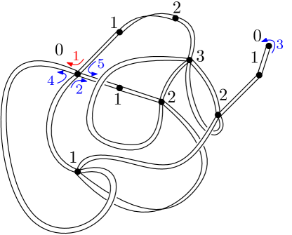
((b))

Figure 1. Left: the local constraints around a vertex of colour $i\in(0,k)$. Right: a labeled $3$-constellation of size $5$, in ribbon-graph representation; the corners of colour $0$ are labeled from $1$ to $5$, and each of them is oriented; disregarding the labels of corners and the orientation of all blue corners (so that there remains only one distinguished and oriented corner, the red one) gives a rooted $3$-constellation (of size $5$).

Definition 2.2 (Constellation, see Figure 1).

Let $k\geq 1$ be an integer. A $k$-constellation is a map, equipped with a coloring of its vertices with colors in $\{0,1,2,\dots,k\}$, such that

1. each vertex colored by $0$ ($k$, respectively) has only neighbours of color $1$ ($k-1$ respectively),

2. for any $0<i<k$ and for any vertex $v$ colored by $i$, each corner of $v$ separates vertices colored by $i-1$ and $i+1$.

The degree of a face in a $k$-constellation is the number of corners of colour $0$ it contains, which is the same as the number of corners of colour $k$, and as half the number of corners of any other colour (the color of a corner is the color of the vertex it is incident to). The degree of a vertex of color $0$ or $k$ in a $k$-constellation is the number of its adjacent corners, while the degree of a vertex of color $i\in[1..k-1]$ in a $k$-constellation is half the number of its adjacent corners. The size of a constellation $\mathbf{M}$ is its number of corners of colour $0$ and is denoted by $|\mathbf{M}|$. In particular any $k$-constellation $\mathbf{M}$ has $k\cdot|\mathbf{M}|$ edges. A constellation of size $n$ is labeled if its corners of colour $0$ are labeled with the integers from $1$ to $n$, and if each such corner carries an (arbitrary) orientation. A constellation is rooted if it is equipped with a distinguished oriented corner of colour $0$, called the root (if the constellation is already labeled, the orientation of the root corner is already given, but for unlabeled maps, this orientation is part of the information given by the rooting). The root vertex (or face, respectively) is the vertex (or face) incident to the root corner. The color of an edge is the pair $\{i,j\}$ formed by the colors of its two endpoints. The full profile of a $k$-constellation is the $k+2$-tuple $(\lambda^{-1},\lambda^{0},\lambda^{1},\dots,\lambda^{k})$, where $\lambda^{-1}$ is the partition encoding face degrees and $\lambda^{i}$ is the partition encoding degrees of vertices of colour $i$.

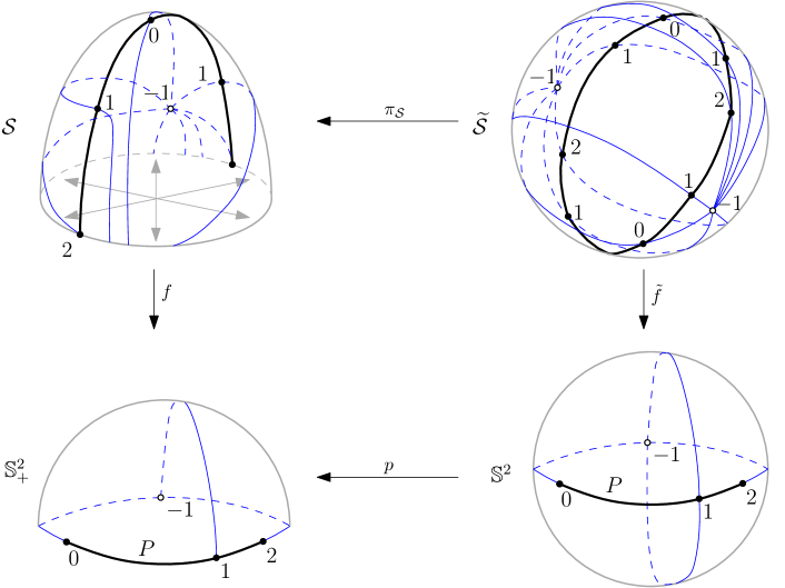
Figure 2. The correspondence between generalized branched coverings and constellations in the case of $k+2=4$ ramification points. The base graph $P$, which is a path, and the corresponding constellations are drawn in fat black. Blue lines give the triangulations described in the proof of Proposition 2.3. On this example, $\widetilde{\mathcal{S}}$ is the sphere and $\mathcal{S}$ is the projective plane and the full profile is given by $((2),(2),(1,1),(2))$.

We can now state the correspondence between coverings and constellations. The proof uses a classical result in the orientable case.

Proposition 2.3 (see Fig. 2-Left).

Let $k\geq 1$ be an integer and let $f:\mathcal{S}\rightarrow\mathbb{S}^{2}_{+}$ be a generalized branched covering of the sphere with $k+2$ ramification points as in Definition 2.1 monotonically numbered from $-1$ to $k$ along the equator $\partial\mathbb{S}^{2}_{+}$. Let $P$ be a path on the equator going through the points $0,1,\dots,k$ in this order. Then the preimage $f^{-1}(P)\subset\mathcal{S}$ is a $k$-constellation on $\mathcal{S}$.

This construction gives a one-to-one correspondence between equivalence classes of generalized branched coverings of the sphere with $k+2$ monotonically numbered ramification points and full profile $(\lambda^{-1},\lambda^{0},\lambda^{1},\dots,\lambda^{k})$, and $k$-constellations with the same full profile.

Proof.

The fact that the embedded graph $f^{-1}(P)$ on $\mathcal{S}$ satisfies the local constraints of constellations (with vertex colours given by the pull-back of the numbering of ramification points) is clear. The fact that it is a well-defined map comes from the fact that each region delimited by this graph on $\mathcal{S}$ retracts to the neighbourhood of a preimage of the ramification point $-1$. Each such neighbourhood is homeomorphic to a disk by definition of a generalized branched covering. We need to prove that $f^{-1}(P)$ gives the same constellation for equivalent generalized coverings. First note that $P$ is naturally identified with $p^{-1}(P)$, since $p$ is the identity on $\partial\mathbb{S}^{2}_{+}=\mathbb{S}^{2}_{+}\cap\mathbb{S}^{2}_{-}$, so we will denote both paths simply by $P$. In particular, using (4) we have $\tilde{f}^{-1}(P)=(p\tilde{f})^{-1}(P)=(f\pi_{S})^{-1}(P)$, which does not depend on the choice of $\widetilde{f}$. This means that the constellation $\tilde{f}^{-1}(P)$ on $\tilde{\mathcal{S}}$ is determined by $f$. It is a standard fact in the orientable case (see [LZ04, Chapter 1], adapted to our slightly different choice of base graph) that the constellation $\tilde{f}^{-1}(P)$ determines $\tilde{f}$ uniquely up to equivalence. Now, let $f$ and $g$ be equivalent generalized coverings, and consider the (unique up to equivalence) associated branched coverings $\tilde{f}$, $\tilde{g}$. By definition $\tilde{f}$ and $\tilde{g}$ are equivalent, therefore $\tilde{f}^{-1}(P)$ and $\tilde{g}^{-1}(P)$ are the same constellations. Using (4) again shows that $f^{-1}(P)=\pi_{S}(\tilde{f}^{-1}(P))$ (and the analogue statement for $g$), therefore the two constellations $f^{-1}(P)$ and $g^{-1}(P)$ are also the same, as we wanted to prove.

Now let $\mathbf{M}$ be a constellation of $\mathcal{S}$. Then $\widetilde{\mathbf{M}}=\pi_{\mathcal{S}}^{-1}(\mathbf{M})$ is a map on the orientable surface $\widetilde{\mathcal{S}}$. Using the standard arguments of the orientable case [LZ04, Chapter 1] (adapted again to our choice of base graph), we can construct from $\tilde{\mathbf{M}}$ a branched covering $\tilde{f}:\widetilde{\mathcal{S}}\rightarrow\mathbb{S}^{2}$ as follows. Triangulate $\mathbb{S}^{2}$ by triangles with vertices given by the ramification points labeled by $-1,i,i-1$ for $i\in[1..k]$. In this way, we obtain $k$ triangles on the upper hemisphere $\mathbb{S}^{2}_{+}$ and $k$ corresponding (through $p$) triangles on the lower hemisphere, and such that the equator $\mathbb{S}^{2}_{+}\cap\mathbb{S}^{2}_{-}$ is a cycle $(-1,0,\dots,k)$, see Fig. 2. Triangulate each face of $\mathbf{M}$ by putting a new vertex $-1$ inside each face and connecting it to all the corners of the corresponding face. Pick an orientation on $\widetilde{\mathcal{S}}$ to send triangles with the set of vertices $-1,i,i-1$ visited in this order to the corresponding triangle in $\mathbb{S}^{2}_{+}$ and visited in the reverse order to the corresponding triangle in $\mathbb{S}^{2}_{-}$. Note that applying $\pi_{\mathcal{S}}$ to the triangulation of $\widetilde{\mathcal{S}}$ we obtain a triangulation of $\mathcal{S}$, which allows us to construct $f$ by sending triangles of the form $-1,i,i-1$ into corresponding triangles in $\mathbb{S}^{2}_{+}$. The compatibility relation $f\circ\pi_{\mathcal{S}}=p\circ\tilde{f}$ is satisfied since the triangulations of $\mathbb{S}^{2}_{+}$ and $\mathbb{S}^{2}_{-}$ are identified by $p$.

The fact that the two constructions are inverse of each other, and that the full profile is preserved, is direct by construction. ∎

We remark that the Euler characteristic $\chi(\mathcal{S})$ of the covering surface can be recovered from the full profile $(\lambda^{-1},\dots,\lambda^{k})$ via the Riemann-Hurwitz/Euler formula:

(5) $$\chi(\mathcal{S})=2n-\sum_{i=-1}^{k}(n-\ell(\lambda^{i})).$$

Indeed, this formula is true for branched coverings and by construction this immediately implies that it holds for generalized branched coverings as well. We remark that (5) only involves the length of each partition $\lambda^{i}$. In this paper we will enumerate generalized branched coverings of the sphere without controlling the full profile, but with enough control to keep track of these lengths, hence of the Euler characteristic of the underlying surface.

Remark 1.

Now that the correspondence between generalized branched coverings and constellations is established, in the rest of the paper, we will work with $k$-constellations, which are more convenient to enumerative purposes. The theorem stated in the introduction (Theorem 1.1) will be proved in the language of constellations (Theorem 5.10). The sum over rooted coverings $f$ in this theorem is understood as the sum over rooted constellations $(\mathbf{M},c)$ in (54). The integer parameter $\nu_{\rho}(f)$ in that theorem is understood as the parameter $\nu_{\rho}(\mathbf{M},c)$ that we introduce in the next section, while the quantities $|f|,\kappa(f),v_{i}(f)$ in the theorem are understood respectively as the quantities $|\mathbf{M}|,\kappa(\mathbf{M},c),v_{i}(\mathbf{M})$ defined in Section 2 and Section 3.

Remark 2.

Some authors may prefer to call $(k+1)$-constellations what we call $k$-constellations here. This is related to the fact that in our main function (2) we have two sets of “time” parameters $\mathbf{p}$ and $\mathbf{q}$. In many applications one studies the specialization $q_{i}=\mathbf{1}_{i=1}$, which on coverings corresponds to the case where the second marked ramification point is trivial (this is the same as viewing single Hurwitz numbers as special cases of double ones). Among these two natural choices of terminology, we kept the one that was shorter and more convenient for our purposes.

We conclude this section by introducing the notion of duality.

Definition 2.4.

Duality is the involution on $k$-constellations defined as follows. Given a $k$-constellation $\mathbf{M}$, add a new vertex of colour $-1$ inside each face and link it by a new edge to all corners of label $k$. Then remove all vertices of $\mathbf{M}$ of colour $0$ and edges incident to them. Finally, exchange colours $-1\leftrightarrow 0$ and $k+1-i\leftrightarrow i$ for each $1\leq i\leq k$. The map $\tilde{\mathbf{M}}$ thus obtained is called the dual of $\mathbf{M}$.

The fact that duality is an involution is clear from the interpretation on coverings, since it can be interpreted as a reflection of $\mathbb{S}^{2}_{+}$ together with a renumbering of ramification points. There is a natural correspondence between corners of colour $0$ in $\mathbf{M}$ and $\tilde{\mathbf{M}}$, which enables to lift duality at the level of labeled and/or rooted objects. Indeed, let $\mathbf{M}^{\prime}$ be an intermediate map constructed from $\mathbf{M}$ by adding a new vertex of colour $-1$ inside each face and linking it by a new edge to all corners of label $k$. Note that each face of $\mathbf{M}^{\prime}$ contains precisely one corner of color $-1$ and one corner of color $0$. In particular orienting this face is equivalent to orienting the corresponding corner of color $-1$ and it is also equivalent to orienting the corresponding corner of color $0$.

3. MON’s and the $b$-deformed decomposition equation

3.1. MON’s and weights

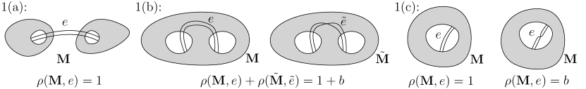
Figure 3. The main axioms of MONs.

Our way to assign a $b$-dependent weight to a map proceeds by repeated edge-deletions. The weight attached to each deletion depends on a number of arbitrary choices subject to suitable axioms, encompassed by the concept of measure of non-orientability.

Definition 3.1 (MON; see Fig. 3).

A measure of non-orientability (MON) is a function $\rho(\cdot,\cdot)$ with value in $\mathbb{Q}[b]$ that associates to a vertex-colored map $\mathbf{M}$ and an edge $e$ in $\mathbf{M}$, some value $\rho(\mathbf{M},e)$ and that satisfies the following properties.

1. Let $\mathbf{N}:=\mathbf{M}\setminus\{e\}$ and let $c_{1},c_{2}$ be the two corners delimited by the endpoints of $e$ in $\mathbf{N}$.

   1. If $c_{1},c_{2}$ belong to two distinct connected components of $\mathbf{N}$, then $\rho(\mathbf{M},e)=1$.

   2. If $c_{1},c_{2}$ belong to the same connected component of $\mathbf{N}$ but to two different faces, then let $\tilde{e}$ be the other edge that could be added to $\mathbf{N}$ between these corners to form a new map $\tilde{\mathbf{M}}$. Then $\rho(\mathbf{M},e)+\rho(\tilde{\mathbf{M}},\tilde{e})=1+b$.

   3. If $c_{1},c_{2}$ belong to the same face of $\mathbf{N}$, then $\rho(\mathbf{M},e)=1$ if $e$ splits this face into two faces (“untwisted diagonal)” and $\rho(\mathbf{M},e)=b$ otherwise (“twisted diagonal”).

2. the value of $\rho(\mathbf{M},e)$ depends only on the connected component of $\mathbf{M}$ containing $e$.

If $e_{1},e_{2},\dots,e_{i}$ are edges of $\mathbf{M}$, we will denote

$$\rho(\mathbf{M};e_{1},\dots,e_{i}):=\rho(\mathbf{M},e_{1})\rho(\mathbf{M}\setminus\{e_{1}\},e_{2})\dots\rho(\mathbf{M}\setminus\{e_{1},\dots,e_{i-1}\},e_{i}).$$

This quantity in general depends on the ordering of the edges $e_{1},\dots,e_{i}$. We will also use the notation $\rho(\mathbf{M};L)$ where $L=(e_{1},\dots,e_{i})$ is an ordered list of edges.

Example 1.

Let us compute the value of $\rho(\mathbf{M};e_{1},e_{2},e_{3})$ for the three examples of Figure 4. In case a), both $\mathbf{M}$ and $\mathbf{M}\setminus\{e_{1}\}$ have one face, therefore $e_{1}$ is a “twisted diagonal” and $\rho(\mathbf{M};e_{1})=b$ by condition 1c) of Definition 3.1. Removing $e_{2}$ from $\mathbf{M}\setminus\{e_{1}\}$ also produces a map with one face, so this is again the same case and $\rho(\mathbf{M};e_{1},e_{2})=b^{2}$. Finally removing $e_{3}$ from $\mathbf{M}\setminus\{e_{1},e_{2}\}$ disconnects this map, so we are in case 1a), and finally $\rho(\mathbf{M};e_{1},e_{2},e_{3})=b^{2}$. The labeled map in case b) is identical to the one in case a), but the order of edge removals is different. The removal of $e_{1}$ from $\mathbf{M}$ produces a map with two faces, therefore we are in case 1b) and $\rho(\mathbf{M},e_{1})$ can be a priori any polynomial $X\in\mathbb{Q}[b]$. However, we need to remember that 1b) says there exists a labeled map $\tilde{\mathbf{M}}$ and an edge $e_{1}$ (shown in case c) ) such that $\rho(\tilde{\mathbf{M}},e_{1})=1+b-X$. Removing the edge $e_{2}$ from $\mathbf{M}\setminus\{e_{1}\}$ (which is the same map as $\tilde{\mathbf{M}}\setminus\{e_{1}\}$) produces a map whose number of faces is smaller by one, therefore this edge is an “untwisted diagonal”, which gives from 1c) $\rho(\mathbf{M};e_{1},e_{2})=X$ and $\rho(\tilde{\mathbf{M}};e_{1},e_{2})=1+b-X$. Removing the last edge corresponds to case 1a) and therefore $\rho(\mathbf{M};e_{1},e_{2},e_{3})=X$ and $\rho(\tilde{\mathbf{M}};e_{1},e_{2},e_{3})=1+b-X$. Finally, note that the map $\tilde{\mathbf{M}}$ from case c) is orientable. If we assume that $\rho$ is integral (Definition 3.2), we have necessarily $X=b$, imposing $\rho(\tilde{\mathbf{M}};e_{1},e_{2},e_{3})=1$, and $\rho(\mathbf{M};e_{1},e_{2},e_{3})=b$ for the map $\mathbf{M}$ from case b).

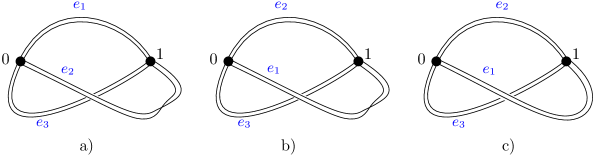
Figure 4. Three maps $\mathbf{M}$ with edges labeled $e_{1},e_{2},e_{3}$. See Example 1 for the computation of $\rho(\mathbf{M};e_{1},e_{2},e_{3})$ in each case.

Our main results also require us to define integral and coherent MONs.

Definition 3.2 (Integral MON, Coherent MON; see Fig. 5).

A MON $\rho$ is integral if $\rho(\mathbf{M},e)$ belongs to $\{1,b\}$ for any $\mathbf{M}$ and $e$, and if the following is true: for every pair $(\mathbf{M},e)$ which is in case (1)(b) of Definition 3.1 and such that $\mathbf{M}$ is orientable, we have $\rho(\mathbf{M},e)=1$ and $\rho(\tilde{\mathbf{M}},\tilde{e})=b$, in the notation of Definition 3.1.

A MON $\rho$ is coherent if for any colored map $\mathbf{M}$, for any corner $c$ of $\mathbf{M}$ of color $j$, and for any face $f$ of $\mathbf{M}$ having an even number of corners of color $j+1$, the following is true. Choose an arbitrary orientation of $f$, and number $c_{1},\dots,c_{2d}$ the corners of color $j+1$ in $f$ (these corners inherit the orientation of $f$). Also choose an arbitrary orientation for $c$. For $i\in[1..2d]$ let $e_{i},\tilde{e}_{i}$ be the two possible edges connecting $c$ to $c_{i}$, where $e_{i}$ is the one that respect the corner orientations, and $\tilde{e}_{i}$ is its twist. Then for any $i$:

$$\rho(\mathbf{M}\cup\{e_{i}\},e_{i})+\rho(\mathbf{M}\cup\{\tilde{e}_{i+1}\},\tilde{e}_{i+1})=(1+b)$$

with the convention that $\tilde{e}_{2d+1}:=\tilde{e}_{1}$.

The idea of using MON’s or their variants already appeared in previous works on the $b$-conjecture at least since Lacroix [La 09] (see also [DFS14, Doł17]). Here we have added Axiom (2) which is necessary for the generating function arguments in the next section. Note also that previous authors only consider what we call here integral MON’s. Although considering non-integrals MON’s is not needed strictly speaking for this paper, we believe that this is natural and may be useful for further developments (see Remark 3 below).

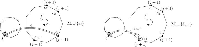
Figure 5. A coherent MON: $\rho(\mathbf{M}\cup\{e_{i}\},e_{i})+\rho(\mathbf{M}\cup\{\tilde{e}_{i+1}\},\tilde{e}_{i+1})=(1+b).$

It is easy to see that MONs exist and to construct them. In fact, we have

Lemma 3.3.

There exist MONs that are both coherent and integral.

Proof.

The only choices that we have to make to construct a MON are the values of $\rho(\mathbf{M},e)$ and $\rho(\tilde{\mathbf{M}},\tilde{e})$ for pairs $(\mathbf{M},e)$ that are in case 1(b) of Definition 3.1. Indeed, all other values are imposed by the axioms. If we only wanted to respect Axiom (1), we could choose these values arbitrarily in $\{1,b\}$. Here we also have to be careful to perform these choices simultaneously to respect Axiom (2) and to ensure coherence and integrality. For this we adapt the arguments of [Doł17, Section 5.1] to our settings.

We first equip every connected vertex-coloured map with a fixed orientation of all its faces, given by a global orientation if the surface is orientable, and chosen arbitrarily for each face otherwise. Given an edge $e$ in a vertex-coloured map $\mathbf{M}$ such that the pair $(\mathbf{M},e)$ is in case 1(b) of Definition 3.1, we let $\mathbf{N}$ be the connected component of $\mathbf{M}$ containing $e$. Removing $e$ from $\mathbf{N}$ creates a smaller map with two marked corners. We let $\rho(M,e)=1$ if the edge $e$ respects the fixed orientation of these corners, and $\rho(M,e)=b$ otherwise. By construction this choice respects Axiom (2). Coherence is clear, because the edges $e_{i}$ and $\tilde{e}_{i+1}$ in Definition 3.2 have opposite conventional orientations along their faces and therefore are associated with the two values $1$ and $b$ (in some order). The fact that this MON is integral comes from the fact that we have chosen the orientation of faces from a global surface orientation whenever the map is orientable. ∎

Remark 3.

We can construct a MON by choosing the two values in case 1(b) of Definition 3.1 to be both equal to $(1+b)/2$. We obtain a MON denoted by $\rho_{SYM}$, which is not integral, but is coherent. Introducing $\rho_{SYM}$ is not necessary, strictly speaking, to prove the results of this paper, but it played a role in our discovery of the “heuristic proofs” given in Section 4.4. Also, since we prove in this paper that the $b$-weighted enumeration of constellations is independent of the choice of a coherent MON (Corollary 3.12 page 3.12), it is natural to expect that further works on the subject use the possibility to work with the coherent MON $\rho_{SYM}$, which is simple and canonical.

3.2. Right-paths and the combinatorial decomposition

Definition 3.4 (Right-path).

(see Fig. 6) Let $\mathbf{M}$ be a $k$-constellation and $c$ be an oriented corner of color $0$ in $\mathbf{M}$, lying in some face $f$. The sequence of $k$ edges $e_{1},e_{2},\dots,e_{k}$ that follow $c$ around $f$, in the orientation of $c$, is called the right-path of $c$. Note that the edge $e_{i}$ has color $\{i-1,i\}$.

Figure 6. The $3$-constellation of Fig. 1. The right-path $(e_{1},e_{2},e_{3})$ of the (oriented) root is shown in (bold) red. In (dotted) green, we show the right-path $(e_{1}^{\prime},e_{2}^{\prime},e_{3}^{\prime})$ of the same corner but with opposite orientation.

From the local coloring constraints that define $k$-constellations, we clearly have:

Lemma 3.5.

If $\mathbf{M}$ is a $k$-constellation and $P$ is a right-path in $\mathbf{M}$, then $\mathbf{M}\setminus P$ is again a $k$-constellation (with possibly more connected components than $\mathbf{M}$).

We now introduce the combinatorial decompositionwhich consists in removing right-paths recursively from a connected $k$-constellation until the whole map has been exhausted.

In this definition we assume that some underlying MON $\rho$ has been fixed.

Definition 3.6 (Combinatorial decomposition).

Let $(\mathbf{M},c)$ be a rooted connected $k$-constellation. The combinatorial decomposition of $(\mathbf{M},c)$ is the recursive algorithm defined as follows:

• We let $\mathbf{M}_{0}=\mathbf{M}$ and we let $c_{0}:=c$, $m:=\deg(v(c))$, where $v(c)$ is the vertex adjacent to $c$ (the root vertex of $\mathbf{M}$);

• For each $i$ from $1$ to $m$, we let $P_{i}=(e^{(i)}_{1},e^{(i)}_{2},\dots,e^{(i)}_{k})$ be the right-path of the corner $c_{i-1}$ in $\mathbf{M}_{i-1}$. We let $\mathbf{M}_{i}:=\mathbf{M}_{i-1}\setminus P_{i}$. For $i<m$ we let $c_{i}$ be the oriented corner induced by $c_{i-1}$ in the map $\mathbf{M}_{i}$.

• We let $L$ be the ordered list of edges

  $$L=(e^{(1)}_{1},e^{(1)}_{2},\dots,e^{(1)}_{k},e^{(2)}_{1},e^{(2)}_{2},\dots,e^{(2)}_{k},\dots,\dots,e^{(m)}_{1},e^{(m)}_{2},\dots,e^{(m)}_{k}).$$

  We say that the weight $\rho(\mathbf{M};L)$ has been collected by the algorithm.

• If the map $\mathbf{M}_{m}$ is empty, then stop. If it is not, let $\mathbf{M}^{(1)},\dots,\mathbf{M}^{(i)}$ be its connected components. For $j\in[1..i]$ let $c^{(j)}$ be the last corner in $\mathbf{M}^{(j)}$ from which an edge was deleted in the execution of the algorithm (in other terms after removing an edge attached to $c^{(j)}$ in the execution of the algorithm no other edge was removed from $\mathbf{M}^{(j)}$). This corner naturally inherits the orientation of the last right-path removed from it. We root $\mathbf{M}^{(j)}$ in the first corner of color $0$ following the oriented corner $c^{(j)}$ (that is to say, we visit consecutive corners of the face of $\mathbf{M}^{(j)}$ which contains $c^{(j)}$ starting from this corner and following its orientation, until a corner of colour $0$ is reached, and we take that corner as the root). Let $\tilde{\mathbf{M}}^{(1)},\dots,\tilde{\mathbf{M}}^{(i)}$ be their dual maps.

• Run recursively the algorithm on each of the maps $\tilde{\mathbf{M}}^{(1)},\dots,\tilde{\mathbf{M}}^{(i)}$.

Fig. 7 shows the combinatorial decomposition of the $3$-constellation from Fig. 1(b). The need to alternate between primal and dual maps in the decomposition may seem unnatural to the reader. As we will see, it comes from the fact that the differential equations we use to make the connection with Jack polynomials mix two sets of differential variables ($\mathbf{p}$ and $\mathbf{q}$, see Proposition 5.8).

Definition 3.7.

Fix a MON $\rho$, and let $(\mathbf{M},c)$ be a rooted connected $k$-constellation. We define the weight $\vec{\rho}(\mathbf{M},c)$ of $(\mathbf{M},c)$ as the product of all the weights collected during the combinatorial decomposition of $(\mathbf{M},c)$.

Example 2.

Let us compute $\vec{\rho}(\mathbf{M},c)$ for the rooted map $(\mathbf{M},c)$ of Fig. 1(b). During the combinatorial decomposition we first remove four right-paths attached to the root vertex, until the 3-constellation $\mathbf{M}_{4}$ has more than one connected component (it has two: the trivial one consisting of the root vertex and $\mathbf{M}^{(1)}$ shown in Fig. 7). The edges appearing in the list $L$ produced by the combinatorial decomposition are depicted in Fig. 7. One can check that $\rho(\mathbf{M}_{0},P_{1})=X_{1}\cdot X_{2}\cdot 1$, $\rho(\mathbf{M}_{1},P_{2})=1\cdot 1\cdot b$, $\rho(\mathbf{M}_{2},P_{3})=b\cdot 1\cdot 1$, $\rho(\mathbf{M}_{3},P_{4})=1\cdot 1\cdot 1$, where $X_{1},X_{2}\in\mathbb{Q}[b]$ are fixed polynomials associated with $\rho$ by Axiom 1b) of Definition 3.1 (the $i$-th term in the product expressing $\rho(\mathbf{M}_{j-1},P_{j})$ corresponds to removing $e^{(j)}_{i}$). In particular $\rho(\mathbf{M},L)=b^{2}\cdot X_{1}\cdot X_{2}$. Finally, $\rho(\tilde{\mathbf{M}}^{(1)})=1\cdot 1\cdot 1$ so that $\vec{\rho}(\mathbf{M},c)=b^{2}\cdot X_{1}\cdot X_{2}$.

Figure 7. Combinatorial decomposition of the $3$-constellation from Fig. 1(b). In the left we indicate which edges of $\mathbf{M}$ are listed in the first part of the algorithm. Red oriented corners show how to root the connected component $\mathbf{M}^{(1)}$ by first orienting the corner $c^{(1)}$ and following its orientation until we reach the first corner of color $0$. On the right hand side the red vertex and the red edge are not part of $\mathbf{M}^{(1)}$ but they indicate the intermediate step of the construction of the dual map $\tilde{\mathbf{M}}^{(1)}$, which also shows how to orient the root of $\tilde{\mathbf{M}}^{(1)}$ (see Definition 2.4 and the comment following it).

Definition-Lemma 3.8.

Let $\rho$ be an integral MON, and let $(M,c)$ be a connected rooted $k$-constellation. Then we have

$$\vec{\rho}(\mathbf{M},c)=b^{\nu_{\rho}(\mathbf{M},c)},$$

where $\nu_{\rho}(\mathbf{M},c)$ is a nonnegative integer, which is zero if and only if $\mathbf{M}$ is orientable.

Proof.

The fact that $\vec{\rho}(\mathbf{M},c)$ is a monomial is a direct consequence of the definitions. The fact that $\nu_{\rho}(\mathbf{M},c)$ is zero if and only if $\mathbf{M}$ is orientable follows from the fact that it is orientable if and only if the weight $1$ (instead of $b$) is collected at each step of the combinatorial decomposition, which is clear by inspecting all cases in the definition of a MON. ∎

3.3. $b$-weights and $p_{\cdot}q_{\cdot}u_{\cdot}y_{\cdot}$-markings

In this paper we will consider generating functions of constellations, and we will be able to keep track of many parameters of these combinatorial objects in our formulas. In order to make our discussions as clear and readable as possible, we fix some terminology and notation now.

To a constellation $\mathbf{M}$ (possibly rooted, or labeled), we will associate several sorts of “weights”:

• a $b$-weight, which is a quantity in $\mathbb{Q}[b]$, a priori dependent on the choice of an underlying MON $\rho$. Example of $b$-weights are the quantities $\vec{\rho}(\mathbf{M},c)$ or $b^{\nu_{\rho}(\mathbf{M},c)}$ defined above. We will restrict the word weight to these quantities.

• a monomial weight in the variables $p_{i},q_{i},u_{i},y_{i}$, which serves as a marking keeping track of parameters of the map, such as the face or vertex degrees. To avoid confusion with the $b$-weights we will use the word marking instead of weight for these quantities.

For the rest of this paper we fix indeterminates $b$, $\mathbf{p}=(p_{i})_{i\geq 1}$, $\mathbf{q}=(q_{i})_{i\geq 1}$, $\bm{y}=(y_{i})_{i\geq 0}$, $\bm{u}=(u_{i})_{i\geq 1}$. If $\mathbf{M}$ is a constellation we denote by $cc(\mathbf{M})$ its number of connected components, and by $F(\mathbf{M})$ the set of its faces. For $i\geq 0$ we denote by $V_{i}(\mathbf{M})$ the set of vertices of color $i$ and by $v_{i}(\mathbf{M})$ its cardinality. Recall also that $|\mathbf{M}|$ is the size, i.e. the number of corners of colour $0$, of $\mathbf{M}$.

Definition 3.9 (Markings).

Let $\mathbf{M}$ be a $k$-constellation. The marking of $\mathbf{M}$ is the monomial

(6) $$\kappa(\mathbf{M}):=\prod_{f\in F(\mathbf{M})}p_{\deg(f)}\prod_{v\in V_{0}(\mathbf{M})}q_{\deg(v)}\prod_{i=1}^{k}u_{i}^{v_{i}(\mathbf{M})}.$$

Let $(\mathbf{M},c)$ be a rooted $k$-constellation, and $f_{c}$ be its root face. The marking of $(\mathbf{M},c)$ is the monomial

$$\vec{\kappa}(\mathbf{M},c):=y_{\deg(f_{c})}\prod_{f\in F(\mathbf{M})\setminus\{f_{c}\}}p_{\deg(f)}\prod_{v\in V_{0}(\mathbf{M})}q_{\deg(v)}\prod_{i=1}^{k}u_{i}^{v_{i}(\mathbf{M})}=\frac{y_{\deg(f_{c})}}{p_{\deg(f_{c})}}\kappa(\mathbf{M}).$$

In other words, our marking uses variables $p_{i}$ to record a non-root face of degree $i$, $q_{i}$ to record a vertex of colour $0$ and degree $i$, variables $u_{i}$ to record a vertex of color $i$, and $y_{i}$ to record the fact that the root face has degree $i$.

Example 3.

For the rooted $3$-constellation from Fig. 1(b) one has $\vec{\kappa}(\mathbf{M},c)=y_{5}\cdot q_{4}\cdot q_{1}\cdot u_{1}^{4}\cdot u_{2}^{3}\cdot u_{3}$.

3.4. Generating functions of connected maps and the decomposition equations.

Let $\rho$ be a MON. We let $\vec{H}_{\rho}(t;\mathbf{p},\mathbf{q},\bm{y},u_{1},\dots,u_{k})$ be the multivariate generating function of rooted connected $k$-constellations given by the formula

(7) $$\vec{H}_{\rho}(t;\mathbf{p},\mathbf{q},\bm{y},u_{1},\dots,u_{k}):=\sum_{n\geq 1}\sum_{(\mathbf{M},c)}t^{n}\vec{\rho}(\mathbf{M},c)\vec{\kappa}(\mathbf{M},c),$$

where the second sum is taken over rooted connected (unlabeled) $k$-constellations of size $n$. Formally $\vec{H}_{\rho}$ is viewed as formal power series in $t$, with coefficients that are polynomials in the variables $y_{i},p_{i},q_{i},u_{i}$, with coefficients in $\mathbb{Q}(b)$, that is

$$\vec{H}_{\rho}\in\mathbb{Q}(b)[\bm{y},\mathbf{p},\mathbf{q},u_{1},\dots,u_{k}][[t]].$$

For $m\geq 1$, we also denote by $\vec{H}_{\rho}^{[m]}$ the contribution to $\vec{H}_{\rho}$ of maps whose root vertex has degree $m$

(8) $$\vec{H}_{\rho}^{[m]}(t;\mathbf{p},\mathbf{q},\bm{y},u_{1},\dots,u_{k}):=q_{m}^{-1}\sum_{n\geq 1}\sum_{(\mathbf{M},c)\atop\deg v_{c}=m}t^{n}\vec{\rho}(\mathbf{M},c)\vec{\kappa}(\mathbf{M},c),$$

where the second sum is now taken over rooted connected (unlabeled) $k$-constellations of size $n$ whose root vertex $v_{c}$ has degree $m$. Note that we do not count the root vertex in the marking (hence the factor $q_{m}^{-1}$). By definition one has:

(9) $$\vec{H}_{\rho}=\sum_{m\geq 1}q_{m}\cdot\vec{H}_{\rho}^{[m]}.$$

We also consider the variant where the root face is marked with $\mathbf{p}$-variables, namely

$$H_{\rho}^{[m]}=\Theta_{Y}\vec{H}_{\rho}^{[m]}=q_{m}^{-1}\sum_{n\geq 1}\sum_{(\mathbf{M},c)\atop\deg v_{c}=m}t^{n}\vec{\rho}(\mathbf{M},c)\kappa(\mathbf{M}),$$

with

(10) $$\Theta_{Y} :=\sum_{i\geq 1}p_{i}\frac{\partial}{\partial y_{i}}.$$

Finally, we let $\pi$ be the operator that exchanges the sets of variables $\mathbf{p}\leftrightarrow\mathbf{q}$ and $u_{i}\leftrightarrow u_{k+1-i}$ for $1\leq i\leq k$, and we let

(11) $$\widetilde{H}_{\rho}^{[m]}:=\pi H_{\rho}^{[m]}.$$

Note that, by applying duality, we have

(12) $$\widetilde{H}_{\rho}^{[m]}=p_{m}^{-1}\sum_{n\geq 1}\sum_{(\mathbf{M},c)\atop\deg f_{c}=m}t^{n}\vec{\rho}{(\tilde{\mathbf{M}},\tilde{c})}\kappa(\mathbf{M}),$$

where the second sum is now taken over rooted connected (unlabeled) $k$-constellations of size $n$ whose root face has degree $m$. Note that in this sum the $b$-weight is computed on the dual rooted map $(\tilde{\mathbf{M}},\tilde{c})$ of $(\mathbf{M},c)$, and that we used that $\kappa(\tilde{\mathbf{M}})=\pi\kappa(\mathbf{M})$.

We will now state a set of equations (which we call “decomposition equations”) that characterizes these functions. We first need to define some operators:

$$\Lambda_{Y} :=(1+b)\sum_{i,j\geq 1}y_{i+j-1}\frac{i\partial^{2}}{\partial p_{i}\partial y_{j-1}}+\sum_{i,j\geq 1}y_{i-1}p_{j}\frac{\partial}{\partial y_{i+j-1}}+b\cdot\sum_{i\geq 0}y_{i}\frac{i\partial}{\partial y_{i}},$$

$$Y_{+} :=\sum_{i\geq 0}y_{i+1}\frac{\partial}{\partial y_{i}}.$$

Theorem 3.10 (Decomposition equations).

Let $\rho$ be any coherent MON. Then the family of generating series $\vec{H}_{\rho}^{[m]}\equiv\vec{H}_{\rho}^{[m]}(t;\mathbf{p},\mathbf{q},\bm{y},u_{1},\dots,u_{k})$ satisfies the following set of equations, for $m\geq 1$:

(13) $$\vec{H}_{\rho}^{[m]}=t^{m}\cdot\Big{(}Y_{+}\prod_{l=1}^{k}\big{(}\Lambda_{Y}+u_{l}+\sum_{i,j\geq 1}y_{j+i-1}\widetilde{H}_{\rho}^{[i]}\frac{\partial}{\partial y_{j-1}}\big{)}\Big{)}^{m}(y_{0}).$$

Corollary 3.11.

Let $\rho$ be any coherent MON. Then the family of generating series $(H_{\rho}^{[m]})_{m\geq 1}$ is fully characterized by the following set of equations, for $m\geq 1$:

(14) $$H_{\rho}^{[m]}(t;\mathbf{p},\mathbf{q},u_{1},\dots,u_{k})=t^{m}\cdot\Theta_{Y}\Big{(}Y_{+}\prod_{l=1}^{k}\big{(}\Lambda_{Y}+u_{l}+\sum_{i,j\geq 1}y_{j+i-1}\widetilde{H}_{\rho}^{[i]}\frac{\partial}{\partial y_{j-1}}\big{)}\Big{)}^{m}(y_{0}),$$

together with (11).

Proof of the corollary.

Equation (13) implies (14) by applying the operator $\Theta_{Y}$ to both sides. It is clear that this set of equations characterizes the functions since coefficients can be computed inductively from the equations, order by order in $t$. ∎

In particular, we observe that

Corollary 3.12.

The functions $\vec{H}_{\rho}$, $H_{\rho}^{[m]}$, $\widetilde{H}_{\rho}^{[m]}$ do not depend on the coherent MON $\rho$.

3.5. Unconnected functions

Let us consider the following antiderivative of $\Theta_{Y}\vec{H}_{\rho}$:

$$H_{\rho}:=\sum_{n\geq 1}\frac{1}{n}\sum_{(\mathbf{M},c)}t^{n}\vec{\rho}(\mathbf{M},c)\kappa(\mathbf{M}),$$

where the second sum is taken over rooted connected (unlabeled) $k$-constellations of size $n$ so that

$$t\frac{\partial}{\partial t}H_{\rho}=\Theta_{Y}\vec{H}_{\rho}.$$

Then the series $F_{\rho}$ is defined by

$$F_{\rho}=\exp\frac{1}{1+b}H_{\rho}.$$

Note that by Corollary 3.12 it does not depend on the coherent MON $\rho$ and the following identity holds

(15) $$(1+b)t\frac{\partial}{\partial t}\ln F_{\rho}=\Theta_{Y}\vec{H}_{\rho}.$$

We now want to give a combinatorial interpretation to coefficients of $F_{\rho}$. Because each connected rooted constellation has $n!2^{n-1}$ different labellings, we can also write

$$H_{\rho}=\sum_{n\geq 1}\frac{1}{n}\sum_{(\mathbf{M},c)}\frac{t^{n}}{2^{n-1}n!}\vec{\rho}(\mathbf{M},c)\kappa(\mathbf{M})$$

where the second sum is now taken over labeled and rooted connected $k$-constellations of size $n$. This can also be rewritten

$$H_{\rho}=\sum_{n\geq 1}\sum_{\mathbf{M}}\frac{t^{n}}{2^{n-1}n!}\kappa(\mathbf{M})\cdot\mathbf{E}_{c\in\mathbf{M}}[\vec{\rho}(\mathbf{M},c)],$$

where the second sum is now taken over labeled (but no more rooted) connected $k$-constellations of size $n$, and where $\mathbf{E}_{c\in\mathbf{M}}$ now denotes expectation with respect to a corner $c$ of colour $0$ chosen uniformly at random among those of $\mathbf{M}$.

Definition 3.13.

Define the weight of a labeled connected constellation $\mathbf{M}$ as $\tilde{\rho}(\mathbf{M}):=\mathbf{E}_{c\in\mathbf{M}}[\vec{\rho}(\mathbf{M},c)]$. Extend this definition multiplicatively to unconnected (but still labeled) constellations.

Because $\tilde{\rho}(\mathbf{M})$ is multiplicative on connected components by definition, and $\kappa(\mathbf{M})$ and $2^{|\mathbf{M}|-cc(\mathbf{M})}$ also are, the generating function $F_{\rho}=\exp\frac{1}{1+b}H_{\rho}$ can be directly interpreted as the generating function of unconnected objects with these markings. More precisely:

Theorem 3.14.

The generating function $F_{\rho}\equiv F_{\rho}(t;\mathbf{p},\mathbf{q},u_{1},\dots,u_{k})$ defined by (15) is given by the expansion:

(16) $$F_{\rho}=1+\sum_{n\geq 1}\sum_{\mathbf{M}}\frac{t^{n}}{2^{n-cc(\mathbf{M})}n!}\frac{\tilde{\rho}(\mathbf{M})\kappa(\mathbf{M})}{(1+b)^{cc(\mathbf{M})}},$$

where the second sum is taken over labeled $k$-constellations of size $n$, connected or not.

Remark 4.

We will prove (Theorem 5.10) that $F_{\rho}$ is in fact equal to the function $\tau^{(k)}_{b}$ defined in (2). Thus the last theorem gives an explicit interpretation of the coefficients of $\tau^{(k)}_{b}$. We will also show (Lemma 5.7) that $F_{\rho}=\tau^{(k)}_{b}$ satisfies the following equation

(17) $$m\frac{q_{m}\partial}{\partial q_{m}}F_{\rho}(t;\mathbf{p},\mathbf{q},u_{1},\dots,u_{k})=\Theta_{Y}t^{m}\cdot q_{m}\cdot\big{(}Y_{+}\prod_{l=1}^{k}(\Lambda_{Y}+u_{l})\big{)}^{m}\frac{y_{0}}{1+b}F_{\rho}(t;\mathbf{p},\mathbf{q},u_{1},\dots,u_{k}),$$

and similarly, in Corollary 5.9, we will show that

$$m\frac{\partial}{\partial q_{m}}H_{\rho}=H_{\rho}^{[m]}.$$

This equation has the following interpretation. Fix a monomial $\mathbf{m}=p_{\lambda}q_{\mu}u_{1}^{v_{1}}\dots u_{k}^{v_{k}}$ such that the number of parts in $\mu$ equal to $m$ is nonzero, and that there exists at least one connected $k$-constellation with marking $\mathbf{m}$. Then, if $\mathbf{M}$ denotes a random connected $k$-constellation such that $\kappa(\mathbf{M})=\mathbf{m}$, chosen uniformly at random, one has

$$\mathbf{E}_{\mathbf{M}}\mathbf{E}_{c\in\mathbf{M}}[\vec{\rho}(\mathbf{M},c)]=\mathbf{E}_{\mathbf{M}}\mathbf{E}_{c\in\mathbf{M}}[\vec{\rho}(\mathbf{M},c)|\deg v_{c}=m].$$

This “symmetry” is not directly apparent on the combinatorial model.

Remark 5 (Other relations and deformed Virasoro constraints).

In the special cases of $b\in\{0,1\}$ we can obtain other equations, which do not involve differential operators with respect to the variables $(q_{i})_{i\geq 1}$. Indeed, it follows from our proofs that for $b\in\{0,1\}$, one has

(18) $$\frac{\ell\partial}{\partial p_{\ell}}F_{\rho}=[y_{\ell}]\sum_{m\geq 1}t^{m}\cdot q_{m}\cdot\big{(}Y_{+}\prod_{l=1}^{k}(\Lambda_{Y}+u_{l})\big{)}^{m}\frac{y_{0}}{1+b}F_{\rho},$$

where $[y_{\ell}]$ is coefficient extraction. Indeed, our proofs show that the right-hand side is the generating function of rooted constellations in which the root face has degree $\ell$, without attributing any marking to that face (this follows from the combinatorial interpretation of operators given below, which in the case $b\in\{0,1\}$ can be applied also to the combinatorial decomposition of the root component in a rooted unconnected constellation). Such maps can also be obtained by distinguishing a face of degree $\ell$ in an unrooted constellation and choosing one of the $\ell$ corners of colour $0$ it contains as the root, giving rise to the expression of the left-hand side (note that for $b\not\in\{0,1\}$ this argument would not work, since the $b$-weight attributed to a map depends on the choice of the root corner). In the special case $q_{i}=\delta_{1,i}$ and $k=2$, Equation (18) is precisely the $\ell$-th Virasoro constraint for dessins d’enfants for $b=0$ (or its non-orientable generalisation for $b=1$), see [KZ15]. In the general case, possible $b$-analogues of the differential equations (18) and their links with the Virasoro algebra and its central extensions deserve further interest and will be studied in further works.

4. Differential operators: partial right-paths and commutation relations

4.1. Interpretation of the operator $\Lambda_{Y}$ and proof of the decomposition equation

Figure 8. A partial right-path as in Definition 4.1. Black edges belong to a $k$-constellation $\mathbf{N}$, and red edges form a partial right-path $P_{j}$. In the case $j=k$, the color $j+1$ should be replaced by $j-1=k-1$ on the illustration. The blue vertex of color $j-1$ corresponds to the vertex described in the last axiom of the definition, and the blue corners corresponds to the tour of the face $f_{0}$ which determines this blue vertex. Note that, for $j<k$, if one replaced the edge $e_{j}$ by its twist, the configuration would not be a partial right-path anymore, as the vertex in the last axiom of Definition 4.1 would now have colour $j+1$.

To prove the decomposition equation, we will show that each $k$-constellation can be constructed from smaller ones by adding edges one by one, thus working with intermediate objects that do not fully satisfy the constraints defining $k$-constellations.

Definition 4.1 (Partial right-path; see Fig. 8).

Let $\mathbf{N}$ be a $k$-constellation and $j\in[0..k]$. Assume that $\mathbf{M}_{j}$ is a map formed by adding a sequence of new edges $P_{j}=(e_{1},e_{2},\dots,e_{j})$ to $\mathbf{N}$ (possibly also using some new vertices of color $i$ for $i\in[0..j]$; $P_{0}:=\emptyset$ by convention), and assume that $\mathbf{M}_{j}$ is rooted at some oriented corner $c_{0}$ of color $0$, incident to $e_{1}$, such that:

• the edge $e_{i}$ has color $(i-1,i)$, for $i\in[1..j]$;

• starting from $c_{0}$ and following the tour of the face $f_{0}$ containing it in $\mathbf{M}_{j}$, we follow the sequence of edges $e_{1},e_{2},\dots,e_{j}$ in this order;

• for $i<j$, the vertex of color $i$ on $P_{j}$ satisfies the local constraints of a $k$-constellation in the map $\mathbf{M}_{j}$;

• if $j\neq 0$, the vertex of $\mathbf{M}_{j}$ that follows $e_{j}$ in the tour of the face $f_{0}$ starting from $c_{0}$ and following the sequence of edges $e_{1},e_{2},\dots,e_{j}$ has color $j-1$.

Then we say that $P_{j}$ is a partial right-path of length $j$ for $\mathbf{N}$.

The following is clear from definitions:

Lemma 4.2.

If $P=(e_{1},\dots,e_{k})$ is a partial right-path of length $k$ for $\mathbf{N}$, starting at some corner $c_{0}$, then $\mathbf{N}\cup P$ is a $k$-constellation, and $P$ is the right-path of $c_{0}$ in $\mathbf{N}\cup P$.

We will now construct operators that “build” partial right-paths, but for this we first have to define what markings we associate to the intermediate objects that are not exactly $k$-constellations.

Definition 4.3 (Markings for partial right-paths).

Let $\mathbf{N}$ be a constellation and $P_{j}$ be a partial right-path of length $j$ for $\mathbf{N}$, of root corner $c_{0}$ and root vertex $v_{0}$. We define the marking $\hat{\kappa}(\mathbf{N}\cup P_{j},c_{0})$ of the “intermediate” constellation $\mathbf{N}\cup P_{j}$ as for usual rooted constellations, except that when measuring the degree of faces, we do not count the root corner $c_{0}$, and that we do not count the factor $q_{i}$ corresponding to the root vertex. That is to say:

$$\hat{\kappa}(\mathbf{N}\cup P_{j},c_{0}):=y_{\deg(f_{0})-1}\prod_{f\in F(\mathbf{N}\cup P_{j})\setminus\{f_{0}\}}p_{\deg(f)}\prod_{v\in V_{0}(M)\setminus\{v_{0}\}}q_{\deg(v)}\prod_{i=1}^{k}u_{i}^{v_{i}(\mathbf{N}\cup P_{j})},$$

where $f_{0}$ (resp. $v_{0}$) is the face containing $c_{0}$ (resp. the vertex incident to $c_{0}$) in $\mathbf{N}\cup P_{j}$.

Note that when $c_{0}$ is the only corner of color $0$ in the face $f_{0}$, then $\hat{\kappa}(\mathbf{N}\cup P_{j},c_{0})$ involves the variable $y_{0}$.

The following proposition says that the effect of the operator $\Lambda_{Y}+u_{j}$ is to extend the length of a partial right-path by one unit.

Proposition 4.4 (Interpretation of $\Lambda_{Y}$).

Let $\mathbf{N}$ be a $k$-constellation, $j\in[0..k-1]$, and $P_{j}=(e_{1},\dots,e_{j})$ be a partial right-path for $\mathbf{N}$. Assume that $N\cup P_{j}$ is connected. Let $\rho$ be a coherent MON. Then

$$(\Lambda_{Y}+u_{j+1})\hat{\kappa}(\mathbf{N}\cup P_{j},c_{0})=\sum_{e_{j+1}}\rho(\mathbf{N}\cup P_{j}\cup\{e_{j+1}\};e_{j+1})\hat{\kappa}(\mathbf{N}\cup P_{j}\cup\{e_{j+1}\},c_{0}),$$

where the sum is taken over all possible additions of an edge $e_{j+1}$ (possibly using a new vertex of color $j+1$) such that $(e_{1},\dots,e_{j},e_{j+1})$ is a partial right-path of length $j+1$ for $\mathbf{N}$.

Proof of Proposition 4.4.

In order to add the edge $e_{j+1}$ to the partial path $P_{j}$, we should connect the corner $c_{j}$ which follows $e_{j}$ on $P_{j}$, to some corner of color $(j+1)$, by some new edge $e_{j+1}$. We can already note that after doing this, the colour constraints of $k$-constellations around the vertex of colour $j$ on $P_{j}$ will automatically be satisfied, from the last property of Definition 4.1.

We first remark that if $c_{j+1}$ is a corner of color $j+1$ in $\mathbf{N}$ incident to a vertex $v_{j+1}$, there are two different edges $e_{j+1},\tilde{e}_{j+1}$ that can be added joining $c_{j}$ to $c_{j+1}$, where one is the twist of the other. We distinguish two cases:

• if $j+1=k$, then both $(e_{1},\dots,e_{k-1},e_{k})$ and $(e_{1},\dots,e_{k-1},\tilde{e}_{k})$ are (partial) right-paths for $\mathbf{N}$. Indeed, in this case there are no nontrivial colour constraints to satisfy.

• if $j+1<k$, then exactly one choice of $e\in\{e_{j+1},\tilde{e}_{j+1}\}$ is such that $(e_{1},\dots,e_{j},e)$ is a partial right-path for $\mathbf{N}$. Indeed, since $\mathbf{N}$ is a $k$-constellation the corner $c_{j+1}$ in $\mathbf{N}\cup P_{j}$ is incident to two edges of color $\{j,j+1\}$ and $\{j+1,j+2\}$, and the last constraint in Definition 4.1 requires that after following $e$ along the path one reaches the edge of color $\{j,j+1\}$, which forces the choice of the twist. In this proof we will say that this choice of $e$ is the valid choice.

Then we observe that each vertex of $\mathbf{M}_{j}:=\mathbf{N}\cup\{P_{j}\}$ satisfies the local constraints of a $k$-constellation, except for the vertex of colour $j$ on $P_{j}$. This implies that, in the map $\mathbf{N}\cup P_{j}$ each non-root face of degree $d$ contains exactly $2d$ corners of label $j+1$ if $j+1<k$, and $d$ corners of label $k$. The same is true for the root face provided we do not count the corner $c_{0}$ in the degree. Let $f$ be a face of $\mathbf{M}_{j}$ of degree $d$ (or degree $d+1$ if $f$ is the root-face). Orient $f$ arbitrarily and assume that $j+1<k$. Let $u_{1},\dots,u_{2d}$ be the list of corners of color $j+1$ in $f$, with respect to the chosen orientation. When following the tour of $f$, the labels of the two corners visited before and after $u_{i}$ are either $(j,j+2)$ or $(j+2,j)$, and moreover, corners of the two types alternate. For each such corner $u_{i}$, if we want to create a new edge $e_{j+1}$ from $c_{j}$ to $u_{i}$, only one possible twist of that new edge is a valid choice, and moreover, the type of twist which is valid alternates with corners. This observation being recorded, let us proceed with the proof by distinguishing some cases. There are several ways to create the new edge $e_{j+1}$:

• we create a new isolated vertex of color $j+1$, linked by an edge to $c_{j}$. This does not contribute to the $b$-weight, and the contribution to the marking is $u_{j+1}$.

• we connect $c_{j}$ to a corner of color $c_{j+1}$ in a non-root face $f$. If this chosen face has degree $d$, the degree of the root face will increase by $d$. If $j+1<k$, from the observation recorded above, the $2d$ corners of color $(j+1)$ in the chosen face give rise to $2d$ valid choices of edges whose twists alternate, and because $\rho$ is coherent, the total weight of these $2d$ possible additions sum up to

  (19) $$(1+b)+(1+b)+\dots+(1+b)=d(1+b).$$

  If $j+1=k$, there are $d$ corners of color $(j+1)$ in the chosen face, and each of them corresponds to two possible choices of edges $e_{j+1}$ and $\tilde{e}_{j+1}$, which are both valid choices. By Axiom 1(b) of Definition 3.1, the sum of contributions to the $b$-weight of adding $e_{j+1}$ or $\tilde{e}_{j+1}$ is $(1+b)$. The total contribution in this case is thus again $d(1+b)$.

  Therefore both subcases of case $(ii)$ the contribution is $d(1+b)$ where $d$ is the degree of $f$. We conclude that case (ii) is described by the operator:

  $$(1+b)\sum_{a,d\geq 1}y_{a+d-1}\frac{d\partial^{2}}{\partial p_{d}\partial y_{a-1}}$$

• we connect $c_{j}$ to a corner $c_{j+1}$ of color $j+1$ inside the root face, and we choose the twist of the new edge so that we do not create any new face. Let $(d+1)$ be the degree of the root face. If $j+1<k$, from the observation recorded above, only half of the $2d$ such edges are valid choices. On the other hand if $j+1=k$, we have $d$ such possible edges and all of them are valid. Hence the number of possible choices is $d$ in both cases. Moreover the degree of the root face does not increase, and the corresponding $b$-weight for each such choice is $b$ by Axiom 1(c) of Definition 3.1. Therefore contribution for this case is:

  $$b\cdot\sum_{d\geq 0}y_{d}\frac{d\partial}{\partial y_{d}}.$$

• we connect $c_{j}$ to a corner $c_{j+1}$ of color $j+1$ inside the root face, and we twist the edge so that we create a new face in addition to the root face. As before, if $j+1<k$ only half of the $2d$ corners of label $j+1$ in that face are valid choices from the observation above, and the $d$ valid choices alternate around the root face with the $d$ non-root corners of color $0$. Similarly if $j+1=k$, there are $d$ valid choices that alternate around the root face with the $d$ non-root corners of color $0$.

  Therefore given $i,j\geq 1$, if the root face has degree $i+j$, there is exactly one choice of valid corner such that after adding the edge the new root face has degree $i$ (and the newly created face then has degree $j$). Moreover, the corresponding $b$-weight is $1$ (Axiom 1(c)), so the contribution for this case is:

  $$\sum_{i,j\geq 1}y_{i-1}p_{j}\frac{\partial}{\partial y_{i+j-1}}.$$

By summing contributions of cases (ii)-(iii)-(iv), we recognize the definition of the operator $\Lambda_{Y}$, so the contribution of the four cases (i)-(ii)-(iii)-(iv) is $\Lambda_{Y}+u_{j+1}$ and the proof is complete. ∎

Remark 6.

We required the MON to be coherent so that the second case of the decomposition equation gave rise to the correct weight. One could imagine relaxing further the notion of coherent MON to require only (19) to hold, rather than the stronger property that edges can be grouped in pairs of weight $(1+b)$ each.

Remark 7.

The assumption that $\mathbf{N}\cup P_{j}$ is connected is not strictly needed to give an interpretation of the operator $\Lambda_{Y}+u_{i}$ as adding an edge, but working with unconnected constellations would require to use a more sophisticated marking taking into account the number of connected components, in the spirit of (16). We will not need this discussion and prefer to avoid it. We leave to the reader the task of giving a direct interpretation of (17) along these lines.

The following proposition is the counterpart of Proposition 4.4 for the case when the next edge on the partial right-path joins to a new connected component.

Proposition 4.5.

Let $\mathbf{N}$ be a $k$-constellation, $j\in[0..k-1]$, and $P_{j}=(e_{1},\dots,e_{j})$ be a partial right-path for $\mathbf{N}$. Assume that $\mathbf{N}\cup P_{j}$ is connected. Let $\rho$ be a coherent MON. Then

$$\left(\sum_{i,j\geq 1}y_{j+i-1}\widetilde{H}_{\rho}^{[i]}\frac{\partial}{\partial y_{j-1}}\right)\hat{\kappa}(\mathbf{N}\cup P_{j},c_{0})t^{|\mathbf{N}|}$$

$$\hskip 56.9055pt=\sum_{e_{j+1},\mathbf{N}^{\prime}}\rho(\mathbf{N}^{\prime}\cup P_{j}\cup\{e_{j+1}\};e_{j+1})\vec{\rho}{(\tilde{\mathbf{N}}^{\prime\prime},\tilde{c})}\hat{\kappa}(\mathbf{N}^{\prime}\cup P_{j}\cup\{e_{j+1}\},c_{0})t^{|\mathbf{N}^{\prime}|},$$

where the sum is taken over all $k$-constellations $\mathbf{N}^{\prime}$ such that $P_{j+1}=(e_{1},\dots,e_{j},e_{j+1})$ is a partial right-path of length $j+1$ for $\mathbf{N}^{\prime}$, and such that removing $e_{j+1}$ from the connected map $\mathbf{N}^{\prime}\cup P_{j+1}$ disconnects it into two components such that the component containing $P_{j}$ is $\mathbf{N}\cup P_{j}$. In the sum, the other connected component is denoted by $\mathbf{N}^{\prime\prime}$ and it is rooted at the first corner of colour $0$ following the corner from which $e_{j+1}$ was deleted, denoted by $c$. We denote by $(\tilde{\mathbf{N}}^{\prime\prime},\tilde{c})$ the dual of the rooted map $(\mathbf{N}^{\prime\prime},c)$.

Proof.

In order to build a map $\mathbf{N}^{\prime}$ as in the statement of the proposition, we should connect the corner $c_{j}$ which follows $e_{j}$ on $P_{j}$, to some corner of color $(j+1)$ in some new connected $k$-constellation $\mathbf{N}^{\prime\prime}$, by adding some new edge $e_{j+1}$ to a corner $c_{j+1}$ of $\mathbf{N}^{\prime\prime}$. As in the proof of Proposition 4.4, after doing this the colour constraints of $k$-constellations around the vertex of colour $j$ on $P_{j}$ will automatically be satisfied, from the last property of Definition 4.1.

Conversely, let $(\mathbf{N}^{\prime\prime},c)$ be a rooted connected $k$-constellation whose root face $f$ has degree $i$. There is a unique way of adding a valid edge from the corner $c_{j}$ to a corner of colour $(j+1)$ in $f$, such that the first corner of colour $0$ following the edge $e_{j+1}$ is equal to $c$ (indeed, similarly as in the proof of Proposition 4.4, valid corners and corners of colour $0$ alternate along faces). Moreover, by Axiom 1(a) of Definition 3.1, the contribution to the $b$-weight of this addition is equal to $1$.

The contribution for the choice of the map $\mathbf{N}^{\prime\prime}$, with root face of degree $i$, is given by the generating function $\widetilde{H}_{\rho}^{[i]}$, where we note that we are computing it with the dual $b$-weight $\vec{\rho}(\tilde{\mathbf{N}}^{\prime\prime},\tilde{c})$ as in (12). Moreover, the root face will increase by $i$ when connecting the edge $e_{j+1}$. Therefore the overall contribution for the choice of $\mathbf{N}^{\prime}$ and $e_{j+1}$ is equal to

$$\left(\sum_{i,j\geq 1}y_{i+j-1}\widetilde{H}_{\rho}^{[i]}\frac{\partial}{\partial y_{j-1}}\right)\hat{\kappa}(\mathbf{N}\cup P_{j},c_{0})t^{|\mathbf{N}|}.~{}~{}~{}~{}~{}~{}~{}~{}~{}~{}~{}\qed$$

We are now ready to prove the decomposition equation.

Proof of Theorem 3.10.

We invert the combinatorial decomposition of the previous section. Any rooted connected (unlabeled) $k$-constellation $\mathbf{M}$, with a root vertex of degree $m$, can be constructed as follows:

1. create a new isolated vertex of color $0$, with a marked corner $c_{1}$;

2. for $i$ from $1$ to $m$ do:

   1. let $P^{(i)}_{0}$ be a new (empty) partial-right path of length $0$, rooted at $c_{i}$

   2. extend the partial right-path $P^{(i)}_{0}$ into partial right-paths $P^{(i)}_{1},\dots,P^{(i)}_{k}$, by adding edges one by one (possibly adding new vertices, or connecting them with rooted connected (unlabeled) $k$-constellations along the way);

   3. once the right-path $P^{(i)}_{k}$ has been created, call $c_{i+1}$ the corner that follows $c_{i}$ around $v_{0}$, and reroot the current constellation at $c_{i+1}$;

The contribution of step (1) is simply $y_{0}$. By Propositions 4.4 and 4.5, for each $i\in[1..m]$ the contribution of Step 3(b) is given by the product of operators

$$\left(\Lambda_{Y}+u_{k}+\sum_{i,j\geq 1}y_{j+i-1}\widetilde{H}_{\rho}^{[i]}\frac{\partial}{\partial y_{j-1}})\right)\cdots\left(\Lambda_{Y}+u_{1}+\sum_{i,j\geq 1}y_{j+i-1}\widetilde{H}_{\rho}^{[i]}\frac{\partial}{\partial y_{j-1}})\right).$$

Indeed, note that the dual $b$-weight $\rho(\tilde{\mathbf{N}}^{\prime\prime},\tilde{c})$ appearing in the R.H.S. of the equation given by Proposition 4.5 is coherent with the fact that to compute the $b$-weight in the combinatorial decomposition of $\mathbf{N}^{\prime}$, the $b$-weight of the smaller component $\mathbf{N}^{\prime\prime}$ will be computed from its dual map $\tilde{\mathbf{N}}^{\prime\prime}$. After Step 3(b) the corner $c_{i}$ is no longer the root corner of the current map, so it has to be counted in the marking $\hat{\kappa}$. This is taken into account by the operator $Y_{+}$, so the overall contribution of Steps 3(b) and 3(c) is given by the operator

$$\Big{(}Y_{+}\prod_{l=1}^{k}\big{(}\Lambda_{Y}+u_{l}+\sum_{i,j\geq 1}y_{j+i-1}\widetilde{H}_{\rho}^{[i]}\frac{\partial}{\partial y_{j-1}}\big{)}\Big{)}^{m}.$$

At the end of the process, the newly created vertex $v_{0}$ contributes a monomial $q_{m}$ to the marking, but this contribution is killed by the factor $q_{m}^{-1}$ in front of the defining equation(8). Finally the fact that the size of the map increases by $m$ is taken into account by a factor $t^{m}$. Overall, the contribution of steps (1)–(3) is thus equal to

$$t^{m}\Big{(}Y_{+}\prod_{l=1}^{k}\big{(}\Lambda_{Y}+u_{l}+\sum_{i,j\geq 1}y_{j+i-1}\widetilde{H}_{\rho}^{[i]}\frac{\partial}{\partial y_{j-1}}\big{)}\Big{)}^{m}(y_{0}),$$

which finishes the proof. ∎

4.2. Commutation relations and Lax pairs

The two theorems below are the keystone of this paper. They show that the operators that appear in the decomposition equations can be alternatively defined inductively by certain recurrence relations involving commutators. Their proof is the hardest part of the paper and will occupy much of the next sections.

These relations are the crucial link between Jack polynomials and weighted generalized branched coverings (via constellations). From now on we let $\alpha=1+b$ and we will use either $b$ or $\alpha$, or both, in our notation.

Definition 4.6.

The Laplace-Beltrami operator $D_{\alpha}$ is the differential operator defined by

(20) $$D_{\alpha}=\frac{1}{2}\left((1+b)\sum_{i,j\geq 1}p_{i+j}\frac{ij\partial^{2}}{\partial p_{i}\partial p_{j}}+\sum_{i,j\geq 1}p_{i}p_{j}\frac{(i+j)\partial}{\partial p_{i+j}}+b\cdot\sum_{i\geq 1}p_{i}\frac{i(i-1)\partial}{\partial p_{i}}\right).$$

Here and below we let $\mathcal{P}:=\mathbb{Q}(b)[p_{1},p_{2},\dots]$. Moreover we let $[\cdot,\cdot]$ denote the algebra commutator, $[A,B]=AB-BA$.

Theorem 4.7 (First commutation relations).

Define the differential operators $(A_{j})_{j\geq 1}$ on $\mathcal{P}$ by:

(21) $$A_{j+1}:=\Theta_{Y}Y_{+}\Lambda_{Y}^{j}\frac{y_{0}}{1+b},\ \ j\geq 0.$$

Then these operators satisfy the recurrence formula

(22) $$A_{1} =p_{1}/(1+b)\ \ \ ,\ \ A_{j+1}=[D_{\alpha},A_{j}],\mbox{ , for }j\geq 1.$$

These equalities hold between operators on $\mathcal{P}$.

We now define the operator on $\mathcal{P}$.

$$\Omega^{(k)}_{Y}:=\Theta_{Y}Y_{+}\prod_{j=1}^{k}(\Lambda_{Y}+u_{j})\Lambda_{Y}\frac{y_{0}}{1+b}.$$

We have:

Theorem 4.8 (Second commutation relations).

Define the differential operators $(B^{(k)}_{m})_{m\geq 1}$ by:

(23) $$B^{(k)}_{m}:=(m-1)!\Theta_{Y}\big{(}Y_{+}\prod_{i=1}^{k}(\Lambda_{Y}+u_{i})\big{)}^{m}\frac{y_{0}}{1+b},\ \ m\geq 1.$$

Then these operators satisfy the recurrence formula, for $m\geq 1$

(24) $$B^{(k)}_{1}=\Theta_{Y}Y_{+}\prod_{j=1}^{k}(\Lambda_{Y}+u_{j})\frac{y_{0}}{1+b}\ \ \ ,\ \ \ B^{(k)}_{m+1}=[\Omega^{(k)}_{Y},B^{(k)}_{m}]\mbox{ , for }m\geq 1.$$

These equalities hold between operators on $\mathcal{P}$.

Remark 8.

The equalities in Theorems 4.7 and 4.8 hold between operators acting on $\mathcal{P}$. They do not hold on a larger space containing also the variables $y_{i}$. This simple fact makes the proof of these theorems difficult. The strategy we design in the next section will demand to promote these operators to such a larger space, on which induction can be applied. The fact that we encounter a difficulty here will hardly be a surprise for combinatorialists: the variables $y_{i}$ play the role of “catalytic” variables that enabled us to write combinatorial equations in the first place, but we then pay the price of having to eliminate them.

We observe that the commutation relations have an obvious reformulation in terms of Lax pairs. Although we will not use this in this paper, we believe that the following reformulation might be of an independent interest, especially in view of a connection with integrability.

Proposition 4.9 (Lax equations).

The formal power series of operators $A(s):=\sum_{j\geq 0}\frac{s^{j}}{j!}A_{j+1}$ and $B^{(k)}(s):=\sum_{j\geq 0}\frac{s^{j}}{j!}B^{(k)}_{j+1}$ each satisfies a Lax equation with respective Lax pairs $(A(s),D_{\alpha})$ and $(B^{(k)}(s),\Omega^{(k)}_{Y})$. Namely

$$\frac{d}{ds}A(s)=[D_{\alpha},A(s)]\ \ \ \mbox{and}\ \ \ \frac{d}{ds}B^{(k)}(s)=[\Omega^{(k)}_{Y},B^{(k)}(s)],$$

with solutions

$$A(s)=e^{sD_{\alpha}}A_{1}e^{-sD_{\alpha}}\ \ \ \mbox{and}\ \ \ B^{(k)}(s)=e^{s\Omega^{(k)}_{Y}}B^{(k)}_{1}e^{-s\Omega^{(k)}_{Y}}.$$

4.3. Heuristic: a simple combinatorial proof for $b=0$ or $1$

It is tempting to prove the commutation relations of Theorems 4.7 and 4.8 by giving them a combinatorial interpretation. This turns out to be possible for $b=0$ or $1$. In this section we quickly sketch this idea because it is the inspiration for the algebraic proof we design in the next sections that works for all $b$.

Sketch of the proof of Theorem 4.7 for $b\in\{0,1\}$.

Similarly as in the proof of the decomposition equation and Proposition 4.4, the operator $A_{j+1}:=\Theta_{Y}\Lambda_{Y}^{j}\frac{y_{0}}{1+b}$ can be interpreted as follows. First, create a new isolated vertex of color $0$, considered as the root vertex and counted by the factor $y_{0}/(1+b)$. Then create a partial right-path of length $j$ from this vertex, using only existing vertices (operator $\Lambda_{Y}^{j}$). Finally restore the marking of the root face from the $y$ to the $p$ variable (operator $\Theta_{Y}$). Thus this operator has the effect of creating a root and a partial path of length $j$ from this root, at the level of the $p$ variables.

Moreover, it can also be shown with a bit of work that for any $j$ the operator $D_{\alpha}$ can be interpreted as adding an edge of color $\{j,j+1\}$ at an arbitrary position in the map. Similarly as in the proof of the decomposition equation, if $j+1<k$ only half of the possible edges are valid choices for this construction, while for $k=j+1$ all of them are.

By composing these operators, the product $D_{\alpha}A_{j+1}$ has the effect of adding a new right path of length $j$, and an edge of color $\{j,j+1\}$ somewhere in the map. Changing the order of the action of these operators $A_{j+1}D_{\alpha}$ has the effect of adding an edge of color $\{j,j+1\}$, and then a new right path. This is almost the same, except that it does not include the case when the edge is added from the very last corner of the newly created right path, or equivalently when this creates a right path of length $j+1$. We conclude that the commutator $D_{\alpha}A_{j+1}-A_{j+1}D_{\alpha}$ has the effect of creating a right-path of length $j+1$, i.e. it is equal to $A_{j+2}$. This is precisely the first commutation relation. ∎

Sketch of the proof of Theorem 4.8 for $b\in\{0,1\}$.

Similarly as in the proof of Theorem 3.10, the operator $B^{(k)}_{m}=(m-1)!\Theta_{Y}\big{(}Y_{+}\prod_{i=1}^{k}(\Lambda_{Y}+u_{i})\big{)}^{m}y_{0}$ can be interpreted as creating a new vertex of colour $0$ and degree $m$, with an ordering of the edges incident to it, at the level of $p$ variables. Moreover it can be shown that $\Omega^{(k)}_{Y}$ has the effect of adding a right-path (of length $k$, possibly using new vertices along the way) to a $k$-constellation, while $B^{(k)}_{1}$ has the effect of adding a new vertex of color $0$ and a right-path starting from it. Therefore, the operators $\Omega^{(k)}_{Y}B^{(k)}_{m}$ and $B^{(k)}_{m}\Omega^{(k)}_{Y}$ both have the effect of adding a new vertex of color $0$ and degree $m$, and a new right-path in the map, except that the second one does not include the case when the new right path is incident to the new vertex. This corresponds precisely to creating a new vertex of degree $m+1$ with an ordering of its edges, i.e. to $B^{(k)}_{m+1}$, which gives the second commutation relation. ∎

The sketch of the proof we just gave can be made fully rigorous in the case $b=0$ or $b=1$ with a bit of work (what remains to be done is the proof of the fact that the operators $D_{\alpha}$ and $\Omega^{(k)}_{Y}$ can be interpreted as we claimed, with appropriate marking conventions). However, these proofs do not work for general $b$. Indeed, they are based on the idea of constructing the same map by adding the same edges in different orders, but in the general case there is no reason a priori that different orders give the same contribution to the $b$-weight. Our whole strategy is designed to overcome this difficulty, see Remark 9 below.

4.4. Proof of the first commutation relations (Theorem 4.7)

The idea of the proof of Theorem 4.7 is the following: we “promote” the operator $D_{\alpha}$ to an operator (noted $D_{\alpha}+D_{\alpha}^{\prime}$) acting on a larger space $\mathcal{P}_{Y}$ such that $\Theta_{Y}(D_{\alpha}+D_{\alpha}^{\prime})=D_{\alpha}\Theta_{Y}$. This promoted operator commutes with $\Lambda_{Y}$ and its commutator with $Y_{+}$ is given by $Y_{+}\Lambda_{Y}$, see Lemma 4.10. This enables us to perform simple algebraic manipulations leading to the proof of Theorem 4.7 by projecting the operators acting on $\mathcal{P}_{Y}$ on the subspace $\mathcal{P}$. Remark 9 describes the (combinatorial) origin of this proof.

We let $\mathcal{P}_{Y}$ be the set of polynomials in the variables $y_{i}$ and $p_{j}$ that are at most linear in the variables $y_{i}$, that is

(25) $$\mathcal{P}_{Y} :=\operatorname{Span}_{\mathbb{Q}(b)}\{p_{\lambda},y_{i}p_{\lambda}\}_{i\in\mathbb{N},\lambda\in\mathbb{Y}}.$$

Note that $\mathcal{P}\subset\mathcal{P}_{Y}$ and that differential operators in the variables $p_{i}$, such as $D_{\alpha}$, naturally act on $\mathcal{P}_{Y}$. We now define the operator $D_{\alpha}^{\prime}$ on $\mathcal{P}_{Y}$ by

$$D_{\alpha}^{\prime}:=1/2\left((1+b)\sum_{i,j\geq 1}2y_{i+j}ij\frac{\partial^{2}}{\partial y_{i}\partial p_{j}}+\sum_{i,j\geq 1}2iy_{i}p_{j}\frac{\partial}{\partial y_{i+j}}+b\sum_{i,j\geq 1}i(i-1)y_{i}\frac{\partial}{\partial y_{i}}\right).$$

Lemma 4.10.

We have the following commutation relations, as operators on $\mathcal{P}_{Y}$.

(26a) $$[D_{\alpha}+D_{\alpha}^{\prime},\Lambda_{Y}] =0$$

(26b) $$[D_{\alpha}+D_{\alpha}^{\prime},Y_{+}] =Y_{+}\Lambda_{Y}$$

(26c) $$\Theta_{Y}(D_{\alpha}+D_{\alpha}^{\prime}) =D_{\alpha}\Theta_{Y}.$$

Proof.

The proof of these equations presents no difficulty since all operators have finite order. We refer the interested reader to Appendix A. ∎

Proof of Theorem 4.7.

The first two relations of Lemma 4.10 imply that $[D_{\alpha}+D_{\alpha}^{\prime},Y_{+}\Lambda_{Y}^{j}]=Y_{+}\Lambda_{Y}^{j+1}$ by induction on $j\geq 0$. Applying $\Theta_{Y}$ to this identity we get:

$$\Theta_{Y}(D_{\alpha}+D_{\alpha}^{\prime})Y_{+}\Lambda_{Y}^{j}-\Theta_{Y}Y_{+}\Lambda_{Y}^{j}(D_{\alpha}+D_{\alpha}^{\prime})=\Theta_{Y}Y_{+}\Lambda_{Y}^{j+1}.$$

Using the third relation of the lemma we obtain

$$D_{\alpha}\Theta_{Y}Y_{+}\Lambda_{Y}^{j}-\Theta_{Y}Y_{+}\Lambda_{Y}^{j}(D_{\alpha}+D_{\alpha}^{\prime})=\Theta_{Y}Y_{+}\Lambda_{Y}^{j+1}.$$

Now we multiply by $y_{0}$ on the right, and notice that $D_{\alpha}^{\prime}y_{0}$ annihilates the space $\mathcal{P}$. Therefore, as operators on $\mathcal{P}$ we have

$$D_{\alpha}\Theta_{Y}Y_{+}\Lambda_{Y}^{j}y_{0}-\Theta_{Y}Y_{+}\Lambda_{Y}^{j}D_{\alpha}y_{0}=\Theta_{Y}Y_{+}\Lambda_{Y}^{j+1}y_{0}.$$

Using that $D_{\alpha}y_{0}=y_{0}D_{\alpha}$ this shows that we have the following equality between operators on $\mathcal{P}$:

$$\left[D_{\alpha},\Theta_{Y}Y_{+}\Lambda_{Y}^{j}y_{0}\right]=\Theta_{Y}Y_{+}\Lambda_{Y}^{j+1}y_{0}.$$

Since for $j=0$ we have $\Theta_{Y}Y_{+}\Lambda_{Y}^{j}y_{0}=\Theta_{Y}Y_{+}y_{0}=p_{1}$, we obtain (22) by induction on $j$, which finishes the proof. ∎

Remark 9 (Origin of this proof).

Let us quickly explain the origin of this proof and of the operator $D_{\alpha}^{\prime}$. The idea of the combinatorial proof of Section 4.3 is that a given map can be obtained from a smaller one by adding the missing edges in several different orders. It fails in the context of $b$-weights because these different orders may give different contributions. To overcome this, it is natural to look for an “exchange lemma” that would say that in fact, the contributions are the same. More precisely, we would need to say that the operation of adding an edge $e$ to a partial right-path in a rooted map $\mathbf{M}$, and of adding an edge $f$ of a given colour not incident to this path, “commute” with respect to the $b$-weight. For example, for any map $\mathbf{M}$, one could look for an involution $(e,f)\mapsto(e^{\prime},f^{\prime})$ on the set of such pairs of edges that preserves the rooted marking of the final map and such that $\rho(\mathbf{M}\cup\{e,f\},e,f)=\rho(\mathbf{M}\cup\{e^{\prime},f^{\prime}\},f^{\prime},e^{\prime})$.

If such a proof exists, it should be represented algebraically by a simple commutation relation between the operator $\Lambda_{Y}$ and the operator that adds an edge of a given colour somewhere in the map. This operator needs to be a “promoted” version of $D_{\alpha}$ acting on the space $\mathcal{P}_{Y}$, that needs to take into account the case when the edge $f$ is incident to the root face. This is precisely what the operator $D_{\alpha}+D_{\alpha}^{\prime}$ does.

In fact, such a combinatorial proof can be given and we found it before the algebraic proof given here. We were able to make it work by using the coherent MON $\rho_{SYM}$, see Remark 3. However writing all the details turns out to be tedious and we decided to give only the algebraic proof, leaving this remark for the interested reader.

4.5. Proof of the second commutation relations (Theorem 4.8)

In order to prove Theorem 4.7, we promoted our operators from $\mathcal{P}$ to the larger space $\mathcal{P}_{Y}$, where we were able to control commutation relations. In order to prove Theorem 4.8 we follow a similar approach, but we need to use the larger space $\mathcal{P}_{\tilde{Y},\tilde{Z}}$ defined below. The rest of this section is dedicated to this proof.

We introduce three new families of indeterminates $\bm{y^{\prime}}=(y_{i}^{\prime})_{i\geq 0}$ ,$\bm{z}=(z_{i})_{i\geq 0}$, $\bm{z^{\prime}}=(z_{i}^{\prime})_{i\geq 0}$. We let $\mathcal{P}_{\tilde{Y},\tilde{Z}}$ be the space of polynomials in $\bm{y},\bm{y^{\prime}},\bm{z},\bm{z^{\prime}},\bm{p}$ which are at most linear in each of the families $\bm{y},\bm{y^{\prime}},\bm{z},\bm{z^{\prime}}$, and that do not involve simultaneously prime and non-prime variables in these families. Namely:

(27) $$\mathcal{P}_{\tilde{Y},\tilde{Z}} :=\operatorname{Span}_{\mathbb{Q}(b)}\{y_{i}z_{j}p_{\lambda},y^{\prime}_{i}z^{\prime}_{j}p_{\lambda},y_{i}p_{\lambda},z_{j}p_{\lambda},y^{\prime}_{i}p_{\lambda},z^{\prime}_{j}p_{\lambda},p_{\lambda}\}_{i,j\in\mathbb{N},\lambda\in\mathbb{Y}}.$$

Clearly

$$\mathcal{P}\subset\mathcal{P}_{Y}\subset\mathcal{P}_{\tilde{Y},\tilde{Z}}.$$

Remark 10 (Origin of the space $\mathcal{P}_{\tilde{Y},\tilde{Z}}$).

In the spirit of Remark 9, in order to make the heuristic proof of Section 4.3 work for the second commutation relation, one would need an exchange lemma that enables one to add two different right-paths to the same map, with different roots, in two different orders, in such a way that the contributions to the $b$-weights of both additions are the same. But since the construction of right-paths only applies to rooted objects, the proof of this lemma, which would have to be inductive and work with partial right-paths, would need to keep track of two root face degrees. It is thus natural to use new variables $z_{j}$ to mark the size of this second root face. However, one should not forget to consider the case where, at some point of the construction, both roots lie in the same face of the map, thus splitting it into two intervals (say of length $i$ and $j$). For this case, we use the variables $y^{\prime}_{i}z^{\prime}_{j}$, hence the need of working with the big space $\mathcal{P}_{\tilde{Y},\tilde{Z}}$. One needs to promote the various operators we consider to this bigger setting, and understand their commutators. For example, the operators $\Lambda_{\tilde{Y}}$ and $\Lambda_{\tilde{Z}}$ defined below are the promoted versions of the operator $\Lambda_{Y}$ (and its $\mathbf{z}$-analogue $\Lambda_{Z}$), and they have the effect of extending the first and second partial right path by one unit, respectively. The key “commutation relations” between these operators are presented in Lemma 4.13.

We first define variants of the operator $\Lambda_{Y}$ for other alphabets. Since $\Lambda_{Y}$ is acting also on the bigger space $\mathcal{P}_{\tilde{Y},\tilde{Z}}$ we can define operators $\Lambda_{Y^{\prime}},\Lambda_{Z}$ and $\Lambda_{Z^{\prime}}$ acting on $\mathcal{P}_{\tilde{Y},\tilde{Z}}$ by analogy, that is $\Lambda_{A}$ is obtained from the formula for $\Lambda_{Y}$ by replacing each occurrence of $y_{i}$ and $\frac{\partial}{\partial y_{i}}$ by $a_{i}$ and $\frac{\partial}{\partial a_{i}}$ for each symbol $a\in\{z,y^{\prime},z^{\prime}\}$ of capital symbol $A\in\{Z,Y^{\prime},Z^{\prime}\}$. Using the same analogy, we define the operators $\Theta_{Y^{\prime}},\Theta_{Z},\Theta_{Z^{\prime}}$, $Y^{\prime}_{+},Z_{+},Z^{\prime}_{+}$, and $\Omega^{(k)}_{Z}$. Next, we define

$$\Lambda_{Z,Z^{\prime}}^{Y,Y^{\prime}}:=(1\!+\!{}b)\!\!\sum_{i,j,k\geq 1}\frac{y^{\prime}_{i\!+\!{}j\!-\!{}1}z^{\prime}_{k\!-\!{}1}\cdot\partial^{2}}{\partial y_{i\!+\!{}k\!-\!{}1}\partial z_{j\!-\!{}1}}\!+\!{}\!\!\sum_{i,j,k\geq 1}\frac{y_{i\!+\!{}j\!-\!{}1}z_{k\!-\!{}1}\cdot\partial^{2}}{\partial y^{\prime}_{i\!+\!{}k\!-\!{}1}\partial z^{\prime}_{j\!-\!{}1}}\!+\!{}b\!\!\sum_{i,j,k\geq 1}\frac{y^{\prime}_{i\!+\!{}j\!-\!{}1}z^{\prime}_{k\!-\!{}1}\cdot\partial^{2}}{\partial y^{\prime}_{i\!+\!{}k\!-\!{}1}\partial z^{\prime}_{j\!-\!{}1}},$$

and its version $\Lambda_{Y,Y^{\prime}}^{Z,Z^{\prime}}$ with appropriately exchanged variables:

$$\Lambda_{Y,Y^{\prime}}^{Z,Z^{\prime}}:=(1\!+\!{}b)\!\!\sum_{i,j,k\geq 1}\frac{z^{\prime}_{i\!+\!{}j\!-\!{}1}y^{\prime}_{k\!-\!{}1}\cdot\partial^{2}}{\partial z_{i\!+\!{}k\!-\!{}1}\partial y_{j\!-\!{}1}}\!+\!{}\!\!\sum_{i,j,k\geq 1}\frac{z_{i\!+\!{}j\!-\!{}1}y_{k\!-\!{}1}\cdot\partial^{2}}{\partial z^{\prime}_{i\!+\!{}k\!-\!{}1}\partial y^{\prime}_{j\!-\!{}1}}\!+\!{}b\!\!\sum_{i,j,k\geq 1}\frac{z^{\prime}_{i\!+\!{}j\!-\!{}1}y^{\prime}_{k\!-\!{}1}\cdot\partial^{2}}{\partial z^{\prime}_{i\!+\!{}k\!-\!{}1}\partial y^{\prime}_{j\!-\!{}1}}.$$

We also define

$$\Theta_{\tilde{Z}} :=\sum_{i\geq 0}p_{i}\frac{\partial}{\partial z_{i}}+\sum_{i,j\geq 0}y_{i+j}\frac{\partial^{2}}{\partial y^{\prime}_{i}\partial z^{\prime}_{j}},$$

with the convention that $p_{0}=1$, and $\Theta_{\tilde{Y}}$ by analogy. Finally, we define

$$\Lambda_{\tilde{Y}} :=\Lambda_{Y}+\Lambda_{Y^{\prime}}+\Lambda_{Y,Y^{\prime}}^{Z,Z^{\prime}}\ ,\ \ \tilde{Y}_{+}:=Y_{+}+Y^{\prime}_{+},$$

$$\Lambda_{\tilde{Z}} :=\Lambda_{Z}+\Lambda_{Z^{\prime}}+\Lambda_{Z,Z^{\prime}}^{Y,Y^{\prime}}\ ,\ \ \tilde{Z}_{+}:=Z_{+}+Z^{\prime}_{+}.$$

The following lemma is the analogue of Lemma 4.10 and it easily implies Theorem 4.8.

Lemma 4.11.

We have the following relations between operators acting on $\mathcal{P}_{Y}$.

$$\left[\Omega^{(k)}_{Z}+\square^{(k)},Y_{+}\prod_{i=1}^{k}(\Lambda_{Y}+u_{i})\right] =\left(Y_{+}\prod_{i=1}^{k}(\Lambda_{Y}+u_{i})\right)^{2},$$

$$\Theta_{Y}(\Omega^{(k)}_{Z}+\square^{(k)}) =\Omega^{(k)}_{Z}\Theta_{Y},$$

$$y_{0}\cdot\mathcal{P} \subset\ker\square^{(k)},$$

where

$$(1+b)\cdot\square^{(k)} =\Theta_{\tilde{Z}}\tilde{Z}_{+}\prod_{1\leq i\leq k}(\Lambda_{\tilde{Z}}+u_{i})\Lambda_{\tilde{Z}}z_{0}-\Theta_{Z}Z_{+}\prod_{1\leq i\leq k}(\Lambda_{Z}+u_{i})\Lambda_{Z}z_{0}$$

$$=\Theta_{\tilde{Z}}\tilde{Z}_{+}\prod_{1\leq i\leq k}(\Lambda_{\tilde{Z}}+u_{i})\Lambda_{\tilde{Z}}z_{0}-(1+b)\Omega^{(k)}_{Z}.$$

Proof of Theorem 4.8.

The first relation of Lemma 4.11 and a direct induction imply that for all $m\geq 1$ one has

$$[\Omega^{(k)}_{Z}+\square^{(k)},\big{(}Y_{+}\prod_{i=1}^{k}(\Lambda_{Y}+u_{i})\big{)}^{m}]=m\big{(}Y_{+}\prod_{i=1}^{k}(\Lambda_{Y}+u_{i})\big{)}^{m+1}.$$

Acting by $y_{0}$ on the right and by $\Theta_{Y}$ on the left, we obtain the following identity between operators on $\mathcal{P}$:

(28) $$\Theta_{Y}[\Omega^{(k)}_{Z}+\square^{(k)},\big{(}Y_{+}\prod_{i=1}^{k}(\Lambda_{Y}+u_{i})\big{)}^{m}]y_{0}=\Theta_{Y}m\big{(}Y_{+}\prod_{i=1}^{k}(\Lambda_{Y}+u_{i})\big{)}^{m+1}y_{0}.$$

Now, we know by Lemma 4.11 that $y_{0}\cdot\mathcal{P}\subset\ker\square^{(k)}$. Moreover the operator $[\Omega^{(k)}_{Z},y_{0}]=0$ obviously annihilates $\mathcal{P}$. Thus we get the following identity between operators on $\mathcal{P}$:

$$\Theta_{Y}\big{(}Y_{+}\prod_{i=1}^{k}(\Lambda_{Y}+u_{i})\big{)}^{m}(\Omega^{(k)}_{Z}+\square^{(k)})y_{0}=\Theta_{Y}\big{(}Y_{+}\prod_{i=1}^{k}(\Lambda_{Y}+u_{i})\big{)}^{m}\Omega^{(k)}_{Z}y_{0}=$$

$$=\Theta_{Y}\big{(}Y_{+}\prod_{i=1}^{k}(\Lambda_{Y}+u_{i})\big{)}^{m}y_{0}\Omega^{(k)}_{Z}=\Theta_{Y}\big{(}Y_{+}\prod_{i=1}^{k}(\Lambda_{Y}+u_{i})\big{)}^{m}y_{0}\Omega^{(k)}_{Y}.$$

Moreover, the second relation in Lemma 4.11 gives

$$\Theta_{Y}(\Omega^{(k)}_{Z}+\square^{(k)})\big{(}Y_{+}\prod_{i=1}^{k}(\Lambda_{Y}+u_{i})\big{)}^{m}y_{0}=\Omega^{(k)}_{Z}\Theta_{Y}\big{(}Y_{+}\prod_{i=1}^{k}(\Lambda_{Y}+u_{i})\big{)}^{m}y_{0}.$$

Thus

$$\Theta_{Y}[\Omega^{(k)}_{Z}+\square^{(k)},\big{(}Y_{+}\prod_{i=1}^{k}(\Lambda_{Y}+u_{i})\big{)}^{m}]y_{0}=[\Omega^{(k)}_{Y},\Theta_{Y}\big{(}Y_{+}\prod_{i=1}^{k}(\Lambda_{Y}+u_{i})\big{)}^{m}y_{0}],$$

which together with (28) implies the second relation of (24) and concludes the proof. ∎

We prove Lemma 4.11 using an equality between operators acting on $\mathcal{P}_{\tilde{Y},\tilde{Z}}$ (Lemma 4.13) which we then project to $\mathcal{P}_{Y}$. In order to do this, we first need Lemma 4.12. We let

$$\Delta:=(1+b)\sum_{i,j\geq 0}z^{\prime}_{i}y^{\prime}_{j}\frac{\partial^{2}}{\partial y_{i}\partial z_{j}}+\sum_{i,j\geq 0}z_{i}y_{j}\frac{\partial^{2}}{\partial y^{\prime}_{i}\partial z^{\prime}_{j}}+b\sum_{i,j\geq 0}z^{\prime}_{i}y^{\prime}_{j}\frac{\partial^{2}}{\partial y^{\prime}_{i}\partial z^{\prime}_{j}}.$$

Lemma 4.12.

We have the following relations between operators acting on $\mathcal{P}_{\tilde{Y},\tilde{Z}}$.

(29a) $$\Lambda_{\tilde{Z}}\Delta =\Delta\Lambda_{\tilde{Y}},$$

(29b) $$(\Lambda_{\tilde{Z}}+\Delta)\Lambda_{\tilde{Y}} =\Lambda_{\tilde{Y}}(\Lambda_{\tilde{Z}}+\Delta)=(\Lambda_{\tilde{Y}}+\Delta)\Lambda_{\tilde{Z}}=\Lambda_{\tilde{Z}}(\Lambda_{\tilde{Y}}+\Delta)$$

(29c) $$[\Lambda_{\tilde{Z}},\tilde{Y}_{+}] =\tilde{Y}_{+}\Delta,\mbox{ i.e. }\Lambda_{\tilde{Z}}\tilde{Y}_{+}=\tilde{Y}_{+}(\Lambda_{\tilde{Z}}+\Delta),$$

(29d) $$[\Lambda_{\tilde{Y}},\tilde{Z}_{+}] =\tilde{Z}_{+}\Delta,\mbox{ i.e. }\Lambda_{\tilde{Y}}\tilde{Z}_{+}=\tilde{Z}_{+}(\Lambda_{\tilde{Y}}+\Delta),$$

(29e) $$\Theta_{\tilde{Z}}\Lambda_{\tilde{Y}} =\Lambda_{Y}\Theta_{\tilde{Z}}\mbox{ and }\Theta_{\tilde{Y}}\Lambda_{\tilde{Z}}=\Lambda_{Z}\Theta_{\tilde{Y}}$$

(29f) $$\Theta_{\tilde{Z}}\tilde{Y}_{+} =Y_{+}\Theta_{\tilde{Z}}\mbox{ and }\Theta_{\tilde{Y}}\tilde{Z}_{+}=Z_{+}\Theta_{\tilde{Y}}.$$

Proof.

The proof of these equations presents no conceptual difficulty since all operators have finite order. We refer the interested reader to Appendix A. ∎

Lemma 4.13.

For $n,m\geq 0$, we have the following equality between operators acting on $\mathcal{P}_{\tilde{Y},\tilde{Z}}$:

(30) $$[\tilde{Z}_{+}\Lambda_{\tilde{Z}}^{m+1},\tilde{Y}_{+}\Lambda_{\tilde{Y}}^{n}]+[\tilde{Z}_{+}\Lambda_{\tilde{Z}}^{n+1},\tilde{Y}_{+}\Lambda_{\tilde{Y}}^{m}] =\tilde{Y}_{+}\Lambda_{\tilde{Y}}^{n}\tilde{Z}_{+}\Lambda_{\tilde{Z}}^{m}\Delta+\tilde{Y}_{+}\Lambda_{\tilde{Y}}^{m}\tilde{Z}_{+}\Lambda_{\tilde{Z}}^{n}\Delta.$$

Proof.

Without loss of generality we can assume that $m\geq n$, that is $m=n+i$ for $i\geq 0$. We first claim that it suffices to prove the formula

(31) $$[\tilde{Z}_{+}\Lambda_{\tilde{Z}}^{m},\tilde{Y}_{+}\Lambda_{\tilde{Y}}^{n}]=\sum_{1\leq j\leq i}\tilde{Y}_{+}\Lambda_{\tilde{Y}}^{n+i-j}\tilde{Z}_{+}\Lambda_{\tilde{Z}}^{n+j-1}\Delta=[\tilde{Y}_{+}\Lambda_{\tilde{Y}}^{m},\tilde{Z}_{+}\Lambda_{\tilde{Z}}^{n}].$$

Indeed, assuming (31), the L.H.S. of (30) is equal to

$$[\tilde{Z}_{+}\Lambda_{\tilde{Z}}^{m+1},\tilde{Y}_{+}\Lambda_{\tilde{Y}}^{n}]-[\tilde{Z}_{+}\Lambda_{\tilde{Z}}^{m},\tilde{Y}_{+}\Lambda_{\tilde{Y}}^{n+1}]$$

$$=\sum_{1\leq j\leq i+1}\tilde{Y}_{+}\Lambda_{\tilde{Y}}^{n+i+1-j}\tilde{Z}_{+}\Lambda_{\tilde{Z}}^{n+j-1}\Delta-\sum_{1\leq j\leq i-1}\tilde{Y}_{+}\Lambda_{\tilde{Y}}^{n+i-j}\tilde{Z}_{+}\Lambda_{\tilde{Z}}^{n+j}\Delta$$

$$=\tilde{Y}_{+}\Lambda_{\tilde{Y}}^{n}\tilde{Z}_{+}\Lambda_{\tilde{Z}}^{m}\Delta+\tilde{Y}_{+}\Lambda_{\tilde{Y}}^{m}\tilde{Z}_{+}\Lambda_{\tilde{Z}}^{n}\Delta,$$

since all terms in the first sum cancel with the second sum, except $j\in\{1,i+1\}$. This is the desired equality.

We now prove (31) by a repeated use of the relations of Lemma 4.12. We rewrite

(32) $$[\tilde{Z}_{+}\Lambda_{\tilde{Z}}^{m},\tilde{Y}_{+}\Lambda_{\tilde{Y}}^{n}]=\tilde{Z}_{+}\Lambda_{\tilde{Z}}^{n+i}\tilde{Y}_{+}\Lambda_{\tilde{Y}}^{n}-\tilde{Y}_{+}\Lambda_{\tilde{Y}}^{n}\tilde{Z}_{+}\Lambda_{\tilde{Z}}^{n+i}\\ =\tilde{Z}_{+}\tilde{Y}_{+}\big{(}(\Lambda_{\tilde{Z}}+\Delta)^{i}-\Lambda_{\tilde{Z}}^{i}\big{)}(\Lambda_{\tilde{Z}}+\Delta)^{n}\Lambda_{\tilde{Y}}^{n},$$

by applying first the relations (29c)–(29d) to move the operators $\tilde{Y}_{+}$ and $\tilde{Z}_{+}$ to the left, and then rearranging with (29b).

We now expand $(\Lambda_{\tilde{Z}}+\Delta)^{i}$ according to the position of the leftmost $\Delta$, and we get:

$$\tilde{Z}_{+}\tilde{Y}_{+}\big{(}(\Lambda_{\tilde{Z}}+\Delta)^{i}-\Lambda_{\tilde{Z}}^{i}\big{)}(\Lambda_{\tilde{Z}}+\Delta)^{n}\Lambda_{\tilde{Y}}^{n} =\tilde{Z}_{+}\tilde{Y}_{+}\sum_{1\leq j\leq i}\Lambda_{\tilde{Z}}^{j-1}\Delta(\Lambda_{\tilde{Z}}+\Delta)^{i-j}(\Lambda_{\tilde{Z}}+\Delta)^{n}\Lambda_{\tilde{Y}}^{n}$$

$$=\tilde{Z}_{+}\tilde{Y}_{+}\sum_{1\leq j\leq i}(\Lambda_{\tilde{Y}}+\Delta)^{n+i-j}\Lambda_{\tilde{Z}}^{n+j-1}\Delta,$$

where for the second equality we first used the relation (29a) to move the isolated operator $\Delta$ to the right, and then rearrange with (29b). Using the relation (29d) we can move the operator $\tilde{Z}_{+}$ inside the sum, and we obtain the first equality in (31).

If we expand $(\Lambda_{\tilde{Z}}+\Delta)^{i}$ in (32) according to the position of the rightmost $\Delta$, we get

$$\tilde{Z}_{+}\tilde{Y}_{+}\big{(}(\Lambda_{\tilde{Z}}+\Delta)^{i}-\Lambda_{\tilde{Z}}^{i}\big{)}(\Lambda_{\tilde{Z}}+\Delta)^{n}\Lambda_{\tilde{Y}}^{n} =\tilde{Z}_{+}\tilde{Y}_{+}\sum_{1\leq j\leq i}(\Lambda_{\tilde{Z}}+\Delta)^{j-1}\Delta\Lambda_{\tilde{Z}}^{i-j}\Lambda_{\tilde{Z}}^{n}(\Lambda_{\tilde{Y}}+\Delta)^{n}$$

$$=\tilde{Z}_{+}\tilde{Y}_{+}\sum_{1\leq j\leq i}(\Lambda_{\tilde{Z}}+\Delta)^{n+j-1}\Lambda_{\tilde{Y}}^{n+i-j}\Delta,$$

using the same relations as before. Applying (29c) to move the operator $\tilde{Y}_{+}$ yields the second equality in (31). ∎

Proof of Lemma 4.11.

We have three statements to prove:

$\bullet$ We first prove that $y_{0}\cdot\mathcal{P}\subset\ker\square^{(k)}$. To see this, we replace in the formula

$$(1+b)\cdot\square^{(k)}=\Theta_{\tilde{Z}}\tilde{Z}_{+}\prod_{1\leq i\leq k}(\Lambda_{\tilde{Z}}+u_{i})\Lambda_{\tilde{Z}}z_{0}-\Theta_{Z}Z_{+}\prod_{1\leq i\leq k}(\Lambda_{Z}+u_{i})\Lambda_{Z}z_{0}$$

the operator $\Lambda_{\tilde{Z}}$ by its definition $\Lambda_{Z}+\Lambda_{Z^{\prime}}+\Lambda_{Z,Z^{\prime}}^{Y,Y^{\prime}}$ and we expand the first product. We notice that the monomials in the expansion that involve only the operator $\Lambda_{Z}$ cancel with the second product, therefore all remaining monomials involve one of the operators $\Lambda_{Z^{\prime}}$ or $\Lambda_{Z,Z^{\prime}}^{Y,Y^{\prime}}$ at least once. Therefore each term in the expansion involves either a derivative with respect to a prime variable, or a derivative $\frac{\partial}{\partial y_{k}}$ with $k\geq 1$, and the statement follows.

$\bullet$ We now prove that $[\Omega^{(k)}_{Z}+\square^{(k)},\big{(}Y_{+}\prod_{i=1}^{k}(\Lambda_{Y}+u_{i})\big{)}]=\big{(}Y_{+}\prod_{i=1}^{k}(\Lambda_{Y}+u_{i})\big{)}^{2}.$ Since

(33) $$\Omega^{(k)}_{Z}+\square^{(k)}=\Theta_{\tilde{Z}}\tilde{Z}_{+}\prod_{1\leq i\leq k}(\Lambda_{\tilde{Z}}+u_{i})\Lambda_{\tilde{Z}}\frac{z_{0}}{1+b},$$

we can rewrite the desired identity (multiplied by $(1+b)$) as

(34) $$[\Theta_{\tilde{Z}}\tilde{Z}_{+}P\big{(}\Lambda_{\tilde{Z}}\big{)}\cdot\Lambda_{\tilde{Z}}z_{0},\Lambda_{\tilde{Z}},Y_{+}P\big{(}\Lambda_{Y}\big{)}] =(1+b)\bigg{(}Y_{+}P\big{(}\Lambda_{Y}\big{)}\bigg{)}^{2},$$

where $P(x):=\prod_{1\leq i\leq k}(x+u_{i})$. To prove this quadratic identity on polynomials, it is sufficient to prove the corresponding symmetrized bilinear identity

(35) $$[\Theta_{\tilde{Z}}\tilde{Z}_{+}\Lambda_{\tilde{Z}}^{m+1}z_{0},Y_{+}\Lambda_{Y}^{n}]+[\Theta_{\tilde{Z}}\tilde{Z}_{+}\Lambda_{\tilde{Z}}^{n+1}z_{0},Y_{+}\Lambda_{Y}^{m}]=(1+b)\big{(}Y_{+}\Lambda_{Y}^{m}Y_{+}\Lambda_{Y}^{n}+Y_{+}\Lambda_{Y}^{n}Y_{+}\Lambda_{Y}^{m}\big{)},$$

for $m,n\geq 0$. Indeed, assuming (35) and writing $P(x)=\sum_{0\leq m\leq k}a_{m}x^{m}$, the L.H.S. of (34) rewrites

$$\sum_{0\leq m<n\leq k}a_{m}a_{n}\Big{(}[\Theta_{\tilde{Z}}\tilde{Z}_{+}\Lambda_{\tilde{Z}}^{m+1}z_{0},Y_{+}\Lambda_{Y}^{n}]+[\Theta_{\tilde{Z}}\tilde{Z}_{+}\Lambda_{\tilde{Z}}^{n+1}z_{0},Y_{+}\Lambda_{Y}^{m}]\Big{)}\\ +\sum_{0\leq m\leq k}a_{m}^{2}[\Theta_{\tilde{Z}}\tilde{Z}_{+}\Lambda_{\tilde{Z}}^{m+1}z_{0},Y_{+}\Lambda_{Y}^{m}]=(1+b)\bigg{(}\sum_{0\leq m<n\leq k}a_{m}a_{n}\Big{(}Y_{+}\Lambda_{Y}^{m}Y_{+}\Lambda_{Y}^{n}+Y_{+}\Lambda_{Y}^{n}Y_{+}\Lambda_{Y}^{m}\Big{)}\\ +\sum_{0\leq m\leq k}a_{m}^{2}Y_{+}\Lambda_{Y}^{m}Y_{+}\Lambda_{Y}^{m}\bigg{)}=(1+b)\bigg{(}Y_{+}P\big{(}\Lambda_{Y}\big{)}\bigg{)}^{2}.$$

Now, by acting with the operators $\Theta_{\tilde{Z}}$ and $z_{0}$, respectively on the left and right of the relation of Lemma 4.13 we have the following identity between operators acting on $\mathcal{P}_{Y}$:

(36) $$\Theta_{\tilde{Z}}\Bigg{(}[\tilde{Z}_{+}\Lambda_{\tilde{Z}}^{m+1},\tilde{Y}_{+}\Lambda_{\tilde{Y}}^{n}]+[\tilde{Z}_{+}\Lambda_{\tilde{Z}}^{n+1},\tilde{Y}_{+}\Lambda_{\tilde{Y}}^{m}]\Bigg{)}z_{0}=\Theta_{\tilde{Z}}\Bigg{(}\tilde{Y}_{+}\Lambda_{\tilde{Y}}^{n}\tilde{Z}_{+}\Lambda_{\tilde{Z}}^{m}\Delta+\tilde{Y}_{+}\Lambda_{\tilde{Y}}^{m}\tilde{Z}_{+}\Lambda_{\tilde{Z}}^{n}\Delta\Bigg{)}z_{0}.$$

It thus suffices to prove that the left (right, resp.) hand side of (35) and (36) coincide. We start with the left hand side. First, we claim that

(37) $$\Theta_{\tilde{Z}}[\tilde{Z}_{+}\Lambda_{\tilde{Z}}^{m+1},\tilde{Y}_{+}\Lambda_{\tilde{Y}}^{n}]z_{0}=[\Theta_{\tilde{Z}}\tilde{Z}_{+}\Lambda_{\tilde{Z}}^{m+1}z_{0},Y_{+}\Lambda_{Y}^{n}].$$

Indeed,

$$\Theta_{\tilde{Z}}[\tilde{Z}_{+}\Lambda_{\tilde{Z}}^{m+1},\tilde{Y}_{+}\Lambda_{\tilde{Y}}^{n}]z_{0}=\Theta_{\tilde{Z}}\tilde{Z}_{+}\Lambda_{\tilde{Z}}^{m+1}\tilde{Y}_{+}\Lambda_{\tilde{Y}}^{n}z_{0}-\Theta_{\tilde{Z}}\tilde{Y}_{+}\Lambda_{\tilde{Y}}^{n}\tilde{Z}_{+}\Lambda_{\tilde{Z}}^{m+1}z_{0}.$$

Using the fact that $[z_{0},\Lambda_{Y}]=0$ annihilates $\mathcal{P}_{Y}$, and the fact that $\Lambda_{Y^{\prime}}$ and $\Lambda_{Y,Y^{\prime}}^{Z,Z^{\prime}}$ annihilate $z_{0}\mathcal{P}_{Y}$ we substitute $\Lambda_{\tilde{Y}}=\Lambda_{Y}+\Lambda_{Y^{\prime}}+\Lambda_{Y,Y^{\prime}}^{Z,Z^{\prime}}$ and obtain

$$\Theta_{\tilde{Z}}\tilde{Z}_{+}\Lambda_{\tilde{Z}}^{m+1}\tilde{Y}_{+}\Lambda_{\tilde{Y}}^{n}z_{0}=\Theta_{\tilde{Z}}\tilde{Z}_{+}\Lambda_{\tilde{Z}}^{m+1}z_{0}Y_{+}\Lambda_{Y}^{n}.$$

Similarly, using the relations (29e)-(29f), we obtain

$$\Theta_{\tilde{Z}}\tilde{Y}_{+}\Lambda_{\tilde{Y}}^{n}\tilde{Z}_{+}\Lambda_{\tilde{Z}}^{m+1}z_{0}=Y_{+}\Lambda_{Y}^{n}\Theta_{\tilde{Z}}\tilde{Z}_{+}\Lambda_{\tilde{Z}}^{m+1}z_{0},$$

which together with the previously proved equation, implies (37). Since the same equation with $m$ and $n$ exchanged also holds, this proves that the left hand sides of (35) and (36) coincide.

We now turn to the right-hand sides of (35) and (36). First, we have

$$\Theta_{\tilde{Z}}\tilde{Y}_{+}\Lambda_{\tilde{Y}}^{m}\tilde{Z}_{+}\Lambda_{\tilde{Z}}^{n}\Delta z_{0}=Y_{+}\Lambda_{Y}^{m}\Theta_{\tilde{Z}}\tilde{Z}_{+}\Lambda_{\tilde{Z}}^{n}\Delta z_{0}$$

by relations (29e)-(29f). Moreover

$$\Theta_{\tilde{Z}}\tilde{Z}_{+}\Lambda_{\tilde{Z}}^{n}\Delta z_{0}y_{i}p_{\lambda}=(1+b)\Theta_{\tilde{Z}}\tilde{Z}_{+}\Lambda_{\tilde{Z}}^{n}y_{0}^{\prime}z^{\prime}_{i}p_{\lambda}=(1+b)\Theta_{\tilde{Z}}y_{0}^{\prime}\tilde{Z}_{+}\Lambda_{\tilde{Z}}^{n}z^{\prime}_{i}p_{\lambda}\\ =(1+b)\Theta_{\tilde{Z}}y_{0}^{\prime}Z^{\prime}_{+}\Lambda_{Z^{\prime}}^{n}z^{\prime}_{i}p_{\lambda}=(1+b)Y_{+}\Lambda_{Y}^{n}y_{i}p_{\lambda}$$

by direct inspection of the definitions of operators. This implies that the action of $\Theta_{\tilde{Z}}\tilde{Y}_{+}\Lambda_{\tilde{Y}}^{m}\tilde{Z}_{+}\Lambda_{\tilde{Z}}^{n}\Delta z_{0}$ and $(1+b)Y_{+}\Lambda_{Y}^{m}Y_{+}\Lambda_{Y}^{n}$ on $\mathcal{P}_{Y}$ coincides. Therefore the right hand sides of (35) and (36) coincide, which finally implies that (35) holds true. This concludes the proof of the desired identity.

$\bullet$ It only remains to prove that $\Theta_{Y}(\Omega^{(k)}_{Z}+\square^{(k)})=\Omega^{(k)}_{Z}\Theta_{Y}$. From (33) and from the relations (29e)-(29f), we directly obtain $\Theta_{\tilde{Y}}(\Omega^{(k)}_{Z}+\square^{(k)})=\Omega^{(k)}_{Z}\Theta_{\tilde{Y}}$. But $\Theta_{\tilde{Y}}$ and $\Theta_{Y}$ have the same action on $\mathcal{P}_{Y}$, therefore we get that $\Theta_{Y}(\Omega^{(k)}_{Z}+\square^{(k)})=\Omega^{(k)}_{Z}\Theta_{Y}$, as operators on $\mathcal{P}_{Y}$, which is the desired relation. ∎

5. $b$-deformation of the tau-function

In this section we study the $b$-deformed tau-function $\tau^{(k)}_{b}$, defined in (2) using Jack symmetric functions. We show that it is annihilated by the operators defined in the previous section, which makes the connection with the generating function of coverings $F_{\rho}$ and prove our main result, Theorem 5.10.

5.1. Jack symmetric functions

5.1.1. Partitions and symmetric functions

The group $\mathfrak{S}_{\infty}$ of permutations of $\mathbb{N}_{\geq 1}$ with a finite support acts naturally on the set of sequences of nonnegative integers with finite support $\mathcal{A}=\bigoplus_{i=1}^{\infty}\mathbb{N}$, and partitions represent orbits of this action. We can rephrase this observation as follows. Let $\operatorname{Sym}_{n}:=\mathbb{Q}[x_{1},\dots,x_{n}]^{\mathfrak{S}_{n}}$ be the algebra of symmetric polynomials, that is polynomials in $x_{1},\dots,x_{n}$ invariant by the natural action of $\mathfrak{S}_{n}$ permuting their variables. Let $\operatorname{Sym}:=\underleftarrow{\operatorname{Sym}_{n}}$ be the projective limit with respect to the natural morphism $\operatorname{Sym}_{n+1}\ni f(x_{1},\dots,x_{n},x_{n+1})\mapsto f(x_{1},\dots,x_{n},0)$. The algebra of symmetric functions $\operatorname{Sym}$ has a natural homogenous basis indexed by partitions and obtained by symmetrizing monomials:

$$m_{\lambda}=\sum_{\alpha\in\mathfrak{S}_{\infty}\lambda}\bm{x}^{\alpha},$$

where $\mathfrak{S}_{\infty}\lambda$ is the orbit of the partition $\lambda$ by the action of the permutation group $\mathfrak{S}_{\infty}$ on $\mathcal{A}$, and $\bm{x}^{\alpha}$ is the monomial $\bm{x}^{\alpha}=\prod_{i}x_{i}^{\alpha_{i}}$. In particular $\operatorname{Sym}=\bigoplus\operatorname{Sym}^{n}$ has a natural gradation by degree, and $\operatorname{Sym}^{n}$ is a finite-dimensional vector space, whose dimension is given by the number of partitions of size $n$.

There is another base of $\operatorname{Sym}^{n}$ of a great importance in this paper, which is called power-sum basis, and is given by

$$p_{\lambda}=\prod_{i=1}^{\ell(\lambda)}p_{i};\quad p_{i}=\sum_{j}x_{j}^{i}\text{ for }i>0.$$

An immediate consequence of this fact is that $\operatorname{Sym}$ is a polynomial algebra, $\operatorname{Sym}=\mathbb{Q}[p_{1},p_{2},\dots]$.

5.1.2. Laplace-Beltrami operator and Jack symmetric function

In order to define Jack symmetric functions, which are the main characters of this section, we need to introduce some simple combinatorial statistics of partitions.

We let $\mathcal{P}_{n}$ denote the set of partitions of size $n$. There is an important poset structure on $\mathcal{P}_{n}$ given by the dominance order:

$$\lambda\leq\mu\iff\sum_{i\leq j}\lambda_{i}\leq\sum_{i\leq j}\mu_{i}\text{ for any positive integer }j.$$

To any partition $\lambda\in\mathcal{P}_{n}$ we can associate a conjugate partition $\lambda^{t}=(\lambda^{t}_{1},\dots,\lambda^{t}_{\ell^{\prime}})$, where $\ell^{\prime}=\lambda_{1}$, and for any $1\leq i\leq\ell^{\prime}$

$$\lambda^{t}_{i}=\#\{j:\lambda_{j}\geq i\}.$$

The concept of conjugate partition is very natural from a geometric point of view. Indeed we can represent a partition $\lambda$ by drawing its Young diagram, which consists of the set

$$\lambda=\{(i,j):1\leq i\leq\lambda_{j},1\leq j\leq\ell(\lambda)\}$$

and then conjugating $\lambda$ corresponds to reflecting its Young diagram through the line $x=y$. For any box $\square:=(i,j)\in\lambda$ from Young diagram we define its arm-length by $a(\square):=\lambda_{j}-i$ and its leg-length by $\ell(\square):=\lambda_{i}^{t}-j$. These definitions follow [Mac95, Chapter I].

Let $\alpha=1+b$ be an indeterminate. There are several natural statistics on the set of partitions (or, equivalently, Young diagrams) that we need:

(38) $$\operatorname{hook}_{\alpha}(\lambda) :=\prod_{\square\in\lambda}\left(\alpha\ a(\square)+\ell(\square)+1\right),$$

(39) $$\operatorname{hook}^{\prime}_{\alpha}(\lambda) :=\prod_{\square\in\lambda}\left(\alpha\ a(\square)+\ell(\square)+\alpha\right),$$

(40) $$z_{\lambda} :=\prod_{i\geq 1}i^{m_{i}(\lambda)}m_{i}(\lambda)!,$$

where $m_{i}(\lambda)$ denotes the number of parts of $\lambda$ equal to $i$ (therefore $n!z_{\lambda}^{-1}$ is the number of permutations from the conjugacy class of type $\lambda$). We also recall that for a box $\square=(x,y)\in\lambda$ its content is equal to $x-y=(x-1)-(y-1)$. We define its $\alpha$-deformation by

$$c_{\alpha}(\square):=\alpha(x-1)-(y-1).$$

Let $\operatorname{Sym}_{\alpha}$ denote the algebra of symmetric functions over the field $\mathbb{Q}(\alpha)$ of rational functions in $\alpha$ with rational coefficients. Since $\operatorname{Sym}_{\alpha}=\mathbb{Q}(\alpha)[p_{1},p_{2},\dots]$ then clearly the Laplace-Beltrami operator $D_{\alpha}$ given by (20) acts on the symmetric function algebra. Its importance is reflected in the following result.

Definition-Proposition 5.1.

There is a unique family of symmetric functions $\{J^{(\alpha)}_{\lambda}\}$ such that for each partition $\lambda$,

• $D_{\alpha}J^{(\alpha)}_{\lambda}=\left(\sum_{\square\in\lambda}c_{\alpha}(\square)\right)J^{(\alpha)}_{\lambda}$;

• $J_{\lambda}^{(\alpha)}=\operatorname{hook}_{\alpha}(\lambda)m_{\lambda}+\sum_{\nu<\lambda}a^{\lambda}_{\nu}m_{\nu},\text{ where }a^{\lambda}_{\nu}\in\mathbb{Q}(\alpha).$

We call them Jack symmetric functions.

Remark 11.

Jack symmetric functions are usually defined by three conditions: orthogonality, normalization, and triangularity (which is the second property in our definition). However, 5.1 is the core of the proof that the classical definition makes sense. Therefore we are going to treat 5.1 as a definition of Jack symmetric functions in this paper and we refer to [Sta89, Mac95] for completeness.

We can endow $\operatorname{Sym}_{\alpha}$ with a scalar product by defining it on the basis of power-sums

(41) $$\langle p_{\mu},p_{\nu}\rangle_{\alpha}=\alpha^{\ell(\mu)}z_{\mu}\delta_{\mu,\nu},$$

where $\delta_{\mu,\nu}$ is the Kronecker delta. It turns out that Jack symmetric functions are also orthogonal with the following squared norm:

$$\langle J_{\lambda}^{(\alpha)},J_{\lambda}^{(\alpha)}\rangle_{\alpha}=\operatorname{hook}_{\alpha}(\lambda)\operatorname{hook}^{\prime}_{\alpha}(\lambda)=:j_{\lambda}^{(\alpha)}.$$

Note that this is a one-parameter deformation of the factor $(\frac{f_{\lambda}}{n!})^{2}$ appearing in the definition (1) of the classical tau-function. Indeed, for $\alpha=1$, $\operatorname{hook}_{1}(\lambda)=\operatorname{hook}^{\prime}_{1}(\lambda)$ coincides with the classical hook-length appearing in the hook-length formula for $f_{\lambda}$ (see e.g. [Sta99]), thus

$$\frac{n!^{2}}{f_{\lambda}^{2}}=j_{\lambda}^{(1)}.$$

For any linear operator $D\in\operatorname{End}(\operatorname{Sym}_{\alpha})$ we can define its adjoint $D^{\perp}$ with respect to $\langle\cdot,\cdot\rangle_{\alpha}$ so that

$$\langle Df,g\rangle_{\alpha}=\langle f,D^{\perp}g\rangle_{\alpha}$$

for all symmetric functions $f,g\in\operatorname{Sym}_{\alpha}$. For instance

(42) $$\left(p_{j}/\alpha\right)^{\perp}=j\partial/\partial p_{j},$$

which is a direct consequence of (41).

From now on, we will use the notation $J_{\lambda}^{(\alpha)}(\mathbf{p})$ to indicate that we are treating Jack polynomials as polynomials in the “power-sum” variables $p_{1},p_{2},\dots$, considered as indeterminates.

We are now going to show that the operators $G_{j}:=j!\partial/\partial p_{j}$ are determined by a similar recursion as the operators $A_{j}$ from Theorem 4.7:

Lemma 5.2.

Define the differential operators $(G_{j})_{j\geq 1}$ on $\mathcal{P}$ by:

(43) $$G_{j}:=j!\partial/\partial p_{j}\ \ j\geq 1.$$

Then these operators satisfy the recurrence formula

(44) $$G_{1} =\partial/\partial p_{1}\ \ \ ,\ \ G_{j+1}=[G_{j},A_{2}^{\perp}],\mbox{ , for }j\geq 1.$$

Proof.

The proof is made by induction on $j$ and it is an easy computation. Note that

$$A_{2}^{\perp}=\left(\Theta_{Y}Y_{+}\Lambda_{Y}\frac{y_{0}}{\alpha}\right)^{\perp}=\left(\sum_{i\geq 1}p_{i+1}\cdot\left(p_{i}/\alpha\right)^{\perp}\right)^{\perp}=\sum_{i\geq 1}p_{i}\cdot\left(p_{i+1}/\alpha\right)^{\perp}=\sum_{i\geq 1}\left(p_{i+1}/\alpha\right)^{\perp}\cdot p_{i}.$$

Since

$$j![\partial/\partial p_{j},\left(p_{i+1}/\alpha\right)^{\perp}\cdot p_{i}]=j!\delta_{i,j}\left(p_{i+1}/\alpha\right)^{\perp}$$

we obtain

$$G_{j+1}=j!\left(p_{j+1}/\alpha\right)^{\perp}=j!\sum_{i\geq 1}[\partial/\partial p_{j},\left(p_{i+1}/\alpha\right)^{\perp}\cdot p_{i}]=[G_{j},A_{2}^{\perp}],$$

and we conclude the proof. ∎

Stanley obtained in his seminal paper [Sta89] some results concerning Jack symmetric functions, which are of special interest for us. These results can be seen as $\alpha$–deformations of a classical product formula and a special case of Pieri rule for Schur polynomials. Moreover, for two partitions $\lambda,\mu\in\mathcal{P}$ we write $\lambda\nearrow\mu$ if $|\mu|-|\lambda|=1$ and the Young diagram of $\lambda$ is contained in the one of $\mu$.

Theorem 5.3 ([Sta89]).

For any $\lambda\in\mathcal{P}_{n}$ one has

(45) $$J_{\lambda}^{(\alpha)}(\underline{u}) =\prod_{\square\in\lambda}(u+c_{\alpha}(\square)),$$

(46) $$p_{1}J_{\lambda}^{(\alpha)}(\mathbf{p}) =\sum_{\lambda\nearrow\mu}c_{\lambda\nearrow\mu}J_{\mu}^{(\alpha)}(\mathbf{p}),$$

where $c_{\lambda\nearrow\mu}\in\mathbb{N}[\alpha]$ is a (explicit) polynomial in $\alpha$ with nonnegative integer coefficients.

Corollary 5.4.

For any $i\geq 1$ the following identity holds true

$$A_{i}J_{\lambda}^{(\alpha)}(\mathbf{p})=\sum_{\lambda\nearrow\mu}c_{\alpha}(\mu\setminus\lambda)^{i-1}\frac{c_{\lambda\nearrow\mu}}{\alpha}J_{\mu}^{(\alpha)}(\mathbf{p}).$$

Proof.

We use induction on $i$. For $i=1$ one has $A_{1}=p_{1}/\alpha$, so this is simply (46). We recall that

(47) $$D_{\alpha}J_{\lambda}^{(\alpha)}(\mathbf{p})=\left(\sum_{\square\in\lambda}c_{\alpha}(\square)\right)J_{\lambda}^{(\alpha)}(\mathbf{p}).$$

Thus

$$A_{i+1}J_{\lambda}^{(\alpha)}(\mathbf{p})=[D_{\alpha},A_{i}]J_{\lambda}^{(\alpha)}(\mathbf{p})=\sum_{\lambda\nearrow\mu}\left(\sum_{\square\in\mu}c_{\alpha}(\square)-\sum_{\square\in\lambda}c_{\alpha}(\square)\right)c_{\alpha}(\mu\setminus\lambda)^{i-1}\frac{c_{\lambda\nearrow\mu}}{\alpha}J_{\mu}^{(\alpha)}(\mathbf{p})\\ =\sum_{\lambda\nearrow\mu}c_{\alpha}(\mu\setminus\lambda)^{i}\frac{c_{\lambda\nearrow\mu}}{\alpha}J_{\mu}^{(\alpha)}(\mathbf{p}).\ \ \ \qed$$

5.2. The $b$-deformation of the tau-function

In this section we prove our main theorem. In the proof, the differential operators defined in previous sections with respect to the variables $\mathbf{p}$ will also be used with respect to the variables $\mathbf{q}$, and for this we introduce the following more precise notation. We denote by $A_{i}(\mathbf{p})$, $B^{(k)}_{i}(\mathbf{p})$, $G_{i}(\mathbf{p})$, respectively, the operators defined by (21), (23) and (43). We denote by $A_{i}(\mathbf{q})$, $B^{(k)}_{i}(\mathbf{q})$, $G_{i}(\mathbf{q}$), respectively, the operators obtained from $A_{i}(\mathbf{p})$ $B^{(k)}_{i}(\mathbf{p})$, $G_{i}(\mathbf{p})$ by replacing each occurence of the indeterminate $p_{i}$ in their definition by the indeterminate $q_{i}$ for each $i>0$. Moreover we recall that, everywhere, $\alpha=1+b$.

Define $\tau^{(k)}_{b}(t;\mathbf{p},\mathbf{q},u_{1},\dots,u_{k})\in\mathbb{Q}(b)[\mathbf{p},\mathbf{q},u_{1},\dots,u_{k}][[t]]$ by

(48) $$\tau^{(k)}_{b}(t;\mathbf{p},\mathbf{q},u_{1},\dots,u_{k}):=\sum_{n\geq 0}t^{n}\sum_{\lambda\vdash n}\frac{J_{\lambda}^{(1+b)}(\mathbf{p})J_{\lambda}^{(1+b)}(\mathbf{q})J_{\lambda}^{(1+b)}(\underline{u_{1}})\cdots J_{\lambda}^{(1+b)}(\underline{u_{k}})}{j_{\lambda}^{(1+b)}},$$

with the convention that the constant term in $t$ is equal to $1$.

Lemma 5.5.

The generating series $\tau^{(k)}_{b}$ satisfies the following equation:

(49) $$G_{1}(\mathbf{q})\tau^{(k)}_{b}(t;\mathbf{p},\mathbf{q},u_{1},\dots,u_{k})=tB^{(k)}_{1}(\mathbf{p})\tau^{(k)}_{b}(t;\mathbf{p},\mathbf{q},u_{1},\dots,u_{k}).$$

Proof.

We fix an integer $n\geq 0$ and we look at the coefficient of $t^{n+1}$ in the L.H.S. of Eq. 49, which is given by the formula:

$$\sum_{\lambda\vdash n+1}\frac{J_{\lambda}^{(1+b)}(\mathbf{p})\bm{J}_{\lambda}^{(1+b)}(u_{1},\dots,u_{k})}{j_{\lambda}^{(1+b)}}G_{1}(\mathbf{q})J_{\lambda}^{(1+b)}(\mathbf{q})=\\ \sum_{\lambda\vdash n+1}\frac{J_{\lambda}^{(1+b)}(\mathbf{p})\bm{J}_{\lambda}^{(1+b)}(u_{1},\dots,u_{k})}{j_{\lambda}^{(1+b)}}\frac{\partial}{\partial q_{1}}J_{\lambda}^{(1+b)}(\mathbf{q}),$$

where

$$\bm{J}_{\lambda}^{(1+b)}(u_{1},\dots,u_{k}):=J_{\lambda}^{(1+b)}(\underline{u_{1}})\cdots J_{\lambda}^{(1+b)}(\underline{u_{k}}).$$

Applying the Pieri rule (46) we obtain the following expression

$$\sum_{\lambda\vdash n+1}J_{\lambda}^{(1+b)}(\mathbf{p})\bm{J}_{\lambda}^{(1+b)}(u_{1},\dots,u_{k})\sum_{\mu\nearrow\lambda}\frac{c_{\mu\nearrow\lambda}}{1+b}\frac{J_{\mu}^{(1+b)}(\mathbf{q})}{j_{\mu}^{(1+b)}}.$$

It is straightforward from (45) that for any $\mu\nearrow\lambda$ we have

(50) $$J_{\lambda}^{(1+b)}(\underline{u})=\big{(}u+c_{\alpha}(\lambda\setminus\mu)\big{)}\cdot J_{\mu}^{(1+b)}(\underline{u}),$$

which gives the following identity:

$$\bm{J}_{\lambda}^{(1+b)}(u_{1},\dots,u_{k})=\big{(}\sum_{1\leq i\leq k+1}e_{k+1-i}(u_{1},\dots,u_{k})c_{\alpha}(\lambda\setminus\mu)^{i-1}\big{)}\bm{J}_{\mu}^{(1+b)}(u_{1},\dots,u_{k}).$$

Plugging it into the expression of the L.H.S. of Eq. 49 and changing the order of summation we obtain the following formula:

$$\sum_{\mu\vdash n}\frac{J_{\mu}^{(1+b)}(\mathbf{q})\bm{J}_{\mu}^{(1+b)}(u_{1},\dots,u_{k})}{j_{\mu}^{(1+b)}}\big{(}\sum_{1\leq i\leq k+1}e_{k+1-i}(u_{1},\dots,u_{k})\sum_{\mu\nearrow\lambda}c_{\alpha}(\lambda\setminus\mu)^{i-1}\frac{c_{\mu\nearrow\lambda}}{1+b}J_{\lambda}^{(1+b)}(\mathbf{p})\big{)}.$$

Finally, Corollary 5.4 implies that this expression is equal to

$$\sum_{\mu\vdash n}\frac{J_{\mu}^{(1+b)}(\mathbf{q})\bm{J}_{\mu}^{(1+b)}(u_{1},\dots,u_{k})}{j_{\mu}^{(1+b)}}B^{(k)}_{1}(\mathbf{p})J_{\mu}^{(1+b)}=[t^{n+1}]\operatorname{R.H.S.},$$

which leads to the desired identity:

$$G_{1}(\mathbf{q})\tau^{(k)}_{b}(t;\mathbf{p},\mathbf{q},u_{1},\dots,u_{k})=tB^{(k)}_{1}(\mathbf{p})\tau^{(k)}_{b}(t;\mathbf{p},\mathbf{q},u_{1},\dots,u_{k}).\qed$$

Lemma 5.6.

The generating series $\tau^{(k)}_{b}$ satisfies the following equation:

(51) $$A_{2}^{\perp}(\mathbf{q})\tau^{(k)}_{b}(t;\mathbf{p},\mathbf{q},u_{1},\dots,u_{k})=t\Omega_{Y}^{(k)}(\mathbf{p})\tau^{(k)}_{b}(t;\mathbf{p},\mathbf{q},u_{1},\dots,u_{k}).$$

Proof.

The proof is very similar to the proof of the previous lemma. We fix an integer $n\geq 0$ and we look at the coefficient of $t^{n+1}$ in the L.H.S. of Eq. 51:

$$\sum_{\lambda\vdash n+1}\frac{J_{\lambda}^{(1+b)}(\mathbf{p})\bm{J}_{\lambda}^{(1+b)}(u_{1},\dots,u_{k})}{j_{\lambda}^{(1+b)}}A_{2}^{\perp}(\mathbf{q})J_{\lambda}^{(1+b)}(\mathbf{q})\\ =\sum_{\lambda\vdash n+1}J_{\lambda}^{(1+b)}(\mathbf{p})\bm{J}_{\lambda}^{(1+b)}(u_{1},\dots,u_{k})\sum_{\mu\nearrow\lambda}c_{\alpha}(\lambda\setminus\mu)\frac{c_{\mu\nearrow\lambda}}{1+b}\frac{J_{\mu}^{(1+b)}(\mathbf{q})}{j_{\mu}^{(1+b)}},$$

by Corollary 5.4. Applying the same substitutions as in the proof of Lemma 5.6 we transform the coefficient of $t^{n+1}$ on the L.H.S. of Eq. 51 to the following form:

$$\sum_{\mu\vdash n}\frac{J_{\mu}^{(1+b)}(\mathbf{q})\bm{J}_{\mu}^{(1+b)}(u_{1},\dots,u_{k})}{j_{\mu}^{(1+b)}}\big{(}\sum_{1\leq i\leq k+1}e_{k+1-i}(u_{1},\dots,u_{k})\sum_{\mu\nearrow\lambda}c_{\alpha}(\lambda\setminus\mu)^{i}\frac{c_{\mu\nearrow\lambda}}{1+b}J_{\lambda}^{(1+b)}(\mathbf{p})\big{)}.$$

Finally, Corollary 5.4 gives that this expression is equal to

$$\sum_{\mu\vdash n}\frac{J_{\mu}^{(1+b)}(\mathbf{q})\bm{J}_{\mu}^{(1+b)}(u_{1},\dots,u_{k})}{j_{\mu}^{(1+b)}}\Omega_{Y}^{(k)}(\mathbf{p})J_{\mu}^{(1+b)}(\mathbf{p})=[t^{n+1}]\operatorname{R.H.S.},$$

which finishes the proof. ∎

These two lemmas composed together give us the following equations, which are a keystone of this paper.

Lemma 5.7.

For any $m\geq 1$ the generating series $\tau^{(k)}_{b}$ satisfies the following equation:

(52) $$G_{m}(\mathbf{q})\tau^{(k)}_{b}(t;\mathbf{p},\mathbf{q},u_{1},\dots,u_{k})=t^{m}B_{m}^{(k)}(\mathbf{p})\tau^{(k)}_{b}(t;\mathbf{p},\mathbf{q},u_{1},\dots,u_{k}).$$

Proof.

We use induction on $m$. For $m=1$ the statement is precisely Lemma 5.5. We fix a nonnegative integer $l>1$ and suppose that Eq. 52 holds true for any $m<l$. Then

$$G_{l}(\mathbf{q})\tau^{(k)}_{b}(t;\mathbf{p},\mathbf{q},u_{1},\dots,u_{k})=[G_{l-1}(\mathbf{q}),A_{2}^{\perp}(\mathbf{q})]\tau^{(k)}_{b}(t;\mathbf{p},\mathbf{q},u_{1},\dots,u_{k}),$$

which is equal to

$$\big{(} G_{l-1}(\mathbf{q})\cdot\Omega_{Y}^{(k)}(\mathbf{p})t-A_{2}^{\perp}(\mathbf{q})\cdot B^{(k)}_{l-1}(\mathbf{p})t^{l-1}\big{)}\tau^{(k)}_{b}(t;\mathbf{p},\mathbf{q},u_{1},\dots,u_{k})=\big{(}\Omega_{Y}^{(k)}(\mathbf{p})\cdot G_{l-1}(\mathbf{q})t-$$

$$- B^{(k)}_{l-1}(\mathbf{p})\cdot A_{2}^{\perp}(\mathbf{q})t^{l-1}\big{)}\tau^{(k)}_{b}(t;\mathbf{p},\mathbf{q},u_{1},\dots,u_{k})=[\Omega_{Y}^{(k)}(\mathbf{p}),B^{(k)}_{l-1}(\mathbf{p})]t^{l}\tau^{(k)}_{b}(t;\mathbf{p},\mathbf{q},u_{1},\dots,u_{k})$$

by Lemma 5.6, induction hypothesis, and the fact that operators $A_{2}^{\perp}(\mathbf{q}),G_{l-1}(\mathbf{q})$ commute with $\Omega_{Y}^{(k)}(\mathbf{p}),B^{(k)}_{l-1}(\mathbf{p})$. This finishes the proof since

$$[\Omega_{Y}^{(k)}(\mathbf{p}),B^{(k)}_{l-1}(\mathbf{p})]=B^{(k)}_{l}(\mathbf{p}).\qed$$

5.3. Proof of the main results

We are now ready to make the connection between $k$-constellations and the function $\tau^{(k)}_{b}$. For $m\geq 1$ we introduce the functions

$$U_{m}:=(1+b)m\frac{\partial}{\partial q_{m}}\log\tau^{(k)}_{b}\ \ ,\ \ V_{m}=(1+b)m\frac{\partial}{\partial p_{m}}\log\tau^{(k)}_{b}.$$

Recall that $\pi$, defined in Section 3 is the operator exchanging the sets of variables $\mathbf{p}\leftrightarrow\mathbf{q}$ and $u_{i}\leftrightarrow u_{k+1-i}$ for $1\leq i\leq k$.

Proposition 5.8.

For $m\geq 1$ one has:

$$U_{m}=t^{m}\cdot\Theta_{Y}\Big{(}Y_{+}\prod_{l=1}^{k}\big{(}\Lambda_{Y}+u_{l}+\sum_{i,j\geq 1}V_{i}y_{j+i-1}\frac{\partial}{\partial y_{j-1}}\big{)}\Big{)}^{m}(y_{0}),$$

and moreover $V_{m}=\pi U_{m}$.

Proof.

From the previous lemma and from the definition (23) of $B_{m}^{(k)}$, we have for $m\geq 1$,

(53) $$m\frac{\partial}{\partial q_{m}}\tau^{(k)}_{b}=t^{m}\cdot\Theta_{Y}\big{(}Y_{+}\prod_{l=1}^{k}(\Lambda_{Y}+u_{l})\big{)}^{m}\frac{y_{0}}{1+b}\tau^{(k)}_{b}.$$

Now, for any series $A(\bm{y},\mathbf{p})$ depending on variables $\bm{y}$ and $\mathbf{p}$ (and possibly other parameters), we have by definition of the operator $\Lambda_{Y}$:

$$(\Lambda_{Y}+u_{l})A(\bm{y},\mathbf{p})\tau^{(k)}_{b}=\Big{(}(\Lambda_{Y}+u_{l}+\sum_{i,j\geq 1}V_{i}y_{j+i-1}\frac{\partial}{\partial y_{j-1}})A(\bm{y},\mathbf{p})\Big{)}\tau^{(k)}_{b},$$

where we used that $(1+b)i\frac{\partial}{\partial p_{i}}\tau^{(k)}_{b}=V_{i}\tau^{(k)}_{b}$. Applying this identity repeated times to (53), and using also $m\frac{\partial}{\partial q_{m}}\tau^{(k)}_{b}=\frac{1}{1+b}U_{m}\tau^{(k)}_{b}$ , we get

$$\frac{1}{1+b}U_{m}=t^{m}\cdot\Theta_{Y}\big{(}Y_{+}\prod_{l=1}^{k}\big{(}\Lambda_{Y}+u_{l}+\sum_{i,j\geq 1}V_{i}y_{j+i-1}\frac{\partial}{\partial y_{j-1}}\big{)}\Big{)}^{m}\left(\frac{y_{0}}{1+b}\right),$$

which is the desired identity upon multiplying by $(1+b)$.

The fact that $V_{m}=\pi U_{m}$ is clear since $\tau^{(k)}_{b}=\pi\tau^{(k)}_{b}$. ∎

From Corollary 3.11 we immediately deduce

Corollary 5.9.

Let $\rho$ be a coherent MON. Then for any $m\geq 1$, one has $U_{m}=H^{[m]}$, where $H^{[m]}$ is the generating function of constellations defined by (8).

Recall that for each positive integer $n$ the function $[t^{n}]\tau^{(k)}_{b}$ treated as a polynomial in $\mathbf{q}$ is homogenous of degree $n$ (where $\deg(q_{i}):=i$), therefore $\sum_{m\geq 1}mq_{m}\frac{\partial}{\partial q_{m}}$ and $t\frac{\partial}{\partial t}$ act similarly on $\tau^{(k)}_{b}$. In particular, using definition of $U_{m}$, Corollary 5.9, and identity (9) we obtain the following.

Theorem 5.10.

Let $\rho$ be a coherent MON. Then one has

$$(1+b)t\frac{\partial}{\partial t}\ln\tau^{(k)}_{b}=\Theta_{Y}\vec{H}_{\rho}.$$

In particular, if $\rho$ is integral then we have

(54) $$(1+b)t\frac{\partial}{\partial t}\ln\tau^{(k)}_{b}=\sum_{n\geq 1}\sum_{(\mathbf{M},c)}t^{n}b^{\nu_{\rho}(\mathbf{M},c)}\kappa(\mathbf{M}),$$

where the second sum is taken over rooted connected $k$-constellations $(\mathbf{M},c)$ of size $n$.

Note that, up to the correspondence between constellations and generalized branched coverings, the last statement is precisely our main result stated in the introduction (Theorem 1.1).

6. Weighted Hurwitz numbers and projective limits

In previous sections we have considered $k$-constellations for an arbitrary fixed $k$, which correspond to coverings with $k+2$ ramification points. However in the literature concerning the orientable case, much interest has been given to cases where the number of ramification points is unbounded, which is the case for (weighted) Hurwitz numbers. In this section we explain how to obtain this case as a limit of the previous one by allowing $k$ to become, in some sense, infinite.

In this section, a coherent MON $\rho$ is fixed.

6.1. Infinite constellations and projective limits

We let $\mathcal{C}^{(k)}$ be the set of $k$-constellations, and $\mathcal{C}^{(k)}_{n}$ the subset formed by the ones of size $n$. We equip these objects with the modified marking

$$\hat{\kappa}(\mathbf{M}):=\prod_{f\in F(\mathbf{M})}p_{\deg(f)}\prod_{v\in V_{0}(\mathbf{M})}q_{\deg(v)}\prod_{i=1}^{k}u_{i}^{n-v_{i}(\mathbf{M})},$$

which differs from the marking (6) used in the previous section only by the exponent of $u_{i}$. We let $\hat{F}_{k}$ denote the corresponding “modified” generating function, given by the substitution:

(55) $$\hat{F}^{(k)}(t,\mathbf{p},\mathbf{q},u_{1},\dots,u_{k}):=F_{\rho}(t\cdot u_{1}\cdots u_{k},\mathbf{p},\mathbf{q},u_{1}^{-1},\dots,u_{k}^{-1}).$$

We define the modified marking in the same way for rooted objects. In the rest of Section 6 we will work with modified markings. To avoid confusion, all the new generating functions we define in this section will be also denoted with a hat symbol‘$~{}\widehat{~{}}~{}$’.

Remark 12.

In previous sections, the parameter $k$ was fixed, and it could be deduced from the notation for the function $F_{\rho}$ only by its number of arguments. Since in this section it is crucial to let $k$ vary, we indicate it explicitly in the notation $\hat{F}^{(k)}$. On the other hand, now that we have proved that our generating functions do not depend on the choice of a coherent MON, we drop the dependency in $\rho$ from the notation. The two sides of Equation (55) reflect these differences of notation.

We observe that the addition of a leaf of colour $(k+1)$ to every corner of colour $k$ gives an inclusion

(56) $$\mathcal{C}_{n}^{(k)}\hookrightarrow\mathcal{C}_{n}^{(k+1)}.$$

This inclusion preserves the modified marking, since the number of corners of color $k$ and of color $0$ are equal. The same inclusion holds at the level of rooted objects and it preserves the rooted modified marking. Moreover, by an appropriate choice of the integral coherent MON $\rho$, it is possible to define the $b$-weights $\tilde{\rho}(\mathbf{M})$, $\vec{\rho}(\mathbf{M},c)$, and $b^{\nu_{\rho}(\mathbf{M},c)}$ in a way that respects the inclusion (56).

This implies the following equation (that can also be deduced from (17))

(57) $$\hat{F}^{(k)}(t,\mathbf{p},\mathbf{q},u_{1},\dots,u_{k})=\hat{F}^{(k+1)}(t,\mathbf{p},\mathbf{q},u_{1},\dots,u_{k},0).$$

These inclusions enable us to define the projective limit

$$\mathcal{C}_{n}^{(\infty)}:=\underleftarrow{\mathcal{C}_{n}^{(k)}}.$$

Elements of $\mathcal{C}^{(\infty)}:=\bigcup\mathcal{C}_{n}^{(\infty)}$ can be viewed as “constellations with arbitrarily many colors”, and for short will be called infinite constellations in what follows. They are equipped with a well-defined (modified) marking and $b$-weight. Their generating function

$$\hat{F}^{(\infty)}(t,\mathbf{p},\mathbf{q},u_{1},\dots):=1+\sum_{n\geq 1}\sum_{\mathbf{M}\in\mathcal{C}^{(\infty)}_{n}}\frac{t^{n}}{2^{n-cc(\mathbf{M})}n!}\frac{\tilde{\rho}(\mathbf{M})}{(1+b)^{cc(\mathbf{M})}}\hat{\kappa}(\mathbf{M})$$

is given by the projective limit

$$\hat{F}^{(\infty)}(t,\mathbf{p},\mathbf{q},u_{1},\dots)=\underleftarrow{\hat{F}^{(k)}}(t,\mathbf{p},\mathbf{q},u_{1},\dots,u_{k}).$$

Remark 13 (Infinite constellations are generalized branched coverings).

The interpretation of infinite constellations in terms of generalized branched coverings is straightforward. Elements of $\mathcal{C}^{(\infty)}_{n}$ correspond to generalized branched coverings of the sphere $\mathcal{S}\rightarrow\mathbb{S}^{2}_{+}$ of degree $n$, whose number of non-trivial ramification points is (finite but) not bounded a priori. The first ramification point (allowed to be trivial) is numbered $-1$ and corresponds to faces of the constellation. The other (nontrivial) ramification points are numbered with some (non necessarily consecutive) nonnegative integers, corresponding to the integers $i$ such that $n-v_{i}(\mathbf{M})$ is nonzero in the constellation.

We denote the set of rooted infinite constellations of size $n$ by $\mathcal{C}^{(\infty)}_{n,\bullet}$. We have the following theorem.

Theorem 6.1 (Main results reformulated for infinite constellations).

The generating function $\hat{F}^{(\infty)}\equiv\hat{F}^{(\infty)}(t;\mathbf{p},\mathbf{q},u_{1},\dots)$ of infinite constellations satisfies the equation

(58) $$\frac{t\partial}{\partial t}\hat{F}^{(\infty)}=\Theta_{Y}\sum_{m\geq 1}t^{m}\cdot q_{m}\cdot\left(Y_{+}\prod_{i=1}^{\infty}(1+u_{i}\Lambda_{Y})\right)^{m}\frac{y_{0}}{1+b}\hat{F}^{(\infty)}.$$

It is equal to the Jack polynomial expansion

(59) $$\hat{F}^{(\infty)}(t,\mathbf{p},\mathbf{q},u_{1},\dots)=\sum_{n\geq 0}t^{n}\sum_{\lambda\vdash n}\frac{J_{\lambda}^{(1+b)}(\mathbf{p})J_{\lambda}^{(1+b)}(\mathbf{q})\prod_{i\geq 1}u_{i}^{|\lambda|}J_{\lambda}^{(1+b)}(\underline{1/u_{i}})}{j_{\lambda}^{(1+b)}}.$$

Moreover $(1+b)\frac{t\partial}{\partial t}\log\hat{F}^{(\infty)}$ has coefficients which are polynomials in $b$ with non negative integer coefficients, explicitly given by

(60) $$(1+b)\frac{t\partial}{\partial t}\log\hat{F}^{(\infty)}=\sum_{n\geq 1}\sum_{(\mathbf{M},c)\in\mathcal{C}^{(\infty)}_{n,\bullet}}t^{n}\hat{\kappa}(\mathbf{M})b^{\nu_{\rho}(\mathbf{M},c)}.$$

Proof.

This is a direct consequence of the results of previous sections. ∎

We recall that $J_{\lambda}^{(1+b)}$ is a polynomial in the power-sum variables of homogeneous graded degree $|\lambda|$, normalized in such a way that the coefficient of $p_{1}^{|\lambda|}$ is $1$. Therefore $u_{i}^{|\lambda|}J_{\lambda}^{(1+b)}(\underline{1/u_{i}})$ is a polynomial in $u_{i}$ with constant term $1$. Thus, despite the infinite product in its definition, the expression (59) is a well defined formal power series in $t$ and the $u_{i}$. In fact, from (50), we have the explicit formula $u^{|\lambda|}J_{\lambda}^{(1+b)}(\underline{1/u})=\prod_{\square\in\lambda}\big{(}1+uc_{\alpha}(\square)\big{)}$, where the product is taken over all boxes of $\lambda$, and we can write

(61) $$\hat{F}^{(\infty)}(t,\mathbf{p},\mathbf{q},u_{1},\dots)=\sum_{n\geq 0}t^{n}\sum_{\lambda\vdash n}\frac{J_{\lambda}^{(1+b)}(\mathbf{p})J_{\lambda}^{(1+b)}(\mathbf{q})\prod_{i\geq 1}\prod_{\square\in\lambda}\big{(}1+u_{i}c_{\alpha}(\square)\big{)}}{j_{\lambda}^{(1+b)}}.$$

We also observe that the case of finite $k$ considered in previous sections can be recovered from the infinite case by considering the case where $u_{i}$ is equal to zero for all $i>k$.

6.2. Weighted $b$-Hurwitz numbers

We now introduce $b$-weighted analogues of the weighted Hurwitz numbers of [GPH17]. In order to avoid the terminology “$b$-weighted weighted Hurwitz numbers”, we will use “weighted $b$-Hurwitz numbers” instead.

We note that the parameters $u_{i}$ appear in the equations of Theorem 6.1 only through the generating function $z\mapsto\prod_{i=1}^{\infty}(1+u_{i}z)$. Therefore it can be interesting to use the coefficients of this power series as parameters, rather than the $u_{i}$ themselves. Let

$$G(z)=1+\sum_{k\geq 1}g_{k}z^{k}$$

be a formal power series, where the $g_{k}$ are indeterminates. Define the generating function $\hat{F}^{G}\equiv\hat{F}^{G}(t,\mathbf{p},\mathbf{q},g_{1},\dots)$ by the following variant of Equation (58)

(62) $$\frac{t\partial}{\partial t}\hat{F}^{G}=\Theta_{Y}\sum_{m\geq 1}t^{m}\cdot q_{m}\cdot\Big{(}Y_{+}G\big{(}\Lambda_{Y}\big{)}\Big{)}^{m}\frac{y_{0}}{1+b}\hat{F}^{G}.$$

When the variables $(g_{k})_{k\geq 1}$ and $(u_{i})_{i\geq 1}$ are related by the equation $G(z)=\prod_{i=1}^{\infty}(1+zu_{i})$, then we have

(63) $$\hat{F}^{G}(t,\mathbf{p},\mathbf{q},g_{1},\dots)=\hat{F}^{(\infty)}(t,\mathbf{p},\mathbf{q},u_{1},\dots).$$

Therefore in this case $\hat{F}^{G}$ can be seen as the generating function of infinite constellations, with weights $u_{i}$ related to $g_{k}$ by

$$g_{k}=e_{k}(u_{1},\dots)$$

where $e_{k}$ denote the elementary symmetric functions. Call an infinite constellation $\mathbf{M}$ of size $n$ normal if the sequence

$$\mathfrak{v}(\mathbf{M}):=(n-v_{i}(\mathbf{M}))_{i\geq 1}$$

is nonincreasing, i.e. if it is an integer partition. Then $\hat{F}^{(\infty)}$ can be viewed as the generating function of normal infinite constellations with their usual marking in the $\mathbf{p}$-$\mathbf{q}$-$t$ variables, and a marking $m_{\mathfrak{v}(\mathbf{M})}(u_{1},u_{2},\dots)$ giving the contribution of vertices of color $i\geq 1$, where $m_{\cdot}$ denotes monomial symmetric functions (see e.g. [Sta99]). Indeed, the summation hidden in the definition of monomial symmetric functions consists in summing over all possible reorderings of the sequence $\mathfrak{v}(\mathbf{M})$, accounting also for constellations which are not normal. This observation enables us to give an interpretation of $\hat{F}^{G}$ in terms of the indeterminates $g_{k}$ with no reference to underlying variables $u_{i}$, as follows.

Theorem 6.2.

Let $G(z)=1+\sum_{k\geq 1}g_{k}z^{k}$. Then the series $\hat{F}^{G}$ is the generating function of normal infinite constellations with their $b$-weight, and with a marking $p_{i}$ (resp $q_{i}$) per face (resp. vertex of colour $0$) of degree $i$, and a marking $f_{\mathfrak{v}(M)}(g_{1},g_{2},\dots)$ where for an integer partition $\iota$, $f_{\iota}$ is the polynomial that expresses the monomial symmetric function of index $\iota$ in terms of the elementary symmetric functions. At the level of rooted connected objects, we have

$$(1+b)\frac{t\partial}{\partial t}\log\hat{F}^{G}=\sum_{n\geq 1}\sum_{(\mathbf{M},c)\in\mathcal{C}^{(\infty)}_{n,\bullet}\atop\mathbf{M}~{}\mbox{\tiny normal}}t^{n}b^{\nu_{\rho}(\mathbf{M},c)}\prod_{f\in F(\mathbf{M})}p_{\deg(f)}\prod_{v\in V_{0}(\mathbf{M})}q_{\deg(v)}\ f_{\mathfrak{v}(\mathbf{M})}(g_{1},\dots).$$

The polynomials $f_{\iota}$ can be constructed as follows. For an integer partition $\mu$ of size $n$, we have $e_{\mu}=\sum_{\iota\vdash n}R_{\mu,\iota}m_{\iota}$ where the square matrix $R$ has its rows and columns indexed by integer partitions of size $n$, and $R_{\mu,\iota}$ is equal to the number of $0$-$1$ matrices with row-sum (resp. column-sum) equal to $\mu$ (resp. $\iota$), see [Sta99]. Then $f_{\iota}(g_{1},\dots)=\sum_{\mu\vdash n}(R^{-1})_{\iota,\mu}\prod_{i=1}^{\ell(\mu)}g_{\mu_{i}}$, where $R^{-1}$ denotes the inverse matrix of $R$. Since $R$ is triangular for the dominance order with a diagonal of $1$, the matrix $R^{-1}$ has integer coefficients, that we will not try to make explicit here.

Remark 14.

An extra parameter $\hbar$ can be added to the series $\hat{F}^{G}$ (or $\hat{F}_{\infty}$) via the scaling $g_{k}\mapsto\hbar^{k}g_{k}$ (or $u_{i}\mapsto\hbar u_{i}$). The exponent $d$ of $\hbar$ is directly related to the Euler characteristic of the underlying constellation (or covering) via $\chi=\ell(\lambda)+\ell(\mu)-d$, where $\lambda$ and $\mu$ represent respectively the degrees of faces and of vertices of colour $0$ (or the profiles of the first two ramification points). In particular, the $\hbar$-expansion of $\log\hat{F}^{G}$ is a topological expansion, with powers $\hbar^{\ell(\lambda)+\ell(\mu)-\chi}$ appearing in the coefficient of $p_{\lambda}q_{\mu}$ for each $\lambda,\mu\vdash n$. We will not need this viewpoint here in general, but we will introduce the variable $\hbar$ in the special cases of the next sections.

Remark 15.

In the case $b=0$, the interpretation of the series $\hat{F}^{G}$ that we gave, in terms of normal constellations, is not the standard one. Indeed, in that case it is possible to give an interpretation in terms of factorizations of permutations using transpositions (which at the level of coverings correspond to simple branchpoints), with a weighting system that can be made explicit in terms of the $g_{k}$, which gives rise to the so-called weighted Hurwitz numbers, see [GPH17]. The connection between the two interpretations goes through the group algebra of the symmetric group and the Jucys-Murphy elements, which are specific to $b=0$. We leave as an open problem to give a similar interpretation of the series $\hat{F}^{G}$ in full generality. In the next section, we will address, however, the case of $b$-weighted analogues of classical Hurwitz numbers.

We observe that the function $\hat{F}^{G}$ has the following expression

(64) $$\hat{F}^{G}(t,\mathbf{p},\mathbf{q},g_{1},\dots)=\sum_{n\geq 0}t^{n}\sum_{\lambda\vdash n}\frac{J_{\lambda}^{(1+b)}(\mathbf{p})J_{\lambda}^{(1+b)}(\mathbf{q})\prod_{\square\in\lambda}G(c_{\alpha}(\square))}{j_{\lambda}^{(1+b)}}.$$

Indeed, when $g_{k}=e_{k}(u_{1},\dots)$ this is a consequence of (61) and (63). But the fact that elementary symmetric functions are a basis of the space of symmetric functions implies that this is true with the $g_{k}$ being independent indeterminates.

6.3. $b$-Hurwitz numbers, $G(z)=\exp(\hbar z)$.

Definition 6.3.

For $n,\ell\geq 1$ and $\lambda,\mu$ two partitions of $n$, the (connected) $b$-Hurwitz number $H^{\ell}(\lambda,\mu)(b)$ is defined as the polynomial

$$H^{\ell}(\lambda,\mu)(b):=\sum_{(\mathbf{M},c)}b^{\nu_{\rho}(\mathbf{M},c)},$$

where the sum is taken over rooted connected $\ell$-constellations $\mathbf{M}$ of size $n$ with full profile

(65) $$(\lambda,\mu,\underbrace{[2,1^{n-2}],\dots,[2,1^{n-2}]}_{\ell\mbox{ times}}).$$

Equivalently, this sum is taken over rooted generalized branched coverings of degree $n$ of the sphere by a connected surface, with $\ell+2$ numbered ramification points, the first two with profiles $\lambda$, $\mu$, and all the other ones being simple.

Since each rooted connected constellation of size $n$ has $(n-1)$ non-root corners, we note that $\frac{(n-1)!}{n!}H^{\ell}(\lambda,\mu)(0)=\frac{1}{n}H^{\ell}(\lambda,\mu)(0)$ is nothing but the usual (orientable) double Hurwitz number of parameters $\lambda,\mu,\ell$. For $\mu=[1^{n}]$, we recover single Hurwitz numbers. Also note that $H^{\ell}(\lambda,\mu)(b)-H^{\ell}(\lambda,\mu)(0)$ gives the contribution of coverings from non-orientable surfaces. In both cases, the Euler characteristic of the underlying surface can be recovered by (5), namely

$$\chi=\ell(\mu)+\ell(\lambda)-\ell.$$

We now form the corresponding generating function for non-necessarily connected objects,

$$\hat{F}_{\mathrm{Hurwitz}}\equiv\hat{F}_{\mathrm{Hurwitz}}(t,\mathbf{p},\mathbf{q},\hbar):=1+\sum_{n\geq 1}\frac{t^{n}}{2^{n}n!}\sum_{\lambda,\mu\vdash n\atop\ell\geq 0}\sum_{\mathbf{M}}\frac{\tilde{\rho}(\mathbf{M})}{2^{-cc(\mathbf{M})}(1+b)^{cc(\mathbf{M})}}\frac{\hbar^{\ell}}{\ell!}p_{\lambda}q_{\mu},$$

where $\hbar$ is a new indeterminate and where the last sum is taken over labeled, connected or not, $\ell$-constellations $\mathbf{M}$ of size $n$ with full profile (65). We have

Theorem 6.4.

The generating function $\hat{F}_{\mathrm{Hurwitz}}$ is equal to the function $\hat{F}^{G}$ with $G(z)=\exp_{\hbar}(z):=\exp\hbar z$, i.e.

(66) $$\hat{F}_{\mathrm{Hurwitz}}=\hat{F}^{\exp_{\hbar}}.$$

The function $(1+b)\frac{t\partial}{\partial t}\log\hat{F}_{\mathrm{Hurwitz}}$ is the generating function of rooted connected coverings, explicitly given by

(67) $$(1+b)\frac{t\partial}{\partial t}\log\hat{F}_{\mathrm{Hurwitz}}=\sum_{n\geq 1}t^{n}\sum_{\lambda,\mu\vdash n\atop\ell\geq 0}H^{\ell}(\lambda,\mu)(b)\frac{\hbar^{\ell}}{\ell!}p_{\lambda}q_{\mu}.$$

Theorem 6.5 ($b$-Cut and Join equation).

The series $\hat{F}_{\mathrm{Hurwitz}}\equiv\hat{F}_{\mathrm{Hurwitz}}(t,\mathbf{p},\mathbf{q},\hbar)$ satisfies the equation

(68) $$\frac{\partial}{\partial\hbar}\hat{F}_{\mathrm{Hurwitz}}=D_{\alpha}\hat{F}_{\mathrm{Hurwitz}},$$

where $\alpha=1+b$ and $D_{\alpha}$ is the Laplace-Beltrami operator (20).

We observe that the function $\hat{F}^{\exp_{\hbar}}$ is well defined as a formal power series, since the $\hbar$-grading makes the substitution $g_{k}\mapsto\frac{\hbar^{k}}{k!}$ well defined.

Proof of Theorem 6.4.

We will obtain the generating function of Hurwitz numbers as a suitable limit of $\hat{F}^{(k)}$ for $k\rightarrow\infty$. This idea is inspired from the orientable case where a similar argument is classical [BMS00, GJ08].

Let us study the expansion of $\hat{F}^{(k)}\equiv\hat{F}^{(k)}(t,\mathbf{p},\mathbf{q},u_{1},\dots,u_{k})$ for $u_{1}=\dots=u_{k}=\frac{\hbar}{k}$, by grouping monomials $u_{1}^{n_{1}}\dots u_{k}^{n_{k}}$ according to the number $p$ of nonzero exponents. It will be convenient to use (only) in this proof the following notation: $[\dots]$ denotes the coefficient extraction with respect to the $u_{i}$-variables only, as if the variables $t,\hbar,p_{i},q_{j}$ were constants. We have,

$$\left.\hat{F}^{(k)}\right|_{u_{i}=\frac{\hbar}{k}} =\sum_{\ell\geq 0}\frac{\hbar^{\ell}}{k^{\ell}}\sum_{p\geq 0}\sum_{n_{1}+\dots+n_{k}=\ell,n_{i}\geq 0\atop|\{i,n_{i}>0\}|=p}[u_{1}^{n_{1}}\dots u_{k}^{n_{k}}]\hat{F}^{(k)}$$

(69) $$=\sum_{\ell\geq 0}\frac{\hbar^{\ell}}{k^{\ell}}\sum_{0\leq p\leq\ell}\sum_{n_{1}+\dots+n_{p}=\ell\atop n_{i}>0}{k\choose p}[u_{1}^{n_{1}}\dots u_{p}^{n_{p}}]\hat{F}^{(k)},$$

where the second inequality uses the fact that coefficients of $\hat{F}^{(k)}$ are symmetric functions in the $u_{i}$. We now consider the limit of (69) when $k$ goes to infinity. First remark that for fixed $\ell$ and $p\leq\ell$, we have when $k$ goes to infinity:

$$\frac{1}{k^{\ell}}{k\choose p}\longrightarrow\mathbf{1}_{p=\ell}\frac{1}{\ell!}.$$

Therefore, for each fixed coefficient in $\hbar$, when $k$ goes to infinity, only the term $p=\ell$ contributes to (69) at the first order. Further, for $p=\ell$ only the term $n_{1}=\dots=n_{\ell}=1$ is possible in (69). We thus get the (coefficientwise) limit

$$\lim_{k}\left.\hat{F}^{(k)}\right|_{u_{i}=\frac{\hbar}{k}}=\sum_{\ell\geq 0}\frac{\hbar^{\ell}}{\ell!}[u_{1}^{1}\dots u_{\ell}^{1}]\hat{F}^{(\infty)},$$

which, by definition, is equal to $\hat{F}_{\mathrm{Hurwitz}}$.

Now, when $k$ goes to infinity, we also have the limit:

$$\prod_{i=1}^{k}(1+zu_{i})\big{|}_{u_{i}=\frac{\hbar}{k}}=\left(1+\frac{z\hbar}{k}\right)^{k}\longrightarrow\exp(\hbar z).$$

Because the series $\hat{F}^{(k)}$ satisfies the decomposition equation (62) with $G(z)=\prod_{i=1}^{k}(1+u_{i}z)$, and because all coefficients (in $t$) of the series $\hat{F}^{(k)}$ are symmetric polynomials in the $u_{i}$, this implies that the series $\lim_{k}\left.\hat{F}^{(k)}\right|_{u_{i}=\frac{\hbar}{k}}$ satisfies the decomposition equation (62) with $G(z)=\exp(\hbar z)$. Therefore $\lim_{k}\left.\hat{F}^{(k)}\right|_{u_{i}=\frac{\hbar}{k}}=\hat{F}^{\exp_{\hbar}}$ and the proof is finished. ∎

Proof of Theorem 6.5.

This is a direct consequence of (64) with $G=\exp_{\hbar}$ and of the fact (47) that $J_{\lambda}^{(\alpha)}(\mathbf{p})$ is an eigenvector of $D_{\alpha}$ with eigenvalue $\sum_{\square\in\lambda}c_{\alpha}(\square)$. ∎

We conclude this subsection by proving piecewise polynomiality of the $b$-weighted double Hurwitz numbers. In the case $b=0$ our result is slightly weaker than the result of Goulden, Jackson and Vakil [GJV05] which states that the classical double Hurwitz number $\frac{1}{|\lambda|}H^{\ell}(\lambda,\mu)(0)$ is a piecewise polynomial. The extra factor of $|\lambda|$ comes from the fact that we need to average over the choice of the root to define the $b$-weight, and we do not know if the stronger result holds for general $b$.

Theorem 6.6 (Piecewise polynomiality).

Let us fix $\ell,m,n$ and consider $H^{\ell}(\lambda,\mu)(b)$ as a function on partitions $\lambda,\mu$ whose number of parts is equal to $m$ and $n$ respectively. Then $H^{\ell}(\lambda,\mu)(b)$ is a polynomial in $b$, whose coefficients are piecewise polynomial functions in $\lambda_{1},\dots,\lambda_{m},\mu_{1},\dots,\mu_{n}$.

Proof.

Our proof is inspired by the combinatorial proof of Goulden, Jackson, and Vakil for the case $b=0$, but instead of working directly at the level of combinatorial objects it works inductively at the level of generating functions, using the decomposition equation.

We will prove the result by induction on $\ell$. Let $\hat{H}^{[d]}_{\rho}$ and $\hat{\widetilde{H}}^{[d]}_{\rho}$ denote the projective limit (over $\ell$) of $H^{[d]}_{\rho}(\frac{1}{u_{1}\cdots u_{\ell}};\mathbf{p},\mathbf{q},u_{1}^{-1},\dots,u_{\ell}^{-1})$ and $\widetilde{H}_{\rho}^{[d]}(\frac{1}{u_{1}\cdots u_{\ell}};\mathbf{p},\mathbf{q},u_{1}^{-1},\dots,u_{\ell}^{-1})$, respectively. We define $\hat{\vec{H}}_{\rho}$ similarly. Note that for any function $H\in\{\hat{H}^{[d]}_{\rho},\hat{\widetilde{H}}^{[d]}_{\rho},\hat{\vec{H}}_{\rho}\}$ and for any sequence $i_{1}<\dots<i_{\ell}$ one has $[u_{i_{1}}\cdots u_{i_{\ell}}]H=[u_{1}\cdots u_{\ell}]H=[e_{i}(\bm{u})]H$ since $H$ is symmetric in $\bm{u}$. In particular

$$H^{\ell}(\lambda,\mu)(b) =[u_{1}\cdots u_{\ell}]\Theta_{Y}\hat{\vec{H}}_{\rho}=\sum_{d\geq 1}[u_{1}\cdots u_{\ell}]q_{d}\cdot\hat{H}_{\rho}^{[d]}.$$

Let us define $h_{\ell}:\mathbb{N}^{m+n}\to\mathbb{N}[b]$ as the coefficient

$$h_{\ell}(\lambda_{1},\dots,\lambda_{m},\mu_{1},\dots,\mu_{n-1},d)=[p_{\lambda_{1}}\dots p_{\lambda_{m}}q_{\mu_{1}}\dots q_{\mu_{n-1}}][u_{1}\cdots u_{\ell}]\hat{H}_{\rho}^{[d]}.$$

We will prove by induction on $\ell$ that for any $n$ and $m$, $h_{\ell}:\mathbb{N}^{m+n}\to\mathbb{N}[b]$ is polynomial in $b$ with coefficients which are piecewise polynomials, which implies the result we want.

Corollary 3.11 implies that

$$\hat{H}_{\rho}^{[d]}=t^{d}p_{d}+\text{(monomials involving variables $\bm{u}$)},$$

therefore $h_{0}(\lambda_{1},\dots,\lambda_{m},\mu_{1},\dots,\mu_{n-1},d)$ is equal to $1$ if $d=\lambda_{i}\geq 1$ for some $i$ and all other variables are equal to zero, and it is equal to zero otherwise. This is a piecewise polynomial function.

Moreover Corollary 3.11 implies that

(70) $$[u_{1}\cdots u_{\ell}]\hat{H}_{\rho}^{[d]}=\Theta_{Y}[u_{1}\cdots u_{\ell}]\Big{(}Y_{+}\prod_{i}\big{(}1+u_{i}(\Lambda^{[1]}_{Y}+\Lambda^{[2]}_{Y}+\Lambda^{[3]}_{Y}+\mathcal{R})\big{)}\Big{)}^{d}(y_{0}),$$

where

$$\Lambda^{[1]}_{Y} =(1+b)\sum_{i,j\geq 1}y_{j+i-1}\frac{i\partial}{\partial p_{i}}\frac{\partial}{\partial y_{j-1}}, \Lambda^{[2]}_{Y}=\sum_{i,j\geq 1}y_{j-1}p_{i}\frac{\partial}{\partial y_{i+j-1}},$$

$$\Lambda^{[3]}_{Y} =b\sum_{i\geq 1}y_{i}\frac{i\partial}{\partial y_{i}}, \mathcal{R}=\sum_{i,j\geq 1}y_{j+i-1}\hat{\widetilde{H}}_{\rho}^{[i]}\frac{\partial}{\partial y_{j-1}}.$$

For $\ell^{\prime}\geq 0$ let $\mathcal{R}_{\ell^{\prime}}:=[u_{1}\cdots u_{\ell^{\prime}}]\mathcal{R}=[e_{\ell^{\prime}}(\bm{u})]\mathcal{R}$. Expanding the R.H.S. of (70) we can express it as the following linear combination:

$$\Theta_{Y}\sum_{s\geq 1}\sum_{I_{1},\dots,I_{d}\subset[1..\ell]}\Bigg{[}\prod_{i\in\left(\bigcup_{i=1}^{d}I_{i}\right)^{c}}u_{i}\Bigg{]}\prod_{i=1}^{d}Y_{+}(\Lambda^{[1]}_{Y}+\Lambda^{[2]}_{Y}+\Lambda^{[3]}_{Y}+\mathcal{R})^{|I_{i}|}(y_{0}),$$

where we sum over all pairwise disjoint (possibly empty) subsets of $[1..\ell]$, whose union is non-empty. Expanding the product we find a linear combination of quantities of the form

(71) $$\Theta_{Y}Y_{+}^{k_{1}}w_{1}\cdots Y_{+}^{k_{s}}w_{s}(y_{0}),$$

for some $1\leq s\leq\ell$, and positive integers $k_{1},\dots,k_{s}$ whose sum is equal to $d$, where

• $w_{k}$ is a non-empty word in $\Lambda^{[1]}_{Y},\Lambda^{[2]}_{Y},\Lambda^{[3]}_{Y},\mathcal{R}_{0},\dots,\mathcal{R}_{\ell-1}$,

• the total length of words satisfies $\ell(w_{1})+\cdots+\ell(w_{s})\leq\ell$,

• the total sum of indices of the variables $\mathcal{R}_{0},\dots,\mathcal{R}_{\ell-1}$ appearing in $w_{1},\dots,w_{s}$ is equal to $\ell-\sum_{i=1}^{s}\ell(w_{i})$.

For a fixed sequence of words $w_{1},\dots,w_{s}$, the element of the form (71) appears in the R.H.S. of (70) with coefficient $\binom{\ell}{\ell(w_{1}),\dots,\ell(w_{s})}$, which does not depend on $k_{1},\dots,k_{s}$. Therefore, since the number of choices for $s$ and $(w_{i})_{1\leq i\leq s}$ is finite, it is enough to show that for each such choice, the quantity

(72) $$[p_{\lambda_{1}}p_{\lambda_{2}}\dots p_{\lambda_{m}}q_{\mu_{1}}q_{\mu_{2}}\dots q_{\mu_{n-1}}]\sum_{k_{1}+\dots+k_{s}=d}\Theta_{Y}Y_{+}^{k_{1}}w_{1}\cdots Y_{+}^{k_{s}}w_{s}(y_{0})$$

is a piecewise polynomial in $(\lambda_{1},\dots,\lambda_{m},\mu_{1},\dots,\mu_{n-1},d)$.

To see this, we notice that to compute the wanted coefficient in (72), one needs to sum over all “trajectories” of the monomials in $p_{i},q_{j},y_{k}$ appearing from right to left along the product of operators. Such a trajectory consists in a tuple of monomials

$$(p_{\lambda^{(0)}}q_{\mu^{(0)}}y_{i_{0}},p_{\lambda^{(1)}}q_{\mu^{(1)}}y_{i_{1}},\dots,p_{\lambda^{(2s)}}q_{\mu^{(2s)}}y_{i_{2s}}),$$

where $p_{\lambda^{(2r)}}q_{\mu^{(2r)}}y_{i_{2r}}$ (resp. $p_{\lambda^{(2r-1)}}q_{\mu^{(2r-1)}}y_{i_{2r-1}}$) is the monomial appearing to the right (resp. left) of the operator $w_{r}$ for $1\leq r\leq s$, with $p_{\lambda^{(2s)}}q_{\mu^{(2s)}}y_{i_{2s}}=y_{0}$ and $p_{\lambda^{(0)}}q_{\mu^{(0)}}p_{i_{0}}=p_{\lambda_{1}}p_{\lambda_{2}}\dots p_{\lambda_{m}}q_{\mu_{1}}q_{\mu_{2}}\dots q_{\mu_{n-1}}.$

Note that the nature of the operators $\Lambda^{[i]}_{Y}$ and $\mathcal{R}_{i}$ implies that the possible values of the indices of successive monomials appearing along this tuple are constrained by a finite number of linear equalities and inequalities. In other words, the set of valid trajectories is parametrized by tuples of integers

(73) $$(\lambda^{(i)}_{j},1\leq j\leq\ell(\lambda^{(i)});\mu^{(i)}_{j},1\leq j\leq\ell(\mu^{(i)});i_{j};k_{j})_{1\leq j\leq s}$$

subject to linear constraints, i.e. by integer points in a polytope. Moreover, note that for fixed $\ell,n,m$, the maximum number of parts appearing in any monomial is bounded, so this polytope is finite-dimensional. We include the equality

$$k_{1}+\dots+k_{s}=d,$$

which involves the parameter $d$, in the linear constraints defining this polytope.

Finally, each $r\in[1..s]$ such that $w_{r}$ is equal to $\mathcal{R}_{\ell^{\prime}}$ for some $\ell^{\prime}\in[0..\ell-1]$ corresponds to the fact that one passes from the monomial $p_{\lambda^{(2r)}}q_{\mu^{(2r)}}y_{i_{2r}}$ to $p_{\lambda^{(2r-1)}}q_{\mu^{(2r-1)}}y_{i_{2r-1}}$ by using the operator

$$\mathcal{R}_{\ell^{\prime}}=[u_{1}\cdots u_{\ell^{\prime}}]y_{j+i-1}\hat{\widetilde{H}}_{\rho}^{[i]}\frac{\partial}{\partial y_{j-1}}.$$

Therefore, assuming that the trajectory is valid, the coefficient

(74) $$[u_{1}\cdots u_{\ell^{\prime}}][p_{\lambda^{(2r-1)}\setminus\lambda^{(2r)}}][q_{\mu^{(2r-1)}\setminus\mu^{(2r)}}]\hat{\widetilde{H}}_{\rho}^{[i_{2r-1}-i_{2r}]}$$

is collected along the way. By the induction hypothesis, and since $\ell^{\prime}<\ell$, the quantity (74) is a polynomial, whose coefficients are piecewise polynomials in all parameters $\lambda^{(2r-1)}_{j},\mu^{(2r-1)}_{j},i_{2r-1},\lambda^{(2r)}_{j},\mu^{(2r)}_{j},i_{2r}$ involved.

In conclusion, we have proved the following fact: the coefficients of the quantity (72) are the sums over integer trajectories of the form (73), constrained to live in a finite-dimensional polytope, of products of quantities of the form (74), which are piecewise polynomials in the coordinates. Therefore the coefficients of (72) are piecewise polynomials, which is what we wanted to prove. ∎

Remark 16.

In the case $b=0$, piecewise polynomiality-type results were an important motivation to look for a hidden geometric explanation in the spirit of the ELSV-formula [ELSV01]. Our result gives one more motivation to explore the underlying, yet to be found, geometric structure describing the $b$-deformation.

6.4. Dessins d’enfants, the $b$-conjecture, and $\beta$-ensembles

The case $k=1$ of our main results, or equivalently the case $G(z)=(1+u_{1}z)$ of $b$-weighted Hurwitz numbers, corresponds to coverings with three ramification points, or combinatorially, to $1$-constellations. In the orientable case, $1$-constellations are called dessins d’enfants, bipartite maps, or hypermaps. See [LZ04].

Bipartite maps on non-orientable surfaces have been considered before. They can be encoded combinatorially by matchings, or equivalently by products in the double coset algebra of the Gelfand pair $(\mathfrak{S}_{2n},H_{n})$, see [HSS92, GJ96]. In [GJ96] the following formal power series is introduced:

(75) $$B(t;\mathbf{p},\mathbf{q},\mathbf{r}): =\sum_{n\geq 0}t^{n}\sum_{\lambda\vdash n}\frac{1}{j_{\lambda}^{(\alpha)}}J_{\lambda}^{(\alpha)}(\mathbf{p})J_{\lambda}^{(\alpha)}(\mathbf{q})J_{\lambda}^{(\alpha)}(\mathbf{r}),$$

where $\mathbf{r}=(r_{i})_{i\geq 1}$ is an infinite family of variables. Of course, this function becomes equal to our function $\tau^{(1)}_{b}(t;\mathbf{p},\mathbf{q},u_{1})$ under the specialization $\mathbf{r}=\underline{u_{1}}$. In the same paper [GJ96], Goulden and Jackson state the $b$-conjecture, namely that one can write

(76) $$(1+b)\frac{t\partial}{\partial t}B(t;\mathbf{p},\mathbf{q},\mathbf{r}): =\sum_{n\geq 1}\sum_{\lambda,\mu,\iota\vdash n}\sum_{(\mathbf{M},c)}t^{n}p_{\lambda}q_{\mu}r_{\iota}b^{s(\mathbf{M},c)},$$

where the last sum is taken over rooted $1$-constellations (rooted bipartite maps in the language of [GJ96]) on a connected surface (orientable or not), of size $n$ and of full profile $(\lambda,\mu,\iota)$, and where $s(\mathbf{M},c)$ is an (unspecified) integer parameter attached to $(\mathbf{M},c)$ which is zero if and only if the surface is orientable. As they show, this statement is true for $b\in\{0,1\}$, which is proved using the connection between Schur (or zonal, respectively) polynomials and representation theory of $\mathfrak{S}_{n}$ (or of the Gelfand pair $(\mathfrak{S}_{2n},H_{n})$). See [Mac95, HSS92, GJ96]. For general values of $b$, no suitable connection to representation theory is known, and this conjecture is still open due to the lack of tools to attack it. However, it is interesting to remark that both the $b$-conjecture and our main result (say, in the formulation of Theorem 6.1) involve three infinite families of parameters, respectively $\{\mathbf{p},\mathbf{q},\mathbf{r}\}$ and $\{\mathbf{p},\mathbf{q},(u_{i})_{i\geq 1}\}$. As we already mentioned in the introduction, our results are fundamental in a three-step program to attack to the $b$-conjecture. The only missing ingredient in this program is a certain multiplicativity property of the function $\tau^{(k)}_{b}$, that we are unable to prove in full generality, but that we can however prove in the special cases $b=0,1$. In particular this leads us to a new proof of the $b$-conjecture in these special cases, which relies only on the developments of this paper, and not on the representation theoretical interpretations described above – which are available only in these special cases. We plan to continue our research in this direction in the future and we hope that further studies on generalized branched coverings will be crucial in finalizing this program to prove Goulden and Jackson’s conjectures.

Polynomiality over the rationals in the $b$- and Matching-Jack conjectures was proved in [DF16, DF17], but integrality and positivity of coefficients had been proved until now only in a few very special cases. The case $k=1$ of our main result coincides with the $b$-conjecture in the case where $\mathbf{r}=\underline{u_{1}}$, if we identify the unknown parameter $s(\mathbf{M},c)$ with our parameter $\nu_{\rho}(\mathbf{M},c)$. In other words, the $b$-conjecture is now proved when one keeps two full sets of indeterminate variables ($\mathbf{p}$ and $\mathbf{q}$). This is by far the best progress towards it and, in particular, it covers all the special cases proved in the literature so far, as we now quickly explain.

The most general case proven so far was the case of the simultaneous specialisations $\mathbf{r}=\underline{u_{1}}$ and $q_{i}=\mathbf{1}_{i=2}$ (thus keeping one full set of indeterminate variables). This was done by Lacroix [La 09]. This case corresponds to $1$-constellations in which all vertices of colour $0$ have degree $2$, which are in bijection (by lifting these vertices into single edges) with general, uncoloured, maps on surfaces (the only remaining vertices have colour $1$ and can be thought of as uncoloured, they are counted with a modified weight $u_{1}$; vertices of colour $0$ have become edges, with weight $t$; faces of degree $i$ are counted with a weight $p_{i}$). Lacroix used a connection between the function $B$ under this specialization and the $\beta$-ensembles of random matrix theory, together with a connection due to Okounkov [Oko97] between $\beta$-ensembles and Jack polynomials – for $1+b=2/\beta$. The paper [Oko97] enables one to work with certain linear combinations of Jack polynomials, which is what [La 09] uses. In our work, we crucially need to consider bilinear sums instead (with Jack polynomials in two set of variables $\mathbf{p}$ and $\mathbf{q}$) which makes it inaccessible by this method. Similarly, the equations of [AvM01] in the context of $\beta$-ensembles deal with a function of one infinite family of variables. It is reasonable to expect that our work could be related to multi-matrix analogues of the $\beta$-ensembles.

Some special cases of the $b$-conjecture had been established for bipartite maps in some other very restricted cases, for example for bipartite maps with a unique face and of genus at most $2$, see [Doł17]. See also [KV16, KPV18] for other partial results, concerning mostly the coefficients of $B$ itself (as in the Matching-Jack conjecture). All these cases are fully covered by the case $k=1$ of our result by taking specializations or extracting coefficients.

6.5. $b$-Monotone Hurwitz numbers and $\beta$-HCIZ integral

In the case $b=0$, the particular choice of function $G(z)=Z(z):=\frac{1}{1-\hbar z}$ is known to generate the monotone Hurwitz numbers, see [GGPN14]. That is, $\hat{F}^{Z}\Big{|}_{b=0}$ has an explicit interpretation as a generating function of factorizations of a product of two permutations (whose cycles lengths are marked by variables $p_{i}$ and $q_{i}$) into a product of transpositions whose maximal transposed elements are weakly increasing.

It is also known [GGPN14] that this same function is a $1/N$-expansion of the Harish-Chandra-Itzykson-Zuber (HCIZ) integral,

$$I_{N}(t)=\int_{U(N)}e^{tN\mathop{Tr}(A_{N}UB_{N}U^{-1})}dU,$$

where $dU$ is the Haar measure over the unitary group $U(N)$. Here the variables $p_{i}$ and $q_{j}$ are the power-sum symmetric functions in the eigenvalues of the diagonal matrices $A_{N}$ and $B_{N}$, and $\hbar$ plays the role of $-\frac{1}{N}$ in a double expansion in $t$ and $\frac{1}{N}$ of $I_{N}(t)$. See [GGPN14] again for the precise meaning of this statement.

The function $\hat{F}^{Z}$ provides a natural $b$-deformation of the generating function of monotone Hurwitz numbers. This deformation satisfies the equation:

(77) $$\frac{t\partial}{\partial t}\hat{F}^{Z}=\Theta_{Y}\sum_{m\geq 1}t^{m}\cdot q_{m}\cdot\Big{(}Y_{+}\frac{1}{1-\hbar\Lambda_{Y}}\Big{)}^{m}\frac{y_{0}}{1+b}\hat{F}^{Z},$$

and our main theorem implies in particular that $(1+b)\frac{t\partial}{\partial t}\log\hat{F}^{Z}$ has coefficients which are polynomials in $b$ with an explicit combinatorial interpretation.

Moreover, deformations $I^{\beta}_{N}(t)$ of the HCIZ integral obtained by deforming the Laplace-Beltrami operator have been considered before, at least since Brézin and Hikami [BH03] (there are many other references, see e.g. [BE09]). It would be interesting to study if they admit $1/N$ expansions, and if they are related to the $b$-deformed monotone Hurwitz numbers which we introduce here. In other words, can the following diagram be made commutative?

$$\begin{array}[]{rcccl}&I_{N}(t)&\stackrel{{\scriptstyle\frac{1}{N}-\mbox{expansion, \cite[cite]{[\@@bibref{}{GouldenGuayPaquetNovak2014}{}{}]}}}}{{\xrightarrow{\hskip 113.81102pt}}}&\hat{F}^{Z}(t,\hbar)\Big{|}_{b=0}&\\ \stackrel{{\scriptstyle\mbox{$\beta$-deformation}}}{{\mbox{e.g. \cite[cite]{[\@@bibref{}{BrezinHikami2003}{}{}]}}}}&{\left\downarrow\vbox to17.07164pt{}\right.\kern-1.2pt}&&{\left\downarrow\vbox to17.07164pt{}\right.\kern-1.2pt}&\stackrel{{\scriptstyle\mbox{$b$-deformation}}}{{\mbox{(this paper)}}}\\ &I^{\beta}_{N}(t)&\stackrel{{\scriptstyle\frac{1}{N}-\mbox{expansion ?}}}{{\xrightarrow{\hskip 113.81102pt}}}&\hat{F}^{Z}(t,\hbar)&\end{array}$$

This question is beyond the scope of our paper and is left as an open problem.

Acknowledgements. We thank Houcine Ben Dali for pointing a mistake in the interpretation of the decomposition equation in the first version of this paper.

Appendix A Relations between operators of finite order

In this appendix, for completeness, we prove Lemma 4.10 and Lemma 4.12. All the equalities of operators appearing there can be proved by hand, either by computing commutators or by checking the action on a basis. These computations are lengthy but present no difficulty. Here we present them in a diagrammatic way, which has the advantage of grouping terms together in a way which makes them easier to check – however each reader may prefer to rely on their own technique to group terms, depending on their taste. The diagrams are especially useful to record the calculations to prove (26a) and (29b). Other relations of the lemmas are quickly checked by any mean.

Diagrammatic conventions. Operators are represented by tree-like diagrams, read from top to bottom. Each top or bottom vertex of the diagram represents a variable. Variables from the families $\mathbf{p},\bm{y},\bm{y}^{\prime},\mathbf{z},\mathbf{z}^{\prime}$ are represented by white, black, grey circles and black, grey squares, respectively ($\circ,\bullet,\includegraphics[scale={1.3}]{diagGreyCircle.pdf},\includegraphics[scale={1.3}]{diagBlackSquare.pdf},\includegraphics[scale={1.3}]{diagGreySquare.pdf}$). Inner nodes of the diagram have the effect of merging or splitting variables in all possible ways, conserving the sum of their indices. For example, the diagrams and represent respectively the operators

$$\sum_{i,j}y_{i+j}\frac{\partial^{2}}{\partial y_{j}\partial p_{i}}\mbox{ and }\sum_{i,j}p_{i+j}\frac{\partial^{2}}{\partial y_{j}\partial p_{i}}.$$

It is implicit that all sums are taken over combinatorially meaningful values of the parameters, i.e. indices of variables $\mathbf{p}$ are positive while indices of other variables are nonnegative. A fat edge in the diagram means that the contribution is weighted by the index (say $j$) of the variable appearing at the top of this edge, for example represents $\displaystyle\sum_{i,j}jp_{i+j}\frac{\partial^{2}}{\partial y_{j}\partial p_{i}}.$ Similarly, we use a fat dotted edge to weight the contribution by a factor of $j(j-1)$.

Composition. Composition of operators corresponds to concatenation of diagrams from top to bottom, respecting the type of variable at the gluing points. For example the composition $\circ$ is equal to ++  +. Note that since we work on monomials which are at most linear in $\bm{y}$, the second and third term are the null operator on the spaces we consider.

Example. The operator has two top vertices of types $\bm{y},\mathbf{p}$ and two bottom vertices of types $\bm{y},\mathbf{p}$, it is equal to $\displaystyle\sum_{i+k=i^{\prime}+k^{\prime}}\mathbf{1}_{i^{\prime}<k}i(k-i^{\prime})y_{k^{\prime}}p_{i^{\prime}}\frac{\partial^{2}}{\partial y_{k}\partial p_{i}}.$

Proof of (26a).

We compute the commutator $[D_{\alpha}+D_{\alpha}^{\prime},\Lambda_{Y}]$ by collecting its coefficients as a polynomial in $\alpha$ and $b$, viewed as independent variables. We have

$$D_{\alpha}+D_{\alpha}^{\prime}=\includegraphics[scale={0.7}]{diag26.pdf}\ ,\ \Lambda_{Y}=\includegraphics[scale={0.7}]{diag27.pdf}.$$

We need to evaluate the coefficients of $\alpha^{2},\alpha b,b^{2},\alpha,b$, and $1$. We start with the coefficient of $\alpha$, which is equal to

(78) $$\includegraphics[scale={0.7}]{diag29.pdf}.$$

The third and last terms cancel, and by checking the types of top of bottom vertices, we see that what remains is a linear combination of operators of the form $\mathbf{1}_{i^{\prime}+k^{\prime}=i+k}p_{i^{\prime}}y_{k^{\prime}}\frac{\partial^{2}}{\partial y_{k}\partial p_{i}}$, with coefficients that can be read from the diagrams and are equal to

$$i(k\!-\!{}k^{\prime})\mathbf{1}_{i^{\prime}>i}\!+\!{}i(k\!-\!{}i^{\prime})\mathbf{1}_{i^{\prime}<k}\!-\!{}ik\!-\!{}i(i\!-\!{}i^{\prime})\mathbf{1}_{i^{\prime}<i}\!+\!{}ik^{\prime}\!-\!{}i(k\!-\!{}i^{\prime})\mathbf{1}_{i^{\prime}<k}$$

$$= i(k\!-\!{}k^{\prime}\!+\!{}i\!-\!{}i^{\prime})\mathbf{1}_{i^{\prime}>i}\!+\!{}i(k^{\prime}\!-\!{}k\!-\!{}i\!+\!{}i^{\prime})=0,$$

where we used $(i\!-\!{}i^{\prime})\mathbf{1}_{i^{\prime}<i}=(i\!-\!{}i^{\prime})(1\!-\!{}\mathbf{1}_{i^{\prime}>i})$. Similarly the coefficients $\alpha^{2}$, $\alpha b$, $b$, and $1$, are respectively equal to

$$\includegraphics[scale={0.7}]{diag28.pdf},\includegraphics[scale={0.7}]{diag30.pdf},$$

$$\includegraphics[scale={0.7}]{diag31.pdf},\includegraphics[scale={0.7}]{diag32.pdf}.$$

These are respectively linear combinations of operators of the form

$$\frac{y_{i+j+k}\partial^{3}}{\partial y_{k}\partial p_{i}\partial p_{j}}\ ,\ \frac{y_{i+k}\partial^{2}}{\partial y_{k}\partial p_{i}}\ ,\ \frac{y_{k}p_{i}\partial}{\partial y_{i+k}}\ ,\ \frac{y_{k}p_{i}p_{j}\partial}{\partial y_{i+j+k}}.$$

The coefficients can be read on the diagrams and are equal to, respectively

$$\!-\!{}ij\tfrac{i\!+\!{}j}{2}\!+\!{}ij\tfrac{(i\!+\!{}k)\!+\!{}(j\!+\!{}k)}{2}\!-\!{}ijk=0\ ,\ k^{2}i\!-\!{}ik(i\!+\!{}k)\!-\!{}\tfrac{i(i\!-\!{}1)i}{2}\!+\!{}\tfrac{i(i\!+\!{}k)(i\!+\!{}k\!-\!{}1)}{2}\!-\!{}\tfrac{ik(k\!-\!{}1)}{2}=0,$$

$$k(k\!+\!{}i)\!-\!{}k^{2}\!+\!{}\tfrac{i(i\!-\!{}1)}{2}\!+\!{}\tfrac{k(k\!-\!{}1)}{2}\!-\!{}\tfrac{(k\!+\!{}i)(k\!+\!{}i\!-\!{}1)}{2}=0\ ,\ \tfrac{1}{2}(i\!+\!{}j)\!+\!{}k\!-\!{}\tfrac{(i\!+\!{}k)\!+\!{}(j\!+\!{}k)}{2}=0.$$

This concludes the proof that $[D_{\alpha}+D_{\alpha}^{\prime},\Lambda_{Y}]=0$. ∎

Before completing the proof of Lemma 4.10, we now prove the main commutation relation of Lemma 4.12.

Proof of (29b).

Assuming other relations it is enough to prove the first equality, namely $[\Lambda_{\tilde{Z}}+\Delta,\Lambda_{\tilde{Y}}]=0$. We have

$$\Lambda_{\tilde{Z}}+\Delta =\includegraphics[scale={0.7}]{diag18.pdf},$$

$$\Lambda_{\tilde{Y}} =\includegraphics[scale={0.7}]{diag19.pdf}.$$

We compute the commutator $[\Lambda_{\tilde{Z}}+\Delta,\Lambda_{\tilde{Y}}]$ as in the proof of (29a), by collecting its coefficients as a polynomial in $\alpha$ and $b$. Thus we need to evaluate the coefficients of $\alpha^{2},\alpha b,b^{2},\alpha,b$, and $1$. The coefficient of $\alpha^{2}$ is equal to

(79) $$\includegraphics[scale={0.7}]{diag20.pdf},$$

which is a linear combination of operators of the form $\mathbf{1}_{j^{\prime}+k^{\prime}=i+j+k}\frac{y_{j^{\prime}}z_{k^{\prime}}\partial^{3}}{\partial p_{i}\partial y_{j}\partial z_{k}}$, with coefficients that can be read from the diagrams:

(80) $$i(-\mathbf{1}_{j^{\prime}<i+k}+\mathbf{1}_{j^{\prime}<k}+\mathbf{1}_{j^{\prime}>k}-\mathbf{1}_{j^{\prime}>i+k}+\mathbf{1}_{j^{\prime}=k}-\mathbf{1}_{j^{\prime}=i+k})=i(1-1)=0.$$

Similarly, the coefficient of $\alpha b$ is equal to

(81) $$\includegraphics[scale={0.7}]{diag21.pdf},\!\!$$

Note that the first term of (81) is the same as (79) with permuted variables, so it is equal to zero. The second term of (81) is a linear combination of operators $\mathbf{1}_{j^{\prime}+k^{\prime}=j+k}\frac{y_{j^{\prime}}z_{k^{\prime}}\partial^{2}}{\partial y_{j}\partial z_{k}}$, with coefficient

(82) $$j\mathbf{1}_{j^{\prime}>k}\!-\!{}j^{\prime}\mathbf{1}_{j^{\prime}>k}\!-\!{}(j\!-\!{}j^{\prime}\!-\!{}1)\mathbf{1}_{j>j^{\prime}}\!+\!{}j\mathbf{1}_{j^{\prime}=k}\!-\!{}j^{\prime}\mathbf{1}_{j^{\prime}=k}\!-\!{}\mathbf{1}_{j^{\prime}<j}\!-\!{}k\mathbf{1}_{j^{\prime}<k}\!+\!{}k^{\prime}\mathbf{1}_{j^{\prime}<k}$$

$$\hskip 284.52756pt\!+\!{}(k\!-\!{}k^{\prime}\!-\!{}1)\mathbf{1}_{j^{\prime}>j}\!+\!{}\mathbf{1}_{j^{\prime}>j}$$

$$=(j\!-\!{}j^{\prime})\mathbf{1}_{j^{\prime}\geq k}\!+\!{}(k^{\prime}\!-\!{}k)(1\!-\!{}\mathbf{1}_{j^{\prime}\geq k})\!+\!{}(j^{\prime}\!-\!{}j)\mathbf{1}_{j>j^{\prime}}\!+\!{}(k\!-\!{}k^{\prime})(1\!-\!{}\mathbf{1}_{j\geq j^{\prime}})$$

$$=0\cdot\mathbf{1}_{j^{\prime}\geq k}\!+\!{}0\cdot\mathbf{1}_{j\geq j^{\prime}}\!+\!{}k^{\prime}\!-\!{}k\!+\!{}k\!-\!{}k^{\prime}=0,$$

Similarly, the coefficient of $b^{2}$ is equal to

(83) $$\includegraphics[scale={0.7}]{diag22.pdf},$$

which is a linear combination of operators $\mathbf{1}_{j^{\prime}\!+\!{}k^{\prime}=j\!+\!{}k}\frac{y^{\prime}_{j^{\prime}}z^{\prime}_{k^{\prime}}\partial^{2}}{\partial y^{\prime}_{j}\partial z^{\prime}_{k}}$, with coefficient

$$k^{\prime}\mathbf{1}_{j^{\prime}<k}\!-\!{}k\mathbf{1}_{j^{\prime}<k}\!+\!{}j\mathbf{1}_{j^{\prime}>k}\!-\!{}j^{\prime}\mathbf{1}_{j^{\prime}>k}\!+\!{}(k^{\prime}\!-\!{}k\!-\!{}1)\mathbf{1}_{j^{\prime}<j}\!-\!{}(j^{\prime}\!-\!{}j\!-\!{}1)\mathbf{1}_{j^{\prime}>j}\!+\!{}j\mathbf{1}_{j^{\prime}=k}\!-\!{}j^{\prime}\mathbf{1}_{j^{\prime}=k}$$

$$\hskip 341.43306pt\!+\!{}\mathbf{1}_{j^{\prime}<k}\!-\!{}\mathbf{1}_{j^{\prime}<j},$$

which is zero by the same computation we performed on (82) (up to exchanging prime and non-primes and reversing inequalities).

The coefficient of $\alpha$ is

(84) $$\includegraphics[scale={0.7}]{diag25.pdf},$$

which is a linear combination of operators of the form $\mathbf{1}_{j^{\prime}\!+\!{}k^{\prime}=j\!+\!{}k}\frac{y_{j^{\prime}}z_{k^{\prime}}\partial^{2}}{\partial y_{j}\partial z_{k}}$, $\mathbf{1}_{j^{\prime}\!+\!{}k^{\prime}=j\!+\!{}k}\frac{y^{\prime}_{j^{\prime}}z^{\prime}_{k^{\prime}}\partial^{2}}{\partial y^{\prime}_{j}\partial z^{\prime}_{k}}$, $\mathbf{1}_{i^{\prime}\!+\!{}j^{\prime}\!+\!{}k^{\prime}=j\!+\!{}k}\frac{p_{i}y^{\prime}_{j^{\prime}}z^{\prime}_{k^{\prime}}\partial^{2}}{\partial y_{j}\partial z_{k}}$, $\mathbf{1}_{j^{\prime}\!+\!{}k^{\prime}=i\!+\!{}j\!+\!{}k}\frac{y_{j^{\prime}}z_{k^{\prime}}\partial^{3}}{\partial p_{i}\partial y^{\prime}_{j}\partial z^{\prime}_{k}}$. The first and third have respective coefficients

$$(j\!-\!{}j^{\prime})\mathbf{1}_{j^{\prime}<j}\!-\!{}(j\!-\!{}j^{\prime}\!-\!{}1)\mathbf{1}_{j^{\prime}<j}\!-\!{}\mathbf{1}_{j<j}\!-\!{}(k\!-\!{}k^{\prime})\mathbf{1}_{k^{\prime}<k}\!+\!{}(k\!-\!{}k^{\prime}\!-\!{}1)\mathbf{1}_{k^{\prime}<k}\!+\!{}\mathbf{1}_{k^{\prime}<k}=0,$$

$$\mathbf{1}_{j^{\prime}<k}-\mathbf{1}_{j^{\prime}<k-i^{\prime}}+\mathbf{1}_{j^{\prime}>k}-\mathbf{1}_{j^{\prime}>k-i^{\prime}}+\mathbf{1}_{j^{\prime}=k}-\mathbf{1}_{j^{\prime}=k-i^{\prime}}=1-1=0,$$

while the second is the same as the first up to permutation of colours and the fourth is analogous to the third.

The coefficient of $b$ is

(85) $$\includegraphics[scale={0.7}]{diag23.pdf}.$$

The first term is a linear combination of operators $\mathbf{1}_{i^{\prime}\!+\!{}j^{\prime}\!+\!{}k^{\prime}=j\!+\!{}k}\frac{p_{i^{\prime}}y^{\prime}_{j^{\prime}}z^{\prime}_{k^{\prime}}\partial^{2}}{\partial y^{\prime}_{j}\partial z^{\prime}_{k}}$, with coefficient

$$\mathbf{1}_{j^{\prime}>k}-\mathbf{1}_{j^{\prime}>k-i^{\prime}}+\mathbf{1}_{j^{\prime}=k}-\mathbf{1}_{j^{\prime}=k-i^{\prime}}+\mathbf{1}_{j^{\prime}<k}-\mathbf{1}_{j^{\prime}<k-i^{\prime}}=1-1=0.$$

(in fact this computation is the same as (80) with diagrams upside-down), while the second term is again similar to the second term of (81) and is zero by the same computation we performed on (82). Finally, the coefficient of $1$ is

(86) $$\includegraphics[scale={0.7}]{diag24.pdf},$$

which is the same as the first term of (85) up to an exchange of variables, so is equal to zero too. This concludes the proof that $[\Lambda_{\tilde{Z}}+\Delta,\Lambda_{\tilde{Y}}]=0$. ∎

The remaining computations are much shorter and can easily be done without any diagrams. We include them here for completeness. We introduce further notations: increment of the index of the variable is represented by an arrow, for example $Y_{+}=\includegraphics{diag11.pdf}$.

Proof of (26b).

We directly compute the commutator $[D_{\alpha}\!+\!{}D_{\alpha}^{\prime},Y_{+}]$

$$\big{[}\includegraphics{diag10.pdf},\includegraphics{diag11.pdf}\big{]}=\includegraphics{diag12.pdf}$$

$$=\alpha\sum_{i,k}[i(k\!+\!1)\!-\!ik]\frac{y_{i+k+1}\partial^{2}}{\partial p_{i}y_{k}}+\sum_{i,k}[(k\!+\!1)\!-\!k]\frac{p_{i}y_{k+1}\partial}{\partial y_{i+k}}+\frac{b}{2}\sum_{k}[(k\!+\!1)k\!-\!k(k\!-\!1)]\frac{y_{k+1}\partial}{\partial y_{k}}$$

$$=Y_{+}\Lambda_{Y}.\qed$$

Proof of (26c).

We want to prove that $[D_{\alpha},\Theta_{Y}]=\Theta_{Y}D^{\prime}_{\alpha}$. We have

$$[D_{\alpha},\Theta_{Y}]=[\includegraphics{diag14.pdf},\includegraphics{diag13.pdf}]=\includegraphics{diag15.pdf},$$

$$\ \Theta_{Y}D^{\prime}_{\alpha}=\includegraphics{diag16.pdf}.$$

To conclude it is enough to notice that , i.e. $\sum_{i,j}i\frac{p_{i+j}\partial^{2}}{\partial p_{i}\partial p_{j}}=\frac{1}{2}\sum_{i,j}(i+j)\frac{p_{i+j}\partial^{2}}{\partial p_{i}\partial p_{j}}$. ∎

Proof of (29a).

We compute the operators $\Lambda_{\tilde{Z}}\Delta$ and $\Delta\Lambda_{\tilde{Y}}$, which are equal respectively to

and

$$\includegraphics[scale={0.7}]{diag34.pdf}.$$

We conclude by noticing that the two quantities differ only by the colour of inner vertices and reordering of terms, more precisely both are equal to

$$\includegraphics[scale={0.7}]{diag35.pdf}.$$

∎

Proof of (29c) and (29d).

It is enough to prove the first one, namely $[\Lambda_{\tilde{Z}},\tilde{Y}_{+}]=\tilde{Y}_{+}\Delta$. The commutator $[\Lambda_{\tilde{Z}},\tilde{Y}_{+}]$ is equal to

$$=\sum_{i^{\prime}\!+\!{}k^{\prime}=i\!+\!{}k\!+\!{}1}\Big{(}\alpha(\mathbf{1}_{k^{\prime}<i\!+\!{}1}\!-\!{}\mathbf{1}_{k^{\prime}<i})\frac{y^{\prime}_{i^{\prime}}z^{\prime}_{k^{\prime}}\partial^{2}}{\partial y_{i}z_{k}}\!+\!{}(\mathbf{1}_{k^{\prime}<i\!+\!{}1}\!-\!{}\mathbf{1}_{k^{\prime}<i})\frac{y_{i^{\prime}}z_{k^{\prime}}\partial^{2}}{\partial y^{\prime}_{i}z^{\prime}_{k}}\!+\!{}b(\mathbf{1}_{k^{\prime}<i\!+\!{}1}\!-\!{}\mathbf{1}_{k^{\prime}<i})\frac{y^{\prime}_{i^{\prime}}z^{\prime}_{k^{\prime}}\partial^{2}}{\partial y^{\prime}_{i}z^{\prime}_{k}}\Big{)}$$

$$=\sum_{i,k}\alpha\frac{y^{\prime}_{k+1}z^{\prime}_{i}\partial^{2}}{\partial y_{i}z_{k}}\!+\!{}\frac{y_{k+1}z_{i}\partial^{2}}{\partial y^{\prime}_{i}z^{\prime}_{k}}\!+\!{}b\frac{y^{\prime}_{k+1}z^{\prime}_{i}\partial^{2}}{\partial y^{\prime}_{i}z^{\prime}_{k}}=\tilde{Y}_{+}\Delta,$$

where for the last equality we used that $\mathbf{1}_{k^{\prime}<i\!+\!{}1}\!-\!{}\mathbf{1}_{k^{\prime}<i}=\mathbf{1}_{k^{\prime}=i}$ and that $k^{\prime}=i$ and $i^{\prime}\!+\!{}k^{\prime}=i\!+\!{}k\!+\!{}1$ imply that $i^{\prime}=k+1$. ∎

Proof of (29e).

It is enough to prove the first equality $\Theta_{\tilde{Z}}\Lambda_{\tilde{Y}}=\Lambda_{Y}\Theta_{\tilde{Z}}$, i.e. $\Theta_{\tilde{Z}}(\Lambda_{\tilde{Y}}-\Lambda_{Y})=[\Lambda_{Y},\Theta_{\tilde{Z}}]$. Now $[\Lambda_{Y},\Theta_{\tilde{Z}}]$ and $\Theta_{\tilde{Z}}(\Lambda_{\tilde{Y}}-\Lambda_{Y})$ are respectively equal to

and

$$\includegraphics[scale={0.7}]{diag38.pdf}.$$

The difference of these two quantities is a linear combinations of operators $\frac{y_{i+j+k}\partial^{3}}{\partial p_{i}\partial y^{\prime}_{j}\partial z^{\prime}_{k}}$, $\mathbf{1}_{i^{\prime}+j^{\prime}=j+k}\frac{p_{i^{\prime}}y_{j^{\prime}}\partial^{2}}{\partial y^{\prime}_{j}\partial z^{\prime}_{k}}$, $\frac{y_{i+j}\partial^{2}}{\partial y^{\prime}_{i}\partial z^{\prime}_{j}}$, $\frac{y_{i+j}\partial^{2}}{\partial y_{i}\partial z_{j}}$. The coefficients of these operators in this difference are respectively equal to

$$\alpha i-\alpha i=0\ ,\ 1-\mathbf{1}_{i^{\prime}\leq j}-\mathbf{1}_{i^{\prime}>j}=0\ ,\ b(i+j)-bi-bj=0\ ,\ \alpha j-\alpha j=0.$$

∎

Proof of (29f).

It is enough to prove the first equality $\Theta_{\tilde{Z}}\tilde{Y}_{+}=Y_{+}\Theta_{\tilde{Z}}$, which is straightforward since both are equal to $\sum_{i,j}p_{i}y_{j+1}\frac{\partial^{2}}{\partial y_{j}\partial z_{i}}+\sum_{i,j}y_{i+j+1}\frac{\partial^{2}}{\partial y^{\prime}_{i}z^{\prime}_{j}}$ with the convention that $p_{0}=1$. To be consistent with the rest we still provide the diagrammatic interpretation:

$$\includegraphics[scale={0.7}]{diag39.pdf}.$$

∎

References

- [ACEH20] A. Alexandrov, G. Chapuy, B. Eynard, and J. Harnad, Weighted Hurwitz numbers and topological recursion, Comm. Math. Phys. 375 (2020), no. 1, 237–305. MR 4082183
- [AvM01] M. Adler and P. van Moerbeke, Hermitian, symmetric and symplectic random ensembles: PDEs for the distribution of the spectrum, Ann. of Math. (2) 153 (2001), no. 1, 149–189. MR 1826412
- [BC91] E. A. Bender and E. R. Canfield, The number of rooted maps on an orientable surface, J. Combin. Theory Ser. B 53 (1991), no. 2, 293–299. MR 1129556
- [BCD22a] V. Bonzom, G. Chapuy, and M. Dołęga, -monotone Hurwitz numbers: Virasoro constraints, BKP hierarchy, and -BGW integral, Int. Math. Res. Not. IMRN rnac177 (2022), doi:10.1093/imrn/rnac177.
- [BCD22b] by same author, Enumeration of non-oriented maps via integrability, Algebr. Comb. (2022), to appear.
- [BE09] M. Bergère and B. Eynard, Some properties of angular integrals, J. Phys. A 42 (2009), no. 26, 265201, 32. MR 2515499
- [BGG17] A. Borodin, V. Gorin, and A. Guionnet, Gaussian asymptotics of discrete -ensembles, Publ. Math. Inst. Hautes Études Sci. 125 (2017), 1–78. MR 3668648
- [BH03] E. Brézin and S. Hikami, An extension of the HarishChandra-Itzykson-Zuber integral, Comm. Math. Phys. 235 (2003), no. 1, 125–137. MR 1969722
- [BJ07] D. R. L. Brown and D. M. Jackson, A rooted map invariant, non-orientability and Jack symmetric functions, J. Combin. Theory Ser. B 97 (2007), no. 3, 430–452. MR 2305897 (2007m:05225)
- [BMS00] M. Bousquet-Mélou and G. Schaeffer, Enumeration of planar constellations, Adv. in Appl. Math. 24 (2000), no. 4, 337–368. MR 1761777 (2001g:05006)
- [CEO06] L. Chekhov, B. Eynard, and N. Orantin, Free energy topological expansion for the 2-matrix model, J. High Energy Phys. (2006), no. 12, 053, 31. MR 2276699
- [DF16] M. Dołęga and V. Féray, Gaussian fluctuations of Young diagrams and structure constants of Jack characters, Duke Math. J. 165 (2016), no. 7, 1193–1282. MR 3498866
- [DF17] M. Dołęga and V. Féray, Cumulants of Jack symmetric functions and the -conjecture, Trans. Amer. Math. Soc. 369 (2017), no. 12, 9015–9039. MR 3710651
- [DFS14] M. Dołęga, V. Féray, and P. Śniady, Jack polynomials and orientability generating series of maps, Sém. Lothar. Combin. 70 (2014), Art. B70j, 50. MR 3378809
- [Doł17] M. Dołęga, Top degree part in -conjecture for unicellular bipartite maps, Electron. J. Combin. 24 (2017), no. 3, Paper No. 3.24, 39. MR 3691541
- [ELSV01] T. Ekedahl, S. Lando, M. Shapiro, and A. Vainshtein, Hurwitz numbers and intersections on moduli spaces of curves, Invent. Math. 146 (2001), no. 2, 297–327. MR 1864018
- [EO07] B. Eynard and N. Orantin, Invariants of algebraic curves and topological expansion, Commun. Number Theory Phys. 1 (2007), no. 2, 347–452. MR 2346575
- [Eyn16] B. Eynard, Counting surfaces, Progress in Mathematical Physics, vol. 70, Birkhäuser/Springer, [Cham], 2016, CRM Aisenstadt chair lectures. MR 3468847
- [Fan16] Wenjie Fang, Aspects énumératifs et bijectifs des cartes combinatoires: généralisation, unification et application. thèse de doctorat, université paris diderot, 2016.
- [Gao93] Zhicheng Gao, The number of degree restricted maps on general surfaces, Discrete Math. 123 (1993), no. 1-3, 47–63. MR 1256081 (94j:05008)
- [GGPN14] I. P. Goulden, M. Guay-Paquet, and J. Novak, Monotone Hurwitz numbers and the HCIZ integral, Ann. Math. Blaise Pascal 21 (2014), no. 1, 71–89. MR 3248222
- [GH19] A. Guionnet and J. Huang, Rigidity and Edge Universality of Discrete -Ensembles, Communications on Pure and Applied Mathematics 72 (2019), no. 9, 1875–1982.
- [GHJ01] I. P. Goulden, J. L. Harer, and D. M. Jackson, A geometric parametrization for the virtual Euler characteristics of the moduli spaces of real and complex algebraic curves, Trans. Amer. Math. Soc. 353 (2001), no. 11, 4405–4427 (electronic). MR 1851176 (2002g:14035)
- [GJ96] I. P. Goulden and D. M. Jackson, Connection coefficients, matchings, maps and combinatorial conjectures for Jack symmetric functions, Trans. Amer. Math. Soc. 348 (1996), no. 3, 873–892. MR 1325917 (96m:05196)
- [GJ97] by same author, Transitive factorisations into transpositions and holomorphic mappings on the sphere, Proc. Amer. Math. Soc. 125 (1997), no. 1, 51–60. MR 1396978
- [GJ08] by same author, The KP hierarchy, branched covers, and triangulations, Adv. Math. 219 (2008), no. 3, 932–951. MR 2442057
- [GJV05] I. P. Goulden, D. M. Jackson, and R. Vakil, Towards the geometry of double Hurwitz numbers, Adv. Math. 198 (2005), no. 1, 43–92. MR 2183250
- [GPH17] M. Guay-Paquet and J. Harnad, Generating functions for weighted Hurwitz numbers, J. Math. Phys. 58 (2017), no. 8, 083503, 28. MR 3683833
- [GV03] T. Graber and R. Vakil, Hodge integrals and Hurwitz numbers via virtual localization, Compositio Math. 135 (2003), no. 1, 25–36. MR 1955162
- [HSS92] Philip J Hanlon, Richard P Stanley, and John R Stembridge, Some combinatorial aspects of the spectra of normally distributed random matrices, Contemp. Math 138 (1992), 151–174.
- [Hur91] A. Hurwitz, Ueber Riemann’sche Flächen mit gegebenen Verzweigungspunkten, Math. Ann. 39 (1891), no. 1, 1–60. MR 1510692
- [Jac71] H. Jack, A class of symmetric polynomials with a parameter, Proc. Roy. Soc. Edinburgh Sect. A 69 (1970/1971), 1–18. MR MR0289462 (44 #6652)
- [Kon92] M. Kontsevich, Intersection theory on the moduli space of curves and the matrix Airy function, Comm. Math. Phys. 147 (1992), no. 1, 1–23. MR 1171758
- [KPV18] A. L. Kanunnikov, V. V. Promyslov, and E. A. Vassilieva, A labelled variant of the matchings-Jack and hypermap-Jack conjectures, Sém. Lothar. Combin. 80B (2018), Art. 45, 12. MR 3940620
- [KV16] A. L. Kanunnikov and E. A. Vassilieva, On the matchings-Jack conjecture for Jack connection coefficients indexed by two single part partitions, Electron. J. Combin. 23 (2016), no. 1, Paper 1.53, 30. MR 3484758
- [KZ15] M. Kazarian and P. Zograf, Virasoro constraints and topological recursion for Grothendieck’s dessin counting, Lett. Math. Phys. 105 (2015), no. 8, 1057–1084. MR 3366120
- [La 09] M. A. La Croix, The combinatorics of the Jack parameter and the genus series for topological maps, Ph.D. thesis, University of Waterloo, 2009.
- [LZ04] S. K. Lando and A. K. Zvonkin, Graphs on surfaces and their applications, Encyclopaedia of Mathematical Sciences, vol. 141, Springer-Verlag, Berlin, 2004, With an appendix by Don B. Zagier. MR 2036721 (2005b:14068)
- [Mac95] I. G. Macdonald, Symmetric functions and Hall polynomials, second ed., Oxford Mathematical Monographs, The Clarendon Press Oxford University Press, New York, 1995, With contributions by A. Zelevinsky, Oxford Science Publications. MR 1354144
- [Mir07] M. Mirzakhani, Weil-Petersson volumes and intersection theory on the moduli space of curves, J. Amer. Math. Soc. 20 (2007), no. 1, 1–23. MR 2257394
- [MJD00] T. Miwa, M. Jimbo, and E. Date, Solitons, Cambridge Tracts in Mathematics, vol. 135, Cambridge University Press, Cambridge, 2000, Differential equations, symmetries and infinite-dimensional algebras, Translated from the 1993 Japanese original by Miles Reid. MR 1736222
- [NO17] S. M. Natanzon and A. Yu. Orlov, BKP and projective Hurwitz numbers, Lett. Math. Phys. 107 (2017), no. 6, 1065–1109. MR 3647081
- [Oko97] A. Okounkov, Proof of a conjecture of Goulden and Jackson, Canad. J. Math. 49 (1997), no. 5, 883–886. MR 1604110
- [Oko00] by same author, Toda equations for Hurwitz numbers, Math. Res. Lett. 7 (2000), no. 4, 447–453. MR 1783622 (2001i:14047)
- [OP06] A. Okounkov and R. Pandharipande, Gromov-Witten theory, Hurwitz theory, and completed cycles, Ann. of Math. (2) 163 (2006), no. 2, 517–560. MR 2199225
- [OS00] A. Yu. Orlov and D. M. Scherbin, Fermionic representation for basic hypergeometric functions related to Schur polynomials, Preprint arXiv:nlin/0001001, 2000.
- [Pan00] R. Pandharipande, The Toda equations and the Gromov-Witten theory of the Riemann sphere, Lett. Math. Phys. 53 (2000), no. 1, 59–74. MR 1799843
- [Sta89] R. P. Stanley, Some combinatorial properties of Jack symmetric functions, Adv. Math. 77 (1989), no. 1, 76–115. MR 1014073 (90g:05020)
- [Sta99] by same author, Enumerative combinatorics. Vol. 2, Cambridge Studies in Advanced Mathematics, vol. 62, Cambridge University Press, Cambridge, 1999, With a foreword by Gian-Carlo Rota and appendix 1 by Sergey Fomin. MR 1676282 (2000k:05026)
- [Tut62] W. T. Tutte, A census of planar triangulations, Canad. J. Math 14 (1962), no. 1, 21–38.
- [WL72] T. R. S. Walsh and A. B. Lehman, Counting rooted maps by genus. I, J. Combinatorial Theory Ser. B 13 (1972), 192–218. MR 314686