Accurate single- and double-differential resummation of colour-singlet processes with MATRIX+RADISH: $W^{+}W^{-}$ production at the LHC

Abstract

We present the combination of fully differential cross sections for colour-singlet production processes at next-to-next-to-leading order (NNLO) QCD obtained with Matrix and all-order resummation through RadISH. This interface allows us to achieve unprecedented accuracy for various transverse observables in $2\rightarrow 2$ production processes. As an important application we consider $W^{+}W^{-}$ production at the LHC, more precisely the full leptonic process $pp\to\ell^{+}\ell^{\prime\,-}\nu_{\ell}{\bar{\nu}}_{\ell^{\prime}}+X$ with $\ell^{\prime}\neq\ell$, and we present resummed predictions for differential distributions in presence of fiducial selection cuts. In particular, we resum the transverse-momentum spectrum of the $W^{+}W^{-}$ pair at next-to-next-to-next-to-leading logarithmic (N³LL) accuracy and match it to the integrated NNLO cross section. The transverse-momentum spectrum of the leading jet in $W^{+}W^{-}$ production is calculated at NNLO+NNLL accuracy. Finally, the joint resummation for the transverse-momentum spectrum of the $W^{+}W^{-}$ pair in the presence of a jet veto is performed at NNLO+NNLL. Our phenomenological study highlights the importance of higher-order perturbative and logarithmic corrections for precision phenomenology at the LHC.

1 Introduction

Precision phenomenology has become of major importance in the rich physics programme at the Large Hadron Collider (LHC). Lacking any direct observations of physics beyond the SM (BSM), precision measurements provide a valuable alternative in the discovery of new-physics phenomena through small deviations from the Standard Model (SM) picture. The vast amount of data collected at the LHC continuously decreases experimental uncertainties, thereby demanding accurate predictions for various observables in many relevant physics processes.

Differential distributions in colour-singlet production processes and associated QCD radiation play a special role in this context. Being measured by reconstructing the colour singlet from its leptonic decay products, these processes usually provide very clean experimental signatures. Therefore, such processes are often characterised by particularly small experimental uncertainties, which in the case of Drell–Yan production can reach sub-percent precision and are at the few-percent level even for vector-boson pair production processes. Due to their precise measurement, leptonic processes induced by vector-boson decays provide prime signatures to extract SM parameters, to constrain parton densities, or to calibrate event-generation tools used in experimental analyses. Not least, vector-boson processes have a high sensitivity to new-physics phenomena, and they can be exploited to set stringent limits on BSM effects, which induce shape distortions in kinematic distributions.

Precision measurements require predictions that match the experimental uncertainties to fully exploit the vast potential of LHC data. The theoretical description of fiducial cross sections and kinematic distributions has been greatly improved by the calculation of NNLO QCD corrections, which are nowadays necessary to reliably describe the experimental data away from the soft and collinear regions. Fully differential predictions at NNLO QCD in the Born kinematics are available by now for essentially all $2\rightarrow 2$ colour-singlet production processes, including $HZ$ and $HW^{\pm}$ production Ferrera:2013yga ; Ferrera:2014lca ; Campbell:2016jau ; Ferrera:2017zex ; Caola:2017xuq ; Gauld:2019yng , $HH$ production deFlorian:2013jea ; deFlorian:2016uhr ; Grazzini:2018bsd , $\gamma\gamma$ production Catani:2011qz ; Campbell:2016yrh ; Catani:2018krb , $Z\gamma$ and $W^{\pm}\gamma$ production Grazzini:2013bna ; Grazzini:2015nwa ; Campbell:2017aul , $W^{+}W^{-}$ production Gehrmann:2014fva ; Grazzini:2016ctr , $ZZ$ production Cascioli:2014yka ; Grazzini:2015hta ; Heinrich:2017bvg ; Kallweit:2018nyv and $W^{\pm}Z$ production Grazzini:2016swo ; Grazzini:2017ckn .

It is well known that in kinematical regimes dominated by soft and collinear QCD radiation the perturbative expansion in the strong coupling constant $\alpha_{s}$ does not provide a physical description of differential observables. An important class of distributions is that of transverse observables, which do not depend on the rapidity of the radiation. For colour-singlet processes prime examples of such observables are the transverse momentum of the colourless final state $p_{T}$ or of the leading accompanying jet $p_{T}^{J}$. In phase space regions dominated by soft and collinear radiation, the perturbative expansion of the cross section is marred by large logarithms $L=\ln(v)$, where the symbol $v$ denotes a general transverse observable, such as $p_{T}$ or $p_{T}^{J}$. A resummation of these logarithmically-enhanced terms to all orders in $\alpha_{s}$ is required to obtain physical results when $v$ becomes small. The logarithmic accuracy is customarily defined in terms of the logarithm of the cumulative cross section $\ln\sigma(v)$. One refers to the dominant terms $\alpha_{s}^{n}L^{n+1}$ as leading logarithmic (LL), to terms $\alpha_{s}^{n}L^{n}$ as next-to-leading logarithmic (NLL), to $\alpha_{s}^{n}L^{n-1}$ as next-to-next-to-leading logarithmic (NNLL), and so on.

A variety of formalisms to perform the resummation of large logarithmic contributions for transverse observables in colour-singlet processes has been developed over the last four decades Parisi:1979se ; Collins:1984kg ; Balazs:1995nz ; Ellis:1997sc ; Balazs:1997xd ; Idilbi:2005er ; Bozzi:2005wk ; Catani:2010pd ; Becher:2010tm ; Becher:2011xn ; GarciaEchevarria:2011rb ; Banfi:2012yh ; Becher:2012qa ; Banfi:2012jm ; Banfi:2012du ; Chiu:2012ir ; Becher:2013xia ; Stewart:2013faa ; Neill:2015roa ; Monni:2016ktx ; Ebert:2016gcn ; Bizon:2017rah . The most accurate description of the $p_{T}$ spectrum has been achieved so far for Higgs boson production and for the neutral and charged Drell–Yan production in refs. Bizon:2017rah ; Chen:2018pzu ; Bizon:2018foh ; Bizon:2019zgf , with N³LL resummation matched to NNLO QCD predictions for $F$+jet production of refs. Caola:2015wna ; Gehrmann-DeRidder:2016jns ; Chen:2016zka ; Gehrmann-DeRidder:2017mvr , where $F$ denotes the respective colour singlet . Similarly, the resummation for $p_{T}^{J}$ has been calculated at NNLL accuracy Becher:2012qa ; Banfi:2012jm ; Becher:2013xia ; Stewart:2013faa , and it has been used to produce predictions for jet-vetoed cross sections up to N³LO+NNLL accuracy in Higgs boson production Banfi:2015pju . Very recently, a formalism to simultaneously resum both classes of logarithms at NNLL accuracy has been presented in ref. Monni:2019yyr , where it was applied to obtain the Higgs $p_{T}$ spectrum with a jet veto at NNLL matched to the NLO prediction for $H$+jet production.

Although these resummation formalisms can be generalised to the production of an arbitrary colourless final state, there is only a limited number of calculations that have included high-accuracy resummation in $2\rightarrow 2$ processes due to their higher complexity. Resummed results for the transverse momentum of $HH$ Ferrera:2016prr , $\gamma\gamma$ Cieri:2015rqa , $W^{+}W^{-}$ Meade:2014fca ; Grazzini:2015wpa , $ZZ$ Grazzini:2015wpa , and $W^{\pm}Z$ Becher:2019bnm have been computed up to NNLL accuracy, while jet-veto logarithms have been resummed at NNLL accuracy in $HZ$ and $HW^{\pm}$ production Shao:2013uba ; Li:2014ria , $W^{+}W^{-}$ Becher:2014aya ; Dawson:2016ysj ; Arpino:2019fmo production, and $ZZ$ production Arpino:2019fmo . Note, however, that refs. Cieri:2015rqa ; Grazzini:2015wpa ; Dawson:2016ysj were the only ones of those which matched to the NNLO cross section, whereas the other studies used less accurate fixed-order predictions. In most of the available resummation codes, such as arTeMiDe Bertone:2019nxa , CuTe Becher:2012yn , DYRES/DYTURBO Catani:2015vma ; Camarda:2019zyx , HqT Bozzi:2005wk , HRES deFlorian:2012mx , NangaParbat Bacchetta:2019sam , RadISH Bizon:2017rah , ResBOS Balazs:1997xd and Resolve Coradeschi:2017zzw , only a few colour-singlet production processes are available, including in most cases only Higgs or Drell–Yan production. Notable exceptions are the Matrix code Grazzini:2015wpa ; Grazzini:2017mhc and the framework of ref. Becher:2019bnm , which implement transverse-momentum resummation for several colour-singlet processes at NNLL accuracy, matching to the NNLO (NLO) cross section in the case of Matrix (the framework of ref. Becher:2019bnm ). Also for jet-veto resummation more general frameworks have been developed Becher:2014aya ; Arpino:2019fmo , which evaluate jet-vetoed cross sections at NLO+NNLL accuracy for various production processes of electroweak (EW) bosons. Nonetheless, currently there is no unique framework which is sufficiently flexible to resum various observables (simultaneously) at state-of-the-art accuracy matched to NNLO QCD predictions for arbitrary colour-singlet final states.

In this paper, we present the Matrix+RadISH framework for high-accuracy resummed calculations at the multi-differential level. By developing a general interface between the Matrix and the RadISH codes, a substantial advancement over previous resummed predictions is achieved for a large number of non-trivial colour-singlet processes at the LHC. All the $2\rightarrow 1$ and $2\rightarrow 2$ processes available in the public release of Matrix are included, and essentially any colour-singlet process for which two-loop amplitudes become available can be added. Through its powerful and versatile parton-level Monte Carlo generator, Matrix+RadISH provides an accurate description of several transverse observables in colour-singlet processes. In particular, it facilitates transverse-momentum resummation of the colour-singlet final state at N³LL accuracy, $\phi^{*}_{\eta}$ Banfi:2010cf resummation for the Drell–Yan process at N³LL accuracy, transverse-momentum resummation of the leading jet (and equivalently jet-veto resummation) at NNLL accuracy, and double-differential resummation in the transverse momentum of the colour singlet and of the leading jet at NNLL accuracy. The latter allows for the consistent calculation of the $p_{T}$ ($p_{T}^{J}$) spectrum with a veto cut on $p_{T}^{J}$ ($p_{T}$). The matching is performed to the integrated cross section at NNLO QCD accuracy.

The resummation is formulated in the RadISH formalism of refs. Monni:2016ktx ; Bizon:2017rah , which allows us to resum transverse observables at high accuracy. The RadISH code also contains the implementation of the double-differential resummation on the basis of ref. Monni:2019yyr . The fixed-order component, the phase space and the relevant perturbative ingredients are evaluated through the computational framework Matrix Grazzini:2015wpa ; Grazzini:2017mhc .

As a first phenomenological application we study the production of $W^{+}W^{-}$ pairs in hadronic collisions. More precisely, we consider the full leptonic process with two charged leptons of different flavour and the two corresponding neutrinos in the final state. By evaluating all resonant and non-resonant contributions we include off-shell effects and spin correlations. In this paper, we advance the current state of the art of predictions in terms of accuracy for various observables at the multi-differential level in $W^{+}W^{-}$ production. In particular, we compute the fiducial cross section as a function of the jet-veto cut at NNLO+NNLL accuracy, and compare our predictions with recent ATLAS data Aaboud:2019nkz . Furthermore, we calculate fiducial predictions for the $p_{T}^{J}$ spectrum at NNLO+NNLL accuracy and for the transverse momentum of the $W^{+}W^{-}$ pair at NNLO+N³LL accuracy. Finally, we present double-differentially resummed predictions for the transverse-momentum spectrum of the $W^{+}W^{-}$ pair at NNLO+NNLL accuracy in presence of a veto on $p_{T}^{J}$.

The manuscript is organised as follows: In section 2 we give a general introduction to Matrix+RadISH. In particular, we review the computation of NNLO corrections for colour-singlet production within Matrix (section 2.1), provide the relevant formulæ for the resummation of transverse observables in the RadISH formalism (section 2.2), discuss their matching (section 2.3), and give details on the practical implementation (section 2.4). In section 3 we discuss the case of $W^{+}W^{-}$ production at the LHC, and we present results for fiducial predictions of transverse observables both at the single-differential and at the double-differential level. The main results are summarised in section 4, and we provide a practical description of how to use the Matrix+RadISH interface in appendix A.

2 Description of Matrix+RadISH

In this section, we discuss the calculation of all-order resummation matched to fixed-order predictions with Matrix+RadISH. Our implementation is completely general, and it can be applied to essentially any colour-singlet process. The combination of Matrix and RadISH facilitates the calculation of consistently resummed and matched predictions for several observables. The results are accurate up to NNLO in QCD perturbation theory for the fully differential cross section of the produced colour-singlet final state. In particular, the framework allows us to evaluate the following resummed predictions at unprecedented precision for $2\rightarrow 2$ colour-singlet production processes:

• single-differential resummation for the transverse-momentum spectrum of a colour-singlet ($p_{T}$) up to NNLO+N³LL accuracy,

• single-differential resummation for the $\phi^{*}_{\eta}$ distribution in the Drell–Yan process up to NNLO+N³LL accuracy,

• single-differential resummation for the transverse-momentum distribution of the leading jet ($p_{T}^{J}$) (and equivalently for the jet-vetoed cross section) up to NNLO+NNLL accuracy,

• double-differential resummation of $p_{T}$ and $p_{T}^{J}$ logarithms up to NNLO+NNLL accuracy, allowing us to evaluate the $p_{T}$ ($p_{T}^{J}$) spectrum with a veto on $p_{T}^{J}$ ($p_{T}$) at NNLO+NNLL accuracy.

The calculations are fully differential in all Born level observables, and arbitrary fiducial cuts can be applied to the final state particles.

2.1 Higher-order corrections with Matrix

Matrix is a general framework for fixed-order calculations in QCD and EW perturbation theory, covering a large number of primary LHC scattering processes. The public release of Matrix Grazzini:2017mhc ; Matrixurl evaluates NNLO QCD predictions for $2\to 1$ and $2\to 2$ colour-singlet processes Grazzini:2013bna ; Grazzini:2015nwa ; Cascioli:2014yka ; Grazzini:2015hta ; Gehrmann:2014fva ; Grazzini:2016ctr ; Grazzini:2016swo ; Grazzini:2017ckn ; Kallweit:2018nyv , including all possible leptonic decay channels of the massive vector bosons, while consistently accounting for resonant and non-resonant diagrams, off-shell effects and spin correlations. More recently, Matrix predictions have been further advanced by including important effects beyond NNLO QCD: The dominant next-to-NNLO (N³LO) QCD corrections have been implemented by calculating the loop-induced gluon fusion contribution at NLO QCD for $ZZ$ Grazzini:2018owa and $W^{+}W^{-}$ Grazzini:2020stb production, and the combination of NNLO QCD and NLO EW corrections has been achieved for all the leptonic final states of massive diboson processes Kallweit:2019zez . A new release of Matrix with these corrections is currently in preparation.

In this paper, we make use of the general implementation of fully differential NNLO cross sections in QCD perturbation theory for colour-singlet processes within Matrix. The computation of NNLO QCD corrections requires the evaluation of tree-level contributions with zero, one and two additional partons, of one-loop contributions with zero and one parton and of purely virtual two-loop contributions. Their combination in a fully differential (exclusive) calculation at NNLO QCD is highly non-trivial since infrared (IR) divergences affect real and virtual contributions in different ways, preventing a straightforward combination of these components. To overcome these issues, Matrix features a fully general implementation of the $q_{T}$-subtraction method Catani:2007vq at NNLO QCD, which is briefly described below. In this context, an automated extrapolation procedure has been implemented to calculate integrated cross sections in the limit in which the $q_{T}$-subtraction cutoff parameter goes to zero Grazzini:2017mhc . The core of the Matrix framework Grazzini:2017mhc is the Monte Carlo program Munich, which is capable of computing both NLO QCD and NLO EW Kallweit:2014xda ; Kallweit:2015dum corrections to arbitrary SM processes. All tree-level and one-loop amplitudes are supplied by OpenLoops Cascioli:2011va ; Buccioni:2017yxi ; Buccioni:2019sur through an automated interface. For validation and stability tests of the employed amplitudes a similar interface to the Recola amplitude generator Actis:2016mpe ; Denner:2017wsf has been implemented. At two-loop level, for massive diboson production the public C++ library VVamp hepforge:VVamp is used that implements the $q\bar{q}\to VV^{\prime}$ and $gg\to VV^{\prime}$ helicity amplitudes of refs. Gehrmann:2015ora ; vonManteuffel:2015msa . For $V\gamma$ Gehrmann:2011ab and $\gamma\gamma$ Anastasiou:2002zn production we rely on private implementations of the respective amplitudes.

The $q_{T}$-subtraction formalism Catani:2007vq exploits the fact that the behaviour of the cross section at small transverse momentum of a colour-singlet final-state system has a universal (process-independent) structure that is explicitly known up to NNLO QCD through the formalism of transverse-momentum resummation Collins:1984kg ; Bozzi:2005wk . This knowledge is sufficient to construct a non-local, but process-independent IR subtraction counterterm for this entire class of processes. In the $q_{T}$-subtraction method, the NNLO cross section for a general process $pp\to F+X$, where $F$ is a colourless system, is written as

$${\rm d}{\sigma}^{F}_{\mathrm{NNLO}}=\left[{\rm d}{\sigma}^{F\mathrm{+jet}}_{\mathrm{NLO}}-{\rm d}{\sigma}^{\mathrm{CT}}_{\mathrm{NNLO}}\right]+{\cal H}^{F}_{\mathrm{NNLO}}\otimes{\rm d}{\sigma}^{F}_{\mathrm{LO}},$$ (1)

where $d{\sigma}^{F\mathrm{+jet}}_{\mathrm{NLO}}$ is the cross section for the production of the system $F$ and a jet at NLO accuracy, which can be evaluated by using one of the available NLO subtraction methods Frixione:1995ms ; Frixione:1997np ; Catani:1996jh ; Catani:1996vz to cancel the corresponding IR divergencies. In fact, unless the transverse-momentum of the colour singlet approaches zero, $d{\sigma}^{F\mathrm{+jet}}_{\mathrm{NLO}}$ is finite. The process-independent counterterm ${\rm d}{\sigma}^{\mathrm{CT}}_{\mathrm{NNLO}}$ cancels the remaining divergence in the limit of vanishing transverse momentum, and it is constructed by expanding the transverse-momentum resummation formula Collins:1984kg ; Bozzi:2005wk up to NNLO. The computation is completed by the last term on the right-hand side of eq. (1) that depends on the hard-collinear function ${\cal H}^{F}_{\mathrm{NNLO}}$ up to NNLO deFlorian:2001zd ; Catani:2013tia ; Catani:2011kr ; Catani:2012qa .

The practical implementation of the $q_{T}$-subtraction formalism in Matrix deserves some additional discussion. The contribution in the square bracket in eq. (1) is formally finite, but each individual term ${\rm d}{\sigma}^{F\mathrm{+jet}}_{\mathrm{NLO}}$ and ${\rm d}{\sigma}^{\mathrm{CT}}_{\mathrm{NNLO}}$ is separately divergent. Since the subtraction is not local, a technical cut-off $r_{\mathrm{cut}}$ on the dimensionless quantity $r=p_{T}/M$, where $p_{T}$ is the transverse momentum and $M$ is the invariant mass of the colourless system, is introduced, rendering both terms separately finite. Below this cut-off ${\rm d}{\sigma}^{F\mathrm{+jet}}_{\mathrm{NLO}}$ and ${\rm d}{\sigma}^{\mathrm{CT}}_{\mathrm{NNLO}}$ are assumed to be identical, which is correct up to power-suppressed terms. These power-suppressed terms vanish only in the limit $r_{\mathrm{cut}}\to 0$, but their impact is controlled by monitoring the dependence of the cross section on $r_{\mathrm{cut}}$. To this end, Matrix simultaneously computes the cross section at several $r_{\mathrm{cut}}$ values without the need of repeated CPU-intensive runs, which is used to extrapolate the cross section in the $r_{\mathrm{cut}}\to 0$ limit by fitting the results at finite $r_{\mathrm{cut}}$ values. The extrapolated result and an estimate of the respective uncertainty are provided at the end of every Matrix run. We note that the $q_{T}$-subtraction method works very similar to a phase space slicing method in this way, with $r_{\mathrm{cut}}$ acting as a slicing parameter.

To perform the resummation of large logarithmic contributions, we have implemented a general interface to combine the Matrix framework with the RadISH code, which is introduced in the next section. In this context, Matrix provides all the fixed-order parts of the calculation as well as the Born level phase space points and the hard coefficients needed for the calculation of the resummed component. The latter are passed to RadISH which evaluates the resummation for the observable under consideration. In this paper we present a detailed study of the phenomenological implications for $W^{+}W^{-}$ production only, but our implementation is completely general, and can directly be used for any of the other colour-singlet processes available in Matrix.

2.2 Resummation of large logarithmic contributions with RadISH

The RadISH approach for the resummation of transverse observables in colour-singlet processes has been presented in refs. Monni:2016ktx ; Bizon:2017rah and will be summarised in the following. By exploiting the factorisation properties of squared QCD amplitudes and the recursive infrared collinear safety (rIRC) Banfi:2004yd of the considered observables the resummation is formulated directly in momentum space, thereby obtaining a more differential description of the QCD radiation than that in customary conjugate-space formulations. The resummation is numerically evaluated via efficient Monte Carlo methods, yielding a powerful formalism similar in spirit to a semi-inclusive parton shower, but with the consistent inclusion of higher-order logarithmic contributions and full control over the formal accuracy. Thanks to its versatility, the approach can be exploited to formulate the resummation for the entire class of transverse observables, i.e. those which do not depend on the rapidity of the radiation, in a unique framework. This enabled the recent extension to double-differential resummation of the transverse-momentum spectrum of the colour singlet with a jet veto in ref. Monni:2019yyr , as we will discuss below.

The RadISH formulæ for the resummation of transverse observables are conveniently expressed in terms of the cumulative cross section

$$\sigma(v)\equiv\int_{0}^{v}\mathrm{d}v^{\prime}\;\frac{\mathrm{d}\sigma(v^{\prime})}{\mathrm{d}v^{\prime}}\,,$$ (2)

where the transverse observable $v^{\prime}=V(\Phi_{B},k_{1},\dots,k_{n})$ is a function of the Born phase space $\Phi_{B}$ of the produced colour singlet and of the momenta $k_{1},...,k_{n}$ of $n$ real emissions. The all-order structure of the cumulative distribution $\sigma(v)$, differential in the Born phase space, can be expressed as

$$\frac{\mathrm{d}\sigma(v)}{\mathrm{d}\Phi_{B}}={\cal V}(\Phi_{B})\sum_{n=0}^{\infty}\int\prod_{i=1}^{n}[\mathrm{d}k_{i}]|{\cal M}(\Phi_{B},k_{1},\dots,k_{n})|^{2}\,\Theta\left(v-V(\Phi_{B},k_{1},\dots,k_{n})\right)\,,$$ (3)

where ${\cal M}$ denotes the matrix element for $n$ real emissions and ${\cal V}(\Phi_{B})$ is the resummed form factor that encodes the purely virtual corrections Dixon:2008gr . The phase spaces of the $i$-th emission $k_{i}$ and of the Born configuration are denoted by $[\mathrm{d}k_{i}]$ and $\mathrm{d}\Phi_{B}$, respectively.

For observables which fulfil rIRC safety it is possible to establish a well-defined logarithmic counting in the squared amplitude, thereby providing a systematic way to identify the contributions that enter at a given logarithmic order Banfi:2004yd ; Banfi:2014sua . This is achieved by decomposing the squared amplitude defined in eq. (3) in $n$-particle-correlated blocks containing the correlated portion of the squared $n$-emission soft amplitude and its virtual corrections Bizon:2017rah such that blocks with $n$ particles start contributing one logarithmic order higher than blocks with $(n-1)$ particles.

The rIRC safety of the observables is further exploited to ensure that the divergences of virtual origin, contained in the $\mathcal{V}(\Phi_{B})$ factor of eq. (3), cancel those appearing at all perturbative orders in the real matrix elements. Indeed, the rIRC safety of the observable allows us to introduce a resolution scale $q_{0}$ on the transverse momentum of the radiation such that neglecting radiation softer than $q_{0}$ in the computation of $V(\Phi_{B},k_{1},\dots,k_{n})$ only introduces terms suppressed by powers of $q_{0}$. This unresolved radiation can thus be neglected when computing $V(\Phi_{B},k_{1},\dots,k_{n})$, and it can be exponentiated to cancel the divergences of virtual origin at all orders. Resolved radiation, i.e. radiation harder than $q_{0}$, must instead be generated exclusively since it is constrained by the measurement function $\Theta\left(v-V(\Phi_{B},k_{1},\dots,k_{n})\right)$ in eq. (3). The rIRC safety of the observable also ensures that the limit $q_{0}\to 0$ can be taken safely since the dependence of the results upon the resolution scale is power-like.

The discussion above is completely general, and it can be applied to any transverse observable. We start by discussing a particular class of observables, that of inclusive observables, which depend solely on the total transverse momentum of QCD radiation. For clarity, we will consider the case of the transverse momentum of a general colour singlet. Nevertheless, the same formulæ can be applied to any inclusive transverse observable such as the $\phi^{*}_{\eta}$ angle in Drell–Yan production Banfi:2010cf , which was resummed at N³LL accuracy in ref. Bizon:2018foh . All the ingredients for the N³LL $p_{T}$ resummation have been computed in refs. Catani:2011kr ; Catani:2012qa ; Gehrmann:2014yya ; Echevarria:2016scs ; Li:2016ctv ; Vladimirov:2016dll ; Moch:2018wjh ; Lee:2019zop . In the RadISH formalism, the resummation is numerically evaluated by setting the resolution scale $q_{0}$ to a small fraction $\delta>0$ of the transverse momentum of the block with largest $k_{t}$, henceforth denoted by $k_{t1}$. As a result, the cumulative cross section in momentum space at N³LL accuracy for the production of a colour singlet of mass $M$, fully differential in the Born variables, reads Bizon:2017rah

$$\frac{\mathrm{d}\sigma(p_{T})}{\mathrm{d}\Phi_{B}}\!=\!\!\int\frac{\mathrm{d}k_{t1}}{k_{t1}}\frac{\mathrm{d}\phi_{1}}{2\pi}\partial_{{L}}\left(-\mathrm{e}^{-R(k_{t1})}{{\cal L}}_{\rm N^{3}LL}(k_{t1})\right)\int\mathrm{d}\mathcal{Z}[\{{R}^{\prime},k_{i}\}]\Theta\!\left(p_{T}-|\vec{k}_{t,1}+\dots+\vec{k}_{t,n+1}|\right)$$

$$+\int\frac{\mathrm{d}k_{t1}}{k_{t1}}\frac{\mathrm{d}\phi_{1}}{2\pi}\mathrm{e}^{-R(k_{t1})}\!\int\mathrm{d}\mathcal{Z}[\{{R}^{\prime},k_{i}\}]\int_{0}^{1}\frac{\mathrm{d}\zeta_{s}}{\zeta_{s}}\frac{\mathrm{d}\phi_{s}}{2\pi}\Bigg{\{}\bigg{(}{R}^{\prime}(k_{t1}){{\cal L}}_{\rm NNLL}(k_{t1})-\partial_{{L}}{{\cal L}}_{\rm NNLL}(k_{t1})\bigg{)}\times$$

$$\left(\!{R}^{\prime\prime}(k_{t1})\!\ln\!\frac{1}{\zeta_{s}}\!+\!\frac{1}{2}{R}^{\prime\prime\prime}(k_{t1})\ln^{2}\!\frac{1}{\zeta_{s}}\!\right)\!-\!{R}^{\prime}(k_{t1})\!\left(\!\partial_{{L}}{{\cal L}}_{\rm NNLL}(k_{t1})\!-\!2\frac{\beta_{0}}{\pi}\alpha_{s}^{2}(k_{t1})\hat{P}^{(0)}\!\otimes\!{{\cal L}}_{\rm NLL}(k_{t1})\!\ln\!\frac{1}{\zeta_{s}}\!\right)$$

$$+\frac{\alpha_{s}^{2}(k_{t1})}{\pi^{2}}\hat{P}^{(0)}\otimes\hat{P}^{(0)}\otimes{{\cal L}}_{\rm NLL}(k_{t1})\Bigg{\}}\bigg{\{}\Theta\left(p_{T}-|\vec{k}_{t,1}+\dots+\vec{k}_{t,n+1}+\vec{k}_{t,s}|\right)$$

$$-\Theta\left(p_{T}-|\vec{k}_{t,1}+\dots+\vec{k}_{t,n+1}|\right)\bigg{\}}$$

$$+\frac{1}{2}\int\frac{\mathrm{d}k_{t1}}{k_{t1}}\frac{\mathrm{d}\phi_{1}}{2\pi}\mathrm{e}^{-R(k_{t1})}\int\mathrm{d}\mathcal{Z}[\{{R}^{\prime},k_{i}\}]\int_{0}^{1}\frac{\mathrm{d}\zeta_{s1}}{\zeta_{s1}}\frac{\mathrm{d}\phi_{s1}}{2\pi}\int_{0}^{1}\frac{\mathrm{d}\zeta_{s2}}{\zeta_{s2}}\frac{\mathrm{d}\phi_{s2}}{2\pi}{R}^{\prime}(k_{t1})$$ (4)

$$\times\Bigg{\{}{{\cal L}}_{\rm NLL}(k_{t1})\left({R}^{\prime\prime}(k_{t1})\right)^{2}\ln\frac{1}{\zeta_{s1}}\ln\frac{1}{\zeta_{s2}}-\partial_{{L}}{{\cal L}}_{\rm NLL}(k_{t1}){R}^{\prime\prime}(k_{t1})\bigg{(}\ln\frac{1}{\zeta_{s1}}+\ln\frac{1}{\zeta_{s2}}\bigg{)}$$

$$+\frac{\alpha_{s}^{2}(k_{t1})}{\pi^{2}}\hat{P}^{(0)}\otimes\hat{P}^{(0)}\otimes{{\cal L}}_{\rm NLL}(k_{t1})\Bigg{\}}$$

$$\times\bigg{\{}\Theta\left(p_{T}-|\vec{k}_{t,1}+\dots+\vec{k}_{t,n+1}+\vec{k}_{t,s1}+\vec{k}_{t,s2}|\right)-\Theta\left(p_{T}-|\vec{k}_{t,1}+\dots+\vec{k}_{t,n+1}+\vec{k}_{t,s1}|\right)-$$

$$\Theta\left(p_{T}-|\vec{k}_{t,1}+\dots+\vec{k}_{t,n+1}+\vec{k}_{t,s2}|\right)+\Theta\left(p_{T}-|\vec{k}_{t,1}+\dots+\vec{k}_{t,n+1}|\right)\bigg{\}}\!+\!{\cal O}\left(\alpha_{s}^{n}\ln^{2n-6}\frac{1}{v}\right),$$

where the first line contains the full NLL correction, the first set of curly brackets (second to fifth line) starts contributing at NNLL accuracy, and the second set of curly brackets (from line six) is a pure N³LL correction.

The luminosity factors ${\cal L}$ in eq. (2.2) are evaluated at different orders, and they involve the parton luminosities, the process-dependent squared Born amplitude and hard-virtual corrections $H^{(n)}$, and the coefficient functions $C_{ci}^{(n)}$, which have been evaluated to second order for $gg$- and $q\bar{q}$-initiated processes in refs. Catani:2011kr ; Catani:2012qa ; Gehrmann:2014yya ; Echevarria:2016scs . The factors $\hat{P}^{(0)}$ are the regularised splitting functions. We refer the reader to section 4 of ref. Bizon:2017rah for the definition of the luminosity factors and their ingredients. We further defined $\zeta_{si}\equiv k_{tsi}/k_{t1}$ and introduced the notation $\mathrm{d}\mathcal{Z}[\{{R}^{\prime},k_{i}\}]$ to denote an ensemble that describes the emission of $n$ identical independent blocks. In this notation, we define the average of a function $G(\Phi_{B},\{k_{i}\})$ over the measure $\mathrm{d}{\cal Z}$ as ($\zeta_{i}\equiv k_{ti}/k_{t1}$),

$$\begin{split}\int\!\!\mathrm{d}\mathcal{Z}[\{{R}^{\prime},k_{i}\}]G(\Phi_{B},\{k_{i}\})\!=\!\mathrm{e}^{-{R}^{\prime}(k_{t1})\ln\frac{1}{\delta}}\!\sum_{n=1}^{\infty}\!\frac{1}{n!}\!\prod_{i=2}^{n+1}\!\int_{\delta}^{1}\!\!\frac{\mathrm{d}\zeta_{i}}{\zeta_{i}}\!\!\int_{0}^{2\pi}\!\!\frac{\mathrm{d}\phi_{i}}{2\pi}\!{R}^{\prime}(k_{t1})G(\Phi_{B},k_{1},\dots,k_{n+1})\,.\end{split}$$ (5)

We stress that the $\ln 1/\delta$ divergence that appears in the exponential prefactor of eq. (5) cancels exactly against that contained in the resolved real radiation, which is instead encoded in the nested sums of products on the right-hand side of the same equation.

To obtain eq. (2.2), we exploited the rIRC safety of the observable to expand all the ingredients in eq. (2.2) about $k_{t1}$ since $\zeta_{i}=k_{ti}/k_{t1}\sim\mathcal{O}(1)$. Indeed, rIRC safety guarantees that blocks with $k_{ti}\ll k_{t1}$ are fully cancelled by the term $\exp\{-{R}^{\prime}(k_{t1})\ln(1/\delta)\}$ of eq. (5). Such an expansion is not strictly necessary, but makes a numerical implementation much more efficient. Because eq. (2.2) was expanded about $k_{t1}$, it contains explicitly the derivatives

$${R}^{\prime}=\mathrm{d}R/\mathrm{d}{L}\,,\qquad{R}^{\prime\prime}=\mathrm{d}{R}^{\prime}/\mathrm{d}{L}\,,\qquad{R}^{\prime\prime\prime}=\mathrm{d}{R}^{\prime\prime}/\mathrm{d}{L}$$ (6)

of the radiator $R$, which is given by

$$R(k_{t1}) =-{L}g_{1}(\alpha_{s}\beta_{0}{L})-g_{2}(\alpha_{s}\beta_{0}{L})-\frac{\alpha_{s}}{\pi}g_{3}(\alpha_{s}\beta_{0}{L})-\frac{\alpha_{s}^{2}}{\pi^{2}}g_{4}(\alpha_{s}\beta_{0}{L})\,,$$ (7)

with $\alpha_{s}=\alpha_{s}(\mu_{R})$ and $\mu_{R}\sim M$ being the renormalisation scale. The functions $g_{i}$ are reported in eqs. (B.8-B.11) of ref. Bizon:2017rah . With this choice, the logarithmic accuracy is effectively defined in terms of $L=\ln({Q}/{k_{t1}})$, where $Q\sim M$ is the resummation scale, whose variation is used to probe the size of missing logarithmic higher-order corrections in eq. (2.2). We refer the reader to ref. Bizon:2017rah for further details.

Though eq. (2.2) is valid for inclusive observables, the RadISH formalism can be systematically extended to any transverse observable in colour-singlet production, as stressed in ref. Bizon:2017rah . It is particularly instructive to consider the case of jet-veto resummation, which is currently available at NNLL Becher:2012qa ; Banfi:2012jm ; Becher:2013xia ; Stewart:2013faa ; Banfi:2013eda ; Michel:2018hui . At this logarithmic accuracy the resummation must include an additional clustering correction since the jet algorithm can cluster two independent emissions close in the pseudo-rapidity $\eta$ or in the azimuthal angle $\phi$. Moreover, the resummation must account for a correlated correction, which amends the inclusive treatment of the correlated squared amplitude for two emissions Dokshitzer:1997iz , accounting for configurations where the two correlated emissions are not clustered in the same jet Banfi:2012jm . The analytical result for the NNLL resummation reads Banfi:2012jm

$$\frac{\mathrm{d}\sigma(p_{T}^{J})}{\mathrm{d}\Phi_{B}}={{\cal L}}_{\rm NNLL}(p_{T}^{J})(1+\mathcal{F}_{\rm clust}+\mathcal{F}_{\rm corr})e^{{L}g_{1}(\alpha_{s}\beta_{0}{L})+g_{2}(\alpha_{s}\beta_{0}{L})+\frac{\alpha_{s}}{\pi}g_{3}(\alpha_{s}\beta_{0}{L})}\,,$$ (8)

where the functions $g_{1}$, $g_{2}$ and $g_{3}$ are the same appearing in the radiator of eq. (7) for the colour singlet $p_{T}$, and now $L=\ln(Q/p_{T}^{J})$. For generalised $k_{t}$ algorithms Catani:1993hr ; Ellis:1993tq ; Dokshitzer:1997in ; Wobisch:1998wt ; Cacciari:2008gp the clustering and the correlated corrections at NNLL accuracy in the limit of small jet radius $R$ read

$$\mathcal{F}_{\rm clust} =\frac{4C\alpha_{s}^{2}(p_{T}^{J})}{\pi^{2}}L\left(-\frac{\pi^{2}R^{2}}{12}+\frac{R^{4}}{16}\right)\,,$$ (9)

$$\mathcal{F}_{\rm corr} =\frac{4C\alpha_{s}^{2}(p_{T}^{J})}{\pi^{2}}L\left[\left(\frac{(-131+12\pi^{2}+132\ln 2)C_{A}}{72}+\frac{(23-24\ln 2)n_{f}}{72}\right)\ln\frac{1}{R}\right.$$

$$\left.\phantom{\ln\frac{1}{R}}\qquad\qquad\quad+0.61C_{A}-0.015n_{f}\right]+\mathcal{O}(R^{2})\,,$$ (10)

where $C$ is $C_{F}=4/3$ or $C_{A}=3$ for incoming quarks or incoming gluons, respectively. The inclusion of small-$R$ resummation at LL_R accuracy was found to have, for gluon-initiated processes, a very moderate effect on the result for values of $R$ typically used in phenomenological applications Banfi:2015pju . In this work we neglect these effects, under the assumption that their impact is negligible. Further studies in this direction are beyond the scope of this paper.

We can now recast the resummation for $p_{T}^{J}$ in the RadISH language as

$$\frac{\mathrm{d}\sigma(p_{T}^{J})}{\mathrm{d}\Phi_{B}}=\frac{\mathrm{d}\sigma^{\rm incl}(p_{T}^{J})}{\mathrm{d}\Phi_{B}}+\frac{\mathrm{d}\sigma^{\rm clust}(p_{T}^{J})}{\mathrm{d}\Phi_{B}}+\frac{\mathrm{d}\sigma^{\rm corr}(p_{T}^{J})}{\mathrm{d}\Phi_{B}}\,,$$ (11)

where

$$\frac{\mathrm{d}\sigma^{\rm incl}(p_{T}^{J})}{\mathrm{d}\Phi_{B}}=\int\frac{\mathrm{d}k_{t1}}{k_{t1}}\frac{\mathrm{d}\phi_{1}}{2\pi}\,d{\cal Z}\,\partial_{L}\left[-\mathrm{e}^{-R_{\rm NNLL}(k_{t1})}{{\cal L}_{\rm NNLL}(k_{t1})}\right]\Theta\Big{(}p_{T}^{J}-k_{t1}\Big{)}\,,$$ (12)

$$\frac{\mathrm{d}\sigma^{\rm clust}(p_{T}^{J})}{\mathrm{d}\Phi_{B}}=\int\frac{\mathrm{d}k_{t1}}{k_{t1}}\frac{\mathrm{d}\phi_{1}}{2\pi}\,d{\cal Z}\,\mathrm{e}^{-R(k_{t1})}{\cal{L}_{\rm NLL}}(k_{t1})R^{\prime}(k_{t1})\int d\Delta y_{1s_{1}}\frac{d\Delta\phi_{1s_{1}}}{2\pi}\int^{k_{t1}}_{0}\frac{dk_{ts_{1}}}{k_{ts_{1}}}\,$$

$$\times\!\left(2C_{\ell_{s_{1}}}\frac{\alpha_{s}(k_{t1})}{\pi}\right)J_{R}(k_{1},k_{s_{1}})\!\bigg{[}\Theta\Big{(}p_{T}^{J}-|\vec{k}_{t1}+\vec{k}_{ts_{1}}|\Big{)}\!-\!\Theta\Big{(}p_{T}^{J}-k_{t1}\Big{)}\bigg{]}\Theta\Big{(}p_{T}^{J}-\max_{i>1}\{k_{t,i}\}\Big{)}+$$

$$\frac{1}{2!}\!\int\!\frac{\mathrm{d}k_{t1}}{k_{t1}}\frac{\mathrm{d}\phi_{1}}{2\pi}d{\cal Z}\mathrm{e}^{-R(k_{t1})}{\cal{L}_{\rm NLL}}(k_{t1})\left(R^{\prime}(k_{t1})\right)^{2}\!\!\!\int\!d\Delta y_{s_{1}s_{2}}\frac{d\Delta\phi_{s_{1}s_{2}}}{2\pi}\!\!\!\int^{k_{t1}}_{0}\!\!\frac{dk_{ts_{1}}}{k_{ts_{1}}}\frac{\mathrm{d}\phi_{s_{1}}}{2\pi}\!\!\int^{k_{t1}}_{0}\frac{dk_{ts_{2}}}{k_{ts_{2}}}$$

$$\left(\!2C_{\ell_{s_{2}}}\!\frac{\alpha_{s}(k_{t1})}{\pi}\!\right)\!\!J_{R}(k_{s_{1}},k_{s_{2}})\!\bigg{[}\Theta\Big{(}p_{T}^{J}-|\vec{k}_{ts_{1}}+\vec{k}_{ts_{2}}|\Big{)}\!-\!\Theta\Big{(}p_{T}^{J}-\max\{k_{ts_{1}},k_{ts_{2}}\}\Big{)}\bigg{]}\!\Theta\Big{(}p_{T}^{J}-k_{t1}\!\Big{)}\,,$$ (13)

$$\frac{\mathrm{d}\sigma^{\rm corr}(p_{T}^{J})}{\mathrm{d}\Phi_{B}}=\int\frac{\mathrm{d}k_{t1}}{k_{t1}}\frac{\mathrm{d}\phi_{1}}{2\pi}\,d{\cal Z}\,\mathrm{e}^{-R(k_{t1})}{\cal{L}_{\rm NLL}}(k_{t1})R^{\prime}(k_{t1})\int d\Delta y_{1s_{1}}\frac{d\Delta\phi_{1s_{1}}}{2\pi}\int^{k_{t1}}_{0}\frac{dk_{ts_{1}}}{k_{ts_{1}}}\,$$

$$\times\left(2C_{\ell_{s_{1}}}\frac{\alpha_{s}(k_{t1})}{\pi}\right)\times\mathcal{C}\left(\Delta y_{1s_{1}},\Delta\phi_{1s_{1}},\frac{k_{t1}}{k_{ts_{1}}}\right)(1-J_{R}(k_{1},k_{s_{1}}))$$

$$\times\!\bigg{[}\Theta\Big{(}p_{T}^{J}-k_{t1}\Big{)}-\Theta\Big{(}p_{T}^{J}-|\vec{k}_{t1}+\vec{k}_{ts_{1}}|\Big{)}\bigg{]}\Theta\Big{(}p_{T}^{J}-\max_{i>1}\{k_{t,i}\}\Big{)}+$$

$$\frac{1}{2!}\!\int\!\frac{\mathrm{d}k_{t1}}{k_{t1}}\frac{\mathrm{d}\phi_{1}}{2\pi}d{\cal Z}\mathrm{e}^{-R(k_{t1})}{\cal{L}_{\rm NLL}}(k_{t1})\left(R^{\prime}(k_{t1})\right)^{2}\!\!\!\int\!d\Delta y_{s_{1}s_{2}}\frac{d\Delta\phi_{s_{1}s_{2}}}{2\pi}\!\!\!\int^{k_{t1}}_{0}\!\!\frac{dk_{ts_{1}}}{k_{ts_{1}}}\frac{\mathrm{d}\phi_{s_{1}}}{2\pi}\!\!\int^{k_{t1}}_{0}\frac{dk_{ts_{2}}}{k_{ts_{2}}}$$

$$\times\left(2C_{\ell_{s_{2}}}\frac{\alpha_{s}(k_{t1})}{\pi}\right)\mathcal{C}\left(\Delta y_{s_{1}s_{2}},\Delta\phi_{s_{1}s_{2}},\frac{k_{ts_{2}}}{k_{ts_{1}}}\right)(1-J_{R}(k_{s_{1}},k_{s_{2}}))$$

$$\times\!\bigg{[}\Theta\Big{(}p_{T}^{J}-\max\{k_{ts_{1}},k_{ts_{2}}\}\Big{)}-\Theta\Big{(}p_{T}^{J}-|\vec{k}_{ts_{1}}+\vec{k}_{ts_{2}}|\Big{)}\bigg{]}\Theta\Big{(}p_{T}^{J}-k_{t1}\Big{)}\,.$$ (14)

Here $J_{R}(k_{a},k_{b})=\Theta(R^{2}-(\Delta y_{ab})^{2}-(\Delta\phi_{ab})^{2})$, where $\Delta y_{ab}$ and $\Delta\phi_{ab}$ are the difference in rapidity and in azimuthal angle between two emissions $a$ and $b$, and $C_{\ell}$ is the colour factor associated with the incoming hard leg $\ell$. The function $\mathcal{C}$ is defined as the ratio of the correlated part of the double-soft squared amplitude and the product of the two single-soft squared amplitudes, cfr. eq. (30) of ref. Monni:2019yyr .

At NNLL accuracy the formulations of eqs. (8) and (11) are equivalent, the only difference being in the treatment of subleading terms. The jet veto resummation of eq. (8) has the advantage that it is fully analytic, thereby allowing for a simple and fast implementation in a numerical code. The RadISH formulation, on the other hand, features less compact formulæ which need to be evaluated numerically. For the single-differential jet-veto resummation we employ the implementation of the analytic formulæ in eq. (8) since their evaluation is faster. By casting the jet-veto resummation in the RadISH formulation, however, one gains a more differential description of the radiation than the one provided by eq. (8). This fact can be exploited to formulate the joint resummation of logarithms of $p_{T}$ and $p_{T}^{J}$ within this framework by noticing that the two observables share the same Sudakov radiator $R_{\rm NNLL}$ Banfi:2012jm at NNLL accuracy. The double-differential resummation is then achieved by supplementing the phase space constraint for the inclusive $p_{T}$ resummation of eq. (2.2) with a veto requirement, and by adding the clustering and correlated corrections that we described above. The interested reader can find the resulting formulæ in the supplementary material of ref. Monni:2019yyr .

The RadISH code implements the above formulæ for the resummation of transverse observables using Monte Carlo methods. We refer the reader to section 4.3 of ref. Bizon:2017rah for details of the Monte Carlo evaluation and on event generation in the RadISH code.

2.3 Matching of resummation and fixed-order predictions

The calculation of a physical prediction for a general observable $v$ across its entire differential spectrum requires a consistent matching between the fixed-order distribution valid in the hard region (large $v$) and the resummed result valid in the soft/collinear region (small $v$). This implies that, on the one hand, resummation effects have to vanish at large $v$, while, on the other hand, the fixed-order contribution should vanish at small $v$. In order to suppress resummation effects at large $v$, we map the limit $k_{t1}\rightarrow Q$, where the logarithms vanish, onto $k_{t1}\rightarrow\infty$ by introducing modified logarithms

$$\ln\frac{Q}{k_{t1}}\rightarrow\tilde{L}\equiv\frac{1}{p}\ln\left(\left(\frac{Q}{k_{t1}}\right)^{p}+1\right),$$ (15)

where $p$ is a positive real parameter. Its value is chosen such that the resummed component decreases faster than the fixed-order spectrum for $v\gtrsim 1$. As a consequence, the logarithms in the Sudakov radiator (7), its derivatives and the luminosity factors have to be replaced by $\tilde{L}$. For consistency, eqs. (2.2) and (11) are supplemented by the following Jacobian in accordance with the replacement in eq. (15):

$$\mathcal{J}(k_{t1})=\left(\frac{Q}{k_{t1}}\right)^{p}\left(\left(\frac{Q}{k_{t1}}\right)^{p}+1\right)^{-1}.$$ (16)

This prescription leaves the $\Theta$ functions in eq. (2.2) and eq. (11) unchanged and modifies the final result by introducing power corrections in $(Q/k_{t1})^{p}$ beyond the nominal accuracy.

In order to perform the matching of the resummed calculation in the RadISH formalism to the fixed-order prediction, it is useful to introduce the cumulative fixed-order cross section, since the resummation is defined at this level,

$$\sigma_{\rm NNLO}^{F}(v)=\int_{0}^{v}\mathrm{d}v^{\prime}\,\frac{\mathrm{d}\sigma_{\rm NNLO}^{F}(v^{\prime})}{\mathrm{d}v^{\prime}}=\sigma_{\rm NNLO}^{F}-\int_{v}^{\infty}\mathrm{d}v^{\prime}\,\frac{\mathrm{d}\sigma_{\rm NLO}^{F+\text{jet}}(v^{\prime})}{\mathrm{d}v^{\prime}}\,,$$ (17)

where $\mathrm{d}\sigma_{\rm NNLO}^{F}$ is the fully differential NNLO cross section of eq. (1), and $\sigma_{\rm NNLO}^{F}$ is the NNLO cross section integrated over radiation. Note that in all expressions throughout this section we have dropped the explicit dependence on the Born phase space $\Phi_{B}$ for the sake of brevity, which shall be understood implicitly for all cross sections. Thus, the cumulative NNLO cross section in eq. (17) is fully differential in the Born kinematics such that arbitrary fiducial cuts on the colour-singlet final state can be applied. We stress that the integral from 0 to $v$ of $\mathrm{d}\sigma^{F}_{\rm NNLO}$ is well-defined since all IR divergences have been canceled through the $q_{T}$ subtraction procedure. For brevity, we also drop the superscript $F$ referring to a general colour-singlet final state from the NNLO cross section in the following equations.

We recall that the NNLO accuracy as denoted in eq. (17) applies to cumulative (integrated) cross sections, whereas the differential spectrum at large $v$ is only NLO accurate. In the next section we will show results at the cumulative and at the differential level; in both cases, we shall label the fixed-order accuracy according to the accuracy defined at the cumulative level.

There is some freedom when defining a procedure to match resummation and fixed-order predictions: At a given perturbative order various schemes can be defined that differ from one another only by subleading terms, i.e. beyond the formal accuracy of the calculation. In the Matrix+RadISH interface we offer the possibility to choose between two different matching schemes to assess the associated uncertainties (see appendix A.4.1). The first scheme is a customary additive scheme, which at NNLO+NNLL is defined as

$${\rm\sigma}^{\rm add.\,match.}_{\rm NNLO+NNLL}(v)=\sigma_{\rm NNLO}(v)-\left[\sigma_{\rm NNLL}(v)\right]_{\rm NNLO}+\sigma_{\rm NNLL}(v)\,.$$ (18)

Here $[\ldots]_{{\rm N}^{k}{\rm LO}}$ indicates the expansion of the expression inside the bracket truncated at N^kLO, such that the second term is the expansion of the resummed cross section $\sigma_{\rm NNLL}(v)$ up to NNLO (i.e. ${\cal O}(\alpha_{s}^{2})$). It subtracts the logarithmically enhanced contributions at small $v$ from the fixed-order component, thereby turning it finite and avoiding a double counting between the first and the third term. The second scheme is a multiplicative scheme,

$${\rm\sigma}^{\rm mult.\,match.}_{\rm NNLO+NNLL}(v)=\frac{{\rm\sigma}_{\rm NNLL}(v)}{{\rm\sigma}_{\rm NNLL}^{\rm asym.}}\left[{\rm\sigma}_{\rm NNLL}^{\rm asym.}\frac{{\rm\sigma}_{\rm NNLO}(v)}{\left[\sigma_{\rm NNLL}(v)\right]_{\rm NNLO}}\right]_{\rm NNLO},$$ (19)

as formulated in refs. Caola:2018zye ; Bizon:2018foh . The quantity ${\rm\sigma}_{\rm NNLL}^{\rm asym.}$ is defined as the asymptotic ($v\gg 1$) limit of the resummed cross section

$${\rm\sigma}_{\rm NNLL}(v)\xrightarrow[v\gg 1]{}{\rm\sigma}_{\rm NNLL}^{\rm asym.}\,.$$ (20)

This prescription ensures that in the limit $v\to 0$ eq. (19) reduces to the resummed prediction, and that for $v\gg 1$ it reproduces the fixed-order result. The main difference between the two procedures is that the multiplicative approach is more robust against numerical instabilities at very low $v$, since a potential miscancellation of the logarithmic terms between the NNLO result and the expansion is suppressed by the resummation factor ${\rm\sigma}^{\rm NNLL}(v)$. Analogous formulæ can be derived at NNLO+N³LL and at NLO+NLL accuracy. The detailed matching formulæ for the multiplicative matching scheme are reported in appendix A of ref. Bizon:2018foh . We finally note that in both matching schemes the cumulative cross section at $v\to\infty$ tends to $\sigma_{\rm NNLO}$ and by construction the differential distribution fulfils the unitarity constraint, i.e. its integral yields the NNLO cross section.

The matching procedures immediately generalise to the double-differential case by rewriting the equations with the double-cumulative cross section $\sigma(v_{1},v_{2})$, obtained by integrating over the double-differential distribution ${\mathrm{d}\sigma(v_{1},v_{2})}/{\mathrm{d}v_{1}\mathrm{d}v_{2}}$. In particular, the multiplicative scheme used for the double-differential case is

$${\rm\sigma}^{\rm mult.\,match.}_{\rm NNLO+NNLL}(v_{1},v_{2})=\frac{{\rm\sigma}_{\rm NNLL}(v_{1},v_{2})}{{\rm\sigma}_{\rm NNLL}^{\rm asym.}}\left[{\rm\sigma}_{\rm NNLL}^{\rm asym.}\frac{{\rm\sigma}_{\rm NNLO}(v_{1},v_{2})}{\left[\sigma_{\rm NNLL}(v_{1},v_{2})\right]_{\rm NNLO}}\right]_{\rm NNLO}\,.$$ (21)

We observe that by using the multiplicative scheme (21) one automatically recovers the NNLO+NNLL result (19) for $v_{1}$ ($v_{2}$) in the limit $v_{2}\rightarrow\infty$ ($v_{1}\rightarrow\infty)$. Unless explicitly stated otherwise, multiplicative matching is used for all results presented in this paper. We recall that the matched cross sections in eqs. (18), (19) and (21) shall be understood as being fully differential in the Born level momenta, allowing us to apply arbitrary fiducial cuts on the colour-singlet final states.

The multiplicative scheme has one further advantage: when matching the resummation at NNLL to the fixed-order prediction at NNLO using eq. (19) or eq. (21), the terms that are constant in $v$ at $\mathcal{O}(\alpha_{s}^{2})$ are automatically included in the resummation, since the fixed-order contribution multiplies the resummed cross section. This procedure correctly resums the whole tower of $\alpha_{s}^{n}L^{2n-4}$ contributions, which are formally part of the N³LL correction, in the matched cross section. Although all our NNLO+NNLL predictions include these additional corrections, we refrain from explicitly adopting a specific notation in the remainder of this paper and assume it to be understood. In particular, the constant terms at $\mathcal{O}(\alpha_{s}^{2})$ contain the two-loop virtual corrections and the second-order collinear coefficient functions. In an additive matching, on the other hand, the terms $\alpha_{s}^{n}L^{2n-4}$ are included only up to $n=2$ through the fixed-order contribution, so that they simply amount to a constant shift in the matched cross section at the cumulative level. Since the constant terms are still unknown analytically for jet-veto resummation and the joint resummation of $p_{T}$ and $p_{T}^{J}$, if we were to use the additive matching scheme, the additional logarithmic corrections would not be included.

2.4 Numerical implementation and validation

In the following, we briefly discuss some details of the practical implementation and the numerical validation of the Matrix+RadISH results. All fixed-order ingredients are evaluated by Matrix, which provides the cumulative distributions at NLO and at NNLO. Matrix also generates the Born level phase space used to integrate the resummed component, and for a given kinematics it computes the process-dependent Born matrix element as well as the hard-virtual corrections at NLO and at NNLO. For each Born event RadISH then produces the initial-state radiation using the numerical algorithm described in section 2.2 to perform the resummation of large logarithmic contributions. In parallel, RadISH also evaluates the expansion and the asymptotic limit of the resummed cross section entering eqs. (18) and (19). Furthermore, we perform on-the-fly variations of the renormalisation, the factorisation and the resummation scale for each Born event. After all ingredients have been integrated to a sufficient numerical precision, the matching is performed according to either eq. (18) or eq. (19) as a post-processing step of the calculation.

Our calculations have been extensively validated by performing a variety of tests: for $2\rightarrow 1$ processes, we have compared our resummed results against those obtained independently with the standalone version of the RadISH code where the required perturbative ingredients for Higgs boson and Drell–Yan production are implemented, finding full agreement up to numerical uncertainties for the resummed predictions. We have further checked for these processes that we find also full agreement at the level of matched cross sections calculated with Matrix+RadISH and those obtained by matching RadISH distributions with fixed-order predictions from MCFM Campbell:2015qma ; Boughezal:2016wmq .

A very powerful check of the robustness of our predictions for more complex colour-singlet processes can be achieved by comparing the expansion of the resummed cross section to the fixed-order result in the small-$v$ limit, which we have performed for several $2\to 1$ and $2\to 2$ processes. At NLL (NNLL) accuracy, the resummation predicts the logarithmically enhanced contributions appearing in the differential fixed-order distribution at small $v$ up to order $\alpha_{s}$ ($\alpha_{s}^{2}$). The constant terms at the level of the NLO (NNLO) cumulative cross section, on the other hand, are not contained in the expansion up to $\alpha_{s}$ ($\alpha_{s}^{2}$) of the NLL (NNLL) cross section, such that $\sigma_{\rm(N)NLO}$ and $\left[\sigma_{\rm(N)NLL}\right]_{\rm(N)NLO}$ differ by a constant in the $v\to 0$ limit. The correct constant terms are included only in the resummed expression at the next logarithmic order, i.e. the difference $\sigma_{\rm NLO}$ and $\left[\sigma_{\rm NNLL}\right]_{\rm NLO}$ as well as $\sigma_{\rm NNLO}$ and $\left[\sigma_{\rm N^{3}LL}\right]_{\rm NNLO}$ tend to zero in the small-$v$ limit.

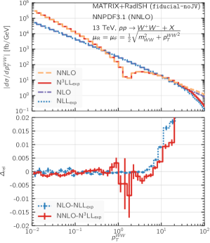
Figure 1: Left plot: transverse-momentum spectrum of the $W^{+}W^{-}$ pair at NLO (purple, dot-dashed) and NNLO (orange, dashed), and the expansion of the NLL (blue, dotted) and N³LL (red, solid) cross section. The lower panel shows the relative difference eq. (22) between the fixed-order cross section and the expansion. Right plot: the upper panel shows the difference at the cumulative level between NLO and NLL expansion (blue, dotted), and between NNLO and N³LL expansion (red, solid). The lower panel shows the same results for the derivative of the cumulative cross section with respect to $\ln(p_{T}^{WW}/{\rm GeV})$.

Thus, in order to perform a non-trivial check on the validity of our calculation we consider $W^{+}W^{-}$ production and study the small-$p_{T}^{WW}$ behaviour of the differential $p_{T}^{WW}$ distribution in the left plot of figure 1, where $p_{T}^{WW}$ is the transverse momentum of the $W^{+}W^{-}$ pair. In the upper (lower) panel of the right plot of figure 1 we show the corresponding cumulative (differential) cross section as a function of $\ln(p_{T}^{WW}/{\rm GeV})$. These results are obtained with the settings described in section 3.2.1 in the fiducial phase space defined as “fiducial-noJV”. By using dedicated high-statistics runs we were able to push the comparison down to remarkably low values of $p_{T}^{WW}=0.05$ GeV with statistical uncertainties below the permille level. The right plot of figure 1 indicates an excellent agreement for the $p_{T}^{WW}$ distribution between the fixed-order prediction and the respective logarithmic terms both at NLO and at NNLO. The dip around 1-2 GeV is due to the fact that the NNLO spectrum and the NNLL expansion become negative. In particular the relative difference

$$\Delta_{\rm rel}\equiv\left(\frac{{\rm d}\sigma^{\rm(N)NLO}}{{\rm d}p_{T}^{WW}}-\left[\frac{{\rm d}\sigma^{\rm(N)NLL}}{{\rm d}p_{T}^{WW}}\right]_{\rm(N)NLO}\right)\Bigg{/}\left[\frac{{\rm d}\sigma^{\rm(N)NLL}}{{\rm d}p_{T}^{WW}}\right]_{\rm(N)NLO}$$ (22)

in the lower panel shows the striking cancellation between those terms at the few-permille level for very small $p_{T}^{WW}$. At the cumulative level, on the other hand, the upper frame of the right plot of figure 1 nicely confirms that the NLO$-$NNLL_exp and the NNLO$-$N³LL_exp differences tend to zero, which validates our implementation of the constant terms at $\mathcal{O}(\alpha_{s})$ and $\mathcal{O}(\alpha_{s}^{2})$, respectively. Finally, in the lower panel of that figure we show the absolute differences of the differential distributions by taking the derivatives with respect to $\ln{p_{T}^{WW}}$. Although the information might appear slightly redundant, by considering the absolute difference here we unambiguously prove that there are no potential residual differences also for the subleading logarithmic contributions.

We have performed similar checks for other $2\to 1$ and $2\to 2$ colour-singlet processes, with various choices of the renormalisation scale $\mu_{R}$, the factorisation scale $\mu_{F}$, and the resummation scale $Q$. In particular, we performed the exact same study for fully inclusive $W^{+}W^{-}$ production, i.e. without fiducial cuts. In all cases we found an excellent agreement between the expansion of the resummed cross section and the fixed order result.

3 Resummed predictions for $W^{+}W^{-}$ production at the LHC

As a first application of the Matrix+RadISH framework introduced in section 2 we consider $W^{+}W^{-}$ production at the LHC. This process plays a prominent role in the vast physics programme at the LHC since it has the largest cross section among all diboson production processes. Experimental measurements of the $W^{+}W^{-}$ cross section at the Tevatron Aaltonen:2009aa ; Abazov:2011cb and at the LHC ATLAS:2012mec ; Chatrchyan:2013yaa ; ATLAS:2014xea ; Aad:2016wpd ; Chatrchyan:2013oev ; Khachatryan:2015sga ; Aaboud:2017qkn ; CMS:2016vww ; Aaboud:2019nkz provide crucial tests of the EW gauge sector of the SM and of the mechanism of EW symmetry breaking. Moreover, the production of $W$-boson pairs is an important probe of BSM physics. Since the dynamics of $W^{+}W^{-}$ production is sensitive to the value of the trilinear gauge coupling already at the Born level, $W^{+}W^{-}$ measurements put stringent bounds on the strength of anomalous trilinear gauge couplings in indirect searches for new physics ATLAS:2012mec ; Chatrchyan:2013yaa ; Khachatryan:2015sga ; Aad:2016wpd . $W^{+}W^{-}$ production contributes also as irreducible background to direct searches for BSM particles decaying into leptons, missing energy and/or jets, and to Higgs boson measurements in the $H\rightarrow W^{+}W^{-}$ decay channel. Since the two neutrinos prevent the reconstruction of the full event kinematics, an accurate theoretical description of the $W^{+}W^{-}$ final state is essential to enhance the experimental sensitivity in BSM searches and Higgs boson measurements.

Moreover, $W^{+}W^{-}$ analyses generally apply a rather stringent cut on the jet activity in order to deplete the signal contamination due to top-quark backgrounds. Such a jet veto introduces large logarithmic contributions in the calculation of the fiducial cross section, which challenges the validity of fixed-order predictions and induces an additional uncertainty in the extrapolation to the inclusive $W^{+}W^{-}$ cross section.

As a consequence, $W^{+}W^{-}$ production has received much attention in the past years in a joint effort to reduce theoretical uncertainties in order to match the increasing precision of the experimental data. Next-to-leading order (NLO) QCD Ohnemus:1991kk ; Frixione:1993yp predictions for on-shell $W$ bosons have been known for years, and leptonic $W$ boson decays were included in refs. Campbell:1999ah ; Dixon:1999di ; Dixon:1998py ; Campbell:2011bn . Due to large $\mathcal{O}(\alpha_{s})$ corrections, a substantial effort has been put into calculating contributions at $\mathcal{O}(\alpha_{s}^{2})$. The simplest $\mathcal{O}(\alpha_{s}^{2})$ correction is the loop-induced $gg\rightarrow W^{+}W^{-}$ subprocess, which is enhanced by the gluon luminosities. Leading order (LO) predictions for the loop-induced gluon fusion channel were studied in refs. Dicus:1987dj ; Glover:1988fe ; Binoth:2005ua ; Binoth:2006mf ; Campbell:2011bn ; Campbell:2011cu . The full NNLO QCD corrections were calculated first for the inclusive $W^{+}W^{-}$ cross section in the on-shell approximation in ref. Gehrmann:2014fva , and were later advanced to the fully differential level including leptonic decays in ref. Grazzini:2016ctr . Contrary to the common lore, the quark-initiated contributions were found to be the dominant NNLO QCD corrections at the inclusive level, with the loop-induced $gg$-initiated channel contributing only $\sim 30\%$ of the full $\mathcal{O}(\alpha_{s}^{2})$ correction. Various efforts have been made to go beyond NNLO QCD accuracy: NLO EW corrections were calculated for stable $W$ bosons Bierweiler:2012kw ; Baglio:2013toa ; Billoni:2013aba , and with a consistent treatment of the leptonic decays Biedermann:2016guo ; Kallweit:2019zez . The presumably dominant $\mathcal{O}(\alpha_{s}^{3})$ corrections are known from the calculation of the loop-induced gluon fusion contribution at NLO QCD Caola:2015rqy ; Caola:2016trd ; Grazzini:2020stb . The first combination of NNLO QCD predictions with NLO EW corrections was presented very recently in ref. Kallweit:2019zez , and ref. Grazzini:2020stb performed their further combination with NLO QCD corrections to the loop-induced $gg$ channel, yielding the best fixed-order prediction for the $W^{+}W^{-}$ process to date.

Analytic resummation approaches for different observables have been subject to various studies of $W^{+}W^{-}$ production. The transverse-momentum spectrum of on-shell $W^{+}W^{-}$ pairs was calculated at NNLO+NNLL accuracy in ref. Grazzini:2015wpa , and the resummation of jet veto logarithms at NNLO+NNLL accuracy was performed in ref. Dawson:2016ysj . In particular, the proper modelling of jet-vetoed $W^{+}W^{-}$ cross sections has attracted much attention in the theory community Jaiswal:2014yba ; Becher:2014aya ; Monni:2014zra ; Dawson:2016ysj , which has shown that higher-order corrections in both the perturbative and the logarithmic expansion are crucial to obtain reliable predictions and uncertainty estimates in presence of a jet veto cut in the fiducial phase space.

3.1 Outline of the calculation

We consider the process

$$pp\to\ell^{+}\ell^{\prime\,-}\nu_{\ell}{\bar{\nu}}_{\ell^{\prime}}+X,$$ (23)

where the charged final-state leptons and the corresponding (anti-)neutrinos have different flavours ($\ell\neq\ell^{\prime}$). All resonant and non-resonant contributions to this process are accounted for, including off-shell effects and spin correlations, employing the complex-mass scheme Denner:2005fg without any resonance approximation. We have full control on the momenta of the final-state leptons, which allows us to evaluate resummed cross sections in presence of fiducial selection criteria as employed by the experiments. Our calculation applies to an arbitrary combination of (massless) leptonic flavours, $\ell,\ell^{\prime}\in\{e,\mu\}$, and in order to compare against experimental data, we evaluate the process $pp\to\ell^{+}\ell^{\prime-}\nu_{\ell}{\bar{\nu}}_{\ell^{\prime}}+X$ with $\ell,\ell^{\prime}=e$ or $\mu$ and $\ell\neq\ell^{\prime}$. For the sake of simplicity, this process will be denoted as $W^{+}W^{-}$ production in the following.

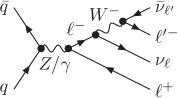
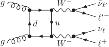
(a)	(b)	(c)	(d)

Figure 2: Feynman diagrams for $W^{+}W^{-}$ production: (a-c) sample tree-level diagrams in the quark-annihilation channel contributing at LO; (d) sample loop-induced diagram in the gluon fusion channel contributing at the NNLO.

In figure 2 (a–c) we show representative Feynman diagrams at LO for $W^{+}W^{-}$ production. They are driven by quark annihilation in the initial state and include $t$-channel $W^{+}W^{-}$ topologies (panel a), $s$-channel $W^{+}W^{-}$ topologies (panel b), and $s$-channel Drell–Yan-type topologies (panel c). Figure 2 (d), on the other hand, shows a loop-induced diagram that is driven by gluons in the initial state, which enters the cross section at ${\cal O}(\alpha_{s}^{2})$ and is part of the NNLO corrections. In an NNLO calculation the loop-induced gluon fusion contribution is, however, effectively only LO accurate and has Born kinematics. Without associated QCD radiation at fixed order, it contributes trivially to the differential observables we are considering in this paper. At the resummed level, the LL resummation of this contribution starts at $\mathcal{O}(\alpha_{s}^{3}L^{2})$, and it is thus of the same size as N³LL corrections to the $q\bar{q}$ channel. In principle the resummation of the loop-induced $gg$ channel can be included alongside the resummation of the $q\bar{q}$ channel. However, in terms of their respective resummation both contributions can be treated completely independently, and we refrain from considering the loop-induced gluon fusion contribution in what follows, since we reckon that its proper treatment requires to go beyond an effective accuracy of LO+LL. In fact, NLO QCD corrections to the loop-induced gluon fusion contribution have already been evaluated within the Matrix framework for both $ZZ$ Grazzini:2018owa and $W^{+}W^{-}$ Grazzini:2020stb production. They are strongly enhanced by the large gluon luminosity, and contributing at ${\cal O}(\alpha_{s}^{3})$ they constitute the dominant N³LO corrections to the cross sections of these two processes. These corrections involve diagrams with real QCD radiation that would directly contribute to the resummed observables under consideration. Therefore, a matching of the NLO QCD cross section with NNLL resummation for the loop-induced gluon fusion contribution would be a useful addition to the predictions presented below, which could be achieved within Matrix+RadISH, but it is beyond the scope of the present paper and left for future studies.

The calculation of higher-order corrections to the $W^{+}W^{-}$ production process in QCD perturbation theory is affected by a subtle interplay with contributions stemming from the production of off-shell top quarks, which mix through $t\rightarrow Wb$ decays Dittmaier:2007th ; Cascioli:2013gfa ; Gehrmann:2014fva ; Grazzini:2016ctr with real-radiation diagrams involving final-state bottom quarks. Due to the large cross section of top-quark processes at the LHC, these contributions induce a sizeable contamination of the $W^{+}W^{-}$ cross section. In order to deal with this problem, we employ the four-flavour scheme (4FS), where bottom quarks are treated as massive and do not appear as initial-state particles. The bottom-quark mass renders partonic subprocesses with bottom quarks in the final state separately finite. We then evaluate top-free $W^{+}W^{-}$ cross sections by omitting all subprocesses with real bottom-quark emissions, which in turn are considered to be part of the (off-shell) top-pair background. An alternative definition of the top-free $W^{+}W^{-}$ cross section can be obtained in the five-flavour scheme (5FS), where bottom quarks are treated as massless, by exploiting the scaling behaviour of the cross section with the top-quark width, which has been explained in detail in refs. Gehrmann:2014fva ; Grazzini:2016ctr . As it has been shown there, the top-free $W^{+}W^{-}$ cross sections resulting from the 4FS and 5FS prescriptions agree within $1\%-2\%$, both at the inclusive level and with fiducial cuts. Consequently, we exploit the simpler 4FS prescription throughout this paper. We note that this approach requires the use of consistent sets of parton distribution functions (PDFs) with $n_{f}=4$ light parton flavours.

We recall that our implementation allows us to obtain resummed predictions for different transverse observables in $W^{+}W^{-}$ production at the LHC. We calculate the transverse-momentum spectrum of $W^{+}W^{-}$ pairs at NNLO+N³LL accuracy as well as the transverse-momentum spectrum of the leading jet (and equivalently the jet-vetoed cross section) at NNLO+NNLL accuracy. Even more notably, we also perform the simultaneous resummation of both observables at the double-differential level at NNLO+NNLL accuracy, which allows us to evaluate the spectrum of one of the two observables in presence of a veto on the other one. For all differential observables presented here it is the first time that such accuracies are achieved for a nontrivial process, i.e. beyond $2\to 1$ scattering like Higgs boson production or the Drell–Yan process. In addition, arbitrary fiducial selection criteria can be applied in phase space of the leptonic final states.

3.2 Phenomenological results

3.2.1 Setup

We present resummed predictions for various observables in $pp\to\ell^{+}\ell^{\prime-}\nu_{\ell}{\bar{\nu}}_{\ell^{\prime}}+X$ production with $\ell,\ell^{\prime}=e$ or $\mu$ and $\ell\neq\ell^{\prime}$ at the LHC with $\sqrt{s}=13$ TeV. We employ the the $G_{\mu}$ scheme to evaluate the EW coupling $\alpha=\sqrt{2}\,G_{F}m_{W}^{2}\left(1-m_{W}^{2}/m_{Z}^{2}\right)/\pi$ and the mixing angle $\cos\theta_{W}^{2}=(m_{W}^{2}-i\Gamma_{W}\,m_{W})/(m_{Z}^{2}-i\Gamma_{Z}\,m_{Z})$, using the complex-mass scheme Denner:2005fg throughout. As input parameters we choose the PDG Patrignani:2016xqp values: $G_{F}=1.16639\times 10^{-5}$ GeV^-2, $m_{W}=80.385$ GeV, $\Gamma_{W}=2.0854$ GeV, $m_{Z}=91.1876$ GeV, $\Gamma_{Z}=2.4952$ GeV, $m_{H}=125$ GeV, and $\Gamma_{H}=0.00407$ GeV. The on-shell masses of bottom and top quarks are $m_{b}=4.92$ GeV and $m_{t}=173.2$ GeV, respectively, and the top width is set to $\Gamma_{t}=1.44262$ GeV. As discussed in the previous section, all predictions are calculated in the 4FS with $n_{f}=4$ massless quark flavours and massive bottom and top quarks, and all contributions with real bottom quarks in the final state are dropped to avoid the contamination from top-quark production processes. Accordingly, we use the $n_{f}=4$ NLO and NNLO sets of the NNPDF3.1 PDFs at NLO(+NLL) and at NNLO(+NNLL/N³LL) Ball:2017nwa , respectively, by exploiting the Lhapdf interface Buckley:2014ana with the corresponding values of the strong coupling. Jets are defined according to the anti-$k_{t}$ algorithm Cacciari:2008gp with a jet radius of $R=0.4$ and no rapidity requirements.

lepton cuts	$p_{T,{\ell}}>27$ GeV,  $|\eta_{\ell}|<2.5$,  $m_{\ell^{-}\ell^{+}}>55$ GeV,  $p_{T,\rm\ell^{-}\ell^{+}}>30$ GeV
neutrino cuts	$p_{T}^{\text{miss}}>20$ GeV
jet cuts	anti-$k_{T}$ jets with $R=0.4$;
	$N_{\rm jet}=0$ for $p_{T}^{J}>35$ GeV
	(our results do not include any cut on $\eta_{\rm jet}$, see text)

Table 1: Fiducial cuts corresponding to the 13 TeV ATLAS analysis Aaboud:2019nkz . See text for details.

We employ the following dynamical setting for the central factorisation and renormalisation scales,

$$\mu_{F}=\mu_{R}=\mu_{0}=\frac{1}{2}\sqrt{M_{WW}^{2}+{p_{T}^{WW}}^{2}},$$ (24)

and set the central resummation scale to

$$Q=Q_{0}=\frac{1}{4}M_{WW},$$ (25)

where $M_{WW}$ is the invariant mass of the $W^{+}W^{-}$ pair and $p_{T}^{WW}$ is its transverse momentum. Perturbative uncertainties are estimated by performing seven-point scale variations of $\mu_{F}$ and $\mu_{R}$ around $\mu_{0}$ by a factor of two in either direction, keeping $1/2\leq\mu_{F}/\mu_{R}\leq 2$ for $Q=Q_{0}$, and by varying $Q$ by a factor of two around $Q_{0}$ in either direction for $\mu_{F}=\mu_{R}=\mu_{0}$. The total scale uncertainty is evaluated as the envelope of the resulting nine variations. For the exponent of the modified logarithm in eq (15) we choose a value of $p=4$ when evaluating the resummed $p_{T}^{WW}$ spectra and $p=5$ for the jet-vetoed cross section as well as the $p_{T}^{J}$ distribution. We have explicilty checked that the dependence of the results on variations of $p$ is negligible. Moreover, no non-perturbative corrections are included in our results.

In table 1 we summarise the set of fiducial cuts used in our study. Those cuts are the same as in the fiducial selection of the 13 TeV analysis of ATLAS in ref. Aaboud:2019nkz , with the only exception that we do not apply any rapidity requirement on the jets since this would generate logarithmic corrections of non-global nature, which would spoil the formal accuracy of our resummed results. Furthermore, we introduce two notations: fiducial-JV will be used to refer to the full set of fiducial cuts in table 1, while fiducial-noJV denotes the same fiducial setup, but without any restriction on the jet activity.

3.2.2 Jet-vetoed cross section

We consider the cumulative cross section in the fiducial phase space as a function of a veto on the transverse momentum of the leading jet (${p_{T}^{J,{\rm veto}}}$) as generically defined in eq. (2) where we identify the upper bound of the integral with the jet-veto cut ${p_{T}^{J,{\rm veto}}}$, i.e.

$$\sigma({p_{T}^{J,{\rm veto}}})=\int_{0}^{p_{T}^{J,{\rm veto}}}\mathrm{d}p_{T}^{J}\,\frac{\mathrm{d}\sigma}{\mathrm{d}p_{T}^{J}}\,.$$ (26)

The corresponding jet-veto efficiency is defined as

$$\varepsilon({p_{T}^{J,{\rm veto}}})=\sigma({p_{T}^{J,{\rm veto}}})/\sigma({p_{T}^{J,{\rm veto}}}\rightarrow\infty)\,,$$ (27)

where $\sigma({p_{T}^{J,{\rm veto}}}\rightarrow\infty)$ is the integrated cross section in the fiducial-noJV phase space.

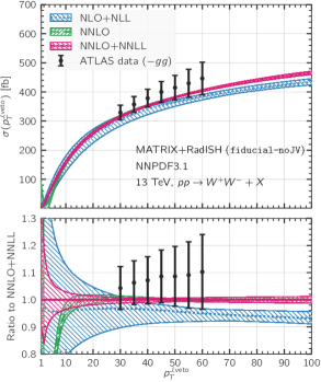
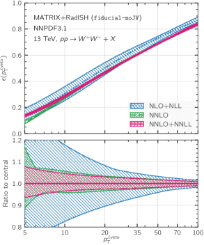
Figure 3: Fiducial cross sections (left plot) and jet-veto efficiencies (right plot) as a function of the jet-veto cut at NLO+NLL (blue, dotted), NNLO (green, dashed), and NNLO+NNLL (red, solid). In the left plot, we also show the fiducial cross sections measured by ATLAS Aaboud:2019nkz , from which we have subtracted the loop-induced gluon fusion contribution at LO that simply amounts to a constant shift independent of ${p_{T}^{J,{\rm veto}}}$ (see text for details).

In figure 3 we show results for the jet-vetoed cross section and the jet-veto efficiency as a function of ${p_{T}^{J,{\rm veto}}}$. In the case of the cumulative cross section, we compare our predictions with the cross-section measurements from the ATLAS experiment at $13$ TeV Aaboud:2019nkz . Since our resummed predictions do not include the loop-induced gluon fusion contribution, we have subtracted its LO prediction from the experimental results to facilitate a meaningful comparison. We observe that the NNLO result is in remarkable agreement with the NNLO+NNLL prediction down to jet-veto cuts of ${p_{T}^{J,{\rm veto}}}\gtrsim 15$ GeV. Below $\sim 10$ GeV the fixed-order result becomes unphysical, and the central prediction eventually turns negative. The fixed-order scale uncertainty band vastly underestimates missing higher-order corrections since this region is dominated by large logarithms. The uncertainties of the resummed results increase below $10$ GeV, and by comparing NNLO+NNLL and NLO+NLL results it is clear that higher-order corrections in both the fixed-order and the logarithmic expansion are substantial and mandatory to provide reliable scale uncertainties, reduced to the few-percent level. Due to the relatively large experimental uncertainties, all predictions are in reasonably good agreement with the data. To better appreciate resummation effects in the comparison with data, it would be required to push the measurements to much lower jet-veto cuts.

Looking at the jet-veto efficiency in the right plot of figure 3, at $35$ GeV, which is the value of the jet veto used in the fiducial phase space definition, the efficiency is $65$%, and agreement between the NNLO and the NNLO+NNLL results is at the few permille level. Scale uncertainties for the efficiencies are calculated by considering fully correlated scale variations between the numerator and denominator of eq. (27). The scale uncertainty at NNLO+NNLL is about $5$% at $p_{T}\sim 5$ GeV, and it decreases towards larger values of the jet veto, being about $2$% at $p_{T}\sim 35$ GeV. The inclusion of the higher-order corrections reduces significantly the perturbative uncertainties, as illustrated by the NLO+NLL and the NNLO+NNLL bands.

3.2.3 Differential distributions

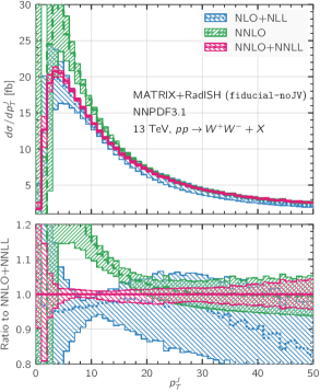
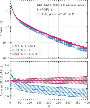
Figure 4: Transverse-momentum spectrum of the leading jet in the fiducial-noJV phase space at NLO+NLL (blue, dotted), NNLO (green, dashed), and NNLO+NNLL (magenta, solid) accuracy. Left plot: spectrum up to 50 GeV. Right plot: spectrum up to 200 GeV. The lower frames show the ratios of the predictions to the central value of our best prediction at NNLO+NNLL.

We now move to differential results in the fiducial-noJV phase space. In figure 4 we show the transverse-momentum spectrum of the leading jet. The central value of the NNLO+NNLL prediction lies within the uncertainty band of the NLO+NLL result for $p_{T}^{J}\lesssim 50$ GeV. At larger $p_{T}^{J}$, where the (N)NLO+(N)NLL result matches the (N)NLO one, the uncertainty bands do not overlap anymore with a visible gap between them in the tail of the distribution. This indicates that NNLO corrections are particularly important at high values of $p_{T}^{J}$. Resummation effects become crucial for $p_{T}^{J}\lesssim 20$ GeV, where the NNLO distribution is marred by large logarithmic contributions and starts diverging. The NNLO+NNLL curve is instead well-behaved, and it has perturbative uncertainties of only a few percent down to $p_{T}^{J}\sim 5$ GeV. Below that value, the uncertainty band becomes wider, reaching up to $20\%$ in the first two bins. We note, however, that these regions are likely beyond experimental reach. In the tail of the NNLO+NNLL prediction the uncertainties gradually increase from about $5\%$ at $p_{T}^{J}=50$ GeV to about $10\%$ at $p_{T}^{J}=400$ GeV. The Sudakov peak of the resummed $p_{T}^{J}$ spectrum is around $4$–$5$ GeV both at NLO+NLL and at NNLO+NNLL.

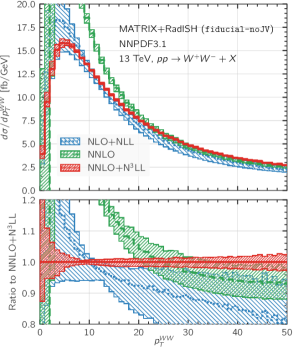
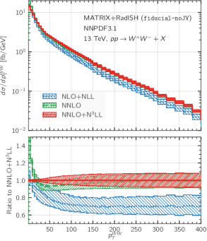
Figure 5: Transverse-momentum spectrum of the $W^{+}W^{-}$ pair in the fiducial-noJV phase space at NLO+NLL (blue, dotted), NNLO (green, dashed), and NNLO+N³LL (red, solid) accuracy. Left plot: spectrum up to 50 GeV. Right plot: spectrum up to 200 GeV. The lower frames show the ratios of the predictions to the central value of our best prediction at NNLO+N³LL.

In figure 5 we show the transverse-momentum spectrum of the $W^{+}W^{-}$ pair at NNLO as well as matched predictions at NLO+NLL and at NNLO+N³LL. For $p_{T}^{WW}\lesssim 20$ GeV, the NNLO result starts diverging and thus loses predictivity. In that region only the matched results are well-behaved since the resummation of large logarithmic contributions becomes indispensable to obtain a physical prediction. The peak of the NNLO+N³LL spectrum is around $5$–$6$ GeV, and it is shifted with respect to the NLO+NLL prediction by about $1$ GeV, which peaks around $4$–$5$ GeV. Also at larger values of $p_{T}^{WW}$, roughly up to $2\,m_{W}$, the NNLO and NNLO+N³LL curves differ by about $1$%–$6$%, which indicates that in this intermediate region there are important effects due to the interplay between the resummation of large logarithmic contributions and the matching. The matched result at NNLO+N³LL features very small uncertainties, which are at the few-percent level below $50$ GeV and gradually increase in the peak region and below ($p_{T}^{WW}\lesssim 8$ GeV), where the logarithmic terms are dominant. We note that, since the scale variation band is so small, it does not necessarily capture the actual size of the uncertainties due to missing higher-order terms. For $20\lesssim p_{T}^{WW}\lesssim 50$ GeV the scale uncertainties of the matched NNLO+N³LL prediction are only $2$%–$3$%, and more than a factor of 2 smaller than those of the NNLO result. In this region, the uncertainty bands at NNLO and NNLO+N³LL overlap only marginally. The importance of higher-order corrections in the fixed-order expansion manifests itself especially in the tail of the distribution, where the NNLO result is about $30\%$ larger than the NLO+NLL one.

To further study resummation effects in the region $p_{T}^{WW}\lesssim 50$ GeV, we compare the result at NNLO+N³LL to the one at NNLO+NNLL in the left plot of figure 6. The effect of the N³LL corrections on the central prediction is quite sizeable, especially below $10$ GeV, where it reaches almost $10$%. The uncertainty bands, however, largely overlap, with the central prediction at NNLO+N³LL being fully contained within the NNLO+NNLL band. The inclusion of NNLO+N³LL corrections reduces the scale uncertainties by a bit less than a factor of two.

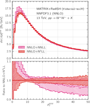
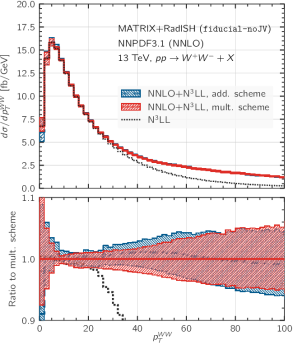
Figure 6: Left plot: transverse-momentum spectrum of the $W^{+}W^{-}$ pair in the fiducial-noJV phase space comparing predictions at NNLO+NNLL (magenta, dotted) and NNLO+N³LL (red, solid) accuracy. The lower frame shows the ratios of the predictions to the central value of the NNLO+N³LL result. Right plot: same distribution comparing additive (dark blue, dashed) and multiplicative (red, solid) matching schemes at NNLO+N³LL. The lower frame shows the ratios of the predictions to the central value of the multiplicative result.

To illustrate uncertainties due to higher-order effects of the NNLO+N³LL prediction in the small-$p_{T}^{WW}$ region, we compare the results for two different matching schemes, defined in eqs. (18) and (19), in the right plot of figure 6. At this accuracy, the two predictions contain the same ingredients and are compared on equal footing. We observe an excellent agreement between the two prescriptions, which indicates that our predictions exhibit a very mild dependence on the choice of the matching scheme. Only at very small transverse momenta ($p_{T}^{WW}\lesssim 2$ GeV) we observe minor differences between the multiplicative result and the additive result due to the higher sensitivity of the additive matching to the exact cancellation between the fixed-order cross section and the expansion. The advantage of the multiplicative scheme is confirmed by the fact that the multiplicative matching is in perfect agreement with the pure N³LL result, as it should be at very small transverse momenta, whereas the additive result is slightly different. Since the cancellation in the additive matching prescription is numerically challenging in this region, dedicated runs as those performed in section 2.4 would be required to achieve a more stable result.

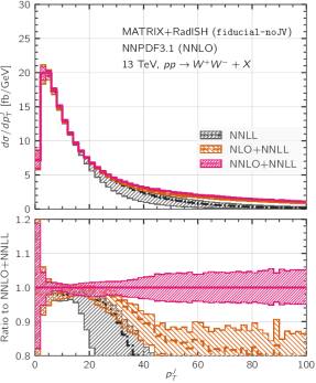
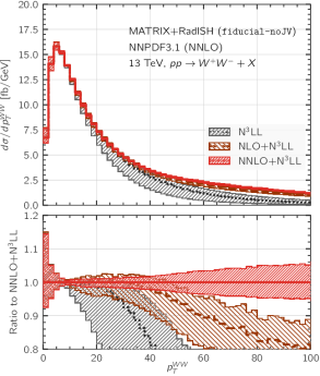
Figure 7: Left plot: transverse-momentum spectrum of the leading jet in the fiducial-noJV phase space comparing predictions at NNLO+NNLL (magenta, solid), NLO+NNLL (ochre, dashed) and NNLL (black, dot-dashed) accuracy. The lower frame shows the ratios of the predictions to the central value of the NNLO+NNLL result. Right plot: transverse-momentum spectrum of the $W^{+}W^{-}$ pair in the fiducial-noJV phase space comparing predictions at NNLO+N³LL (red, solid), NLO+N³LL (brown, dashed) and N³LL (black, dotted) accuracy (right plot). The lower frame shows the ratios of the predictions to the central value of the NNLO+N³LL result.

So far we have demonstrated the importance of resummation at small transverse momentum and of NNLO corrections in the tail of the $p_{T}^{J}$ and $p_{T}^{WW}$ spectra. However, the plots in figure 4 and figure 5 are not sufficient to appreciate the impact of the matching to NNLO at small and intermediate values of $p_{T}^{J}$ and $p_{T}^{WW}$. To this end, in the left (right) plot of figure 7 we investigate the impact of the NNLO corrections in the peak and in the matching region by comparing NNLL (N³LL) and NLO+NNLL (NLO+N³LL) predictions to our NNLO+NNLL (NNLO+N³LL) results for $p_{T}^{J}$ ($p_{T}^{WW}$). Below $\sim 20$ GeV matching effects play a minor role, while beyond this value the non-singular corrections become large and the purely resummed result unreliable. Note that for $p_{T}^{J}\lesssim 20$ GeV there is a moderate increase of $\sim 2\%$ originating from the inclusion of NNLO corrections in the matching. This difference can be traced back to the the NNLO constant terms in $p_{T}^{J}$, which are absent in the NNLL result and are included through the multiplicative matching at small $p_{T}^{J}$, as discussed in section 2.4. That behaviour is not observed for $p_{T}^{WW}$, since the N³LL result already includes the NNLO constant terms. Looking at the matching region, the inclusion of NNLO corrections becomes important for $p_{T}^{J}\gtrsim 30$ GeV and $p_{T}^{WW}\gtrsim 40$ GeV. Already at $p_{T}^{J}\sim 35$ GeV and $p_{T}^{WW}\sim 50$ GeV the uncertainty bands of the predictions matched to NLO and to NNLO do not overlap anymore. Not least, the matching to NNLO has a substantial impact on the size of the uncertainty bands, which above $p_{T}^{J}\sim 25$ GeV and $p_{T}^{WW}\sim 10$ GeV are reduced by roughly a factor of two. In conclusion, NNLO accuracy plays an important role not only for the accurate description of the high-$p_{T}{}$ tail, but also in the matching region.

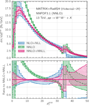
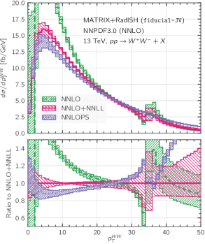
Figure 8: Left plot: transverse-momentum spectrum of the $W^{+}W^{-}$ pair with a jet-veto requirement in the fiducial-JV phase space at NLO+NLL (blue, dotted), NNLO (green, dashed), and NNLO+NNLL (red, solid) accuracy. Right plot: same distribution comparing NNLO (green, dashed) and NNLO+NNLL (red, solid) predictions to the NNLOPS result (blue, dotted) of ref. Re:2018vac . To facilitate the comparison, we reanalysed the NNLOPS events and we recalculated our predictions with the NNPDF3.0 NNLO PDF set Ball:2014uwa . The lower frame shows the ratios of the predictions to the central value of the NNLO+N³LL result.

We continue our studies by considering the transverse-momentum spectrum of the $W^{+}W^{-}$ system in presence of a jet veto. To this end, we perform the joint resummation of large logarithmic terms in both $p_{T}^{WW}$ and $p_{T}^{J}$. In the left plot of figure 8, we compare resummed predictions for the $p_{T}^{WW}$ spectrum in the fiducial-JV phase space at NLO+NLL and NNLO+NNLL accuracies to the NNLO result. By exploiting the multiplicative matching scheme at the double-differential level, defined in eq. (21), we include the constant terms in the resummed prediction, and the integral of the NLO+NLL (NNLO+NNLL) $p_{T}^{WW}$ spectrum yields the NLO+NLL (NNLO+NNLL) jet-vetoed cross section. The NNLO curve develops a perturbative instability Catani:1997xc right at $p_{T}^{WW}=35$ GeV, which corresponds to the value of the jet-veto cut. This instability is caused by an incomplete cancellation between soft contributions in the real and virtual amplitudes, and it leads to an integrable logarithmic divergence at the threshold. Since $p_{T}^{WW}=p_{T}^{J}$ holds at LO, and consequently $p_{T}^{WW}<35$ GeV, the $p_{T}^{WW}$ region above the jet-veto cut is filled only by higher-order corrections, and the effective perturbative accuracy is reduced by one order. This is indicated by the widening of the uncertainty band of the NNLO prediction for $p_{T}^{WW}>35$ GeV, which effectively becomes NLO accurate in that region.

The sensitivity to the perturbative instability at the threshold is largely cured by the NNLO+NNLL result, resumming a large part of the relevant logarithms. However, a slight sensitivity remains due to the fact that our approach resums Sudakov logarithms in the limit where $p_{T}^{WW}$ and $p_{T}^{J}$ are much smaller than the hard scale, while additional logarithmic terms contribute when hard jets are present. Nevertheless, the large differences between the NNLO+NNLL and NNLO results indicate the importance of resummation at the threshold. We observe even larger resummation effects for transverse momenta below $20$ GeV, where the NNLO result becomes unphysical and resummation is mandatory to retain a reliable prediction. The resummed spectra at NLO+NLL and NNLO+NNLL are consistent with each other at small $p_{T}^{WW}$, with fully overlapping uncertainty bands up to $p_{T}^{WW}\sim 30$ GeV.

The theoretical uncertainty of the NNLO+NNLL prediction is at the few-percent level in that region and roughly a factor of two smaller than the NLO+NLL uncertainty band. It reaches $\mathcal{O}(10\%)$ uncertainties only for $p_{T}^{WW}\lesssim 6$ GeV, where the logarithmic corrections become larger. When approaching the perturbative instability, the differences between NLO+NLL and NNLO+NNLL progressively increase, with barely overlapping uncertainties below the threshold. At the threshold theory uncertainties of the NNLO+NNLL result reach $30\%$. The large differences between the resummed results and the widening of the uncertainty bands further indicate that additional logarithmic terms contribute at the jet-veto threshold, which are not resummed. Beyond threshold the NLO+NLL result becomes unreliable, being effectively only LO accurate, while the NNLO+NNLL prediction is effectively NLO accurate with an enlarged uncertainty band at the $20$%–$30$% level.

In conclusion, our results indicate that the inclusion of higher-order corrections both in the fixed-order and the logarithmic expansion is particularly relevant for an accurate description of the $p_{T}^{WW}{}$ distribution in presence of a jet veto. To further study resummation effects for this observable, we compare the results at NNLO+NNLL with the NNLOPS results of ref. Re:2018vac in figure 8. By and large, the two results are in reasonable agreement. At very small $p_{T}^{WW}$ their uncertainty bands overlap. There is a gap between them for $5\,\text{GeV}\lesssim p_{T}^{WW}\lesssim 15$ GeV, because the NNLO+NNLL band almost vanishes at $p_{T}^{WW}\sim 10$ GeV, and thus underestimates the actual uncertainties in that region, and also the NNLOPS band, which misses uncertainties related to the shower-starting scale, is somewhat underestimated. For $p_{T}^{WW}\lesssim 25$ GeV, the NNLO+NNLL result provides the more accurate and therefore more reliable prediction. When approaching the threshold at $35$ GeV, the two results agree within uncertainties due to the rather large NNLO+NNLL band. The NNLOPS result is smooth in that region and develops no perturbative instability. At higher $p_{T}^{WW}$ values, the NNLOPS prediction becomes significantly larger than the NNLO+NNLL result since the shower generates additional QCD radiation, as discussed in ref. Re:2018vac . The comparison shows that in the low-$p_{T}^{WW}$ region high-accuracy resummation is required for a precise prediction of the spectrum. For values of $p_{T}^{WW}$ at and above the threshold, the NNLOPS result gives a more reliable description of the spectrum in the fiducial region, as it includes effects that are not included in other approaches, albeit with a limited formal accuracy.

4 Summary

In this paper we have introduced a general framework for the computation of accurate cross-section predictions including multi-differential resummation. By developing an interface between the codes Matrix and RadISH we have combined fully differential NNLO QCD predictions for $2\rightarrow 1$ and $2\rightarrow 2$ colour-singlet production processes with high-accuracy all-order resummation. In particular, Matrix+RadISH evaluates the transverse-momentum spectrum of colour singlets and the $\phi^{*}_{\eta}$ distribution for the Drell–Yan process up to NNLO+N³LL accuracy, the transverse-momentum spectrum of the leading jet and jet-veto resummation up to NNLO+NNLL accuracy, as well as the joint resummation of the colour-singlet and the leading-jet transverse momentum up to NNLO+NNLL. Thereby we provide a powerful and versatile parton-level Monte Carlo generator allowing for an accurate description of transverse observables in colour-singlet production processes with arbitrary cuts on the Born kinematics. This framework can be extended to describe any observable differential in the Born kinematics including resummation effects by exploiting a suitable scheme for the kinematic recoil within the resummation. Moreover, the framework facilitates the combination of future developments within Matrix and RadISH, such as advancements towards processes beyond colour-singlet production.

As a first phenomenological application we have studied the production of $W^{+}W^{-}$ pairs at the LHC. More precisely, the full leptonic final state of two charged different-flavour leptons and two neutrinos has been considered, including spin correlations, interferences and off-shell effects. We have presented resummed results at $13$ TeV for several kinematic distributions in presence of fiducial cuts on the leptonic final states and the associated QCD radiation. The inclusion of higher-order corrections in both the logarithmic and the fixed-order expansion turns out to be essential to achieve a precise description of differential observables at the few-percent level, as demanded by the experimental analyses. The accurate modelling of the cross section in presence of a veto against hard QCD radiation is particularly important in that respect since a jet veto is commonly employed in $W^{+}W^{-}$ measurements to suppress top-quark backgrounds. Our NNLO+NNLL result yields residual uncertainties at the few-percent level, we have shown that NNLO predictions are reliable down to jet-veto cuts of roughly $15$ GeV, and we find agreement within one standard deviation with the cross section measured by ATLAS as a function of the jet-veto cut between $30$ GeV and $60$ GeV.

For the differential spectra in the transverse momentum of the leading jet and the $W^{+}W^{-}$ pair, which we have evaluated up to NNLO+NNLL and NNLO+N³LL accuracy, respectively, we obtain scale uncertainties that are generally below 5%. Furthermore, our results highlight the importance of high-accuracy resummation in the region of the Sudakov peak, and of the $\mathcal{O}(\alpha_{s}^{2})$ corrections in the tail of the distribution. Indeed, scale variations at $\mathcal{O}(\alpha_{s})$ significantly underestimate the actual size of $\mathcal{O}(\alpha_{s}^{2})$ corrections at large transverse momenta. At small transverse momenta, N³LL corrections to the $W^{+}W^{-}$ transverse-momentum distribution are still quite sizable, with differences of about 5% –10% when comparing NNLO+N³LL to NNLO+NNLL.

The matching of the resummed cross section, valid in the soft-collinear region, and the fixed-order predictions, valid in the hard region, can be achieved in different ways. We have shown that a multiplicative matching procedure, which at NNLL resums additional logarithmic contributions originating from the NNLO terms that are constant in the resummation variable, has the further advantage of being numerically more stable at small transverse momenta than the additive matching procedure. Furthermore, we found that at NNLO+N³LL there is essentially no dependence of the $W^{+}W^{-}$ transverse-momentum spectrum on the choice of the matching scheme.

Finally, we have studied the transverse-momentum distribution of $W^{+}W^{-}$ pairs in presence of a $35$ GeV jet-veto requirement by simultaneously resumming both classes of logarithmic terms. At fixed order no realistic description of this observable can be obtained. Resummed results at NLO+NLL and NNLO+NNLL indicate good perturbative convergence at small transverse momenta (below $\sim 30$ GeV), and the inclusion of the NNLO+NNLL corrections decreases scale uncertainties by roughly a factor of two in that regime. The most delicate region is the threshold where the $W^{+}W^{-}$ transverse momentum is close to the value of the jet-veto cut since this region is subject to a perturbative instability at fixed order in $\alpha_{s}$. The joint resummation of jet-veto logarithms and logarithmic terms in the $W^{+}W^{-}$ transverse momentum improves the stability of the spectrum in the threshold region by resumming part of the relevant logarithms. We have further compared our NNLO+NNLL results to NNLOPS predictions, which corroborates the importance of NNLL resummation for an accurate modeling at small transverse momenta. In the threshold region the NNLOPS result is smooth, and we found it to be in reasonable agreement with NNLO+NNLL predictions, well within the respective scale uncertainties.

In all presented results we refrained from including the loop-induced gluon fusion contribution, which is formally part of the NNLO corrections, because it is effectively only LO accurate and Born-like. Although at fixed order it contributes trivially to all observables we have considered, i.e. as a constant shift in the cross sections, at the resummed level it is of the same size as N³LL corrections to the quark channel. Since their resummation can be considered completely independently, we leave a proper treatment of the loop-induced gluon fusion contribution, and specifically the combination of its NLO corrections with NNLL resummation, for future work.

We reckon that the predictions presented in this paper for the specific case of $W^{+}W^{-}$ production as well as the Matrix+RadISH framework in general will be a very useful addition to current fixed-order and parton-shower predictions and tools. With this framework we hope to advance the sensitivity to transverse observables in colour-singlet processes for precision measurements and new-physics searches at the LHC and future $pp$ colliders.

Appendix A How to use Matrix+RadISH

The aim of this appendix is to provide some guidance on the usage of the Matrix+RadISH interface. Beside some additional parameters in the input files, mostly related to RadISH, and some necessary modifications to the structure of the output to accommodate the additional histograms, a Matrix+RadISH run is very similar to a fixed-order run in Matrix. Therefore, we shall describe only the main steps needed to produce resummed predictions and provide only basic information on Matrix here, while focussing on the aspects that are different in Matrix+RadISH. We refer the reader to ref. Grazzini:2017mhc for a comprehensive overview of all the settings available in Matrix and a complete description of the structure of the code. If the reader has never run a fixed-order computation with Matrix, we encourage them to consult the Matrix manual in ref. Grazzini:2017mhc , and in particular section 3 therein, before reading this appendix.

A.1 Compilation and setup of a process

We assume that the MATRIX+RadISH_v1.0.0.tar.gz package has been downloaded and extracted, and that a working installation of Lhapdf Buckley:2014ana is present on the machine such that the shell command lhapdf-config is recognised when it is run in a terminal. We also require a working Python 2.7 installation. If these requirement have been met, the command

commandchars=

{},,,

  \ExtensionTok{\$  ./matrix}\NormalTok{ --radish}

executed inside the MATRIX+RadISH_v1.0.0 folder will launch the Matrix shell with the RadISH interface enabled. An interactive Python session for the compilation will appear, with instructions printed on the screen. This is followed by the usual steps in the Matrix shell to select a process via its ${process_id}, e.g. for Drell–Yan production

commandchars=

{},,,

  \ExtensionTok{|===>> ppz01}

and to agree with the terms to use Matrix+RadISH by typing (a few times)

commandchars=

{},,,

  \ExtensionTok{|===>> y}

This requires you to acknowledge the work of various groups that went into the computation performed by Matrix+RadISH for the present process by citing the references collected in the file CITATION.bib, which is provided with the results in every run. The compilation shell will then execute the following steps:

• linking to Lhapdf Buckley:2014ana ;

• download and installation of OpenLoops Cascioli:2011va ; Buccioni:2017yxi ; Buccioni:2019sur (skipped if already installed);

• installation of CLN Haible:1998xxx (skipped if already installed);

• installation of GiNaC Bauer:2000cp (skipped if already installed);

• installation of Hoppet Salam:2008qg (skipped if already installed);

• installation of Chaplin Buehler:2011ev (skipped if already installed);

• installation of RadISH Monni:2016ktx ; Bizon:2017rah ; Monni:2019yyr (skipped if already installed);

• compilation of Matrix process (asked for recompilation if executable exists);

• download of the relevant tree-level and one-loop amplitudes through OpenLoops (skipped if they already exist);

• setting up of the process folder under the path run/${process_id}_MATRIX .

Once completed, the shell will exit and the process is ready to be run from the created process folder. As instructed on screen, enter that folder (cd run/${process_id}_MATRIX) and start a run by following the instructions in the next section.

A.2 Running a process in the interactive shell

Once the process has been compiled, we launch the running shell with the usual command

commandchars=

{},,,

\ExtensionTok{\$ ./bin/run_process}

inside the folder (cd run/${process_id}_MATRIX). With this interactive steering interface all run-related settings, inputs, and options will be handled just as in a standard Matrix run. After typing a name for the run, e.g.

commandchars=

{},,,

  \ExtensionTok{|===>> run_name_resummation}

a list of several commands is printed on the screen. Before starting the run, the only differences with respect to an ordinary Matrix run are the inputs of the files parameter.dat and distribution.dat of the current run inside the folder input. We open them by typing

commandchars=

{},,,

  \ExtensionTok{|===>> parameter}

  \ExtensionTok{|===>> distribution}

and we modify the settings to turn on the resummation as discussed in appendix A.4. Once the input cards have been adjusted to obtain the desired results, the run is started through the usual command:

commandchars=

{},,,

  \ExtensionTok{|===>> run }

From now on, no human intervention is needed. Once the run is finished, the results from the run are collected in the respective folder result/${run_name_resummation}, which is printed on screen at the end of the run.

The only difference, compared to an ordinary fixed-order Matrix run, after a run with resummation has been completed, is that there will be additional results inside the folder result/${run_name_resummation}. In particular, there will be the following information:

• The same results as in a fixed-order run are saved, and the general structure is identical.

• If resummation for the respective orders has been turned on in the file parameter.dat, as discussed in appendix A.4.1, inside the folders NLO-run and NNLO-run a folder MATRIX+RadISH is present.

• The folder MATRIX+RadISH contains the resummed differential distributions (ending with NLL.dat, NNLL.dat or N3LL.dat), the corresponding fixed-order differential distributions (ending with NLO_QCD.dat or NNLO_QCD.dat), the matched distributions at differential level (ending with NLO+NLL.dat, NNLO+NNLL.dat or NNLO+N3LL.dat), which correspond to the best and final prediction, and, for completeness, the expansion of the resummed cross section at the relevant order (ending with exp_NLO_QCD.dat or exp_NNLO_QCD.dat).

• There is a further subfolder cumulant inside MATRIX+RadISH that contains the respective cumulative cross sections obtained from the differential distributions.

A.3 Additional settings in the configuration file

variable	description
path_to_radish	Path to the RadISH installation; not required in most cases.
path_to_hoppet	Path to hoppet-config; not required in most cases.
path_to_chaplin	Path to the Chaplin installation; not required in most cases.

Table 2: Additional parameters available the file MATRIX_configuration.

Before turning to physics-related and technical settings relevant for a Matrix+RadISH run in the next section, the additional parameters in the file MATRIX_configuration are discussed. The main file MATRIX_configuration can be found in the folder config inside the Matrix+RadISH main folder. This file is linked during each setup of a process (see appendix A.1) into the folder input of the respective process folder. The additional options for a Matrix+RadISH run in the file MATRIX_configuration are listed in table 2.

A.4 Additional settings in parameter.dat and distribution.dat

The various parameters in the input files are described in section 4.1 of ref. Grazzini:2017mhc . Here we will discuss only the additional settings in the files parameter.dat and distribution.dat that are relevant when performing a run in Matrix+RadISH.

A.4.1 Settings in parameter.dat

All main parameters, related to the run itself or the behaviour of the code, are specified in the file parameter.dat. Most of them should be completely self-explanatory, and we will focus our discussion on the essential ones with a direct connection to the resummation. The settings are organized into certain groups. Here, we will limit the discussion to the groups which contain additional information when the Matrix+RadISH interface is enabled, for the sample case of $Z\gamma$ production (where applicable) as in ref. Grazzini:2017mhc .

A.4.1.1   Scale settings

⬇

scale_ren = 91.1876 # renormalization (muR) scale

scale_fact = 91.1876 # factorization (muF) scale

dynamic_scale = 6 # dynamic ren./fac. scale (not working with resummation)

# 0: fixed scale above

# 1: invariant mass (Q) of system (of the colourless final states)

# 2: transverse mass (mT^2=Q^2+pT^2) of system (of the colourless final states)

# 3: transverse mass of photon (note: mT_photon=pT_photon)

# 4: transverse mass of Z boson (lepton system, mT_lep1+lep2)

# 5: geometric avarage of mT of photon and mT of Z boson

# 6: quadratic sum of Z mass and mT of the photon (mu^2=m_Z^2+mT_photon^2)

# 7: quadratic sum of dilepton mass and mT of photon (mu^2=m_lep1+lep2^2+mT_photon^2)

factor_central_scale = 1 # relative factor for central scale (important for dynamic scales)

scale_variation = 1 # switch for muR/muF uncertainties (0) off; (1) 7-point (default); (2) 9-point variation

variation_factor = 2 # symmetric variation factor; usually a factor of 2 up and down (default)

# scale settings for resummation

scale_res = 91.1876 # resummation scale

dynamic_scale_res = 1 # dynamic resummation scale

# 0: fixed scale above

# 1: invariant mass (Q) of system (of the colourless final states)

factor_scale_res = 0.5 # relative factor for central resummation scale (important for dynamic scale)

scale_variation_res = 1 # switch for resummation-scale uncertainties (0) off; (1) on (default);

variation_factor_res = 2 # symmetric variation factor; usually a factor of 2 up and down (default)

dynamic_scale This parameter is present already in a fixed-order run to choose between the specified fixed renormalisation and factorisation scales (scale_ren/scale_fact) and dynamic ones, and we refer the reader to the information given section 5.1.1.2 of ref. Grazzini:2017mhc for details. In a resummed calculation it is important to only use sensible choices for dynamical scales, i.e. any choice that depends on QCD radiation must smoothly approach the scale at Born level in the limit where the QCD radiation becomes soft or collinear. In particular, this allows for any dynamical scale choice that only involves the Born level momenta of the color singlets.

dynamic_scale_res This parameter allows the user to choose between the specified fixed resummation scale (scale_res) and a dynamic one. The dynamic scale, however, is limited to the invariant mass of the colour singlet, which is also the recommended setting.

factor_central_scale_res A relative factor that multiplies the central resummation scale; particularly useful for a dynamic resummation scale. It is recommended to set it to a fraction of the invariant mass of the color singlet (setting dynamic_scale_res = 1) such as 0.25 or 0.5.

scale_variation_res Switch to turn on and off scale variations of the resummation scale. If set to 1, a variation up and down will be done while keeping the renormalisation and factorisation at their central values. The total uncertainty is calculated as the envelope of the renormalisation and factorisation scale variations (1, 7, or 9 variations) and of the additional two variations of the resummation scale, for a total of 3, 9, or 11 variations.

variation_factor_res This (integer) value determines by which factor with respect to the central resummation scale the scale variation is performed.

A.4.1.2   Order-dependent run settings

⬇

# LO

run_LO = 1 # switch for LO cross section (1) on; (0) off

LHAPDF_LO = NNPDF30_lo_as_0118 # LO LHAPDF set

PDFsubset_LO = 0 # member of LO PDF set

precision_LO = 1.e-2 # precision of LO cross section

# NLO(+NLL)

run_NLO = 0 # switch for NLO cross section (1) on; (0) off

add_RadISH_NLL = 0 # switch to add NLL RadISH resummation to NLO (1) on; (0) off

LHAPDF_NLO = NNPDF30_nlo_as_0118 # NLO LHAPDF set

PDFsubset_NLO = 0 # member of NLO PDF set

precision_NLO = 1.e-2 # precision of NLO cross section

NLO_subtraction_method = 1 # switch to use (2) qT subtraction (1) Catani-Seymour at NLO

# NNLO(+NNLL)

run_NNLO = 0 # switch for NNLO cross section (1) on; (0) off

add_RadISH_NNLL = 0 # switch to add NNLL RadISH resummation to NNLO (1) on; (0) off

add_RadISH_N3LL = 0 # switch to add N3LL RadISH resummation to NNLO (1) on; (0) off

LHAPDF_NNLO = NNPDF30_nnlo_as_0118 # NNLO LHAPDF set

PDFsubset_NNLO = 0 # member of NNLO PDF set

precision_NNLO = 1.e-2 # precision of NNLO cross section

loop_induced = 1 # switch to turn on (1) and off (0) loop-induced gg channel

switch_qT_accuracy = 0 # switch to improve qT-subtraction accuracy (slower numerical convergence)

add_RadISH_NLL Switch to turn on and off the NLL resummation through RadISH in the NLO run and the matching to NLO QCD. Available for all RadISH observables (settings of RadISH_observable below).

add_RadISH_NNLL Switch to turn on and off the NNLL resummation through RadISH in the NNLO run and the matching to NNLO QCD. Available for all RadISH observables (settings of RadISH_observable below). Can only be turned on if add_RadISH_N3LL below is turned off.

add_RadISH_N3LL Switch to turn on and off the N³LL resummation through RadISH in the NNLO run and the matching to NNLO QCD. Available only for transverse-momentum resummation of the color singlet (RadISH_observable = 1 below). Can only be turned on if add_RadISH_NNLL above is turned off.

loop_induced This switch is present already in a fixed-order run for certain processes (such as $ZZ$, $W^{+}W^{-}$, …) where a loop-induced $gg$ contribution enters at the NNLO. In a resummation (for now) the switch has to be set to 0, since the effectively LO-accurate $gg$ contribution would trivially enter the resummed observables under consideration.

A.4.1.3   RadISH-specific settings.

⬇

RadISH_observable = 1 # observable to be resummed by RadISH at the accuracy specified above

# 1: transverse-momentum of system (of the colourless final states)

# 2: transverse-momentum of the leading jet (no N3LL supported!);

# jets MUST be defined like this:

# "define_eta jet = 1.e99"

# "define_y jet = 1.e99"

# "n_observed_min jet = 0"

# "n_observed_max jet = 99"

# AND:

# "jet_R_definition = 0"

# 3: phi-star angle in Drell-Yan process (ONLY available for ppeex02 and ppnenex02)

# 4: double-differential resummation of transverse-momentum of system & leading jet;

# computes transverse-momentum of system with a jet-veto cut;

# the jet veto MUST be defined like this:

# "define_pT jet = value"

# "define_eta jet = 1.e99"

# "define_y jet = 1.e99"

# "n_observed_min jet = 0"

# "n_observed_max jet = 0"

# AND:

# "jet_R_definition = 0"

# "jet_R = 0.4" or "jet_R = 0.8"

# 5: double-differential resummation of transverse-momentum of system & leading jet;

# computes transverse-momentum of leading jet with a veto cut on the system;

# the veto cut MUST be defined by setting RadISH_pTsystem_veto and jets like this:

# "define_eta jet = 1.e99"

# "define_y jet = 1.e99"

# "n_observed_min jet = 0"

# "n_observed_max jet = 99"

# AND:

# "jet_R_definition = 0"

# "jet_R = 0.4" or "jet_R = 0.8"

modlog_p = 4 # order modified logarithms (integer from 1 to 5; 4 for pT/phi-star, and 5 for pTjet)

matching_scheme = 1 # matching scheme used to combine the fixed order and resummation

# 0: additive

# 1: multiplicative (default)

number_of_events = 2000 # number of radish events used for each Born phase space point

min_born_events_radish = 2000 # minimal number of Born events used in each parallel run

RadISH_pTsystem_veto = 1.e99 # veto on transverse momentum of system (used only for RadISH_observable = 5)

RadISH_observable This switch determines the observable resummed by RadISH. Currently the following options are supported:

1. transverse momentum of the colour singlet;

2. transverse momentum of the leading jet; requires to set the jet definition in parameter.dat with the following mandatory settings:

   ⬇

   # Jet algorithm

   ...

   jet_R_definition = 0 # (0) pseudo-rapidity (1) rapidity

   ...

   # Jet cuts

   ...

   define_eta jet = 1.e99 # requirement on jet pseudo-rapidity (upper cut)

   define_y jet = 1.e99 # requirement on jet rapidity (upper cut)

   n_observed_min jet = 0 # minimal number of observed jets (with cuts above)

   n_observed_max jet = 99 # maximal number of observed jets (with cuts above)

3. $\phi^{*}_{\eta}$ angle in Drell–Yan production Banfi:2010cf ; only available when running $pp\to l^{+}l^{-}$ (ppeex02) or $pp\to\nu\bar{\nu}$ (ppnenex02);

4. transverse momentum of the colour singlet with a jet veto (double-differential resummation); requires to set a jet veto in the settings for fiducial cuts in parameter.dat with the following mandatory settings:

   ⬇

   # Jet algorithm

   ...

   jet_R_definition = 0 # (0) pseudo-rapidity (1) rapidity

   jet_R = ${jet-radius-value} # DeltaR

   ...

   # Jet cuts

   define_pT jet = ${veto-value} # requirement on jet transverse momentum (lower cut)

   define_eta jet = 1.e99 # requirement on jet pseudo-rapidity (upper cut)

   define_y jet = 1.e99 # requirement on jet rapidity (upper cut)

   n_observed_min jet = 0 # minimal number of observed jets (with cuts above)

   n_observed_max jet = 0 # maximal number of observed jets (with cuts above)

   where only the value of the jet veto (${veto-value}) may be chosen freely between 1 and 1.e99, a typical setting would be for instance define_pT jet = 30., and the value of the jet radius (${jet-radius-value}) may be chose either to be 0.4 or 0.8;

5. transverse momentum of the leading jet with a veto on the transverse momentum of the color singlet (double-differential resummation); requires to set a veto on the transverse momentum of the color singlet via RadISH_pTsystem_veto between 1 and 1.e99, a typical setting would be for instance RadISH_pTsystem_veto = 30. ; and to set the jet definition in parameter.dat with the following mandatory settings:

   ⬇

   # Jet algorithm

   ...

   jet_R_definition = 0 # (0) pseudo-rapidity (1) rapidity

   jet_R = ${jet-radius-value} # DeltaR

   ...

   # Jet cuts

   ...

   define_eta jet = 1.e99 # requirement on jet pseudo-rapidity (upper cut)

   define_y jet = 1.e99 # requirement on jet rapidity (upper cut)

   n_observed_min jet = 0 # minimal number of observed jets (with cuts above)

   n_observed_max jet = 99 # maximal number of observed jets (with cuts above)

modlog_p This (integer) value sets the exponent $p$ in the modified logarithms defined in eq. (15). Has to be chosen between 1 and 5. We recommend a setting of modlog_p = 4 for the transverse momentum of the color singlet and $\phi^{*}_{\eta}$, and a setting of modlog_p = 5 for the transverse momentum of the leading jet.

matching_scheme Switch to choose between the additive matching scheme in eq. (18) or the multiplicative matching in eq. (19). We recommend using the multiplicative matching for the various reasons discussed in section 2.3. In order to compare results obtained with both schemes for the same run, first complete a run with one matching scheme; then choose the other matching scheme by modifying the file parameter.dat of the respective run inside the folder input and restart the combination (and matching) of the results with the command

commandchars=

{},,,

  \ExtensionTok{\$  ./bin/run_process}\NormalTok{ run_name_resummation}\NormalTok{ --run_mode run_matching}

If enabled (default) in the file parameter.dat the previous results will be saved in a subfolder saved_result_XX inside the result folder of the respective run, where XX is an increasing number starting at 01.

number_of_events This (integer) value sets the number of events used for each Born event in the RadISH Monte Carlo implementation. We recommend to use a value between 2000 and 5000, and not lower than 1000 to avoid numerical artefacts. A further increase of this number may be useful for dedicated runs with very fine binning at small transverse momenta, but one must bear in mind that this will slow down the computation.

min_born_events_radish This (integer) value sets the minimum number of Born events for each parallel run of the resummation with RadISH. We recommend to use a value between 2000 and 5000, and not lower than 1000 to avoid numerical artefacts. In heavily parallelised runs, this ensures that each parallel run of the resummation with RadISH has a minimum number of Born events, so that the numerical integration of each of them converges sufficiently before combining all parallel runs.

A.4.2 Settings in distribution.dat

In the file distribution.dat the user defines histograms for distributions which are filled during the run. Each distribution is represented by one block of certain parameters. We refer the reader to section 5.1.3 of ref. Grazzini:2017mhc for details.

In order to perform a resummation run it is mandatory that there is at least one block with distributiontype = RadISH_observable. This special distributiontype automatically selects the correct observable according to the setting of the RadISH_observable inside the file parameter.dat of the respective run, described in the previous section. In the first version of Matrix+RadISH all other distributions, i.e. those with distributiontype different from RadISH_observable, are ignored for the calculation of the resummation and the matching. Their fixed-order results will be calculated and provided in the result folder as in an ordinary fixed-order run though. Thus, the resummation and matching are evaluated only for distribution blocks with distributiontype = RadISH_observable, which corresponds to the observable selected for the resummation.

The starting point, selected either via startpoint or via the first entry of edges, of any distribution block using distributiontype = RadISH_observable must be set to 0 in order to warrant the correct matching of fixed-order prediction and resummation. The user is free to add an arbitrary number of distribution blocks with distributiontype = RadISH_observable, provided that the distributionname of each distribution block is different. Below, we provide an example for the case of a regular and an irregular binning:

⬇

distributionname = RadISH_observable_regular

distributiontype = RadISH_observable

startpoint = 0.

endpoint = 1000.

binnumber = 200

distributionname = RadISH_observable_irregular

distributiontype = RadISH_observable

binningtype = irregular

edges = 0.:2.:5.:10.:50.:100.:200.:500.:800.:1000.:50000.

We stress again that any additional fixed-order distribution alongside these histograms may be added as in a usual Matrix run, but that they will not be filled for the resummation and the matching of the calculation.

References

- (1) G. Ferrera, M. Grazzini, and F. Tramontano, Higher-order QCD effects for associated WH production and decay at the LHC, JHEP 04 (2014) 039, [arXiv:1312.1669].
- (2) G. Ferrera, M. Grazzini, and F. Tramontano, Associated ZH production at hadron colliders: the fully differential NNLO QCD calculation, Phys. Lett. B740 (2015) 51–55, [arXiv:1407.4747].
- (3) J. M. Campbell, R. K. Ellis, and C. Williams, Associated production of a Higgs boson at NNLO, JHEP 06 (2016) 179, [arXiv:1601.00658].
- (4) G. Ferrera, G. Somogyi, and F. Tramontano, Associated production of a Higgs boson decaying into bottom quarks at the LHC in full NNLO QCD, Phys. Lett. B780 (2018) 346–351, [arXiv:1705.10304].
- (5) F. Caola, G. Luisoni, K. Melnikov, and R. Röntsch, NNLO QCD corrections to associated production and decay, Phys. Rev. D97 (2018), no. 7 074022, [arXiv:1712.06954].
- (6) R. Gauld, A. Gehrmann-De Ridder, E. W. N. Glover, A. Huss, and I. Majer, Associated production of a Higgs boson decaying into bottom quarks and a weak vector boson decaying leptonically at NNLO in QCD, JHEP 10 (2019) 002, [arXiv:1907.05836].
- (7) D. de Florian and J. Mazzitelli, Higgs Boson Pair Production at Next-to-Next-to-Leading Order in QCD, Phys. Rev. Lett. 111 (2013) 201801, [arXiv:1309.6594].
- (8) D. de Florian, M. Grazzini, C. Hanga, S. Kallweit, J. M. Lindert, P. Maierhöfer, J. Mazzitelli, and D. Rathlev, Differential Higgs Boson Pair Production at Next-to-Next-to-Leading Order in QCD, JHEP 09 (2016) 151, [arXiv:1606.09519].
- (9) M. Grazzini, G. Heinrich, S. Jones, S. Kallweit, M. Kerner, J. M. Lindert, and J. Mazzitelli, Higgs boson pair production at NNLO with top quark mass effects, JHEP 05 (2018) 059, [arXiv:1803.02463].
- (10) S. Catani, L. Cieri, D. de Florian, G. Ferrera, and M. Grazzini, Diphoton production at hadron colliders: a fully-differential QCD calculation at NNLO, Phys. Rev. Lett. 108 (2012) 072001, [arXiv:1110.2375]. [Erratum: Phys. Rev. Lett.117,no.8,089901(2016)].
- (11) J. M. Campbell, R. K. Ellis, Y. Li, and C. Williams, Predictions for diphoton production at the LHC through NNLO in QCD, JHEP 07 (2016) 148, [arXiv:1603.02663].
- (12) S. Catani, L. Cieri, D. de Florian, G. Ferrera, and M. Grazzini, Diphoton production at the LHC: a QCD study up to NNLO, JHEP 04 (2018) 142, [arXiv:1802.02095].
- (13) M. Grazzini, S. Kallweit, D. Rathlev, and A. Torre, production at hadron colliders in NNLO QCD, Phys. Lett. B731 (2014) 204–207, [arXiv:1309.7000].
- (14) M. Grazzini, S. Kallweit, and D. Rathlev, and production at the LHC in NNLO QCD, JHEP 07 (2015) 085, [arXiv:1504.01330].
- (15) J. M. Campbell, T. Neumann, and C. Williams, Production at NNLO Including Anomalous Couplings, JHEP 11 (2017) 150, [arXiv:1708.02925].
- (16) T. Gehrmann, M. Grazzini, S. Kallweit, P. Maierhöfer, A. von Manteuffel, S. Pozzorini, D. Rathlev, and L. Tancredi, Production at Hadron Colliders in Next to Next to Leading Order QCD, Phys. Rev. Lett. 113 (2014), no. 21 212001, [arXiv:1408.5243].
- (17) M. Grazzini, S. Kallweit, S. Pozzorini, D. Rathlev, and M. Wiesemann, production at the LHC: fiducial cross sections and distributions in NNLO QCD, JHEP 08 (2016) 140, [arXiv:1605.02716].
- (18) F. Cascioli, T. Gehrmann, M. Grazzini, S. Kallweit, P. Maierhöfer, A. von Manteuffel, S. Pozzorini, D. Rathlev, L. Tancredi, and E. Weihs, ZZ production at hadron colliders in NNLO QCD, Phys. Lett. B735 (2014) 311–313, [arXiv:1405.2219].
- (19) M. Grazzini, S. Kallweit, and D. Rathlev, ZZ production at the LHC: fiducial cross sections and distributions in NNLO QCD, Phys. Lett. B750 (2015) 407–410, [arXiv:1507.06257].
- (20) G. Heinrich, S. Jahn, S. P. Jones, M. Kerner, and J. Pires, NNLO predictions for Z-boson pair production at the LHC, JHEP 03 (2018) 142, [arXiv:1710.06294].
- (21) S. Kallweit and M. Wiesemann, production at the LHC: NNLO predictions for and signatures, Phys. Lett. B786 (2018) 382–389, [arXiv:1806.05941].
- (22) M. Grazzini, S. Kallweit, D. Rathlev, and M. Wiesemann, production at hadron colliders in NNLO QCD, Phys. Lett. B761 (2016) 179–183, [arXiv:1604.08576].
- (23) M. Grazzini, S. Kallweit, D. Rathlev, and M. Wiesemann, production at the LHC: fiducial cross sections and distributions in NNLO QCD, JHEP 05 (2017) 139, [arXiv:1703.09065].
- (24) G. Parisi and R. Petronzio, Small transverse momentum distributions in hard processes, Nucl. Phys. B154 (1979) 427–440.
- (25) J. C. Collins, D. E. Soper, and G. F. Sterman, Transverse Momentum Distribution in Drell-Yan Pair and W and Z Boson Production, Nucl. Phys. B250 (1985) 199–224.
- (26) C. Balazs, J.-w. Qiu, and C. Yuan, Effects of QCD resummation on distributions of leptons from the decay of electroweak vector bosons, Phys. Lett. B 355 (1995) 548–554, [hep-ph/9505203].
- (27) R. Ellis, D. Ross, and S. Veseli, Vector boson production in hadronic collisions, Nucl. Phys. B 503 (1997) 309–338, [hep-ph/9704239].
- (28) C. Balazs and C. P. Yuan, Soft gluon effects on lepton pairs at hadron colliders, Phys. Rev. D56 (1997) 5558–5583, [hep-ph/9704258].
- (29) A. Idilbi, X.-d. Ji, and F. Yuan, Transverse momentum distribution through soft-gluon resummation in effective field theory, Phys. Lett. B625 (2005) 253–263, [hep-ph/0507196].
- (30) G. Bozzi, S. Catani, D. de Florian, and M. Grazzini, Transverse-momentum resummation and the spectrum of the Higgs boson at the LHC, Nucl. Phys. B737 (2006) 73–120, [hep-ph/0508068].
- (31) S. Catani and M. Grazzini, QCD transverse-momentum resummation in gluon fusion processes, Nucl. Phys. B845 (2011) 297–323, [arXiv:1011.3918].
- (32) T. Becher and M. Neubert, Drell-Yan production at small , transverse parton distributions and the collinear anomaly, Eur. Phys. J. C71 (2011) 1665, [arXiv:1007.4005].
- (33) T. Becher, M. Neubert, and D. Wilhelm, Electroweak Gauge-Boson Production at Small : Infrared Safety from the Collinear Anomaly, JHEP 02 (2012) 124, [arXiv:1109.6027].
- (34) M. G. Echevarria, A. Idilbi, and I. Scimemi, Factorization theorem for Drell-Yan at low and transverse momentum distributions On-The-Light-Cone, JHEP 07 (2012) 002, [arXiv:1111.4996].
- (35) A. Banfi, G. P. Salam, and G. Zanderighi, NLL+NNLO predictions for jet-veto efficiencies in Higgs-boson and Drell-Yan production, JHEP 06 (2012) 159, [arXiv:1203.5773].
- (36) T. Becher and M. Neubert, Factorization and NNLL Resummation for Higgs Production with a Jet Veto, JHEP 07 (2012) 108, [arXiv:1205.3806].
- (37) A. Banfi, P. F. Monni, G. P. Salam, and G. Zanderighi, Higgs and Z-boson production with a jet veto, Phys. Rev. Lett. 109 (2012) 202001, [arXiv:1206.4998].
- (38) A. Banfi, M. Dasgupta, S. Marzani, and L. Tomlinson, Predictions for Drell-Yan and observables at the LHC, Phys. Lett. B715 (2012) 152–156, [arXiv:1205.4760].
- (39) J.-Y. Chiu, A. Jain, D. Neill, and I. Z. Rothstein, A Formalism for the Systematic Treatment of Rapidity Logarithms in Quantum Field Theory, JHEP 05 (2012) 084, [arXiv:1202.0814].
- (40) T. Becher, M. Neubert, and L. Rothen, Factorization and +NNLO predictions for the Higgs cross section with a jet veto, JHEP 10 (2013) 125, [arXiv:1307.0025].
- (41) I. W. Stewart, F. J. Tackmann, J. R. Walsh, and S. Zuberi, Jet resummation in Higgs production at , Phys. Rev. D89 (2014), no. 5 054001, [arXiv:1307.1808].
- (42) D. Neill, I. Z. Rothstein, and V. Vaidya, The Higgs transverse momentum distribution at NNLL and its Theoretical Errors, JHEP 12 (2015) 097, [arXiv:1503.00005].
- (43) P. F. Monni, E. Re, and P. Torrielli, Higgs transverse-momentum resummation in direct space, Phys. Rev. Lett. 116 (2016), no. 24 242001, [arXiv:1604.02191].
- (44) M. A. Ebert and F. J. Tackmann, Resummation of transverse momentum distributions in distribution space, JHEP 02 (2017) 110, [arXiv:1611.08610].
- (45) W. Bizon, P. F. Monni, E. Re, L. Rottoli, and P. Torrielli, Momentum-space resummation for transverse observables and the Higgs p⟂ at N3LL+NNLO, JHEP 02 (2018) 108, [arXiv:1705.09127].
- (46) X. Chen, T. Gehrmann, E. W. N. Glover, A. Huss, Y. Li, D. Neill, M. Schulze, I. W. Stewart, and H. X. Zhu, Precise QCD Description of the Higgs Boson Transverse Momentum Spectrum, Phys. Lett. B788 (2019) 425–430, [arXiv:1805.00736].
- (47) W. Bizon, X. Chen, A. Gehrmann-De Ridder, T. Gehrmann, N. Glover, A. Huss, P. F. Monni, E. Re, L. Rottoli, and P. Torrielli, Fiducial distributions in Higgs and Drell-Yan production at N3LL+NNLO, JHEP 12 (2018) 132, [arXiv:1805.05916].
- (48) W. Bizon, A. Gehrmann-De Ridder, T. Gehrmann, N. Glover, A. Huss, P. F. Monni, E. Re, L. Rottoli, and D. M. Walker, The transverse momentum spectrum of weak gauge bosons at N 3 LL + NNLO, Eur. Phys. J. C79 (2019), no. 10 868, [arXiv:1905.05171].
- (49) F. Caola, K. Melnikov, and M. Schulze, Fiducial cross sections for Higgs boson production in association with a jet at next-to-next-to-leading order in QCD, Phys. Rev. D92 (2015), no. 7 074032, [arXiv:1508.02684].
- (50) A. Gehrmann-De Ridder, T. Gehrmann, E. W. N. Glover, A. Huss, and T. A. Morgan, NNLO QCD corrections for Drell-Yan and observables at the LHC, JHEP 11 (2016) 094, [arXiv:1610.01843].
- (51) X. Chen, J. Cruz-Martinez, T. Gehrmann, E. W. N. Glover, and M. Jaquier, NNLO QCD corrections to Higgs boson production at large transverse momentum, JHEP 10 (2016) 066, [arXiv:1607.08817].
- (52) A. Gehrmann-De Ridder, T. Gehrmann, E. W. N. Glover, A. Huss, and D. M. Walker, NNLO QCD corrections to the transverse momentum distribution of weak gauge bosons, Phys. Rev. Lett. 120 (2018), no. 12 122001, [arXiv:1712.07543].
- (53) T. Becher and M. Hager, Event-Based Transverse Momentum Resummation, arXiv:1904.08325.
- (54) A. Banfi, F. Caola, F. A. Dreyer, P. F. Monni, G. P. Salam, G. Zanderighi, and F. Dulat, Jet-vetoed Higgs cross section in gluon fusion at N3LO+NNLL with small- resummation, JHEP 04 (2016) 049, [arXiv:1511.02886].
- (55) P. F. Monni, L. Rottoli, and P. Torrielli, Higgs transverse momentum with a jet veto: a double-differential resummation, arXiv:1909.04704.
- (56) G. Ferrera and J. Pires, Transverse-momentum resummation for Higgs boson pair production at the LHC with top-quark mass effects, JHEP 02 (2017) 139, [arXiv:1609.01691].
- (57) L. Cieri, F. Coradeschi, and D. de Florian, Diphoton production at hadron colliders: transverse-momentum resummation at next-to-next-to-leading logarithmic accuracy, JHEP 06 (2015) 185, [arXiv:1505.03162].
- (58) P. Meade, H. Ramani, and M. Zeng, Transverse momentum resummation effects in measurements, Phys. Rev. D90 (2014), no. 11 114006, [arXiv:1407.4481].
- (59) M. Grazzini, S. Kallweit, D. Rathlev, and M. Wiesemann, Transverse-momentum resummation for vector-boson pair production at NNLL+NNLO, JHEP 08 (2015) 154, [arXiv:1507.02565].
- (60) D. Y. Shao, C. S. Li, and H. T. Li, Resummation Prediction on Higgs and Vector Boson Associated Production with a Jet Veto at the LHC, JHEP 02 (2014) 117, [arXiv:1309.5015].
- (61) Y. Li and X. Liu, High precision predictions for exclusive production at the LHC, JHEP 06 (2014) 028, [arXiv:1401.2149].
- (62) T. Becher, R. Frederix, M. Neubert, and L. Rothen, Automated NNLL NLO resummation for jet-veto cross sections, Eur. Phys. J. C75 (2015), no. 4 154, [arXiv:1412.8408].
- (63) S. Dawson, P. Jaiswal, Y. Li, H. Ramani, and M. Zeng, Resummation of jet veto logarithms at N3LLa + NNLO for production at the LHC, Phys. Rev. D94 (2016), no. 11 114014, [arXiv:1606.01034].
- (64) L. Arpino, A. Banfi, S. Jäger, and N. Kauer, BSM production with a jet veto, JHEP 08 (2019) 076, [arXiv:1905.06646].
- (65) V. Bertone, I. Scimemi, and A. Vladimirov, Extraction of unpolarized quark transverse momentum dependent parton distributions from Drell-Yan/Z-boson production, JHEP 06 (2019) 028, [arXiv:1902.08474].
- (66) T. Becher, M. Neubert, and D. Wilhelm, Higgs-Boson production at small transverse momentum, JHEP 05 (2013) 110, [arXiv:1212.2621].
- (67) S. Catani, D. de Florian, G. Ferrera, and M. Grazzini, Vector boson production at hadron colliders: transverse-momentum resummation and leptonic decay, JHEP 12 (2015) 047, [arXiv:1507.06937].
- (68) S. Camarda et al., DYTurbo: Fast predictions for Drell-Yan processes, Eur. Phys. J. C 80 (2020), no. 3 251, [arXiv:1910.07049].
- (69) D. de Florian, G. Ferrera, M. Grazzini, and D. Tommasini, Higgs boson production at the LHC: transverse momentum resummation effects in the H->2gamma, H->WW->lnu lnu and H->ZZ->4l decay modes, JHEP 06 (2012) 132, [arXiv:1203.6321].
- (70) A. Bacchetta, V. Bertone, C. Bissolotti, G. Bozzi, F. Delcarro, F. Piacenza, and M. Radici, Transverse-momentum-dependent parton distributions up to N3LL from Drell-Yan data, arXiv:1912.07550.
- (71) F. Coradeschi and T. Cridge, reSolve – A transverse momentum resummation tool, Comput. Phys. Commun. 238 (2019) 262–294, [arXiv:1711.02083].
- (72) M. Grazzini, S. Kallweit, and M. Wiesemann, Fully differential NNLO computations with MATRIX, Eur. Phys. J. C78 (2018), no. 7 537, [arXiv:1711.06631].
- (73) A. Banfi, S. Redford, M. Vesterinen, P. Waller, and T. R. Wyatt, Optimisation of variables for studying dilepton transverse momentum distributions at hadron colliders, Eur. Phys. J. C71 (2011) 1600, [arXiv:1009.1580].
- (74) ATLAS Collaboration, M. Aaboud et al., Measurement of fiducial and differential production cross-sections at TeV with the ATLAS detector, Eur. Phys. J. C79 (2019), no. 10 884, [arXiv:1905.04242].
- (75) M. Balsiger, T. Becher, and D. Y. Shao, Non-global logarithms in jet and isolation cone cross sections, JHEP 08 (2018) 104, [arXiv:1803.07045].
- (76) Matrix is the abbreviation of Munich Automates qT subtraction and Resummation to Integrate X-sections by M. Grazzini, S. Kallweit, M. Wiesemann, http://matrix.hepforge.org.
- (77) S. Alioli, A. Broggio, S. Kallweit, M. A. Lim, and L. Rottoli, Higgsstrahlung at NNLL’NNLO matched to parton showers in GENEVA, Phys. Rev. D100 (2019), no. 9 096016, [arXiv:1909.02026].
- (78) S. Catani, S. Devoto, M. Grazzini, S. Kallweit, J. Mazzitelli, and H. Sargsyan, Top-quark pair hadroproduction at next-to-next-to-leading order in QCD, Phys. Rev. D99 (2019), no. 5 051501, [arXiv:1901.04005].
- (79) S. Catani, S. Devoto, M. Grazzini, S. Kallweit, and J. Mazzitelli, Top-quark pair production at the LHC: Fully differential QCD predictions at NNLO, JHEP 07 (2019) 100, [arXiv:1906.06535].
- (80) M. Grazzini, S. Kallweit, M. Wiesemann, and J. Y. Yook, production at the LHC: NLO QCD corrections to the loop-induced gluon fusion channel, JHEP 03 (2019) 070, [arXiv:1811.09593].
- (81) M. Grazzini, M. Wiesemann, J. Y. Yook, and S. Kallweit, production at the LHC: NLO QCD corrections to the loop-induced gluon fusion channel, arXiv:2002.01877.
- (82) S. Kallweit, M. Grazzini, J. M. Lindert, S. Pozzorini, and M. Wiesemann, NNLO QCD+NLO EW with MATRIX+OpenLoops: precise predictions for vector-boson pair production, arXiv:1912.00068.
- (83) E. Re, M. Wiesemann, and G. Zanderighi, NNLOPS accurate predictions for production, JHEP 12 (2018) 121, [arXiv:1805.09857].
- (84) S. Catani and M. Grazzini, An NNLO subtraction formalism in hadron collisions and its application to Higgs boson production at the LHC, Phys. Rev. Lett. 98 (2007) 222002, [hep-ph/0703012].
- (85) S. Kallweit, J. M. Lindert, P. Maierhöfer, S. Pozzorini, and M. Schönherr, NLO electroweak automation and precise predictions for W+multijet production at the LHC, JHEP 04 (2015) 012, [arXiv:1412.5157].
- (86) S. Kallweit, J. M. Lindert, P. Maierhöfer, S. Pozzorini, and M. Schönherr, NLO QCD+EW predictions for including off-shell vector-boson decays and multijet merging, JHEP 04 (2016) 021, [arXiv:1511.08692].
- (87) F. Cascioli, P. Maierhöfer, and S. Pozzorini, Scattering Amplitudes with Open Loops, Phys. Rev. Lett. 108 (2012) 111601, [arXiv:1111.5206].
- (88) F. Buccioni, S. Pozzorini, and M. Zoller, On-the-fly reduction of open loops, Eur. Phys. J. C78 (2018), no. 1 70, [arXiv:1710.11452].
- (89) F. Buccioni, J.-N. Lang, J. M. Lindert, P. Maierhöfer, S. Pozzorini, H. Zhang, and M. F. Zoller, OpenLoops 2, Eur. Phys. J. C79 (2019), no. 10 866, [arXiv:1907.13071].
- (90) S. Actis, A. Denner, L. Hofer, J.-N. Lang, A. Scharf, and S. Uccirati, RECOLA: REcursive Computation of One-Loop Amplitudes, Comput. Phys. Commun. 214 (2017) 140–173, [arXiv:1605.01090].
- (91) A. Denner, J.-N. Lang, and S. Uccirati, Recola2: REcursive Computation of One-Loop Amplitudes 2, Comput. Phys. Commun. 224 (2018) 346–361, [arXiv:1711.07388].
- (92) The VVamp project, by T. Gehrmann, A. von Manteuffel, and L. Tancredi, is publicly available at http://vvamp.hepforge.org.
- (93) T. Gehrmann, A. von Manteuffel, and L. Tancredi, The two-loop helicity amplitudes for leptons, JHEP 09 (2015) 128, [arXiv:1503.04812].
- (94) A. von Manteuffel and L. Tancredi, The two-loop helicity amplitudes for , JHEP 06 (2015) 197, [arXiv:1503.08835].
- (95) F. Caola, J. M. Henn, K. Melnikov, A. V. Smirnov, and V. A. Smirnov, Two-loop helicity amplitudes for the production of two off-shell electroweak bosons in quark-antiquark collisions, JHEP 11 (2014) 041, [arXiv:1408.6409].
- (96) T. Gehrmann and L. Tancredi, Two-loop QCD helicity amplitudes for and , JHEP 02 (2012) 004, [arXiv:1112.1531].
- (97) C. Anastasiou, E. W. N. Glover, and M. E. Tejeda-Yeomans, Two loop QED and QCD corrections to massless fermion boson scattering, Nucl. Phys. B629 (2002) 255–289, [hep-ph/0201274].
- (98) S. Frixione, Z. Kunszt, and A. Signer, Three jet cross-sections to next-to-leading order, Nucl. Phys. B467 (1996) 399–442, [hep-ph/9512328].
- (99) S. Frixione, A General approach to jet cross-sections in QCD, Nucl. Phys. B507 (1997) 295–314, [hep-ph/9706545].
- (100) S. Catani and M. Seymour, The Dipole formalism for the calculation of QCD jet cross-sections at next-to-leading order, Phys. Lett. B378 (1996) 287–301, [hep-ph/9602277].
- (101) S. Catani and M. Seymour, A General algorithm for calculating jet cross-sections in NLO QCD, Nucl. Phys. B485 (1997) 291–419, [hep-ph/9605323].
- (102) D. de Florian and M. Grazzini, The Structure of large logarithmic corrections at small transverse momentum in hadronic collisions, Nucl. Phys. B616 (2001) 247–285, [hep-ph/0108273].
- (103) S. Catani, L. Cieri, D. de Florian, G. Ferrera, and M. Grazzini, Universality of transverse-momentum resummation and hard factors at the NNLO, Nucl. Phys. B881 (2014) 414–443, [arXiv:1311.1654].
- (104) S. Catani and M. Grazzini, Higgs boson production at hadron colliders: Hard-collinear coefficients at the NNLO, Eur. Phys. J. C72 (2012) 2013, [arXiv:1106.4652]. [Erratum: Eur. Phys. J.C72,2132(2012)].
- (105) S. Catani, L. Cieri, D. de Florian, G. Ferrera, and M. Grazzini, Vector boson production at hadron colliders: hard-collinear coefficients at the NNLO, Eur. Phys. J. C72 (2012) 2195, [arXiv:1209.0158].
- (106) A. Banfi, G. P. Salam, and G. Zanderighi, Principles of general final-state resummation and automated implementation, JHEP 03 (2005) 073, [hep-ph/0407286].
- (107) L. J. Dixon, L. Magnea, and G. F. Sterman, Universal structure of subleading infrared poles in gauge theory amplitudes, JHEP 08 (2008) 022, [arXiv:0805.3515].
- (108) A. Banfi, H. McAslan, P. F. Monni, and G. Zanderighi, A general method for the resummation of event-shape distributions in annihilation, JHEP 05 (2015) 102, [arXiv:1412.2126].
- (109) T. Gehrmann, T. Lübbert, and L. L. Yang, Calculation of the transverse parton distribution functions at next-to-next-to-leading order, JHEP 06 (2014) 155, [arXiv:1403.6451].
- (110) M. G. Echevarria, I. Scimemi, and A. Vladimirov, Unpolarized Transverse Momentum Dependent Parton Distribution and Fragmentation Functions at next-to-next-to-leading order, JHEP 09 (2016) 004, [arXiv:1604.07869].
- (111) Y. Li and H. X. Zhu, Bootstrapping rapidity anomalous dimensions for transverse-momentum resummation, Phys. Rev. Lett. 118 (2017), no. 2 022004, [arXiv:1604.01404].
- (112) A. A. Vladimirov, Correspondence between soft and rapidity anomalous dimensions, Phys. Rev. Lett. 118 (2017), no. 6 062001, [arXiv:1610.05791].
- (113) S. Moch, B. Ruijl, T. Ueda, J. A. M. Vermaseren, and A. Vogt, On quartic colour factors in splitting functions and the gluon cusp anomalous dimension, Phys. Lett. B782 (2018) 627–632, [arXiv:1805.09638].
- (114) R. N. Lee, A. V. Smirnov, V. A. Smirnov, and M. Steinhauser, Four-loop quark form factor with quartic fundamental colour factor, JHEP 02 (2019) 172, [arXiv:1901.02898].
- (115) A. Banfi, P. F. Monni, and G. Zanderighi, Quark masses in Higgs production with a jet veto, JHEP 01 (2014) 097, [arXiv:1308.4634].
- (116) J. K. L. Michel, P. Pietrulewicz, and F. J. Tackmann, Jet Veto Resummation with Jet Rapidity Cuts, JHEP 04 (2019) 142, [arXiv:1810.12911].
- (117) Y. L. Dokshitzer, A. Lucenti, G. Marchesini, and G. P. Salam, Universality of 1/Q corrections to jet-shape observables rescued, Nucl. Phys. B511 (1998) 396–418, [hep-ph/9707532]. [Erratum: Nucl. Phys.B593,729(2001)].
- (118) S. Catani, Y. L. Dokshitzer, M. H. Seymour, and B. R. Webber, Longitudinally invariant clustering algorithms for hadron hadron collisions, Nucl. Phys. B406 (1993) 187–224.
- (119) S. D. Ellis and D. E. Soper, Successive combination jet algorithm for hadron collisions, Phys. Rev. D48 (1993) 3160–3166, [hep-ph/9305266].
- (120) Y. L. Dokshitzer, G. D. Leder, S. Moretti, and B. R. Webber, Better jet clustering algorithms, JHEP 08 (1997) 001, [hep-ph/9707323].
- (121) M. Wobisch and T. Wengler, Hadronization corrections to jet cross-sections in deep inelastic scattering, in Monte Carlo generators for HERA physics. Proceedings, Workshop, Hamburg, Germany, 1998-1999, pp. 270–279, 1998. hep-ph/9907280.
- (122) M. Cacciari, G. P. Salam, and G. Soyez, The anti- jet clustering algorithm, JHEP 04 (2008) 063, [arXiv:0802.1189].
- (123) F. Caola, J. M. Lindert, K. Melnikov, P. F. Monni, L. Tancredi, and C. Wever, Bottom-quark effects in Higgs production at intermediate transverse momentum, JHEP 09 (2018) 035, [arXiv:1804.07632].
- (124) J. M. Campbell, R. K. Ellis, and W. T. Giele, A Multi-Threaded Version of MCFM, Eur. Phys. J. C75 (2015), no. 6 246, [arXiv:1503.06182].
- (125) R. Boughezal, J. M. Campbell, R. K. Ellis, C. Focke, W. Giele, X. Liu, F. Petriello, and C. Williams, Color singlet production at NNLO in MCFM, Eur. Phys. J. C77 (2017), no. 1 7, [arXiv:1605.08011].
- (126) CDF Collaboration, T. Aaltonen et al., Measurement of the Production Cross Section and Search for Anomalous and Couplings in Collisions at TeV, Phys. Rev. Lett. 104 (2010) 201801, [arXiv:0912.4500].
- (127) D0 Collaboration, V. M. Abazov et al., Measurements of and production in + jets final states in collisions, Phys. Rev. Lett. 108 (2012) 181803, [arXiv:1112.0536].
- (128) ATLAS Collaboration, G. Aad et al., Measurement of production in pp collisions at =7 TeV with the ATLAS detector and limits on anomalous and couplings, Phys. Rev. D87 (2013), no. 11 112001, [arXiv:1210.2979]. [Erratum: Phys. Rev.D88,no.7,079906(2013)].
- (129) CMS Collaboration, S. Chatrchyan et al., Measurement of the Cross Section in Collisions at TeV and Limits on Anomalous and Couplings, Eur. Phys. J. C73 (2013), no. 10 2610, [arXiv:1306.1126].
- (130) ATLAS Collaboration, Measurement of the production cross section in proton-proton collisions at TeV with the ATLAS detector, .
- (131) ATLAS Collaboration, G. Aad et al., Measurement of total and differential production cross sections in proton-proton collisions at 8 TeV with the ATLAS detector and limits on anomalous triple-gauge-boson couplings, JHEP 09 (2016) 029, [arXiv:1603.01702].
- (132) CMS Collaboration, S. Chatrchyan et al., Measurement of and Production Cross Sections in Collisions at , Phys. Lett. B721 (2013) 190–211, [arXiv:1301.4698].
- (133) CMS Collaboration, V. Khachatryan et al., Measurement of the cross section in pp collisions at 8 TeV and limits on anomalous gauge couplings, Eur. Phys. J. C76 (2016), no. 7 401, [arXiv:1507.03268].
- (134) ATLAS Collaboration, M. Aaboud et al., Measurement of the production cross section in collisions at a centre-of-mass energy of = 13 TeV with the ATLAS experiment, Phys. Lett. B773 (2017) 354–374, [arXiv:1702.04519].
- (135) CMS Collaboration, Measurement of the WW cross section pp collisions at sqrt(s)=13 TeV, .
- (136) J. Ohnemus, An Order calculation of hadronic production, Phys. Rev. D44 (1991) 1403–1414.
- (137) S. Frixione, A Next-to-leading order calculation of the cross-section for the production of W+ W- pairs in hadronic collisions, Nucl. Phys. B410 (1993) 280–324.
- (138) J. M. Campbell and R. K. Ellis, An Update on vector boson pair production at hadron colliders, Phys. Rev. D60 (1999) 113006, [hep-ph/9905386].
- (139) L. J. Dixon, Z. Kunszt, and A. Signer, Vector boson pair production in hadronic collisions at order : Lepton correlations and anomalous couplings, Phys. Rev. D60 (1999) 114037, [hep-ph/9907305].
- (140) L. J. Dixon, Z. Kunszt, and A. Signer, Helicity amplitudes for O(alpha-s) production of , , , , or pairs at hadron colliders, Nucl. Phys. B531 (1998) 3–23, [hep-ph/9803250].
- (141) J. M. Campbell, R. K. Ellis, and C. Williams, Vector boson pair production at the LHC, JHEP 07 (2011) 018, [arXiv:1105.0020].
- (142) D. A. Dicus, C. Kao, and W. W. Repko, Gluon Production of Gauge Bosons, Phys. Rev. D36 (1987) 1570.
- (143) E. W. N. Glover and J. J. van der Bij, VECTOR BOSON PAIR PRODUCTION VIA GLUON FUSION, Phys. Lett. B219 (1989) 488–492.
- (144) T. Binoth, M. Ciccolini, N. Kauer, and M. Krämer, Gluon-induced WW background to Higgs boson searches at the LHC, JHEP 03 (2005) 065, [hep-ph/0503094].
- (145) T. Binoth, M. Ciccolini, N. Kauer, and M. Krämer, Gluon-induced W-boson pair production at the LHC, JHEP 12 (2006) 046, [hep-ph/0611170].
- (146) J. M. Campbell, R. K. Ellis, and C. Williams, Gluon-Gluon Contributions to W+ W- Production and Higgs Interference Effects, JHEP 10 (2011) 005, [arXiv:1107.5569].
- (147) A. Bierweiler, T. Kasprzik, J. H. Kühn, and S. Uccirati, Electroweak corrections to W-boson pair production at the LHC, JHEP 11 (2012) 093, [arXiv:1208.3147].
- (148) J. Baglio, L. D. Ninh, and M. M. Weber, Massive gauge boson pair production at the LHC: a next-to-leading order story, Phys. Rev. D88 (2013) 113005, [arXiv:1307.4331]. [Erratum: Phys. Rev.D94,no.9,099902(2016)].
- (149) M. Billoni, S. Dittmaier, B. Jäger, and C. Speckner, Next-to-leading order electroweak corrections to leptons at the LHC in double-pole approximation, JHEP 12 (2013) 043, [arXiv:1310.1564].
- (150) B. Biedermann, M. Billoni, A. Denner, S. Dittmaier, L. Hofer, B. Jäger, and L. Salfelder, Next-to-leading-order electroweak corrections to 4 leptons at the LHC, JHEP 06 (2016) 065, [arXiv:1605.03419].
- (151) F. Caola, K. Melnikov, R. Röntsch, and L. Tancredi, QCD corrections to production through gluon fusion, Phys. Lett. B754 (2016) 275–280, [arXiv:1511.08617].
- (152) F. Caola, M. Dowling, K. Melnikov, R. Röntsch, and L. Tancredi, QCD corrections to vector boson pair production in gluon fusion including interference effects with off-shell Higgs at the LHC, JHEP 07 (2016) 087, [arXiv:1605.04610].
- (153) P. Jaiswal and T. Okui, Explanation of the excess at the LHC by jet-veto resummation, Phys. Rev. D90 (2014), no. 7 073009, [arXiv:1407.4537].
- (154) P. F. Monni and G. Zanderighi, On the excess in the inclusive cross section, JHEP 05 (2015) 013, [arXiv:1410.4745].
- (155) A. Denner, S. Dittmaier, M. Roth, and L. H. Wieders, Electroweak corrections to charged-current e+ e- —> 4 fermion processes: Technical details and further results, Nucl. Phys. B724 (2005) 247–294, [hep-ph/0505042]. [Erratum: Nucl. Phys.B854,504(2012)].
- (156) S. Dittmaier, S. Kallweit, and P. Uwer, NLO QCD corrections to WW+jet production at hadron colliders, Phys. Rev. Lett. 100 (2008) 062003, [arXiv:0710.1577].
- (157) F. Cascioli, S. Höche, F. Krauss, P. Maierhöfer, S. Pozzorini, and F. Siegert, Precise Higgs-background predictions: merging NLO QCD and squared quark-loop corrections to four-lepton + 0,1 jet production, JHEP 01 (2014) 046, [arXiv:1309.0500].
- (158) Particle Data Group Collaboration, C. Patrignani et al., Review of Particle Physics, Chin. Phys. C40 (2016), no. 10 100001.
- (159) NNPDF Collaboration, R. D. Ball et al., Parton distributions from high-precision collider data, Eur. Phys. J. C77 (2017), no. 10 663, [arXiv:1706.00428].
- (160) A. Buckley, J. Ferrando, S. Lloyd, K. Nordström, B. Page, M. Rüfenacht, M. Schönherr, and G. Watt, LHAPDF6: parton density access in the LHC precision era, Eur. Phys. J. C75 (2015) 132, [arXiv:1412.7420].
- (161) NNPDF Collaboration, R. D. Ball et al., Parton distributions for the LHC Run II, JHEP 04 (2015) 040, [arXiv:1410.8849].
- (162) S. Catani and B. R. Webber, Infrared safe but infinite: Soft gluon divergences inside the physical region, JHEP 10 (1997) 005, [hep-ph/9710333].
- (163) B. Haible and R. Kreckel, CLN: Class Library for Numbers, .
- (164) C. W. Bauer, A. Frink, and R. Kreckel, Introduction to the GiNaC framework for symbolic computation within the C++ programming language, J. Symb. Comput. 33 (2000) 1, [cs/0004015].
- (165) G. P. Salam and J. Rojo, A Higher Order Perturbative Parton Evolution Toolkit (HOPPET), Comput. Phys. Commun. 180 (2009) 120–156, [arXiv:0804.3755].
- (166) S. Bühler and C. Duhr, CHAPLIN - Complex Harmonic Polylogarithms in Fortran, Comput. Phys. Commun. 185 (2014) 2703–2713, [arXiv:1106.5739].