Statistical Significance of Reactor Antineutrino Active-Sterile Oscillations

Abstract

We performed Monte Carlo calculations of the statistical distribution of the $\chi^{2}$ test statistic used in the analysis of the data of the NEOS, DANSS, Bugey-3, and PROSPECT short-baseline reactor experiments. We show that the statistical significance of the NEOS and DANSS indications in favor of active-sterile neutrino oscillations is smaller than that obtained with the usual method based on the $\chi^{2}$ distribution. In the combined analysis of the data of the four experiments we find that the statistical significance of active-sterile neutrino oscillations is reduced from $2.4\sigma$ to $1.8\sigma$.

Active-sterile neutrino oscillations due to a nonstandard massive neutrino at the eV scale is one of the current hot topics of research that could reveal the existence of new physics beyond the Standard Model. This line of research is historically motivated by three indications of short-baseline neutrino oscillations that cannot be explained in the standard three-neutrino mixing framework (see the recent reviews in Refs. Giunti and Lasserre (2019); Diaz et al. ; Boser et al. (2020)): 1) the LSND observation of short-baseline $\bar{\nu}_{\mu}\to\bar{\nu}_{e}$ transitions Aguilar et al. (2001) (the LSND anomaly); 2) the measurement of short-baseline $\nu_{e}$ disappearance Laveder (2007); Giunti and Laveder (2007) in the gallium source experiments GALLEX Kaether et al. (2010) and SAGE Abdurashitov et al. (2006) (the gallium neutrino anomaly); 3) the short-baseline $\bar{\nu}_{e}$ disappearance of reactor $\bar{\nu}_{e}$ Mention et al. (2011) with respect to the theoretical prediction of the reactor $\bar{\nu}_{e}$ fluxes Mueller et al. (2011); Huber (2011) (the reactor antineutrino anomaly). In particular, the discovery in 2011 of the reactor antineutrino anomaly raised a great interest and triggered the realization of several new reactor experiments searching for short-baseline $\bar{\nu}_{e}$ disappearance in a model-independent way, that does not depend on the theoretical prediction of the reactor $\bar{\nu}_{e}$ fluxes. This goal can be achieved by confronting the antineutrino detection rates or energy spectra measured at different distances from the reactor and fitting the ratio with the effective short-baseline (SBL) survival probability

$$P_{ee}^{\text{SBL}}=1-\sin^{2}\!2\vartheta_{ee}\,\sin^{2}\!\left(\dfrac{\Delta{m}^{2}_{41}L}{4E}\right),$$ (1)

where $\Delta{m}^{2}_{41}=m_{4}^{2}-m_{1}^{2}\gtrsim 1\,\text{eV}^{2}$ is the difference between the squared mass of the nonstandard neutrino $\nu_{4}$ and the squared masses $m_{1},m_{2},m_{3}\ll m_{4}$ of the standard neutrinos in the 3+1 active-sterile mixing scheme, that is the simplest one that can explain short-baseline neutrino oscillations. The amplitude of the oscillations is given by $\sin^{2}\!2\vartheta_{ee}=4|U_{e4}|^{2}(1-|U_{e4}|^{2})$, where $\vartheta_{ee}$ is the effective mixing angle for short-baseline $\nu_{e}$ and $\bar{\nu}_{e}$ disappearance and $U$ is the $4\times 4$ unitary neutrino mixing matrix. Different experiments are characterized by different ranges of the neutrino energy $E$ and measure the neutrino interaction rate with detectors located at different distances $L$ from the neutrino source.

Of particular importance are the results of the NEOS Ko et al. (2017) and DANSS Alekseev et al. (2018); Danilov experiments, that have a remarkable agreement for oscillations generated by $\Delta{m}^{2}_{41}\approx 1.3\,\text{eV}^{2}$ and $\sin^{2}\!2\vartheta_{ee}\approx 0.02-0.05$ Gariazzo et al. (2018); Dentler et al. (2018); Berryman and Huber (2020); Giunti et al. . The statistical significance of the combined NEOS and DANSS indication of short-baseline oscillations is $3.7\sigma$ Gariazzo et al. (2018) using the published 2018 DANSS results Alekseev et al. (2018) and $2.6\sigma$ Giunti et al. using the preliminary 2019 DANSS results Danilov . This statistical significance is clearly not enough to claim a discovery, especially taking into account the decrease passing from the 2018 to the 2019 DANSS results. However, the indication is intriguing and it is worth careful examination.

A source of misinterpretation of neutrino oscillation experiments is the assumption that the $\chi^{2}$ test statistic (or twice the negative logarithm of the likelihood) considered in the analysis of the data follows a $\chi^{2}$ distribution, according to Wilks’ theorem Wilks (1938). This is often not correct and can lead to significant statistical inaccuracies Feldman and Cousins (1998); Lyons ; Agostini and Neumair ; Algeri et al. . In particular, as explained in Ref. Agostini and Neumair , the analysis of binned data in terms on neutrino oscillations suffers from serious undercoverage for values of the mixing that are below the sensitivity of the experiment. This is due to the fact that even in the absence of real oscillations, binned data can often be fitted better by oscillations that reproduce the statistical fluctuations of the bins. In order to overcome this problem, some experimental collaborations analyze their data performing a Monte Carlo estimation of the distribution of the $\chi^{2}$ test statistic. More precisely, in order to evaluate properly the allowed regions in the oscillation parameter space it is necessary to evaluate by Monte Carlo the distribution of the difference $\Delta\chi^{2}$ between the $\chi^{2}$ in each point of the parameter space and the global minimum of the $\chi^{2}$. This is an expensive computational task that is typically performed on a grid in the two-dimensional oscillation parameter space, that involves tens of thousands of points. Instead, assuming the $\chi^{2}$ distribution for $\Delta\chi^{2}$, the contours of the allowed regions in the oscillation parameter space are simply given by the fixed values of $\Delta\chi^{2}$ in Table 39.2 of Ref. Tanabashi et al. (2018) for the number of degrees of freedom equal to number of oscillation parameters.

So far, the combined analyses of the data of different experiments, sometimes called “global fits”, have been performed assuming the $\chi^{2}$ distribution (except for the analysis of solar neutrino data in Ref. Garzelli and Giunti (2002)), for two main reasons:

1. A Monte Carlo estimation of the distribution of the $\Delta\chi^{2}$ would require a detailed knowledge of each experiment.

2. The computational task for evaluating the distribution of the $\Delta\chi^{2}$ on a fine grid in the parameter space is prohibitive.

In particular, the combined analyses of the data of NEOS, DANSS, and other reactor experiments in terms of short-baseline oscillations Gariazzo et al. (2018); Dentler et al. (2018); Berryman and Huber (2020); Giunti et al. have been performed assuming the $\chi^{2}$ distribution. This can lead to a serious overestimation of the statistical significance of the indication of short-baseline oscillations.

In this paper we improve the combined analysis of NEOS, DANSS, and other reactor experiments presented in Refs. Gariazzo et al. (2018); Giunti et al. by performing the required Monte Carlo estimation of the distribution of the $\Delta\chi^{2}$. We overcame the two difficulties A) and B) mentioned above by:

1. Extracting from the published experimental papers all the information that allows one to analyze the experimental data taking into account the uncertainties that are shown in the figures or provided in supplementary files. This approach neglects the correlations of the systematic uncertainties of binned data when it is not publicly available. Therefore, the analysis is not “exact”, but it is an acceptable approximation for the estimation of the distribution of the $\Delta\chi^{2}$.

2. Performing the Monte Carlo simulations on a reduced grid of points in the two-dimensional ($\sin^{2}\!2\vartheta_{ee},\Delta{m}^{2}_{41}$) plane with a few thousands of points and interpolating the distribution of the $\Delta\chi^{2}$. This a good approximation, because the variations of the distribution of the $\Delta\chi^{2}$ are smooth.

Figure 1: 90% CL exclusion curves in the ($\sin^{2}\!2\vartheta_{ee},\Delta{m}^{2}_{41}$) plane obtained with the $\chi^{2}$ distribution for $\Delta\chi^{2}$ (magenta dotted), with the PROSPECT $\Delta\chi^{2}$ map (red dashed), and with our Monte Carlo calculation (blue solid).

Regarding the item a), let us further emphasize that the mentioned approximation is adopted only for the estimation of the distribution of the $\Delta\chi^{2}$ with Monte Carlo simulated data. On the other hand, the evaluation of the value of the $\chi^{2}$ for the actual data must take into account the correlations of the systematic uncertainties of binned data, if they exist and are known. For the NEOS experiment we use the $\chi^{2}$ table kindly provided by the NEOS collaboration, that takes into account all uncertainties. For the DANSS experiment we use a $\chi^{2}$ without bin correlations, as done by the DANSS collaboration Alekseev et al. (2018); Danilov .

Besides the data of the NEOS and DANSS experiments, we took into account also the spectral-ratio data of the Bugey-3 Achkar et al. (1995) and PROSPECT Ashenfelter et al. (2018) experiments, that exclude large values of $\sin^{2}\!2\vartheta_{ee}$ in a model-independent way, as shown in Ref. Giunti et al. . For Bugey-3 we consider the 40/15 m ratio of positron spectra in Figure 15 of Ref. Achkar et al. (1995) and the $\chi^{2}$ in Eq. (8) of the same paper. This $\chi^{2}$ does not contain bin correlations, for which there is no information in Ref. Achkar et al. (1995). For PROSPECT, we used the published $\Delta\chi^{2}$ map Ashenfelter et al. (2018) that takes into account all the uncertainties.

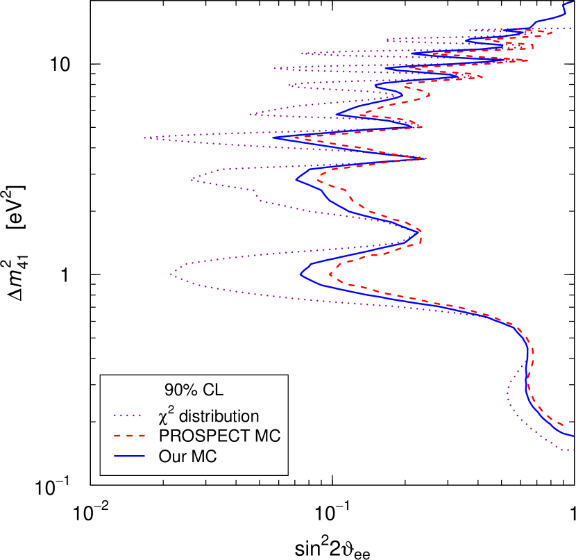
The analysis of the PROSPECT data is a useful test of our method, because the PROSPECT collaboration published the map in the ($\sin^{2}\!2\vartheta_{ee},\Delta{m}^{2}_{41}$) plane of the $\Delta\chi^{2}$ corresponding to 90% and 95% CL, that they evaluated with a Monte Carlo that takes into account all the experimental details, including the correlations of the systematic uncertainties of the binned data. Figure 1 shows the comparison of the 90% CL exclusion curves in the ($\sin^{2}\!2\vartheta_{ee},\Delta{m}^{2}_{41}$) plane obtained with the $\chi^{2}$ distribution for $\Delta\chi^{2}$ (magenta dotted), with the PROSPECT 90% CL $\Delta\chi^{2}$ map (red dashed), and with our Monte Carlo calculation (blue solid). One can see that our method yields an exclusion curve that is close to the PROSPECT one and can be considered as an acceptable approximation, especially taking into account the large improvement with respect to the exclusion curve obtained assuming the $\chi^{2}$ distribution.

Figure 2: Contours of the $1\sigma$ (blue), $2\sigma$ (red), and $3\sigma$ (green) allowed regions in the ($\sin^{2}\!2\vartheta_{ee},\Delta{m}^{2}_{41}$) plane for the four reactor spectral-ratio experiments 2 NEOS Ko et al. (2017), 2 DANSS Danilov , 2 Bugey-3 Achkar et al. (1995), and 2 PROSPECT Ashenfelter et al. (2018). The solid lines represent the contours obtained with our Monte Carlo evaluation of the distribution of $\Delta\chi^{2}$, and the dashed lines depict the contours obtained assuming the $\chi^{2}$ distribution. Also shown are the marginal $\Delta\chi^{2}$’s (black) for $\sin^{2}\!2\vartheta_{ee}$ and $\Delta{m}^{2}_{41}$, together with the $\Delta\chi^{2}$ values corresponding to $1\sigma$ (blue), $2\sigma$ (red), and $3\sigma$ (green) obtained with the $\chi^{2}$ distribution (dashed) and our Monte Carlo (solid). The best-fit points are indicated by blue crosses.

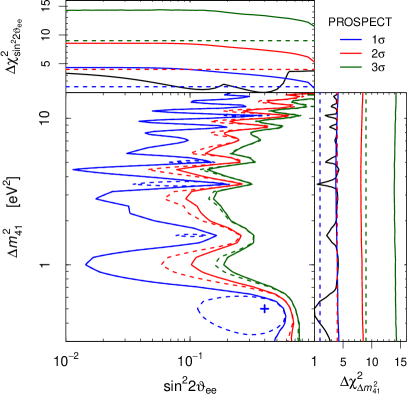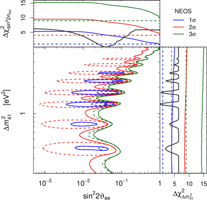
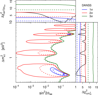
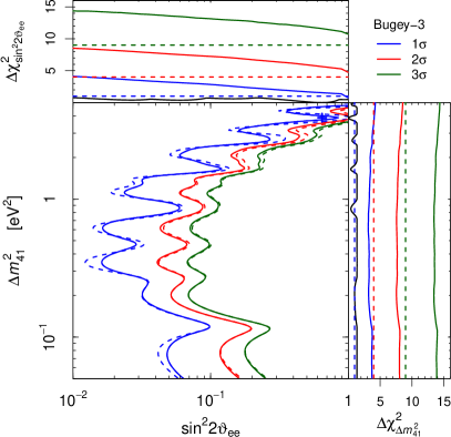
Having established the approximate reliability of our method, we present in Figure 2 the contours of the $1\sigma$, $2\sigma$, and $3\sigma$ allowed regions in the ($\sin^{2}\!2\vartheta_{ee},\Delta{m}^{2}_{41}$) plane for the four reactor spectral-ratio experiments that we take into account: NEOS Ko et al. (2017), DANSS Danilov , Bugey-3 Achkar et al. (1995), and PROSPECT Ashenfelter et al. (2018). The figures show also the marginal $\Delta\chi^{2}$’s for $\sin^{2}\!2\vartheta_{ee}$ and $\Delta{m}^{2}_{41}$ and the values of the marginal $\Delta\chi^{2}$’s corresponding to $1\sigma$, $2\sigma$, and $3\sigma$ obtained with the $\chi^{2}$ distribution (dashed) and our Monte Carlo (solid). Note that the marginal $\Delta\chi^{2}$’s corresponding to different confidence levels obtained with the $\chi^{2}$ distribution have fixed values given by Table 39.2 of Ref. Tanabashi et al. (2018) for one degree of freedom, whereas the Monte Carlo ones depend on the value of the unmarginalized parameter.

From Figure 2 one can see that in general the difference between the Monte Carlo contours and those obtained with the $\chi^{2}$ distribution is larger for small values of $\sin^{2}\!2\vartheta_{ee}$, where the $\chi^{2}$ distribution leads to undercoverage, as discussed in Ref. Agostini and Neumair . This is due to the larger probability of fitting the statistical fluctuations of the data with fake oscillations when the signal is small or absent. Correspondingly, the Monte Carlo values of the marginal $\Delta\chi^{2}_{\sin^{2}\!2\vartheta_{ee}}$’s associated with different confidence levels increase in a significant way for decreasing $\sin^{2}\!2\vartheta_{ee}$. On the other hand, the Monte Carlo values of the marginal $\Delta\chi^{2}_{\Delta{m}^{2}_{41}}$’s corresponding to different confidence levels are approximately flat, with slightly smaller values in the range of $\Delta{m}^{2}_{41}$ where the experiment is mostly sensitive. However, they are significantly larger than those obtained with the $\chi^{2}$ distribution, because for each value of $\Delta{m}^{2}_{41}$ the contribution to the marginalization of small values of $\sin^{2}\!2\vartheta_{ee}$ lead to undercoverage in the case of the $\chi^{2}$ distribution. In the range of $\Delta{m}^{2}_{41}$ where the experiment is mostly sensitive, the undercoverage is slightly smaller, because it occurs only for very small values of $\sin^{2}\!2\vartheta_{ee}$.

		$\chi^{2}$ distrib.		MC distrib.
	$\Delta\chi^{2}_{\text{NO}}$	$p$-value	$n\sigma$	$p$-value	$n\sigma$
NEOS	$6.4$	$0.041$	$2.0$	$0.2$	$1.3$
DANSS	$7.2$	$0.027$	$2.2$	$0.044$	$2.0$
Bugey-3	$1.4$	$0.5$	$0.7$	$0.9$	$0.1$
PROSPECT	$4.0$	$0.14$	$1.5$	$0.37$	$0.9$
Combined	$8.5$	$0.015$	$2.4$	$0.079$	$1.8$

Table 1: Value of $\Delta\chi^{2}_{\text{NO}}$ and the associated $p$-value and number of $\sigma$’s obtained with the $\chi^{2}$ distribution and with the Monte Carlo distribution. The lines correspond to the four reactor spectral-ratio experiments NEOS Ko et al. (2017), DANSS Danilov , Bugey-3 Achkar et al. (1995), PROSPECT Ashenfelter et al. (2018), and to the combined fit.

Figure 3: Contours of the $1\sigma$ (blue), $2\sigma$ (red), and $3\sigma$ (green) allowed regions in the ($\sin^{2}\!2\vartheta_{ee},\Delta{m}^{2}_{41}$) plane obtained with the combined analysis of the data of the four reactor spectral-ratio experiments NEOS Ko et al. (2017), DANSS Danilov , Bugey-3 Achkar et al. (1995), and PROSPECT Ashenfelter et al. (2018). The solid lines represent the contours obtained with our Monte Carlo evaluation of the distribution of $\Delta\chi^{2}$, and the dashed lines depict the contours obtained assuming the $\chi^{2}$ distribution. Also shown are the marginal $\Delta\chi^{2}$’s (black) for $\sin^{2}\!2\vartheta_{ee}$ and $\Delta{m}^{2}_{41}$, together with the $\Delta\chi^{2}$ values corresponding to $1\sigma$ (blue), $2\sigma$ (red), and $3\sigma$ (green) obtained with the $\chi^{2}$ distribution (dashed) and our Monte Carlo (solid). The blue cross indicates the best-fit point.

The Monte Carlo evaluation of the distribution of the $\Delta\chi^{2}$ allows us also to estimate reliably the statistical significance of the indication in favor of active-sterile neutrino oscillations in each experiment. This is done by considering the difference $\Delta\chi^{2}_{\text{NO}}=\chi^{2}_{\text{NO}}-\chi^{2}_{\text{min}}$, where $\chi^{2}_{\text{NO}}$ is the value of the $\chi^{2}$ obtained without neutrino oscillations. If the conditions for Wilks’ theorem Wilks (1938) hold, $\Delta\chi^{2}_{\text{NO}}$ has a $\chi^{2}$ distribution with two degrees of freedom corresponding to the two fitted parameters $\sin^{2}\!2\vartheta_{ee}$ and $\Delta{m}^{2}_{41}$. Table 1 shows the values of $\Delta\chi^{2}_{\text{NO}}$ that we obtained in the analyses of the data of the four reactor spectral-ratio experiments NEOS Ko et al. (2017), DANSS Danilov , Bugey-3 Achkar et al. (1995), and PROSPECT Ashenfelter et al. (2018). Also shown are the $p$-value of the no-oscillation hypothesis and the corresponding number of $\sigma$’s for a two-sided Gaussian deviation obtained with the $\chi^{2}$ distribution and the Monte Carlo distribution. The statistical significance of the indication in favor of active-sterile neutrino oscillations can be quantified by the smallness of the $p$-value or by the number of $\sigma$’s. One can see that for all the considered experiments this statistical significance is reduced considering the Monte Carlo distribution of $\Delta\chi^{2}_{\text{NO}}$ with respect to the $\chi^{2}$ distribution.

The NEOS indication of neutrino oscillations is strongly reduced from $2.0\sigma$ to $1.3\sigma$ using the Monte Carlo distribution instead of the $\chi^{2}$ distribution. Note that our Monte Carlo $20\%$ $p$-value is in very good approximate agreement with the 22% $p$-value estimated by the NEOS collaboration Ko et al. (2017). This is another confirmation of the validity of our method.

Using the Monte Carlo distribution instead of the $\chi^{2}$ distribution, the significance of the DANSS indication of neutrino oscillations is only slightly reduced from $2.2\sigma$ to $2.0\sigma$.

From Table 1 one can also see that the Bugey-3 experiment has clearly no indication of neutrino oscillations, independently of the assumed distribution of $\Delta\chi^{2}_{\text{NO}}$. Indeed, although the best-fit point in Figure 2 corresponds to large oscillations, all the confidence level contours are exclusion curves and the values of the marginal $\Delta\chi^{2}$’s are very small.

The PROSPECT $\chi^{2}$ has a minimum for large oscillations, as shown by Figure 2, but the value of the $\Delta\chi^{2}$ is small and in agreement with the absence of oscillations. The Monte Carlo calculation of the distribution of the $\Delta\chi^{2}$ gives a statistical significance for oscillations that is only $0.9\sigma$, and significantly smaller than the $1.5\sigma$ obtained with the $\chi^{2}$ distribution. Our Monte Carlo $p$-value of $37\%$ is not as large as the 58% obtained by the PROSPECT collaboration Ashenfelter et al. (2018), but it is much closer to it than the $14\%$ obtained with the $\chi^{2}$ distribution.

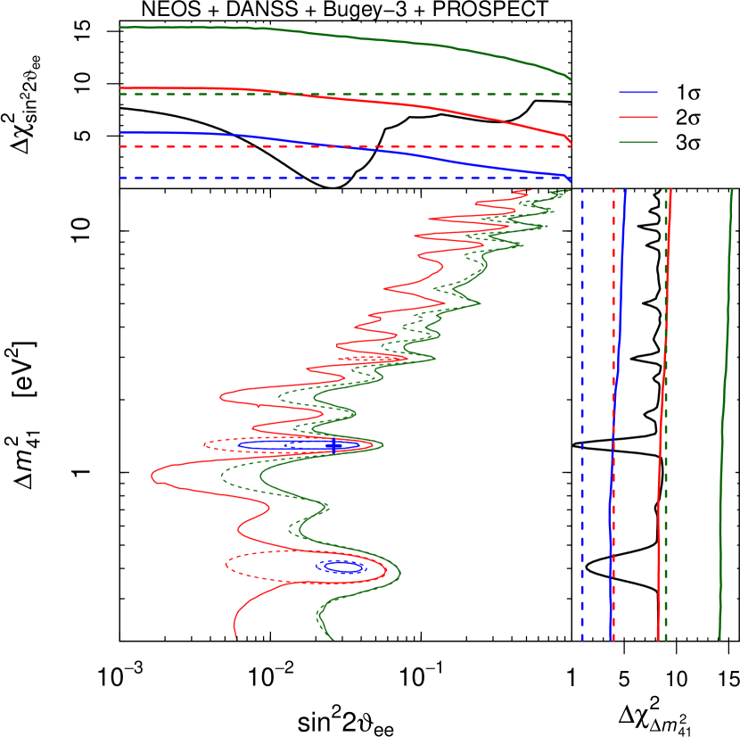
We finally performed the combined fit of the data of all the four reactor spectral-ratio experiments NEOS Ko et al. (2017), DANSS Danilov , Bugey-3 Achkar et al. (1995), and PROSPECT Ashenfelter et al. (2018). Figure 3 shows the contours of the $1\sigma$, $2\sigma$, and $3\sigma$ allowed regions in the ($\sin^{2}\!2\vartheta_{ee},\Delta{m}^{2}_{41}$) plane and the marginal $\Delta\chi^{2}$’s for $\sin^{2}\!2\vartheta_{ee}$ and $\Delta{m}^{2}_{41}$. As in Figure 2, the dashed lines correspond to the $\chi^{2}$ distribution, whereas the solid lines have been obtained with our Monte Carlo. The combined fit yields the best-fit point at $\sin^{2}\!2\vartheta_{ee}=0.026$ and $\Delta{m}^{2}_{41}=1.3\,\text{eV}^{2}$ with $\chi^{2}_{\text{min}}=183.6$ and $197$ degrees of freedom. Therefore, the fit is very good, either considering a $\chi^{2}$ distribution for $\chi^{2}_{\text{min}}$ ($75\%$ goodness of fit) or with a Monte Carlo estimation ($89\%$ goodness of fit). The best fit corresponds to the allowed regions of NEOS and DANSS at $\Delta{m}^{2}_{41}\approx 1.3\,\text{eV}^{2}$, that can be seen in Figures 2 and 2.

Figure 3 shows that the Monte Carlo allowed regions are much larger than those obtained with the $\chi^{2}$ distribution and extend to smaller values of the mixing. This means that the preference for neutrino oscillations is smaller. Indeed, from Table 1 one can see that the significance of the indication of neutrino oscillations is reduced from $2.4\sigma$ to $1.8\sigma$. Correspondingly, in Figure 3 there are several closed contours that delimit regions allowed at 90% CL, that corresponds to about $1.64\sigma$.

In conclusion, our Monte Carlo calculations show that the significance of the indication of neutrino oscillations given by the combined analysis of the reactor spectral-ratio measurements is not as large as thought before Gariazzo et al. (2018); Dentler et al. (2018); Berryman and Huber (2020); Giunti et al. using a $\chi^{2}$ distribution for $\Delta\chi^{2}$. Nevertheless, there is still an marginal $1.8\sigma$ indication in favor of active-sterile neutrino oscillations that will hopefully be resolved by new data of the ongoing DANSS Alekseev et al. (2018); Danilov , PROSPECT Ashenfelter et al. (2018), STEREO Almazan et al. (2018); Almazan Molina et al. , Neutrino-4 Serebrov et al. (2019); Serebrov and Samoilov , and SoLid Abreu et al. reactor spectral-ratio experiments.

The interpretation of the results of the experiments searching for active-sterile neutrino oscillations is currently controversial. In this situation it is important that the combined analyses of the data of different experiments are performed by calculating the appropriate distribution of the test statistic, as we have done here, in order to reach reliable information on the statistical significance of active-sterile neutrino oscillations. The quality of such analysis depends on how well the test statistic takes into account the experimental setup and the systematic uncertainties, including their correlation. To this aim it is necessary that each experimental collaboration make available all the necessary information.