Vacuum expectation values in non-trivial background space from three types of UV improved Green’s functions

Abstract

We evaluate the quantum expectation values in non-simply connected spaces by using UV improved Green’s functions proposed by Padmanabhan, Abel, and Siegel. It is found that the results from these three types of Green’s functions behave similarly under changes of scales, but have minute differences. Prospects in further applications are briefly discussed.

I Introduction

The appearance of divergences in the ultra-violet (UV) region is one of the fundamental problems in quantum field theory. The problem of UV completion is expected to be connected to quantum gravity, because the UV divergence is naively considered to be related to fine structures of spacetime.

Almost two decades ago, Padmanabhan Pad1 ; Pad2 ; Pad3 ; Pad4 ; Pad5 ; Pad6 and his collaborators SSP ; KSSP considered a UV completed propagator involving the “Planck length” as a cutoff small-length scale. Padmanabhan’s propagator was induced by the duality in the integrand kernel with a proper-time parameter. More recently, Abel and his collaborators AD ; ABM proposed their UV improved propagator, which is also inspired by the integral over modular parameter in string theory. Modification of integration measure or range was also offered by Siegel Siegel at the beginning of this century, motivated by an infinite derivative theory.

The authors who mentioned UV improved propagators studied and calculated various physical quantities mainly in homogeneous Minkowski spacetime. Because the UV behavior is believed to be concerned with quantum gravity, it will be important to study further on physical results of the UV completion in non-trivial spacetimes.

The non-trivial space that can be handled most easily is a non-simply connected space. In the present paper, Euclidean Kaluza–Klein space and space with a conical singularity are adopted as background spaces. It is already known that the vacuum energy density and the stress tensor of a scalar field can be obtained from the congruent limit of the propagator. We will examine how the “Planck length”, which is used as a common synonym for the fundamental cutoff length, works for the quantum quantities and compare the consequences arising from the three modified Green’s functions (we use this term because we use the Euclidean metric in this paper).

This paper is organized as follows. The next section contains a review of the Green’s function for a massless scalar field and an introduction of three UV improved Green’s functions, say, Padmanabhan’s type, Abel’s type, and Siegel’s type. They can be expressed by the integral form of the heat kernel of the Laplacian. In Sec. III, we consider a partially compactified space à la Kaluza-Klein. We calculate the vacuum energy density using three UV improved Green’s functions in the non-simply connected space $\mathbf{R}^{D-1}\otimes S^{1}$. The dependence of the energy densities on the ratio of the circumference of $S^{1}$ and the Planck length is shown. In Sec. IV the expectation values for the stress tensor are computed for the three types of Green’s functions in a conical space. Finally, in Sec. V we conclude with a discussion of future directions. At the end of this paper, we attach Appendices A and B, where mathematical definitions and formulas are gathered, for convenience.

II Three UV improved Green’s functions and the heat kernels in homogeneous and isotropic Euclidean space $\mathbf{R}^{D}$

Let us first recall some basic facts with standard Green’s functions and heat kernels of a flat metric Vassilevich ; Camporesi . Suppose that the standard Green’s function $G_{D}(x,x^{\prime})$ of a massless scalar field in a $D$-dimensional Euclidean space $\mathbf{R}^{D}$ satisfies

$$-\Delta_{x}{G}_{D}(x,x^{\prime})=\frac{1}{\sqrt{g}}\delta^{D}(x,x^{\prime})\,,$$ (1)

where $\Delta=\frac{1}{\sqrt{g}}\partial_{\mu}\sqrt{g}g^{\mu\nu}\partial_{\nu}$ is the Laplacian operator acting on scalar fields and $\frac{1}{\sqrt{g}}\delta^{D}(x,x^{\prime})$ is the $D$-dimensional covariant delta function.

The main tool that we use here is the heat kernel of the Laplacian. The heat kernel $K_{D}(x,x^{\prime};s)$ is introduced as a representation of the Green’s function written by using it:

$${G}_{D}(x,x^{\prime})=\int_{0}^{\infty}ds\,K_{D}(x,x^{\prime};s)\,.$$ (2)

Here, the heat kernel obeys the equation

$$\left[\frac{\partial}{\partial s}-\Delta_{x}\right]K_{D}(x,x^{\prime};s)=0\,,$$ (3)

with the boundary condition $\lim_{s\rightarrow 0}K_{D}(x,x^{\prime};0)=\frac{1}{\sqrt{g}}\delta^{D}(x,x^{\prime})$. Subsequently, the heat kernel in $\mathbf{R}^{D}$ is found to be

$$K_{D}(x,x^{\prime};s)=\int\frac{d^{D}p}{(2\pi)^{D}}\exp\left[-sp^{2}\right]e^{ip\cdot(x-x^{\prime})}=\frac{1}{(4\pi s)^{D/2}}\exp\left({-\frac{w^{2}}{4s}}\right)\,,$$ (4)

and the massless Green’s function reads

$$G_{D}(x,x^{\prime})=\frac{\Gamma\left({\textstyle\frac{D-2}{2}}\right)}{4\pi^{D/2}w^{D-2}}\equiv G_{D}(w)\,,$$ (5)

where $w\equiv\sqrt{\scriptstyle(x-x^{\prime})\cdot(x-x^{\prime})}$ and $\Gamma(z)$ is the gamma function.

Next, we consider UV improved heat kernels and Green’s functions. Padmanabhan advocated a UV modified heat kernel Pad1 ; Pad2 ; Pad3 ; Pad4 ; Pad5 ; Pad6

$$K^{(P)}_{D}(x,x^{\prime};s)=K_{D}(x,x^{\prime};s)\exp\left(-\frac{l_{p}^{2}}{4s}\right)\,,$$ (6)

where $l_{p}$ is interpreted as the Planck length. Obviously, Padmanabhan’s heat kernel leads to the Green’s function $G_{D}^{(P)}(w)$ in $\mathbf{R}^{D}$, which can be written as

$$G_{D}^{(P)}(w)=G_{D}\left({\textstyle\sqrt{w^{2}+l_{p}^{2}}}\right)\,.$$ (7)

This shows the simplest introduction of the fundamental length $l_{p}$ in the Green’s function of Padmanabhan’s type and it give rise to the UV completion.

Recently, Abel et al. considered another UV modified heat kernel AD ; ABM , which can be regarded as

$$K^{(A)}_{D}(x,x^{\prime};s)=K_{D}(x,x^{\prime};{\textstyle s+\frac{l_{p}^{4}}{4s}})\,.$$ (8)

In this case, the Green’s function can be expressed as

$$G^{(A)}_{D}(x,x^{\prime})=\int_{l_{p}^{2}}^{\infty}dT\frac{T}{\sqrt{T^{2}-l_{p}^{4}}}K_{D}(x,x^{\prime};T)\,,$$ (9)

after the change of integration variable. Performing the integral yields a complicate form for the massless Green’s function of Abel’s type in $\mathbf{R}^{D}$:

$$G^{(A)}_{D}(x,x^{\prime}) = \frac{1}{2^{D}\pi^{(D-1)/2}l_{p}^{D-2}}\left[\frac{\Gamma({\textstyle\frac{D-2}{4})}}{2\Gamma({\textstyle\frac{D}{4}})}\,{}_{1}F_{2}({\textstyle\frac{D-2}{4};\frac{1}{2},\frac{D}{4};\frac{w^{4}}{64l_{p}^{4}}})-\right.$$ (10)

$$\qquad\qquad\qquad\qquad\left.\frac{w^{2}}{8l_{p}^{2}}\frac{\Gamma({\textstyle\frac{D}{4}})}{\Gamma({\textstyle\frac{D+2}{4}})}\,{}_{1}F_{2}({\textstyle\frac{D}{4};\frac{3}{2},\frac{D+2}{4};\frac{w^{4}}{64l_{p}^{4}}})\right]\,,$$

where ${}_{p}F_{q}$ is the hypergeometric function. For $D=4$, the expression (10) reads

$$G^{(A)}_{4}(x,x^{\prime})=\frac{1}{32\pi l_{p}^{2}}\left[I_{0}({\textstyle\frac{w^{2}}{4l_{p}^{2}}})-\mathbf{L}_{0}({\textstyle\frac{w^{2}}{4l_{p}^{2}}})\right]\,,$$ (11)

where $I_{\nu}(z)$ is the modified Bessel function of the first kind and $\mathbf{L}_{\nu}(z)$ is the modified Struve function (see Appendix A).

Siegel suggested a simple UV completion Siegel , which is achieved by

$$K^{(S)}_{D}(x,x^{\prime};s)=K_{D}(x,x^{\prime};s+l_{p}^{2})\,.$$ (12)

Then, the Siegel-type Green’s function for a massless scalar field in $\mathbf{R}^{D}$ reads

$$G^{(S)}_{D}(x,x^{\prime})=\frac{1}{4\pi^{D/2}w^{D-2}}\gamma({\textstyle\frac{D-2}{2},\frac{w^{2}}{4l_{p}^{2}}})=\frac{1}{4\pi^{D/2}w^{D-2}}\left[\Gamma({\textstyle\frac{D-2}{2}})-\Gamma({\textstyle\frac{D-2}{2},\frac{w^{2}}{4l_{p}^{2}}})\right]\,,$$ (13)

where $\gamma(z,\alpha)$ and $\Gamma(z,\alpha)$ are the incomplete gamma functions which are defined by $\gamma(z,\alpha)\equiv\int_{0}^{\alpha}t^{z-1}e^{-t}dt$ and $\Gamma(z,\alpha)\equiv\int_{\alpha}^{\infty}t^{z-1}e^{-t}dt$, respectively.

Obviously, taking the limit of $l_{p}\rightarrow 0$, we find

$$\lim_{l_{p}\rightarrow 0}G^{(P)}_{D}(x,x^{\prime})=\lim_{l_{p}\rightarrow 0}G^{(A)}_{D}(x,x^{\prime})=\lim_{l_{p}\rightarrow 0}G^{(S)}_{D}(x,x^{\prime})=G_{D}(x,x^{\prime})\,.$$ (14)

In the opposite limit, $x^{\prime}\rightarrow x$, we get finite results immediately as

$$\lim_{x^{\prime}\rightarrow x}G^{(P)}_{D}(x,x^{\prime}) = \frac{\Gamma\left({\textstyle\frac{D-2}{2}}\right)}{4\pi^{D/2}l_{p}^{D-2}}\,,$$

$$\lim_{x^{\prime}\rightarrow x}G^{(A)}_{D}(x,x^{\prime}) = \frac{\Gamma({\textstyle\frac{D-2}{4}})}{2^{D+1}\pi^{(D-1)/2}\Gamma({\textstyle\frac{D}{4}})l_{p}^{D-2}}\,,$$

$$\lim_{x^{\prime}\rightarrow x}G^{(S)}_{D}(x,x^{\prime}) = \frac{1}{2^{D-1}(D-2)\pi^{D/2}l_{p}^{D-2}}\,,$$ (15)

and find that they are $O(l_{p}^{2-D})$ as expected.

In the following sections, we generalize three UV improved Green’s functions to treat quantum quantities in non-simply connected space.

III UV improved Green’s functions and vacuum energy density in a partially compactified space $\mathbf{R}^{D-1}\otimes S^{1}$

We consider a $D$-dimensional space whose metric is given by

$$ds^{2}=\sum_{i=1}^{D-1}dz_{i}^{2}+dy^{2}\,,$$ (16)

where the coordinate $y$ is the coordinate on a circle ($S^{1}$) and we assume that $0\leq y<L$, where $L$ is the circumference of the circle. The periodic boundary condition in the direction of $y$ is supposed to be applied on the massless scalar, i.e., $\phi(y+L)=\phi(y)$. In this space, $\mathbf{R}^{D-1}\otimes S^{1}$, the heat kernel for the standard massless scalar field takes the form

$$K_{D}(z,z^{\prime},y,y^{\prime};s) = \sum_{n=-\infty}^{\infty}\frac{1}{L}\int\frac{d^{D-1}p}{(2\pi)^{D-1}}\exp\left[-s\left({\textstyle p^{2}+\frac{4\pi^{2}n^{2}}{L^{2}}}\right)\right]e^{ip\cdot(z-z^{\prime})+i2\pi n(y-y^{\prime})/L}$$ (17)

$$= \frac{1}{(4\pi s)^{D/2}}\sum_{n=-\infty}^{\infty}\exp\left[-\frac{\zeta^{2}+(\eta-nL)^{2}}{4s}\right]\equiv K_{D}(\zeta,\eta;s)\,,$$

where $\zeta=\sqrt{\scriptstyle(z-z^{\prime})\cdot(z-z^{\prime})}$ and $\eta=y-y^{\prime}$. The second expression with the periodic summation can be derived with the aid of the formula of the theta function (see Appendix A) as well as from the method of images. We should also notice that the limit $L\rightarrow\infty$ yields the heat kernel in $\mathbf{R}^{D}$.

In the subsections below, we study the Green’s functions of Padmanabhan-type, Abel-type, and Siegel-type in $\mathbf{R}^{D-1}\otimes S^{1}$, and the vacuum energies extracted from them.

III.1 Vacuum energy from Padmanabhan-type Green’s function

Padmanabhan-type Green’s function in $\mathbf{R}^{D-1}\otimes S^{1}$ is found to be

$$K_{D}^{(P)}(\zeta,\eta;s)=K_{D}({\textstyle\sqrt{\zeta^{2}+l_{p}^{2}}},\eta;s)\,.$$ (18)

We can calculate the effective action $W$ from the trace of heat kernel. In the present case, the effective action in terms of Padmanabhan’s heat kernel becomes

$$W_{D}^{(P)}=\frac{1}{2}L\int d^{D-1}z\int_{0}^{\infty}\frac{ds}{s}K_{D}^{(P)}(0,0;s)=\frac{1}{2}L\int d^{D-1}z\int_{0}^{\infty}\frac{ds}{s}K_{D}(l_{p},0;s)\,.$$ (19)

It is noteworthy that, because of the UV modification, a cutoff in $s$-integration or an additional power of $s$ in the integrand is unnecessary.

Consequently, the one-loop vacuum energy density $U_{D}^{(P)}=-W_{D}^{(P)}/V_{D-1}$, where $V_{D-1}$ is the $(D-1)$-dimensional volume, reads

$$U_{D}^{(P)}(L) = -\frac{1}{2\pi^{D/2}L^{D-1}}\int_{0}^{\infty}dt\,t^{D/2-1}\sum_{n=-\infty}^{\infty}\exp\left[-\left({\textstyle n^{2}+\frac{l_{p}^{2}}{L^{2}}}\right)t\right]$$ (20)

$$= -\frac{1}{2\pi^{D/2}L^{D-1}}\int_{0}^{\infty}dt\,t^{D/2-1}\vartheta_{3}({0,it/\pi})\exp\left[-\frac{l_{p}^{2}}{L^{2}}t\right]\,,$$

where $\vartheta_{3}$ denotes the Jacobi theta function (see Appendix A). Integrating the series by term, we find

$$U_{D}^{(P)}(L) = -\frac{\Gamma(D/2)}{2\pi^{D/2}}\sum_{n=-\infty}^{\infty}\frac{L}{\left(l_{p}^{2}+n^{2}L^{2}\right)^{D/2}}$$ (21)

$$= -\frac{\Gamma(D/2)L}{2\pi^{D/2}l_{p}^{D}}-\frac{\Gamma(D/2)}{\pi^{D/2}}\sum_{n=1}^{\infty}\frac{L}{\left(l_{p}^{2}+n^{2}L^{2}\right)^{D/2}}\,.$$

Since the first term in the last expression is the large $L$ limit of $U_{D}^{(P)}$, we subtract it and define the refined (or “renormalized”) effective potential

$$\bar{U}_{D}^{(P)}(L)=U_{D}^{(P)}(L)-U_{D}^{(P)}(\infty)=-\frac{\Gamma(D/2)}{\pi^{D/2}}\sum_{n=1}^{\infty}\frac{L}{\left(l_{p}^{2}+n^{2}L^{2}\right)^{D/2}}\,.$$ (22)

It should be noticed that, even if the one-loop vacuum energy density $U_{D}^{(P)}$ is finite due to UV completion, the huge contribution of the order of $l_{p}^{-D}$ should be renormalized or compensated by some method. This attitude is taken in the subsequent sections. We will come back to the discussion in Sec. V.

Now, the known result on standard one-loop scalar energy density for the Kaluza-Klein theory, $-\frac{\Gamma(D/2)\zeta_{R}(D)}{\pi^{D/2}L^{D-1}}$ (where $\zeta_{R}(z)$ is the Riemann’s zeta function) CW , can be obtained by taking the limit $l_{p}\rightarrow 0$. Expanding $\bar{U}_{D}^{(P)}$ in terms of a small $l_{p}/L$, we obtain

$$\bar{U}_{D}^{(P)}(L) = -\frac{\Gamma(D/2)}{\pi^{D/2}L^{D-1}}\sum_{n=1}^{\infty}\frac{1}{n^{D}}\sum_{k=0}^{\infty}\frac{(-1)^{k}\Gamma(k+D/2)}{\Gamma(D/2)k!}\left(\frac{l_{p}^{2}}{n^{2}L^{2}}\right)^{k}$$ (23)

$$= -\frac{1}{\pi^{D/2}L^{D-1}}\sum_{k=0}^{\infty}\frac{(-1)^{k}\Gamma(k+D/2)\zeta(D-2k)}{k!}\left(\frac{l_{p}^{2}}{L^{2}}\right)^{k}\,.$$

On the other hand, we can obtain another expression by series

$$\bar{U}_{D}^{(P)}(L)=-\frac{\Gamma((D-1)/2)}{2\pi^{(D-1)/2}l_{p}^{D-1}}-2\sum_{n=1}^{\infty}\left(\frac{n}{l_{p}L}\right)^{(D-1)/2}K_{(D-1)/2}(2\pi l_{p}n/L)\,,$$ (24)

where, $K_{\nu}(z)$ is the modified Bessel function of the second kind (see Appendix A), which shows that $\bar{U}_{D}^{(P)}(0)=-\frac{\Gamma((D-1)/2)}{2\pi^{(D-1)/2}l_{p}^{D-1}}$ is finite.

Further, we consider a complex massless scalar field $\Phi$ and assume a general boundary condition

$$\Phi(y+L)=e^{i\delta}\Phi(y)\,.$$ (25)

Then, the vacuum energy density can be obtained as

$$\bar{U}_{D}^{(P)}(L,\delta)=-\frac{2\Gamma(D/2)}{\pi^{D/2}}\sum_{n=1}^{\infty}\frac{L\cos(n\delta)}{\left(l_{p}^{2}+n^{2}L^{2}\right)^{D/2}}\,.$$ (26)

Of course, $\bar{U}_{D}^{(P)}(L,0)$ coincides with $\bar{U}_{D}^{(P)}(L)$. Additionally, $\bar{U}_{D}^{(P)}(L,\delta)$ has a closed form without integrals and summations provided that $D$ is an even integer. For instance, for $D=4$, one can find

$${\textstyle\bar{U}_{4}^{(P)}(L,\delta)=\frac{L}{2\pi^{2}l_{p}^{4}}-\frac{1}{4\pi l_{p}^{3}}\frac{\cosh[l_{p}(\pi-\delta)/L]+(l_{p}/L)\delta\sinh[l_{p}(\pi-\delta)/L]}{\sinh(l_{p}\pi/L)}-\frac{1}{4l_{p}^{2}L}\frac{\cosh(l_{p}\delta/L)}{\sinh^{2}(l_{p}\pi/L)}}\,.$$ (27)

Numeric analyses will be given in a later subsection, after derivation of vacuum energy in terms of all the three types of Green’s functions, where we compare the result from each scheme of UV completion.

III.2 Vacuum energy from Abel-type Green’s function

We define the effective action in $\mathbf{R}^{D-1}\otimes S^{1}$ from Abel’s heat kernel, that is.

$$W_{D}^{(A)} = \frac{1}{2}L\int d^{D-1}z\,\,\frac{1}{2}\int_{0}^{\infty}\frac{ds}{s}K_{D}^{(A)}(0,0;s)=\frac{1}{2}L\int d^{D-1}z\int_{l_{p}^{2}/2}^{\infty}\frac{ds}{s}K_{D}^{(A)}(0,0;s)$$ (28)

$$= \frac{1}{2}L\int d^{D-1}z\int_{l_{p}^{2}}^{\infty}\frac{dT}{\sqrt{T^{2}-l_{p}^{4}}}K_{D}(0,0;T)\,.$$

It is notable that the factor $1/2$ in front of the integration over $s$ after the first equal sign comes from the exact duality $s\leftrightarrow l_{p}^{4}/(4s)$ in this one-loop integration. In a similar way to Padmanabhan’s case, we define the refined vacuum energy density and the expression for this vacuum energy is

$$\bar{U}_{D}^{(A)}(L) = -\frac{1}{2\pi^{D/2}L^{D-1}}\int_{0}^{\frac{L^{2}}{4l_{p}^{2}}}dt\frac{t^{D/2-1}}{\sqrt{1-\frac{16l_{p}^{4}}{L^{4}}t^{2}}}\left(\sum_{n=-\infty}^{\infty}e^{-n^{2}t}-1\right)$$ (29)

$$= -\frac{1}{2\pi^{D/2}L^{D-1}}\int_{0}^{\frac{L^{2}}{4l_{p}^{2}}}dt\frac{t^{D/2-1}}{\sqrt{1-\frac{16l_{p}^{4}}{L^{4}}t^{2}}}\left[\vartheta_{3}(0,it/\pi)-1\right]\,.$$

For a complex scalar field with twisted boundary condition (25), the vacuum energy density becomes

$$\bar{U}_{D}^{(A)}(L,\delta) = -\frac{1}{\pi^{D/2}L^{D-1}}\int_{0}^{\frac{L^{2}}{4l_{p}^{2}}}dt\frac{t^{D/2-1}}{\sqrt{1-\frac{16l_{p}^{4}}{L^{4}}t^{2}}}\left(\sum_{n=-\infty}^{\infty}e^{-n^{2}t+in\delta}-1\right)$$ (30)

$$= -\frac{1}{\pi^{D/2}L^{D-1}}\int_{0}^{\frac{L^{2}}{4l_{p}^{2}}}dt\frac{t^{D/2-1}}{\sqrt{1-\frac{16l_{p}^{4}}{L^{4}}t^{2}}}\left[\vartheta_{3}(\delta/(2\pi),it/\pi)-1\right]\,.$$

III.3 Vacuum energy from Siegel-type Green’s function

The effective action in $\mathbf{R}^{D-1}\otimes S^{1}$ from Siegel’s heat kernel can be obtained by

$$W_{D}^{(S)}=\frac{1}{2}L\int d^{D-1}z\int_{0}^{\infty}\frac{ds}{s}K_{D}^{(S)}(0,0;s)=\frac{1}{2}L\int d^{D-1}z\int_{l_{p}^{2}}^{\infty}\frac{ds}{s}K_{D}(0,0;s)\,.$$ (31)

Similarly to the former cases, we define the refined vacuum energy density and the expression for is is found to be

$$\bar{U}_{D}^{(S)}(L) = -\frac{1}{2\pi^{D/2}L^{D-1}}\int_{0}^{\frac{L^{2}}{l_{p}^{2}}}dt\,t^{D/2-1}\left(\sum_{n=-\infty}^{\infty}e^{-n^{2}t}-1\right)$$ (32)

$$= -\frac{1}{2\pi^{D/2}L^{D-1}}\int_{0}^{\frac{L^{2}}{l_{p}^{2}}}dt\,t^{D/2-1}\left[\vartheta_{3}(0,it/\pi)-1\right]\,,$$

and the vacuum energy density from the twisted scalar field becomes

$$\bar{U}_{D}^{(S)}(L,\delta) = -\frac{1}{\pi^{D/2}L^{D-1}}\int_{0}^{\frac{L^{2}}{l_{p}^{2}}}dt\,t^{D/2-1}\left(\sum_{n=-\infty}^{\infty}e^{-n^{2}t+in\delta}-1\right)$$ (33)

$$= -\frac{1}{\pi^{D/2}L^{D-1}}\int_{0}^{\frac{L^{2}}{l_{p}^{2}}}dt\,t^{D/2-1}\left[\vartheta_{3}(\delta/(2\pi),it/\pi)-1\right]\,.$$

III.4 Numerical comparison of three vacuum energy densities

In this subsection, we show the numerical results for the three types of vacuum energy in the case of $D=5$.

Fig. 1 shows the dependence of the vacuum energies on the magnitude of the Planck length, $l_{p}/L$. The value of $L^{4}\bar{U}_{5}$ is $-\frac{3\zeta(5)}{4\pi^{2}}=-0.0787\cdots$ in the limit of $l_{p}\rightarrow 0$. Each dependence on $l_{p}/L$ is different. The value of $L^{4}\bar{U}_{5}$ of Abel-type takes a minimum at a finite $l_{p}$. The value of $L^{4}\bar{U}_{5}$ of Siegel-type varies moderately near $l_{p}/L\ll 1$. Note that, as we simply take a common scale $l_{p}$ for three cases, the comparison in values at the same $l_{p}/L$ in the figure has only qualitative meanings.

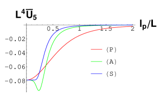
Figure 1: The vacuum energy densities regulated as $L^{4}\bar{U}_{5}$ are plotted against the Planck length $l_{p}$ divided by the circumference $L$ of $S^{1}$. The red curve indicates the Padmanabhan-type, the green curve indicates the Abel-type, and the blue curve indicates the Siegel-type.

Fig. 2 shows the vacuum energy densities $l_{p}^{4}\bar{U}_{5}$ as functions of $L/l_{p}$. All the vacuum energy densities calculated from three UV improved Green’s functions have finite values at $L=0$. All of the absolute value of vacuum energy densities are monotonically decreasing as functions of $L$. The deviation from the standard case without the fundamental scale becomes large at $L/l_{p}<1$. The comparison of absolute values has little meaning, because the Planck length for each three scheme is basically defined as an individual value. For large $L/l_{p}$, however, all the values for the energy densities are indistinguishable as expected.

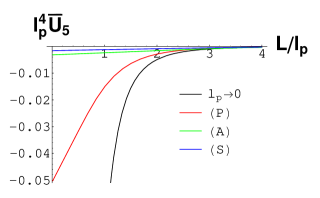
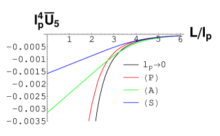
(a)                                                                       (b)

Figure 2: The vacuum energy densities $l_{p}^{4}\bar{U}_{5}$ are plotted against the circumference $L$ of $S^{1}$ divided by the Planck length $l_{p}$. The black curve indicates the usual case, i.e., the case that the Planck length is set to zero, the red curve indicates the Padmanabhan-type, the green curve indicates the Abel-type, and the blue curve indicates the Siegel-type. The left plot (a) shows the range $L/l_{p}<4$, while the right plot (b) shows the range $L/l_{p}<6$ with an enlarged vertical axis.

The vacuum energy densities of a complex scalar field with the twisted boundary condition $\bar{U}_{5}(L,\delta)$ are exhibited in Fig. 3. If we assume that $L$ is kept at a finite value, a finite value of the Planck length makes the effective potential with respect to $\delta$ flat in all the three cases. The twisted parameter can be regarded as a dynamical variable, which comes from the vacuum gauge field on $S^{1}$ Hosotani . Furthermore, the possibility of the identification of such a degree of freedom as an inflaton has been proposed by several authors ACCR ; IKLM . Because the flat potential would be suitable for such inflationary scenarios, it can be said that the effect of UV cutoff may also be relevant to the cosmological dynamics.

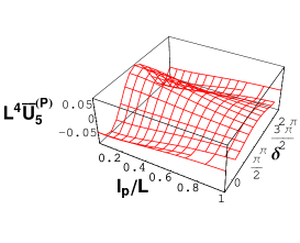
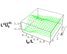
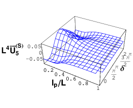
(P)                                             (A)                                             (S)

Figure 3: Plots of the vacuum energy densities of a complex scalar field with the twisted boundary condition for (P) Padmanabhan-type, (A) Abel-type, and (S) Siegel-type.

IV UV improved quantum stress tensors in a conical space

Let us turn to another non-trivial space, a conical space or space with a conical defect. We take the coordinates for a conical space as

$$ds^{2}=\sum_{i=1}^{D-2}(dz^{i})^{2}+dr^{2}+\frac{r^{2}}{\nu^{2}}d\theta^{2}\,,$$ (34)

where $\nu$ is a constant greater than unity. This metric is equivalent to

$$ds^{2}=\sum_{i=1}^{D-2}(dz^{i})^{2}+dr^{2}+r^{2}d\tilde{\theta}^{2}\,,$$ (35)

where the range of $\tilde{\theta}$ is $0<\tilde{\theta}\leq 2\pi/\nu$. This metric adequately describes a locally flat Euclidean space except for the coordinate origin if $\nu\neq 1$. A space with a deficit angle is often employed as a model space around a mathematically idealized straight cosmic string Vilenkin .

The standard heat kernel in a conical space without fundamental length is known CKV ; Moreira and presented in the form in terms of $x=(r,\theta,z^{i})$ and $x^{\prime}=(r^{\prime},\theta^{\prime},z^{\prime i})$,

$$K_{D,\nu}(x,x^{\prime};s) = \frac{\nu}{(4\pi s)^{D/2}}\sum_{m=-\infty}^{\infty}e^{im\varphi}I_{\nu|m|}\left(\frac{rr^{\prime}}{2s}\right)\exp\left[-\frac{r^{2}+{r^{\prime}}^{2}+\zeta^{2}}{4s}\right]$$ (36)

$$\equiv K_{D,\nu}(r,r^{\prime},\varphi,\zeta;s)\,,$$

where $\varphi=\theta-\theta^{\prime}$ and $\zeta=|z-z^{\prime}|$. By using the formula

$$\sum_{m=-\infty}^{\infty}e^{im\varphi}I_{\nu|m|}(z)=\frac{1}{\nu}\exp[{z\cos(\varphi/\nu)}]$$

$$\qquad+\frac{1}{2\pi}\int_{0}^{\infty}e^{-z\cosh v}\left[\frac{\sin(\varphi-\nu\pi)}{\cosh\nu v-\cos(\varphi-\nu\pi)}-\frac{\sin(\varphi+\nu\pi)}{\cosh\nu v-\cos(\varphi+\nu\pi)}\right]dv\,,$$ (37)

which can be derived from the integral form of the modified Bessel function

$$I_{\mu}(z)=\frac{1}{2\pi}\int_{-\pi}^{\pi}e^{z\cos\theta}\cos\mu\theta\,d\theta-\frac{\sin\mu\pi}{\pi}\int_{0}^{\infty}e^{-z\cosh v-\mu v}\,dv\,,$$ (38)

the heat kernel $K_{D,\nu}(r,r^{\prime},\varphi,\zeta;s)$ can be recast in the form

$$K_{D,\nu}(r,r^{\prime},\varphi,\zeta;s)={\textstyle\frac{1}{(4\pi s)^{D/2}}}\exp\left[{\textstyle-\frac{r^{2}+{r^{\prime}}^{2}-2rr^{\prime}\cos\tilde{\varphi}+\zeta^{2}}{4s}}\right]$$

$$\,+{\textstyle\frac{e^{-\frac{r^{2}+{r^{\prime}}^{2}+\zeta^{2}}{4s}}}{2\pi(4\pi s)^{D/2}}}\int_{0}^{\infty}e^{-\frac{rr^{\prime}}{2s}\cosh v}\left[{\textstyle\frac{\nu\sin\nu(\tilde{\varphi}-\pi)}{\cosh\nu v-\cos\nu(\tilde{\varphi}-\pi)}-\frac{\nu\sin\nu(\tilde{\varphi}+\pi)}{\cosh\nu v-\cos\nu(\tilde{\varphi}+\pi)}}\right]dv\,,$$ (39)

where $\tilde{\varphi}=\varphi/\nu$.

The first term in the right hand side of (39) coincides with the heat kernel $K_{D}(x,x^{\prime};s)$ in the locally flat space (35). One can also find that the expression in the brackets in the second term in the right hand side of (39) vanishes when $\nu=1$. Therefore, it is convenient to define the refined heat kernel $\bar{K}_{D,\nu}(x,x^{\prime};s)\equiv{K}_{D,\nu}(x,x^{\prime};s)-{K}_{D}(x,x^{\prime};s)$, i.e.,

$$\bar{K}_{D,\nu}(x,x^{\prime};s) = \bar{K}_{D,\nu}(r,r^{\prime},\varphi,\zeta;s)$$ (40)

$$\equiv {\textstyle\frac{e^{-\frac{r^{2}+{r^{\prime}}^{2}+\zeta^{2}}{4s}}}{2\pi(4\pi s)^{D/2}}}\int_{0}^{\infty}e^{-\frac{rr^{\prime}}{2s}\cosh v}\left[{\textstyle\frac{\nu\sin\nu(\tilde{\varphi}-\pi)}{\cosh\nu v-\cos\nu(\tilde{\varphi}-\pi)}-\frac{\nu\sin\nu(\tilde{\varphi}+\pi)}{\cosh\nu v-\cos\nu(\tilde{\varphi}+\pi)}}\right]dv\,.$$

Now, we introduce three types of refined heat kernels in the conical space, as the previously-used way. They are:

$$\bar{K}_{D,\nu}^{(P)}(r,r^{\prime},\varphi,\zeta;s) = \bar{K}_{D,\nu}(r,r^{\prime},\varphi,{\textstyle\sqrt{\zeta^{2}+l_{p}^{2}}};s)$$ (41)

$$\bar{K}_{D,\nu}^{(A)}(r,r^{\prime},\varphi,\zeta;s) = \bar{K}_{D,\nu}(r,r^{\prime},\varphi,\zeta;{\textstyle s+\frac{l_{p}^{4}}{4s}})$$ (42)

$$\bar{K}_{D,\nu}^{(S)}(r,r^{\prime},\varphi,\zeta;s) = \bar{K}_{D,\nu}(r,r^{\prime},\varphi,\zeta;s+l_{p}^{2})\,.$$ (43)

The expectation value of the quantum stress tensor operator for a massless scalar field is given by the limit, as in the case with the standard Green’s function CKV ; Moreira ; Linet ; FS ; Smith ; SH

$$\langle T^{\rho}_{\sigma}\rangle^{(*)}=\lim_{x^{\prime}\rightarrow x}D^{\rho}_{\sigma}\bar{G}_{D,\nu}^{(*)}(x,x^{\prime})\qquad({\textstyle(*)=(P),(A),\mbox{~{}and~{}}(S)})\,,$$ (44)

where $\bar{G}_{D,\nu}^{(*)}(x,x^{\prime})=\int_{0}^{\infty}\bar{K}_{D,\nu}^{(*)}(x,x^{\prime};s)ds$ and $D^{\rho}_{\sigma}$ is the second order differential operator

$$D^{\rho}_{\sigma}\equiv(1-2\xi)\nabla^{\rho}\nabla_{\sigma^{\prime}}-\left(\frac{1}{2}-2\xi\right)\delta^{\rho}_{\sigma}\nabla^{\lambda}\nabla_{\lambda^{\prime}}-2\xi(\nabla^{\rho}\nabla_{\sigma}-\delta^{\rho}_{\sigma}\nabla^{\lambda}\nabla_{\lambda})\,.$$ (45)

Here, $\nabla_{\sigma}$ stands for a covariant derivative and $\xi$ is the coupling between the scalar field and the Ricci curvature $R$, which modified the scalar Laplacian $-\Delta\rightarrow-\Delta+\xi R$. In the conical space presently considered, the curvature is zero everywhere outside the conical singularity and the heat kernels and Green’s functions are unchanged. Thus, the aforementioned relation $\bar{G}_{D,\nu}^{(*)}(x,x^{\prime})=\int_{0}^{\infty}\bar{K}_{D,\nu}^{(*)}(x,x^{\prime};s)ds$ is held even in the case of $\xi\neq 0$.

Hereafter, we concentrate ourselves on the case with $D=4$, unless especially mentioned on $D$. As in the preceding section, the numerical estimation will be exhibited all at once in the last subsection.

IV.1 The refined Green’s function and quantum stress tensor

It is known that the standard, full (not refined) Green’s function without a cutoff scale in a conical space can be written in a simple closed form for $D=4$ Smith . Thus, the Padmanabhan-type Green’s function is easily obtained by the replacement $\zeta\rightarrow{\sqrt{\zeta^{2}+l_{p}^{2}}}$ as

$$G_{4,\nu}^{(P)}(x,x^{\prime})=\frac{1}{8\pi^{2}rr^{\prime}\sinh u}\frac{\nu\sinh\nu u}{\cosh\nu u-\cos\nu\tilde{\varphi}}\,,$$ (46)

where $\cosh u=\frac{r^{2}+r^{\prime 2}+\zeta^{2}+l_{p}^{2}}{2rr^{\prime}}$ or $\sinh\frac{u}{2}=\sqrt{\frac{(r-r^{\prime})^{2}+\zeta^{2}+l_{p}^{2}}{4rr^{\prime}}}$. As for the Padmanabhan-type vacuum averages, the use of this expression is easily handled.

First of all, we consider the vacuum expectation value of $\phi^{2}$ in the conical space Smith . In the present case, this is given by

$$\langle\phi^{2}\rangle^{(P)}(x)=\bar{G}_{4,\nu~{}}^{(P)}(x,x)\,,$$ (47)

where

$$\bar{G}_{4,\nu}^{(P)}(x,x^{\prime})=G_{4,\nu}^{(P)}(x,x^{\prime})-G_{4,1}^{(P)}(x,x^{\prime})\,.$$ (48)

A straightforward calculation with the expression (46) yields

$$\langle\phi^{2}\rangle^{(P)}(r)=\frac{1}{4\pi^{2}l_{p}^{2}}\left(f_{1}-1\right)\,,$$ (49)

where

$$f_{1}\equiv\frac{\nu l_{p}\coth\left(\nu\sinh^{-1}\frac{l_{p}}{2r}\right)}{\sqrt{l_{p}^{2}+4r^{2}}}\,.$$ (50)

It is worth noting that $f_{1}\equiv 1$ for $\nu=1$, while $\lim_{l_{p}/r\rightarrow 0}f_{1}=1$ and $\lim_{l_{p}/r\rightarrow\infty}f_{1}=\nu$ for $\nu>1$.

For small $l_{p}^{2}/r^{2}$, we find

$$\langle\phi^{2}\rangle^{(P)}(r)=\frac{\nu^{2}-1}{48\pi^{2}r^{2}}\left(1-\frac{(\nu^{2}+11)l_{p}^{2}}{60r^{2}}+O(l_{p}^{4}/r^{4})\right)\,.$$ (51)

Therefore, the effect of the Planck length vanishes far from the conical singularity sitting on the origin. Of course, the limit of $l_{p}=0$ gives the standard result in a conical space Smith .

Now, we consider the quantum stress tensor of Padmanabhan-type in the conical space. Using the formula (44), we obtain

$$\langle T^{r}_{r}\rangle^{(P)} = \frac{1}{\pi^{2}l_{p}^{4}}\left[-\frac{r^{2}}{l_{p}^{2}+4r^{2}}f_{3}+\frac{l_{p}^{4}-8l_{p}^{2}r^{2}-12r^{4}}{6(l_{p}^{2}+4r^{2})^{2}}f_{2}-\frac{2l_{p}^{4}+5l_{p}^{2}r^{2}+6r^{4}}{3(l_{p}^{2}+4r^{2})^{2}}f_{1}+\frac{1}{2}\right]$$ (52)

$$+\frac{1}{\pi^{2}l_{p}^{2}}\left(\xi-\frac{1}{6}\right)\frac{f_{2}-f_{1}}{l_{p}^{2}+4r^{2}}\,,$$

$$\langle T^{\tilde{\theta}}_{\tilde{\theta}}\rangle^{(P)} = \frac{1}{\pi^{2}l_{p}^{4}}\left[\frac{l_{p}^{2}+3r^{2}}{3(l_{p}^{2}+4r^{2})}f_{3}-\frac{l_{p}^{4}+16l_{p}^{2}r^{2}+36r^{4}}{6(l_{p}^{2}+4r^{2})^{2}}f_{2}-\frac{2l_{p}^{4}+11l_{p}^{2}r^{2}+18r^{4}}{3(l_{p}^{2}+4r^{2})^{2}}f_{1}+\frac{1}{2}\right]$$ (53)

$$+\frac{1}{\pi^{2}l_{p}^{2}}\left(\xi-\frac{1}{6}\right)\left[\frac{2}{l_{p}^{2}+4r^{2}}f_{3}-\frac{l_{p}^{2}+16r^{2}}{(l_{p}^{2}+4r^{2})^{2}}f_{2}-\frac{l_{p}^{2}-8r^{2}}{(l_{p}^{2}+4r^{2})^{2}}f_{1}\right]\,,$$

$$\langle T^{z}_{z}\rangle^{(P)} \equiv \langle T^{z_{1}}_{z_{1}}\rangle^{(P)}=\langle T^{z_{2}}_{z_{2}}\rangle^{(P)}$$ (54)

$$= \frac{1}{\pi^{2}l_{p}^{4}}\left[-\frac{l_{p}^{2}+6r^{2}}{6(l_{p}^{2}+4r^{2})}f_{3}-\frac{r^{2}(l_{p}^{2}+2r^{2})}{(l_{p}^{2}+4r^{2})^{2}}f_{2}-\frac{l_{p}^{4}+4l_{p}^{2}r^{2}+6r^{4}}{3(l_{p}^{2}+4r^{2})^{2}}f_{1}+\frac{1}{2}\right]$$

$$+\frac{1}{\pi^{2}l_{p}^{2}}\left(\xi-\frac{1}{6}\right)\left[\frac{2}{l_{p}^{2}+4r^{2}}f_{3}-\frac{12r^{2}}{(l_{p}^{2}+4r^{2})^{2}}f_{2}-\frac{2(l_{p}^{2}-2r^{2})}{(l_{p}^{2}+4r^{2})^{2}}f_{1}\right]\,,$$

where

$$f_{2}\equiv\frac{\nu^{2}l_{p}^{2}}{4r^{2}\sinh^{2}\left(\nu\sinh^{-1}\frac{l_{p}}{2r}\right)}\,,\qquad f_{3}\equiv\frac{\nu^{3}l_{p}^{3}\coth\left(\nu\sinh^{-1}\frac{l_{p}}{2r}\right)}{4r^{2}\sqrt{l_{p}^{2}+4r^{2}}\sinh^{2}\left(\nu\sinh^{-1}\frac{l_{p}}{2r}\right)}\,.$$ (55)

It should be noticed that $f_{2}=f_{3}\equiv 1$ for $\nu=1$, while $\lim_{l_{p}/r\rightarrow 0}f_{2}=\lim_{l_{p}/r\rightarrow 0}f_{3}=1$ and $\lim_{l_{p}/r\rightarrow\infty}f_{3}=\lim_{l_{p}/r\rightarrow\infty}f_{3}=0$ for $\nu>1$.

For small $l_{p}^{2}/r^{2}$, they reveal

$$\langle T^{r}_{r}\rangle^{(P)} = \frac{\nu^{4}-1}{1440\pi^{2}r^{4}}-\frac{(\nu^{2}-1)(\nu^{4}+8\nu^{2}+57)l_{p}^{2}}{15120\pi^{2}r^{6}}$$ (56)

$$+\left(\xi-\frac{1}{6}\right)\left[-\frac{\nu^{2}-1}{24\pi^{2}r^{4}}+\frac{(\nu^{2}-1)(\nu^{2}+11)l_{p}^{2}}{720\pi^{2}r^{6}}\right]+O(l_{p}^{4}/r^{8})\,,$$

$$\langle T^{\tilde{\theta}}_{\tilde{\theta}}\rangle^{(P)} = -\frac{\nu^{4}-1}{480\pi^{2}r^{4}}+\frac{(\nu^{2}-1)(4\nu^{2}-1)(\nu^{2}+3)l_{p}^{2}}{30240\pi^{2}r^{6}}$$ (57)

$$+\left(\xi-\frac{1}{6}\right)\left[\frac{\nu^{2}-1}{8\pi^{2}r^{4}}-\frac{(\nu^{2}-1)(\nu^{2}+11)l_{p}^{2}}{144\pi^{2}r^{6}}\right]+O(l_{p}^{4}/r^{8})\,,$$

$$\langle T^{z}_{z}\rangle^{(P)} = \frac{\nu^{4}-1}{1440\pi^{2}r^{4}}-\frac{(\nu^{2}-1)(2\nu^{4}+9\nu^{2}+37)l_{p}^{2}}{30240\pi^{2}r^{6}}$$ (58)

$$+\left(\xi-\frac{1}{6}\right)\left[\frac{\nu^{2}-1}{12\pi^{2}r^{4}}-\frac{(\nu^{2}-1)(\nu^{2}+11)l_{p}^{2}}{180\pi^{2}r^{6}}\right]+O(l_{p}^{4}/r^{8})\,.$$

Again, the limit of $l_{p}=0$ gives the standard results in a conical space Smith .

We find that $\nabla_{\mu}\langle T^{\mu\nu}\rangle^{(P)}\neq 0$ for finite $l_{p}$. That is

$$\nabla_{\lambda}\langle T^{\lambda}_{r}\rangle^{(P)} = \partial_{r}\langle T^{r}_{r}\rangle^{(P)}+{\textstyle\frac{1}{r}}(\langle T^{r}_{r}\rangle^{(P)}-\langle T^{\tilde{\theta}}_{\tilde{\theta}}\rangle^{(P)})$$ (59)

$$= \frac{(\nu^{2}-1)(2\nu^{4}+23\nu^{2}+191)l_{p}^{2}}{10080\pi^{2}r^{7}}+O(l_{p}^{4}/r^{9})\,.$$

This is obvious, because Padmanabhan-type Green’s function does not satisfy $-\Delta_{x}{G}^{(P)}_{D}(x,x^{\prime})=\frac{1}{\sqrt{g}}\delta^{D}(x,x^{\prime})$ for finite $l_{p}$. By the way, Abel-type and Siegel-type Green’s functions also do not satisfy the relation. The conservation of the stress tensor will be established in the region $r\gg l_{p}$.

The trace of the quantum stress tensor is found to be

$$\langle T^{\lambda}_{\lambda}\rangle^{(P)} = -\frac{(\nu^{2}-1)(2\nu^{4}+23\nu^{2}+191)l_{p}^{2}}{30240\pi^{2}r^{6}}$$ (60)

$$+\left(\xi-\frac{1}{6}\right)\left[\frac{\nu^{2}-1}{4\pi^{2}r^{4}}-\frac{(\nu^{2}-1)(\nu^{2}+11)l_{p}^{2}}{60\pi^{2}r^{6}}\right]+O(l_{p}^{4}/r^{8})\,,$$

and it is not zero for finite $l_{p}$ even if $\xi=1/6$ (the conformal coupling), but tends to zero as $r/l_{p}$ increases.

For calculation of Abel-type Green’s function, we use the refined heat kernel mentioned at the beginning of the present section. We find

$$\bar{G}_{4,\nu}^{(A)}(x,x^{\prime})=\int_{0}^{\infty}\bar{K}_{4,\nu}^{(A)}(x,x^{\prime};s)ds$$

$$=\int_{l_{p}^{2}}^{\infty}{\textstyle\frac{TdT}{\sqrt{T^{2}-l_{p}^{4}}}\frac{e^{-\frac{r^{2}+{r^{\prime}}^{2}+\zeta^{2}}{4T}}}{2\pi(4\pi T)^{2}}}\int_{0}^{\infty}e^{-\frac{rr^{\prime}}{2T}\cosh v}{\textstyle\left[\frac{\nu\sin\nu(\tilde{\varphi}-\pi)}{\cosh\nu v-\cos\nu(\tilde{\varphi}-\pi)}-\frac{\nu\sin\nu(\tilde{\varphi}+\pi)}{\cosh\nu v-\cos\nu(\tilde{\varphi}+\pi)}\right]}dv$$

$$=\int_{0}^{1}{\textstyle\frac{dt}{l_{p}^{2}\sqrt{1-t^{2}}}\frac{e^{-\frac{r^{2}+{r^{\prime}}^{2}+\zeta^{2}}{4l_{p}^{2}}t}}{2\pi(4\pi)^{2}}}\int_{0}^{\infty}e^{-\frac{rr^{\prime}}{2l_{p}^{2}}t\cosh v}\left[{\textstyle\frac{\nu\sin\nu(\tilde{\varphi}-\pi)}{\cosh\nu v-\cos\nu(\tilde{\varphi}-\pi)}-\frac{\nu\sin\nu(\tilde{\varphi}+\pi)}{\cosh\nu v-\cos\nu(\tilde{\varphi}+\pi)}}\right]dv$$

$$={\textstyle\frac{1}{64\pi^{2}l_{p}^{2}}}\int_{0}^{\infty}\left[I_{0}({\scriptstyle\frac{r^{2}+{r^{\prime}}^{2}+2rr^{\prime}\cosh v+\zeta^{2}}{4l_{p}^{2}}})-\mathbf{L}_{0}({\scriptstyle\frac{r^{2}+{r^{\prime}}^{2}+2rr^{\prime}\cosh v+\zeta^{2}}{4l_{p}^{2}}})\right]{\textstyle\left[\frac{\nu\sin\nu(\tilde{\varphi}-\pi)}{\cosh\nu v-\cos\nu(\tilde{\varphi}-\pi)}-\frac{\nu\sin\nu(\tilde{\varphi}+\pi)}{\cosh\nu v-\cos\nu(\tilde{\varphi}+\pi)}\right]}dv\,.$$

For Siegel-type Green’s function, we again use the refined heat kernel and obtain refined Green’s function. That is,

$$\bar{G}_{4,\nu}^{(S)}(x,x^{\prime})=\int_{0}^{\infty}\bar{K}_{4,\nu}^{(S)}(x,x^{\prime})ds$$

$$=\int_{l_{p}^{2}}^{\infty}ds\frac{e^{-\frac{r^{2}+{r^{\prime}}^{2}+\zeta^{2}}{4s}}}{2\pi(4\pi s)^{2}}\int_{0}^{\infty}e^{-\frac{rr^{\prime}}{2s}\cosh v}\left[{\textstyle\frac{\nu\sin\nu(\tilde{\varphi}-\pi)}{\cosh\nu v-\cos\nu(\tilde{\varphi}-\pi)}-\frac{\nu\sin\nu(\tilde{\varphi}+\pi)}{\cosh\nu v-\cos\nu(\tilde{\varphi}+\pi)}}\right]dv$$

$$=\frac{1}{8\pi^{3}}\int_{0}^{\infty}{\textstyle\frac{1-e^{-\frac{r^{2}+{r^{\prime}}^{2}+2rr^{\prime}\cosh v+\zeta^{2}}{4l_{p}^{2}}}}{r^{2}+{r^{\prime}}^{2}+2rr^{\prime}\cosh v+\zeta^{2}}}\left[{\textstyle\frac{\nu\sin\nu(\tilde{\varphi}-\pi)}{\cosh\nu v-\cos\nu(\tilde{\varphi}-\pi)}-\frac{\nu\sin\nu(\tilde{\varphi}+\pi)}{\cosh\nu v-\cos\nu(\tilde{\varphi}+\pi)}}\right]dv\,.$$ (62)

From these refined Green’s functions, we can enumerate the vacuum fluctuation $\langle\phi^{2}\rangle$ and the quantum stress tensor in an analogous way. Numerical results obtained from the Green’s functions will be given in the next subsection.

IV.2 Numerical comparison of dependence of three expectation values for $\phi^{2}$ and three stress tensors on the Planck length

The expectation value of $\phi^{2}$ is given by

$$\langle\phi^{2}\rangle^{(*)}(x)=\bar{G}_{4,\nu~{}}^{(*)}(x,x)\qquad({\textstyle(*)=(P),(A),\mbox{~{}and~{}}(S)})\,,$$ (63)

for three types of Green’s functions. Fig. 4 shows the values of $r^{2}\langle\phi^{2}\rangle$ as functions of $l_{p}/r$ and $\nu$ for three types. Except for the slight rise found in the Able’s type, the expectation values of $\phi^{2}$ decrease (and remain positive) for larger values of the Planck length at fixed $r$, and they increase as $\nu$ increases as in the standard case with no cutoff scale Smith . Of course, we find that $\lim_{l_{p}/r\rightarrow}r^{2}\langle\phi^{2}\rangle=\frac{\nu^{2}-1}{48\pi^{2}}\approx 0.00211086\times(\nu^{2}-1)$ for all the types.

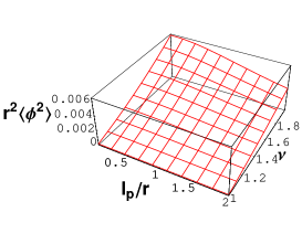
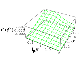
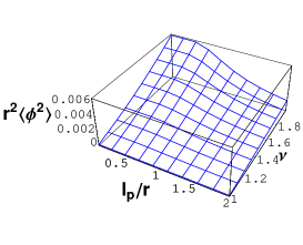
(P)                                             (A)                                             (S)

Figure 4: $r^{2}\langle\phi^{2}\rangle$ is plotted against $l_{p}/r$ and $\nu$, for (P) Padmanabhan-type, (A) Abel-type, and (S) Siegel-type.

The quantum stress tensors can be obtained from the formula (44) with (45) and the Green’s functions in the previous subsection. We exhibit $r^{4}\langle T_{r}^{r}\rangle$ in Fig. 5, $r^{4}\langle T_{\tilde{\theta}}^{\tilde{\theta}}\rangle$ in Fig. 6, and $r^{4}\langle T_{z}^{z}\rangle$ in Fig. 7, with a common choice, $\xi=1/6$. As in the case of $r^{2}\langle\phi^{2}\rangle$, quantities of Abel-type seem to have a small rise in the absolute values around $l_{p}/r\sim 0.5$. Except for this feature, Abel-type quantities almost resemble Siegel-type quantities.

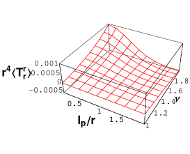
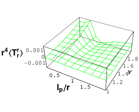
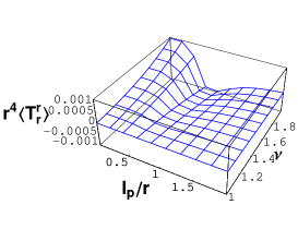
(P)                                             (A)                                             (S)

Figure 5: $r^{4}\langle T_{r}^{r}\rangle$ for $\xi=1/6$ is plotted against $l_{p}/r$ and $\nu$, for (P) Padmanabhan-type, (A) Abel-type, and (S) Siegel-type.

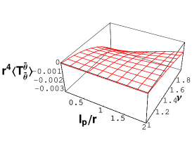
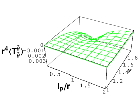
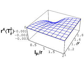
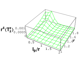
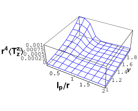
(P)                                             (A)                                             (S)

Figure 6: $r^{4}\langle T_{\tilde{\theta}}^{\tilde{\theta}}\rangle$ for $\xi=1/6$ is plotted against $l_{p}/r$ and $\nu$, for (P) Padmanabhan-type, (A) Abel-type, and (S) Siegel-type.

(P)                                             (A)                                             (S)

Figure 7: $r^{4}\langle T_{z}^{z}\rangle$ for $\xi=1/6$ is plotted against $l_{p}/r$ and $\nu$, for (P) Padmanabhan-type, (A) Abel-type, and (S) Siegel-type.

The trace of the quantum stress tensor does not vanish for finite $l_{p}$ even if $\xi=1/6$ in each case. Fig. 8 shows $r^{4}\langle T_{\lambda}^{\lambda}\rangle$ for $\xi=1/6$ in each case. We find, of course, $r^{4}\langle T_{\lambda}^{\lambda}\rangle=0$ if $l_{p}=0$ in each case.

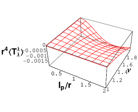
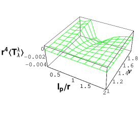
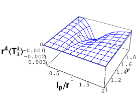
(P)                                             (A)                                             (S)

Figure 8: $r^{4}\langle T_{\lambda}^{\lambda}\rangle$ for $\xi=1/6$ is plotted against $l_{p}/r$ and $\nu$, for (P) Padmanabhan-type, (A) Abel-type, and (S) Siegel-type.

Inclusion of $l_{p}$ tinily violates conservation law $\nabla_{\lambda}\langle T_{\sigma}^{\lambda}\rangle=0$. Fig. 9 shows $r^{5}\nabla_{\lambda}\langle T_{r}^{\lambda}\rangle$ for $\xi=1/6$ in each case. We naturally find that this value vanishes in each case if $l_{p}=0$.

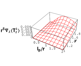
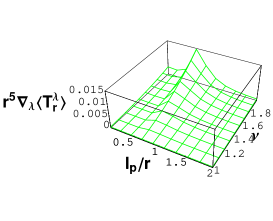
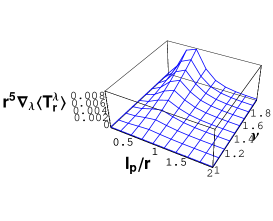
(P)                                             (A)                                             (S)

Figure 9: $r^{5}\nabla_{\lambda}\langle T_{\lambda}^{\lambda}\rangle$ for $\xi=1/6$ is plotted against $l_{p}/r$ and $\nu$, for (P) Padmanabhan-type, (A) Abel-type, and (S) Siegel-type.

IV.3 The expectation values in the neighborhood of the origin $r=0$

In this subsection, we would like to investigate the values of $\langle\phi^{2}\rangle$ and $\langle T_{\sigma}^{\rho}\rangle$ in three UV improved schemes near and at the origin $r=0$, where a conical singularity is located. Recall that, in the standard scheme without fundamental length, they behave $\langle\phi^{2}\rangle\propto 1/r^{2}$ and $\langle T_{\sigma}^{\rho}\rangle\propto 1/r^{4}$ in four dimensions, thus the values of them diverge at the origin.

In Fig. 10, the values of $l_{p}^{2}\langle\phi^{2}\rangle$ are plotted against $r/l_{p}$ and $\nu$ for three cases of Green’s functions. We find that $\langle\phi^{2}\rangle$ is finite at $r=0$ and a monotonic function of both $r$ and $\nu$ for each type.

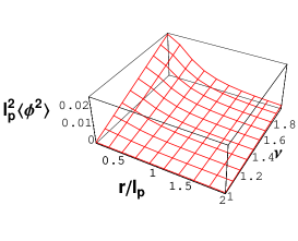
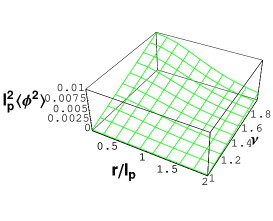
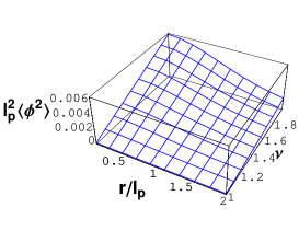
(P)                                             (A)                                             (S)

Figure 10: $l_{p}^{2}\langle\phi^{2}\rangle$ is plotted against $r/l_{p}$ and $\nu$, for (P) Padmanabhan-type, (A) Abel-type, and (S) Siegel-type.

The limiting value $\langle\phi^{2}\rangle(0)$ can be obtained in a rigorous form for each type, even in general dimensions. To this end, we remark, from (40),

$$\bar{K}_{D,\nu}(0,0;s)={\textstyle\frac{1}{2\pi(4\pi s)^{D/2}}}\int_{0}^{\infty}\left[{\textstyle-\frac{2\nu\sin\nu\pi}{\cosh\nu v-\cos\nu\pi}}\right]dv=\frac{\nu-1}{(4\pi s)^{D/2}}=(\nu-1)K_{D}(0,0;s)\,,$$ (64)

and we find

$$\langle\phi^{2}\rangle^{(*)}(0)=(\nu-1)G_{D}^{(*)}(0,0)\qquad({\textstyle(*)=(P),(A),\mbox{~{}and~{}}(S)})\,.$$ (65)

Here, we should recall that $G_{D}^{(*)}(x,x^{\prime})$ is the Green’s function in the space without singularity. According to (15), the values for $D=4$ are found to be

$$G_{4}^{(P)}(0,0)=\frac{1}{4\pi^{2}l_{p}^{2}}\,,\quad G_{4}^{(A)}(0,0)=\frac{1}{32\pi l_{p}^{2}}\,,\quad G_{4}^{(S)}(0,0)=\frac{1}{16\pi^{2}l_{p}^{2}}\,.$$ (66)

Therefore, the value of vacuum fluctuation from Padmanabhan-type Green’s function in four dimensions can be confirmed at the special point $r=0$ by using (49) with (50).

The stress tensors near the origin are shown in Figs. 11–14. We exhibit $l_{p}^{4}\langle T_{r}^{r}\rangle$ in Fig. 11, $l_{p}^{4}\langle T_{\tilde{\theta}}^{\tilde{\theta}}\rangle$ in Fig. 12, $l_{p}^{4}\langle T_{z}^{z}\rangle$ in Fig. 13, and $l_{p}^{4}\langle T_{\lambda}^{\lambda}\rangle$ in Fig. 14, with a common choice, $\xi=1/6$.

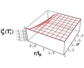
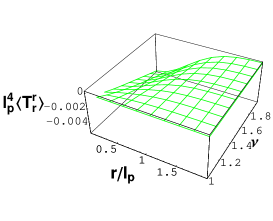
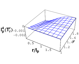
(P)                                             (A)                                             (S)

Figure 11: $l_{p}^{4}\langle T_{r}^{r}\rangle$ for $\xi=1/6$ is plotted against $r/l_{p}$ and $\nu$, for (P) Padmanabhan-type, (A) Abel-type, and (S) Siegel-type.

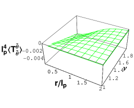
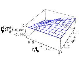
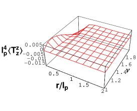
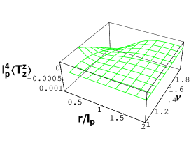
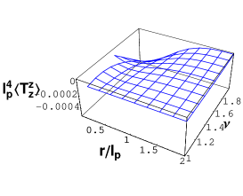
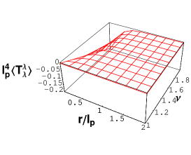
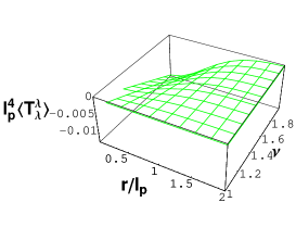
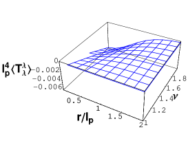
(P)                                             (A)                                             (S)

Figure 12: $l_{p}^{4}\langle T_{\tilde{\theta}}^{\tilde{\theta}}\rangle$ for $\xi=1/6$ is plotted against $r/l_{p}$ and $\nu$, for (P) Padmanabhan-type, (A) Abel-type, and (S) Siegel-type.

(P)                                             (A)                                             (S)

Figure 13: $l_{p}^{4}\langle T_{z}^{z}\rangle$ for $\xi=1/6$ is plotted against $r/l_{p}$ and $\nu$, for (P) Padmanabhan-type, (A) Abel-type, and (S) Siegel-type.

(P)                                             (A)                                             (S)

Figure 14: $l_{p}^{4}\langle T_{\lambda}^{\lambda}\rangle$ for $\xi=1/6$ is plotted against $r/l_{p}$ and $\nu$, for (P) Padmanabhan-type, (A) Abel-type, and (S) Siegel-type.

The values of $\langle T^{\rho}_{\sigma}\rangle^{(*)}(0)$ are also analytically expressed, similarly to the case with the values of $\langle\phi^{2}\rangle(0)$, containing $G_{D+2}^{(*)}(0,0)$ in the present case, however. That is:

$$\langle T^{r}_{r}\rangle^{(*)}(0) = \langle T^{\tilde{\theta}}_{\tilde{\theta}}\rangle^{(*)}(0)=-4\pi G_{D+2}^{(*)}(0,0)\left[{\textstyle\frac{(D-2)[D(\nu-1)+1]}{4(D-1)}+\nu\left(\xi-\frac{D-2}{4(D-1)}\right)}\right]\,,$$ (67)

$$\langle T^{z}_{z}\rangle^{(*)}(0) = -4\pi G_{D+2}^{(*)}(0,0)\left[{\textstyle\frac{D(D-3)(\nu-1)-2}{4(D-1)}+2\nu\left(\xi-\frac{D-2}{4(D-1)}\right)}\right]\,,$$ (68)

$$\langle T^{\lambda}_{\lambda}\rangle^{(*)}(0) = -4\pi G_{D+2}^{(*)}(0,0)\left[{\textstyle\frac{D(D-2)(\nu-1)}{4(D-1)}+2(D-1)\nu\left(\xi-\frac{D-2}{4(D-1)}\right)}\right]\,,$$ (69)

where the choice $\xi=\frac{D-2}{4(D-1)}$ is called the conformal coupling in $D$ dimensions. Incidentally, the values of the coincidence limit of $G_{D+2}^{(*)}(0,0)$ for $D=4$ are found to be

$$G_{6}^{(P)}(0,0)=\frac{1}{4\pi^{3}l_{p}^{4}}\,,\quad G_{6}^{(A)}(0,0)=\frac{1}{64\pi^{3}l_{p}^{4}}\,,\quad G_{6}^{(S)}(0,0)=\frac{1}{128\pi^{3}l_{p}^{4}}\,.$$ (70)

It is interesting to point out that there is the relevance to the Green’s function in “other dimensions” and it reminds us of discussion in Ref. CFI .

We find that quantum stress tensors $\langle T^{\rho}_{\sigma}\rangle$ are finite even if $\nu=1$. Although the origin of this “anomaly” has not been elucidated yet, this will be discussed later in Sec. V.

Finally, we show $l_{p}^{5}\nabla_{\lambda}\langle T_{r}^{\lambda}\rangle$ in Fig. 15 in each case. This value is non-zero near the conical singularity but rapidly falls off to zero at $r\gg l_{p}$ in each case.

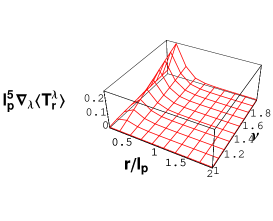
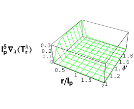
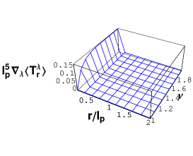
(P)                                             (A)                                             (S)

Figure 15: $l_{p}^{5}\nabla_{\lambda}\langle T_{r}^{\lambda}\rangle$ for $\xi=1/6$ is plotted against $r/l_{p}$ and $\nu$, for (P) Padmanabhan-type, (A) Abel-type, and (S) Siegel-type.

V Conclusion

We have presented the vacuum expectation values for a massless scalar field obtained from three types of the UV improved Green’s functions in non-simply connected spaces. Although the behavior of these values in a various range of scale is almost common, the quantities calculated from Abel-type Green’s function show a minute behavior if the typical scale of the system is close to the Planck scale, i.e., the cutoff scale. Interestingly, the present results should be directly relevant to the study of the Unruh effect Unruh ; Takagi ; Dowker and the quantum inconsistency of the space with closed timelike curves Hawking .

The UV improved Green’s functions we examined in this paper are mathematically simple ones, where the Planck length is introduced “by hand”, though certain physical motivation exists for each type of UV modification. Through the present study, however, it is revealed that the quantum quantities have slightly different behaviors around the small scale according to the type of UV completion. These results would be useful when we pursue the fundamental origin of UV completion and when we consider the back-reaction of quantum effects to space(time) structure. In any case, the mechanism of UV completion will require further investigation.

The “anomaly” encountered in the quantum stress tensors just at the conical singularity should be investigated further. This should be linked to the prescription of “refinement” or “renormalization” of the quantum quantities. The finite but comparatively large values of order $l_{p}^{-n}$ ($n$ is a positive integer) in quantum corrections have not ever been observed and should not directly affect known physical consequence. Anyway, the “renormalization” such as $\overline{\langle T_{\rho\sigma}\rangle}=\langle T_{\rho\sigma}\rangle-\lim_{\nu\rightarrow 1}\langle T_{\rho\sigma}\rangle$ can also be allowed, so we think that it would be necessary to study the connection between the renormalization and the back-reaction problem, where we should reconsider coupling to space(time) geometry.

Generalizing to other situations should also be possible. We have restricted our attention to the massless scalar case in this paper. The extension of the present analyses to massive cases should be straightforward, at least for the models of Padmanabhan-type and Siegel-type. It would be interesting to generalize our study to calculations in curved spaces or near black holes, including scattering problems with UV completion. Although the general treatment of the curved background might be hard, we may start with adopting a perturvative expansion around a trivial space.

Alternatively, the most direct generalization is considering constant-curvature background spaces, such as $S^{N}$ corresponding to Euclidean de Sitter space and $H^{N}$ corresponding to Euclidean anti-de Sitter space. The standard heat kernel in such spaces are already known (see, for example, Ref. Camporesi ). Accordingly, the quantum effects around BTZ black holes Steif ; LO ; SM1 ; SM2 with UV completion are within the scope of feasible study in near future.

We consider that mathematical properties of Green’s functions and heat kernels with the cutoff scale is also an interesting subject to study. We have already seen that the conservation law and the conformal symmetry are violated and broken by introducing the Planck length in three cases studied in this paper. In an academic point of view, we should study where, when, and how such fundamental law and symmetry can be protected in more general way of UV completion with close inspection. That is to say, we should take corrections in the definition of the stress tensor and field equations into account. In addition, we intend to investigate the mathematical nature of the heat kernel in the UV completion schemes. For example, we notice the fact that the standard heat kernel without cutoff scale in a direct-product space is the product of the heat kernels associated to two spaces. The fundamental “rule” in this level may yield a new guideline in theoretical research of physical contribution from very small scale physics.

Appendix A definitions of special functions and their properties

Almost all definitions and properties of the special functions exhibited below can be found in Ref. GR .

A.1 Modified Bessel function of the first kind

$$I_{\nu}(z) = \frac{2(z/2)^{\nu}}{\sqrt{\pi}\,\Gamma({\textstyle\nu+\frac{1}{2}})}\int_{0}^{\pi/2}\cosh(z\cos\theta)\sin^{2\nu}\theta d\theta$$ (71)

$$= \frac{1}{2\pi}\int_{-\pi}^{\pi}e^{z\cos\theta}\cos\nu\theta\,d\theta-\frac{\sin\nu\pi}{\pi}\int_{0}^{\infty}e^{-z\cosh v-\nu v}\,dv\,.$$

The integral formula

$$\int_{0}^{\infty}e^{-px}I_{\nu}(cx)dx=\frac{c^{\nu}}{\sqrt{p^{2}-c^{2}}(p+\sqrt{p^{2}-c^{2}})^{\nu}}$$ (72)

leads to (46) from (36).

A.2 Modified Struve function

$$\mathbf{L}_{\nu}(z)=\frac{2(z/2)^{\nu}}{\sqrt{\pi}\,\Gamma({\textstyle\nu+\frac{1}{2}})}\int_{0}^{\pi/2}\sinh(z\cos\theta)\sin^{2\nu}\theta d\theta\,.$$ (73)

A.3 Jacobi’s theta function

$$\vartheta_{3}(v,\tau)=1+2\sum_{n=1}^{\infty}e^{\tau\pi in^{2}}\cos(2n\pi v)=e^{\pi i/4}\tau^{-1/2}e^{-\pi iv^{2}/\tau}\vartheta_{3}(v/\tau,-1/\tau)\,.$$ (74)

Consequently, one can find

$$\sum_{n=-\infty}^{\infty}e^{-4\pi^{2}(n+\delta)^{2}s/L^{2}}e^{2\pi i(n+\delta)y/L}=\frac{L}{\sqrt{4\pi s}}\sum_{n=-\infty}^{\infty}e^{-(y-nL)^{2}/(4s)+2\pi\delta in}\,.$$ (75)

A.4 Modified Bessel function of the second kind

$$K_{\nu}(z) = K_{-\nu}(z)=\frac{1}{2}\left(\frac{z}{2}\right)^{\nu}\int_{0}^{\infty}\exp\left[-t-\frac{z^{2}}{4t}\right]t^{-\nu-1}dt$$ (76)

$$= \frac{1}{2}\int_{-\infty}^{\infty}\exp\left[-\nu t-z\cosh t\right]dt=\int_{0}^{\infty}\exp\left[-z\cosh t\right]\cosh\nu t\,dt\,.$$

$$K_{\nu}(z)\sim\frac{2^{\nu-1}\Gamma(\nu)}{z^{\nu}}\quad z\rightarrow 0\,,\qquad K_{\nu}(z)\sim\sqrt{\frac{\pi}{2z}}e^{-z}\quad z\rightarrow\infty\,.$$ (77)

A.5 Summation formulas

$$\sum_{n=1}^{\infty}\frac{\cos(n\delta)}{n^{2}+a^{2}}=\frac{\pi}{2a}\frac{\cosh[a(\pi-\delta)]}{\sinh(a\pi)}-\frac{1}{2a^{2}}\,.$$ (78)

$$\sum_{n=1}^{\infty}\frac{\cos(n\delta)}{(n^{2}+a^{2})^{2}}=-\frac{1}{2a^{4}}+\frac{\pi}{4a^{3}}\frac{\cosh[a(\pi-\delta)]+a\delta\sinh[a(\pi-\delta)]}{\sinh(a\pi)}+\frac{\pi^{2}}{4a^{2}}\frac{\cosh(a\delta)}{\sinh^{2}(a\pi)}\,.$$ (79)

Appendix B integration formulas

The formulas below have been used in calculations of quantum expectation values in the limit $r\rightarrow 0$ in Sec. IV.

$$\int_{0}^{\infty}\frac{-2\nu\sin\nu\pi}{\cosh\nu v-\cos\nu\pi}dv=2\pi(\nu-1)\quad(\nu>1)\,,$$ (80)

$$\int_{0}^{\infty}\frac{-2\nu\sin\nu\pi}{\cosh\nu v-\cos\nu\pi}\cosh v\,dv=2\pi\quad(\nu>1)\,,$$ (81)

$$\int_{0}^{\infty}\frac{\nu^{3}\sin\nu\pi(-3+2\cos\nu\pi\cosh\nu v+\cosh 2\nu v)}{(\cosh\nu v-\cos\nu\pi)^{3}}dv=0\quad(\nu>1)\,,$$ (82)

$$\int_{0}^{\infty}\frac{\nu^{3}\sin\nu\pi(-3+2\cos\nu\pi\cosh\nu v+\cosh 2\nu v)}{(\cosh\nu v-\cos\nu\pi)^{3}}\cosh v\,dv=2\pi\quad(\nu>1)\,.$$ (83)

References

(1)
T. Padmanabhan,
“Duality and zero-point length of spacetime”,
Phys. Rev. Lett. 78 (1997) 1854.
hep-th/9608182.
(2)
T. Padmanabhan,
“Hypothesis of path integral duality. I. quantum gravitational corrections to
the propagator”,
Phys. Rev. D57 (1998) 6206.
(3)
T. Padmanabhan,
“Principle of equivalence at Planck scales, QG in locally inertial frames and
the zero-point-length of spacetime”,
Gen. Rel. Grav. 52 (2020) 90.
arXiv:2005.09677 [gr-qc].
(4)
T. Padmanabhan,
“Probing the Planck scale: The modification of the time evolution operator due to
the quantum structure of spacetime”,
JHEP 2011 (2020) 013.
arXiv:2006.06701 [gr-qc].
(5)
T. Padmanabhan,
“Planck length: Lost+found”,
Phys. Lett. B809 (2020) 135774.
(6)
T. Padmanabhan,
“A class of QFTs with higher derivative field equations leading to standard
dispersion relation for the particle excitations”,
Phys. Lett. B811 (2020) 135912.
arXiv:2011.04411 [hep-th].
(7)
K. Srinivasan, L. Sriramkumar and T. Padmanabhan,
“Hypothesis of path integral duality. II. corrections to
quantum field theoretic result”,
Phys. Rev. D58 (1998) 044009.
gr-qc/9710104.
(8)
D. Kothawala, L. Sriramkumar, S. Shankaranarayanan and T. Padmanabhan,
“Path integral duality modified propagators in spacetimes with constant
curvature”,
Phys. Rev. D80 (2009) 044005.
arXiv:0904.3217 [hep-th].
(9)
S. Abel and N. Dondi,
“UV completion on the worldline”,
JHEP 1907 (2019) 090.
arXiv:1905.04258 [hep-th].
(10)
S. Abel, L. Buoninfante and A. Mazumdar,
“Nonlocal gravity with worldline inversion symmetry”,
JHEP 2001 (2020) 003.
arXiv:1911.06697 [hep-th].
(11)
W. Siegel,
“String gravity at short distances”,
hep-th/0309093.
(12)
L. Buoninfante, G. Lambiase and A. Mazumdar,
“Ghost-free infinite derivative quantum field theory”,
Nucl. Phys. B944 (2019) 114646.
arXiv:1805.03559 [hep-th].
(13)
D. V. Vassilevich,
“Heat kernel expansion: user’s manual”,
Phys. Rep. 388 (2003) 279.
(14)
R. Camporesi,
“Harmonic analysis and propagators on homogeneous spaces”,
Phys. Rep. 196 (1990) 1.
(15)
P. Candelas and S. Weinberg,
“Calculation of gauge couplings and compact circumferences from self-consistent
dimensional reduction”,
Nucl. Phys. B237 (1984) 397.
(16)
Y. Hosotani,
“Dynamical mass generation by compact extra dimensions”,
Phys. Lett. B126 (1983) 309.
(17)
N. Arkani-Hamed, H.-C. Cheng, P. Creminelli and L. Randall,
“Extranatural inflation”,
Phys. Rev. Lett. 90 (2003) 221302.
hep-th/0301218.
(18)
T. Inami, Y. Koyama, C. S. Lim and S. Minakami,
“Higgs inflation potential in higher-dimensional SUSY gauge theories”,
Prog. Theor. Phys. 122 (2009) 543. arXiv:0903.3637 [hep-th].
(19) A. Vilenkin,
“Cosmic strings and domain walls”,
Phys. Rep. 121 (1985) 263.
(20) G. Cognola, K. Kirsten and L. Vanzo,
“Free and self-interacting scalar fields in the presence of conical
singularities”,
Phys. Rev. D49 (1994) 1029. hep-th/9308106.
(21)
E. S. Moreira Jnr.,
“Massive quantum fields in a conical background”,
Nucl. Phys. B451 (1995) 365. hep-th/9502016.
(22) B. Linet,
“Quantum field theory in the space-time of a cosmic string”,
Phys. Rev. D35 (1987) 536.
(23) V. P. Frolov and E. M. Serebriany,
“Vacuum polarization in the gravitational field of a cosmic string”,
Phys. Rev. D35 (1987) 3779.
(24) A. G. Smith, The Formation and Evolution of Cosmic
Strings ed G. Gibbons, S. Hawking and T. Vachaspati (Cambridge:
Cambridge University Press, 1989) p. 263.
(25) K. Shiraishi and S. Hirenzaki,
“Quantum aspects of self-interacting fields around cosmic strings”,
Class. Quant. Grav. 9 (1992) 2277. arXiv:1812.01763 [hep-th].
(26)
E. Curiel, F. Finster and J. M. Isidro,
“Summing over spacetime dimensions in quantum gravity”,
Symmetry 12 (2020) 138.
arXiv:1910.11209 [gr-qc].
(27)
W. G. Unruh,
“Notes on black-hole evaporation”,
Phys. Rev. D14 (1976) 3357.
(28)
S. Takagi,
“Vacuum noise and stress induced by uniform acceleration”,
Prog. Theor. Phys. Suppl. 88 (1986) 1.
(29)
J. S. Dowker,
“Vacuum averages for arbitrary spin around a cosmic string”,
Phys. Rev. D36 (1987) 3742.
(30)
S. W. Hawking,
“Chronology protection conjecture”,
Phys. Rev. D46 (1992) 603.
(31) A. R. Steif,