Identifying and Addressing Nonstationary LISA Noise

Abstract

We anticipate noise from the Laser Interferometer Space Antenna (LISA) will exhibit nonstationarities throughout the duration of its mission due to factors such as antenna repointing, cyclostationarities from spacecraft motion, and glitches as highlighted by LISA Pathfinder. In this paper, we use a surrogate data approach to test the stationarity of a time series which does not rely on the Gaussianity assumption. The main goal is to identify noise nonstationarities in the future LISA mission. This will be necessary for determining how often the LISA noise power spectral density (PSD) will need to be updated for parameter estimation routines. We conduct a thorough simulation study illustrating the power/size of various versions of the hypothesis tests, and then apply these approaches to differential acceleration measurements from LISA Pathfinder. We also develop a data analysis strategy for addressing nonstationarities in the LISA PSD, where we update the noise PSD over time, while simultaneously conducting parameter estimation, with a focus on planned data gaps.

I Introduction

The Laser Interferometer Space Antenna (LISA) is a planned space-based gravitational wave (GW) mission with an expected launch in 2034 led by the European Space Agency (ESA) (Amaro-Seoane et al, 2017). The aim of this mission is to observe GW signals in the millihertz band which among others include astrophysical objects such as galactic white dwarf binaries (Carré and Porter, 2010), massive and supermassive black hole binaries (Sesana et al, 2005), and extreme mass ratio inspirals (EMRIs) (Chua et al, 2017). LISA will consist of a set of three spacecrafts arranged into an “equilateral” triangle, each separated by $L=2.5\times 10^{6}~{}\mathrm{km}$, connected with a laser link. The LISA constellation will cartwheel in an Earth-trailing heliocentric orbit around the Sun at an angle of 20 degrees between the Sun and Earth.

We expect LISA noise will be nonstationary in numerous ways. For example, as the spacecrafts will not always be able to point in the same direction towards Earth for us to receive data, there will be planned communication interruptions (or gaps), where the antennae will be repointed to adjust the beam (Carré and Porter, 2010; Baghi et al, 2019). This means physically moving the antennae, which will create noise. Another subtle effect of the repointing is that the distribution of mass near the test mass will change, which might affect the gravity gradient noise, leading to a change in acceleration noise (Purdue and Larson, 2007; Armano et al, 2019c). Controls may need to actively hold the proof mass using electrostatic actuation, which may lead to charging of the proof mass, and a change in the state of the noise (Baker et al, 2019; Pollack et al, 2010; Armano et al, 2019b).

Cyclostationarities are also expected in LISA, for example, due to the cartwheeling motion and orbits of the satellites. As LISA does not have uniform sensitivity in the sky and is more sensitive in the direction perpendicular to the plane of the constellation, there will be higher amplitude confusion noise when pointing to the line of sight of the galactic centre as this is where a large amount of galactic white dwarf binaries are located (Lamberts et al, 2019). In addition, LISA has a periodic orbit around the Sun, and pseudo-periodic solar activity can lead to cyclostationary noise (Adams and Cornish, 2010, 2014).

LISA Pathfinder (LPF) was an ESA satellite whose goal was to demonstrate the technology for the future LISA mission (Armano et al, 2016). Glitches in differential acceleration measurements $\Delta g$ have been analyzed in previous studies, occurring at a rate of one glitch per two days (Armano et al, 2016, 2018). As LISA will have a similar architecture to LPF, we expect glitches as another form of nonstationarity in the future mission (Robson and Cornish, 2019).

To understand exactly what it means to have nonstationary noise, first we must discuss precisely what a stationary process is. A (weakly) stationary time series $\mathbf{Y}=(Y_{1},Y_{2},\ldots,Y_{n})^{\top}$ is a stochastic process that has constant and finite mean and variance over time, i.e.,

$$\mathbb{E}[Y_{t}] = \mu<\infty,$$

$$\mathrm{Var}[Y_{t}] = \sigma^{2}<\infty,$$

for all $t$, and an autocovariance function $\gamma(.)$ that depends only on the time lag $s$ (Brockwell and Davis, 1991). That is, for a zero-mean weakly stationary process, the autocovariance function has the form

$$\gamma(s)=\mathbb{E}[Y_{t}Y_{t+s}],\quad\forall t,$$

where $\mathbb{E}[.]$ is the expected value operator, and $t$ represents time. Note that the PSD function is the Fourier transform of the autocovariance function.

Nonstationarities in a time series can therefore come in the form of a trend, heteroskedasticity, or time-varying autocorrelations (or PSDs). One can also consider amplitude modulation (AM) and frequency modulation (FM) to be forms of nonstationarity. In this paper, we are interested in a time-varying PSD structure, where we want to identify and handle this type of nonstationarity. To this end, we propose two hypothesis tests to identify whether a time series is stationary in terms of its PSD, which will be described in Sections II.3 and II.4. Further, we have developed an analysis strategy for dealing with nonstationary LISA noise, where we update the estimate of the noise PSD over time, rather than fixing it and assuming stationarity. It is worth noting that in the context of Laser Interferometer Gravitational-Wave Observatory (LIGO) data analysis, fluctuations in the PSD can bias parameter estimates (Aasi et al, 2013; Abbott et al, 2020; Biscoveanu et al, 2020a). Here, we are particularly interested in the gap problem (Carré and Porter, 2010; Baghi et al, 2019), where we believe satellite repointing could temporarily change the noise structure of the LISA satellites.

Common approaches to testing the stationarity of a time series are the so-called unit root tests, including the Augmented Dickey-Fuller (ADF) test (Said and Dickey, 1984), Phillips-Perron (PP) test (Phillips and Perron, 1988), and the Kwiatkowski-Phillips-Schmidt-Shin (KPSS) test (Kwiatkowski et al, 1992) for detecting a particular type of nonstationarity, namely a unit root autoregressive process. The behaviour of these unit root tests strongly depends on the long-run variance estimator used for rescaling the test statistic and they often fail to control the size, i.e. falsely reject stationarity too often for stationary time series with strong autocorrelation Müller (2005). Unit root tests have been noted in the GW literature by Romano and Cornish (2017) to not be of particular value as GW noise generally exhibits high autocorrelation with roots close to the unit circle. Moreover, these tests depend on the assumption of Gaussianity which may not be appropriate for GW data in the presence of glitches.

A purely visual test to check whether the periodograms change over time is based on the spectrogram by dividing the time series into smaller segments, and visualizing the successive segment-based periodograms. These form the starting point for formal spectral analysis tests that consider evolutionary (or time-varying) spectral estimates using time-frequency representations of the data. They share the common principle of comparing statistics based on adjacent segments. The most notable of these are the wavelet tests of von Sachs and Neumann (1998) and Nason et al (2000), where the authors propose using Haar wavelets of time-varying periodograms to test for covariance stationarity, and the Priestley-Subba Rao test (Priestley and Subba Rao, 1969) which tests the uniformity of a set of evolutionary spectra at different time intervals, and is similar to a two-factor analysis of variance (ANOVA). The wavelet test and Priestley-Subba Rao test use the asymptotic distribution of their test statistic under various assumptions on the local spectra which might be difficult to verify in any particular situation and often rely on Gaussian distributions, thus failing to control the size for heavy-tailed distributions. The Priestley-Subba Rao test requires the independence of time-frequency bins which may lead to stationarity decision errors due to biased estimations. In the context of GW data analysis for LIGO and Virgo, Abbott et al (2020) visualized potential nonstationarity of LIGO noise time series by a scalogram showing the amplitudes of wavelet basis functions at each discrete time and frequency. After prewhitening the data, the sum of squares of wavelet amplitudes would have a chi-squared distribution when applied to stationary Gaussian noise. Then, an Anderson-Darling test (Anderson and Darling, 1954) was applied to test against deviations from this chi-squared distribution. Its performance will depend critically on the assumption of Gaussianity and the spectral density estimate used for pre-whitening. Therefore, the development of stationarity tests against the alternative of a time-varying PSD that do not rely on Gaussian assumptions is important for practical analysis of GW data.

To avoid reliance on restrictive assumptions to derive the asymptotic distribution of the test statistic under the null hypothesis, various resampling approaches for testing the stationarity of a time series have also been introduced. One such approach by Swanepoel and Van Wyk (1986) uses a modification of the bootstrap of Efron (1979) to test the equality of two spectral densities from two independent time series. This approach still depends on parametric assumptions as autoregressive models are fitted to the data in each segment and the bootstrap is based on the independence assumption which is not given for overlapping segments. The test is applicable only for two independent time series and would suffer from the multiple comparison problem for multiple segments. Dette and Paparoditis (2007) use a frequency-domain bootstrap based on the $L_{2}$ between two nonparametrically estimated PSDs and pooled PSD. It does not make the assumption of independence but requires the estimation of the spectral density matrix which would only be possible with considerable computational time in the case of spectrograms. In general, the power of bootstrap tests for stationarity depends on the particular type of bootstrap and though asymptotically consistent under certain conditions, they do not provide general finite-sample guarantees (McCullough and Kareem, 2013).

To avoid deficiencies of the bootstrap methods, our tests fall into the lesser-known surrogate data tests which were first introduced by Theiler et al (1992) for testing non-linearities in time series, and later adapted by Xiao et al (2007) and Borgnat and Flandrin (2009) for testing stationarity. These tests are nonparametric in nature, where the original data are resampled to create stationary surrogates with the same periodogram. A version of the multitaper spectrogram of Thomson (1982) with Hermite (rather than Slepian) window functions (as discussed by Bayram and Baraniuk (2000)) is computed, where the estimated spectrum in each time segment is compared to a time-averaged spectrum using a distance measure, typically a combination of the Kullback-Leibler divergence and the log spectral deviation. The test statistic for these tests are the sample variance of these distances and a Gamma distribution is fitted to describe the null distribution of test statistics.

In this paper, we propose two variants on the surrogate data testing of Xiao et al (2007) and Borgnat and Flandrin (2009) that do not rely on the Gamma distributon to describe the distribution of the test statistic under the null hypothesis. We consider an autoregressive spectrogram where each short-time segment uses a frequentist autoregressive (AR) estimate of its spectrum, with order selected based on the Akaike information criterion (AIC). In the first variant, we can compute the Kolmogorov-Smirnov statistic, the Kullback-Leibler distance, or the log spectral distance to measure the distance between local spectra of short time segments and the global spectrum. A test statistic is then computed as the sample variance of these distances and we use surrogates to populate the sampling distribution of this test statistic under the null hypothesis of stationarity. Large variability in the distances of the original time series would provide evidence against stationarity. As a novel alternative, we fit a least squares regression line to the cumulative median of Euclidean distances between columns in the AR spectrogram. The slope of this line is used as a test statistic and surrogates are again used to generate the null distribution. Here, if a time series is stationary, we would expect the PSD in neighbouring segments of the spectrogram to be similar over time, meaning the median of Euclidean distances should fluctuate around a constant. A non-zero slope would then provide evidence against the stationarity hypothesis. In both variants, empirical percentiles are used to create a critical value that is used as a rejection threshold.

We introduce these hypothesis tests to be used as a tool for future LISA data analysis, with the overall goal of determining how often we should update the noise PSD. Once this is decided, parameter estimation routines can be implemented. In this paper, we propose the use of a blocked Metropolis-within-Gibbs sampler to simultaneously estimate the parameters of a galactic white-dwarf binary gravitational wave signal and estimating the noise PSDs before and after a planned data gap. We show that the stationarity tests based on the surrogate data approach can be applied to the residuals to check the validity of model assumptions.

The paper is structured as follows. In Section II, we introduce the notion of surrogate data testing, defining two specific hypothesis tests to be used in the future LISA mission. We then conduct a simulation study to demonstrate the power of these tests, and then apply the tests to differential acceleration measurements from LPF to highlight nonstationarities in that data. In Section III, we introduce our data analysis strategy for handling nonstationary LISA noise. We inject a galactic white-dwarf binary GW signal in piecewise stationary noise and implement a blocked Metropolis-within-Gibbs sampler for posterior computation of both signal parameters and noise PSDs. We mimic what we believe could happen to LISA noise when repointing satellites during planned gaps, and apply stationarity tests to residuals for model checking. We then give concluding remarks in Section IV.

II Identifying Nonstationary Noise

II.1 Stationary Surrogates

Surrogate data testing was originally proposed by Theiler et al (1992) for testing non-linearities in time series, and later adapted by Xiao et al (2007) and Borgnat and Flandrin (2009) for testing stationarity. The main idea here is that one can create stationary “surrogates” of a (potentially nonstationary) time series by directly manipulating the data in the frequency-domain, preserving the second-order statistics, but randomizing higher order statistics. In this way, we can generate a stationary surrogate of a time series that has the same empirical spectrum (periodogram) as the original time series.

First, Fourier transform the time series $Y(t),t=1,\ldots,n$ using

$$\tilde{Y}(\omega_{j})=\sum_{t=1}^{n}Y(t)\mathrm{e}^{-\mathrm{i}t\omega_{j}}$$

to get a frequency-domain representation where $\omega_{j}=2\pi j/n,j=0,\ldots,n-1$, are the Fourier frequencies. The Fourier coefficients can be expressed in polar coordinates such that

$$\tilde{Y}(\omega_{j})=A(\omega_{j})\mathrm{e}^{\mathrm{i}\varphi(\omega_{j})},$$

where $A(\omega_{j})=|\tilde{Y}(\omega_{j})|$ is the magnitude vector and $\varphi(\omega_{j})=\arg\left(\tilde{Y}\left(\omega_{j}\right)\right)$ is the phase vector.

Keeping the magnitude vector $(A(\omega_{0}),\ldots,A(\omega_{n-1}))$ fixed, we replace the phase vector $(\varphi(\omega_{1}),\ldots,\varphi(\omega_{n-1}))$ by a new phase vector $(\varphi^{*}(\omega_{1}),\ldots,\varphi^{*}(\omega_{n-1}))$ that is populated by iid $\mathrm{Uniform}[0,2\pi]$ random variables. We now have a randomized frequency-domain representation of the surrogate $\tilde{Y}^{*}(\omega_{j})=A(\omega_{j})\mathrm{e}^{\mathrm{i}\varphi^{*}(\omega_{j})}$ which is inverse Fourier transformed to give a time-domain representation of the surrogate:

$$Y^{*}(t)=\frac{1}{n}\sum_{j=0}^{n-1}\tilde{Y}^{*}(\omega_{j})\mathrm{e}^{\mathrm{i}t\omega_{j}}.$$

Assume $n$ is even and let $(\omega_{0},\omega_{1},\ldots,\omega_{n/2-1},\omega_{n/2})$ be the first Fourier frequencies. We only randomize the phase for $\omega_{1},\omega_{2},\ldots,\omega_{n/2-1}$ because $\omega_{0}$ and $\omega_{n/2}$ are always real-valued with zero phase, and the subsequent $n/2$ Fourier coefficients are complex conjugates of the first Fourier coefficients for the inverse Fourier transform to be real-valued, meaning $\varphi(\omega_{j})=-\varphi(\omega_{n-j})$.

Surrogates are extremely useful for testing stationarity as they not only have the same periodogram as the original data (which may or may not be stationary), but they are stationary themselves, meaning if one can compute a test statistic that can distinguish the null hypothesis (stationary) from the alternative hypothesis (nonstationary), it is straightforward to generate the sampling distribution of the test statistic by computing the test statistic on a large number of surrogates. We now focus our attention on useful test statistics based on the autoregressive spectrogram.

II.2 Autoregressive Spectrogram

The spectrogram is the most fundamental tool used in time-frequency analysis. It contains at each column an approximation of the PSD function for consecutive time intervals. Thus, it allows us to assess the evolution of this function over time. It is computed as follows. First compute the short-time Fourier transform (STFT),

$$\tilde{Y}(\omega,T)=\int W(t-T)Y(t)\mathrm{e}^{-\mathrm{i}t\omega}dt,$$

where $W(.)$ is a window function of duration $T$. Then take the squared modulus of each segment. This amounts to computing the periodogram of short windowed segments of the data, which may or may not be overlapping in time.

It is well-known in the time series literature that the periodogram is an asymptotically unbiased estimator of the spectral density function, but it is not a consistent estimator. This has lead to a large amount of literature on periodogram smoothing to reduce the variance.

The most popular parametric approach is to fit an autoregressive model where the order chosen by AIC. In this paper, we use an AR estimate of the spectrum for each segment of the spectrogram rather than using the raw periodogram. Although there are more sophisticated approaches to spectrum estimation that perhaps do not rely on parametric assumptions (see for example Choudhuri et al (2004), Edwards et al (2019), Kirch et al (2018), Maturana-Russel and Meyer (2019) for novel Bayesian approaches), we use the frequentist AR method for the sake of computational speed and ease.

For the remainder of the paper, when computing the AR spectrogram, we utilize the Tukey window with tapering coefficient equal to $(1-\mathrm{Overlap})/10$, where $\mathrm{Overlap}$ is the proportion of data that neighbouring time segments coincide.

II.3 Variance of Local Contrast (VOCAL) Test

In this section, we describe the first of two surrogate tests, which we call the Variance of Local Contrast (VOCAL) Test. As with any hypothesis test, we need to first define a test statistic that can distinguish between the null hypothesis and alternative hypothesis.

First consider the original time series and find its AR spectrogram. We need to contrast local features in the spectrogram with the global spectrum by computing a local contrast for each time segment (column) in the spectrogram. This is computed as

$$c_{l}=\kappa(\hat{f}_{l},\hat{f}),\quad l=1,2,\ldots,L,$$

where $L$ is the number of time segments (columns) in the spectrogram, $\hat{f}_{l}$ is the estimated (local) PSD of the $l^{\mathrm{th}}$ time segment of the spectrogram, $\hat{f}$ is the estimated (global) PSD of the entire time series (estimated using the same AR routine in the spectrogram), and $\kappa$ is a suitable spectral distance,

In this paper we use three different distance or dissimilarity measures $\kappa$ to specify the local contrasts. The first one uses the Kolmogorov-Smirnov (KS) statistic

$$\kappa^{(1)}(f_{1},f_{2})=\sup_{\omega}|F_{1}(\omega)-F_{2}(\omega)|,$$

where $F_{1}$ and $F_{2}$ are standardized empirical cumulative distribution functions (ECDFs) computed by normalizing the estimated PSDs $f_{1}$ and $f_{2}$ (such that they integrate to 1 and can be considered to be probability density functions), and taking their cumulative sums. The second one uses the symmetric Kullback-Leibler (KL) divergence

$$\kappa^{(2)}(f_{1},f_{2})=\frac{1}{2}\int\Big{(}f_{1}\left(\omega\right)-f_{2}\left(\omega\right)\Big{)}\log\frac{f_{1}(\omega)}{f_{2}(\omega)}\mathrm{d}\omega,$$

where $f_{1}$ and $f_{2}$ are normalized PSDs. The third is the log spectral distance (LSD), a dissimilarity measure defined directly on the unnormalized spectral densities by

$$\kappa^{(3)}(f_{1},f_{2})=\int\left|\log\frac{f_{1}(\omega)}{f_{2}(\omega)}\right|d\omega.$$

Whereas the KS and KL distance are insensitive to any changes in scale of the PSD because of the normalization, the LSD is well suited to quantify differences in both shape and scale such as amplitude modulations.

Fluctuations in the local contrasts can be used to distinguish between stationarity and nonstationarity as we would expect very little variability in the local contrasts if a time series was stationary and more variability if the time series was nonstationary. To this end, we use the sample variance of local contrasts as the test statistic for this test, i.e.,

$$V=\mathrm{Var}(\mathbf{c}),$$

where $\mathbf{c}=(c_{1},c_{2},\ldots,c_{L})$.

We can then generate the sampling distribution of this test statistic under the null hypothesis by repeating this same process on stationary surrogate data. That is, for each surrogate (indexed by $s=1,2,\ldots,S$, for large $S$) compute the AR spectrogram, the local contrasts $\mathbf{c}_{s}$, and finally the test statistic to give us

$$V_{0}(s)=\mathrm{Var}(\mathbf{c}_{s}),\quad s=1,2,\ldots,S,$$

where $\mathbf{c}_{s}=(c_{s,1},c_{s,2},\ldots,c_{s,L})$.

The hypothesis test can then be formalized by considering where $V$ lies in the distribution of $V_{0}$. Let

$$H_{0} : V<\gamma\quad\mathrm{(Stationary)},$$

$$H_{1} : V\geq\gamma\quad\mathrm{(Nonstationary)},$$

where $\gamma$ is the critical value chosen such that

$$p(V_{0}\leq\gamma)=1-\alpha,$$

where $\alpha$ is the rejection threshold. Thus for an $\alpha=0.05$ rejection threshold, $\gamma$ is computed as the 95% percentile of $V_{0}$. Alternatively, an approximate $p$-value can be computed by

$$\frac{1}{S}\sum_{s=1}^{S}I_{\{V_{0}(s)\geq V\}},$$

where $I$ is an indicator function. Note that this is a one-sided test.

The precision to which the $p$-value can be computed depends on the number of surrogates generated. For example, if $S=1,000$, the $p$-value can be computed to three decimal places, and if $S=10,000$, the $p$-value can be computed to four decimal places.

As an illustrative example of the test, consider the autoregressive (AR) model, defined as:

$$Y_{t}=\sum_{i=1}^{p}\varphi_{i}Y_{t-i}+\varepsilon_{t},$$

where $p$ is the order, $(\varphi_{1},\ldots,\varphi_{p})$ are the model parameters, and $\varepsilon_{t}\sim\mathrm{N}(0,\sigma^{2})$ for all $t$ is the white noise innovation process.

Consider the case where we have a length $n=2^{13}$ time series generated from an AR(2) with parameters (0.9, -0.9), and we concatenate this with a length $n=2^{13}$ time series generated from an AR(1) with parameter 0.9, each with standard normal innovations, as illustrated in Figure 1.

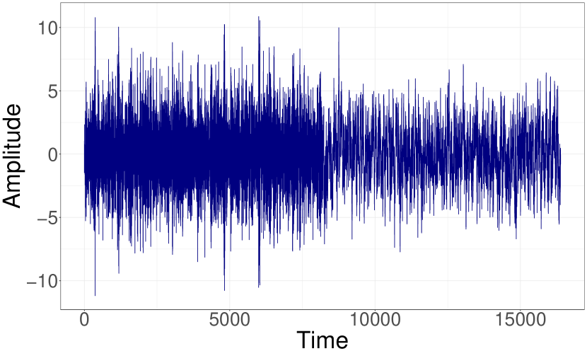
Figure 1: Time series containing $2^{13}$ realizations from an AR(2) with parameters $(0.9,-0.9)$ and $2^{13}$ realizations from an AR(1) with parameter 0.9. Each series uses N$(0,1)$ innovations.

Setting the overlap to 75% and window length to $2^{10}$, the associated AR spectrogram can be seen in Figure 2. Notice how the spectrum changes around halfway through the time series.

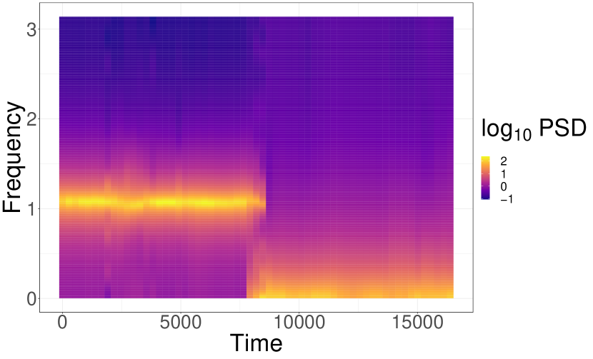
Figure 2: AR spectrogram from the time series presented in Figure 1. Notice the abrupt change in PSD structure at the halfway point.

We now generate 1,000 surrogates. One example of a surrogate of our original time series can be seen in Figure 3 and its associated AR spectrogram can be seen in Figure 4.

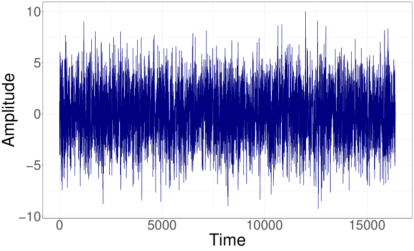
Figure 3: One example of stationary surrogate data based on the time series presented in Figure 1.

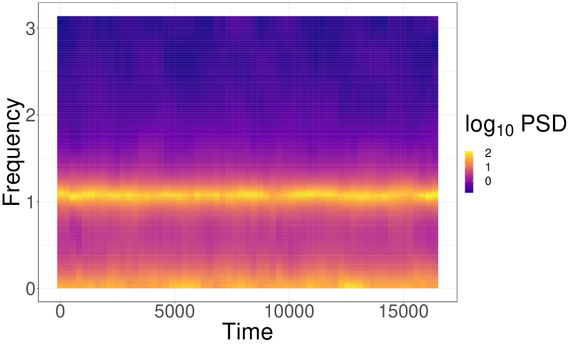
Figure 4: AR spectrogram from the stationary surrogate data presented in Figure 3.

Using the KS statistic as the local contrast, we can generate the test statistic $V$ from the original data, and the empirical sampling distribution of the test statistic using $(V_{0}(1),V_{0}(2),\ldots,V_{0}(S))$. Using a 5% rejection threshold, we compute the 95% percentile of the empirical sampling distribution. This is illustrated in Figure 5. As the test statistic $V$ is greater than the 95% percentile of the empirical sampling distribution, we reject the null hypothesis of stationarity.

Figure 5: Empirical sampling distribution of test statistic (variance of local contrasts computed using the KS statistic). The dotted black line is $\gamma$ (the 95% percentile of this null distribution) and the dashed pink line is the test statistic $V$ from the original time series.

II.4 Slope of Median Euclidean Distance (SOMED) Test

For our second surrogate test, we compare the Euclidean distances between the estimated PSD functions over time, i.e., a comparison between the columns of the spectrogram. If a time series is stationary, each column in the spectrogram should look approximately similar over time (see e.g., Figure 4). Consequently, a sequence of consecutive distances should fluctuate around a constant. We propose to test stationarity by testing the significance of the slope in a simple linear regression model fitted to these distances.

First, we calculate the AR spectrogram. This conforms a matrix $(r\times m)$ where the rows and columns stand for the energy or power at a particular frequency and the time intervals, respectively. Then, we calculate the Euclidean distance of each column with respect to the other ones, that is

$$d_{ij}=\sqrt{\sum_{k=1}^{r}\left(Y_{ki}-Y_{kj}\right)^{2}},$$

where $\textbf{Y}_{i}=(Y_{1i},\dots,Y_{ki},\dots,Y_{ri})^{\top}$ is the $i^{\text{th}}$ column of the spectrogram for $i=1,\dots,m$. The distances $d$ compound a symmetric matrix D which has a vector of zeros in its diagonal.

Since D is symmetric, we discard the upper triangular part and calculate the median of each row, which generates a sequence $\textbf{v}=(v_{2},\dots,v_{m})$, where $v_{i}$ is the median of the Euclidean distances of the estimated PSD for the $i^{\text{th}}$ time interval (column in the spectrogram matrix) with respect to all the estimated PSD of the previous time intervals, i.e., it is a cumulative median. Since the first $v_{i}$ values embody a few comparisons that tend to generate low discrepancies, these can be discarded, for instance, the first 10% of the sequence.

If the time series is stationary, we would expect a similar PSD across time. In other words, the cumulative median of the Euclidean distances should fluctuate around a constant, which can be tested evaluating the slope of a fitted simple linear regression model. Thus, we fit a linear model $y_{i}=\beta_{0}+\beta_{1}x_{i}+\varepsilon_{i}$, where the responses are the sequence v and the explanatory variables points in time. We assume that the errors $\varepsilon_{i}$ are independent and identically distributed with $\mathbb{E}(\varepsilon_{i})=0$ and $\text{Var}(\varepsilon_{i})=\sigma^{2}$. If the estimated slope is zero it means that the time series is stationary, otherwise the time series is nonstationary. We assess this assumption of the time series through the following hypotheses:

$$H_{0} :\beta_{1}=0\quad\text{(Stationary)}$$

$$H_{1} :\beta_{1}\neq 0\quad\text{(Nonstationary)}.$$

The null hypothesis establishes that the sequence of medians v does not change over time or equivalently the PSD functions do not vary significantly over time, showing the stationarity of the time series.

To test $H_{0}$, we compare the slope estimated from the original data $\widehat{\beta}$ with the empirical distribution of the slopes estimated from surrogate data sets $\mbox{\boldmath$\widehat{\beta}$}_{S}=(\widehat{\beta}_{1},\dots,\widehat{\beta}_{S})$, i.e., under the null hypothesis that assumes stationarity. Then, the $p$-value is calculated by

$$\dfrac{1}{S}\sum_{s=1}^{S}\left(I_{\left\{-\left|\widehat{\beta}\right|>\widehat{\beta}_{s}\right\}}+I_{\left\{\left|\widehat{\beta}\right|<\widehat{\beta}_{s}\right\}}\right),$$

where $I$ is an indicator function.

This test also has the potential of detecting glitches using conventional statistical techniques used to detect outliers in linear regression models. This can be assessed by analyzing the cumulative median values of the original data set.

Consider the AR spectrogram used in Section II.3. The nonstationary design of this process can be clearly noted in the spectrogram displayed in Figure 2. The two PSDs corresponding to the AR(2) and AR(1) processes have their peaks at different frequencies. This difference is also clear in the comparison of the Euclidean distances displayed in Figure 6. The discrepancy in the PSD estimates is represented in the magnitude of the distances which conform a block in the lower-right part.

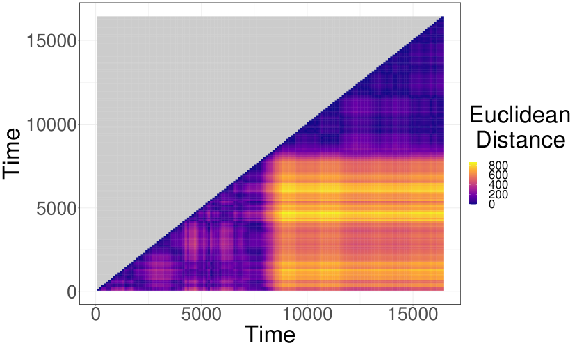
Figure 6: Euclidean distances for the spectrogram displayed in Figure 2.

The medians of the Euclidean distances of a specific time interval in Figure 6 with respect to its previous intervals are displayed in Figure 7. It can be noticed the design of the process: the first half is centred below the second one. The slope of the simple linear model is evidently non zero. The discrepancy of the PSD estimates do not seem to fluctuate randomly around a constant, which is evidence in favour of the nonstationary nature of the process. Comparing this slope with the empirical distribution of the slopes calculated from the surrogate data sets we get a $p$-value of 0.000. The SOMED test rejects the null hypothesis, identifying successfully this data set as nonstationary.

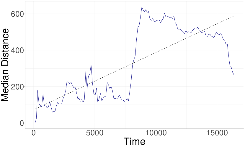
Figure 7: Median of the Euclidean distances for each column of Figure 6. The dashed line stands for a simple linear model.

II.5 Testing Simulated Data

We now apply the surrogate tests to simulated AR data (with standard white noise innovations) and compute power or size for different scenarios. Consider a length $n=2^{12}$ time series $\mathbf{Y}$ that is split in half into two length $n/2=2^{11}$ time series $\mathbf{Y}_{1}$ and $\mathbf{Y}_{2}$. For the following three scenarios, let $\mathbf{Y}_{1}$ and $\mathbf{Y}_{2}$ have the:

1. Same dependence structure;

2. Different dependence structure;

3. Similar dependence structure;

where “dependence structure” refers to the autocovariance function of a time series, or equivalently the spectral density function, which is its Fourier transform.

In Scenario 1, we consider a time series with the same dependence structure (and therefore same PSD) throughout its duration. Let $\mathbf{Y}_{1}$ and $\mathbf{Y}_{2}$ be generated from an AR(1) with parameter 0.9. In this scenario, we show that both tests yield small Type I Errors, i.e. do not reject the null hypothesis of stationarity the vast majority of times.

In Scenario 2, we look at an extreme example, where $\mathbf{Y}_{1}$ and $\mathbf{Y}_{2}$ have vastly different dependence structures. Let $\mathbf{Y}_{1}$ be generated from an AR(2) with parameters (0.9, -0.9) and $\mathbf{Y}_{2}$ be generated from an AR(1) with parameter 0.9. Here, we demonstrate that both methods reject the null hypothesis of stationarity, with high power.

In Scenario 3, we let $\mathbf{Y}_{1}$ and $\mathbf{Y}_{2}$ have very similar (but not equivalent) dependence structures. Let $\mathbf{Y}_{1}$ come from an AR(1) with parameter 0.8 and $\mathbf{Y}_{2}$ come from an AR(1) with parameter 0.9.

Finally we add a fourth scenario:

1. Time-varying dependence structure.

We use a time-varying autoregressive model (TVAR), where coefficients vary linearly from -0.6 to 0.6. Here, we demonstrate that both approaches reject the stationarity hypothesis when the spectrum is time-varying, with high power.

For each scenario we generate a time series, compute its AR spectrogram, and test statistic. We then create 1,000 stationary surrogates, compute their AR spectrograms and test statistics and compare the observed test statistic against the sampling distribution of test statistics. If the observed test statistic is in the tails of the distribution, this gives us evidence against the stationarity hypothesis. Specifically, we use the 95% percentile as the critical value for the one-sided VOCAL tests (i.e., a $p$-value of $<0.05$), and $p$-value of $<0.05$ for the two-sided SOMED test.

The AR spectrograms are generated using a window length of $T=2^{9}$, and overlap of 75%. We conduct both the VOCAL and the SOMED hypothesis tests, and consider the KS, KL, and LSD variants on the VOCAL test.

We replicate each simulation 1,000 times and report the size or power of each test, at the 5% significance level, where the size of a test is the probability of falsely rejecting the null hypothesis when it is true (or the probability of making a Type I Error), and the power of a test is the probability of correctly rejecting the null hypothesis when it is false (or one minus the probability of making a Type II Error). Type I and II Errors are equivalent to false positives and false negatives respectively. Our results are presented in Table 1.

Table 1: Test size (probability of falsely rejecting $H_{0}$ when it is true) for Scenario 1, and test power (probability of correctly rejecting $H_{0}$ when it is false) for Scenarios 2, 3, and 4.

Scenario	KS	KL	LSD	SOMED
1	0.036	0.048	0.046	0.046
2	1.000	1.000	1.000	1.000
3	0.794	0.739	0.049	0.962
4	1.000	1.000	1.000	0.999

We see that when $\mathbf{Y}_{1}$ and $\mathbf{Y}_{2}$ have the same PSD, all tests have a very small test size and that there is less than a 5% chance of making a Type I error. For the extreme case where $\mathbf{Y}_{1}$ and $\mathbf{Y}_{2}$ have very different PSDs, all tests give us power 1, which means there is zero chance of making a Type II error. In the case where we have similar but not equivalent PSDs, all tests reject the null hypothesis the majority of the time and the SOMED test works particularly well, which is remarkable considering how similar the $\mathbf{Y}_{1}$ and $\mathbf{Y}_{2}$ are. The LSD test, though, has very low power in this scenario, as it is less suited to discriminate between small changes in distributional shapes than the KL and KS distance measures. When we have a time-varying PSD, we again have high power. All of these results give us great confidence that the surrogate tests are performing as required.

II.6 LISA Pathfinder

We now demonstrate that our surrogate tests can detect nonstationarities in the clean (Level 3) $\Delta g$ data from the noise runs of LPF. These data have been corrected for the acceleration coming from centrifugal force, acceleration on the $x$-axis coming from the spacecraft motion along other degrees of freedom, and spurious acceleration noise from the digital to analog converter of the capacitive actuation and Euler force. Details can be found in the technical note on the LPF data archive (Armano et al, 2019a).

We analyze segments from two separate noise runs. These have the following starting times and lengths:

1. 2016-04-03 14:55:00 UTC for 12 days, 16 hours, 29 minutes, 59.40 seconds. We refer to this data set as the Glitch Data Set.

2. 2017-02-13 07:55:00 UTC for 18 days, 13 hours, 59 minutes, 59.40 seconds. We refer to this data set as the Amplitude Modulation (AM) Data Set.

The LPF data are originally sampled at a rate of 10 Hz (with sample interval $\Delta_{t}=0.1$ s). For the Glitch Data Set, we downsampled the data to 0.2 Hz ($\Delta_{t}=5$ s) to obtain a Nyquist frequency of 0.1 Hz (but first Tukey windowing with parameter 0.01, then applying a low-pass Butterworth filter of order 4 and critical frequency 0.1 Hz to avoid aliasing issues). The frequency range of interest for most GW signals detectable by LISA is $[10^{-4},10^{-1}]$ Hz. To resolve the lowest frequency in this band, the shortest (base 2) time series we can analyze is $n=2^{11}$. We therefore split the data into non-overlapping segments of length $n=2^{11}$ to speed up computations.

It is important to note that in the mean sense of stationarity, once filtered and downsampled, the Glitch Data Set is nonstationary, as there is a trend. We therefore remove this trend piecewise linearly for each non-overlapping segment, and we focus our attention on the question of whether LPF noise is nonstationary in terms of its autocovariance function, or equivalently its PSD. The AR spectrogram (with window length $T=2^{10}$ and 75% overlap) of the Glitch Data Set can be seen in Figure 8.

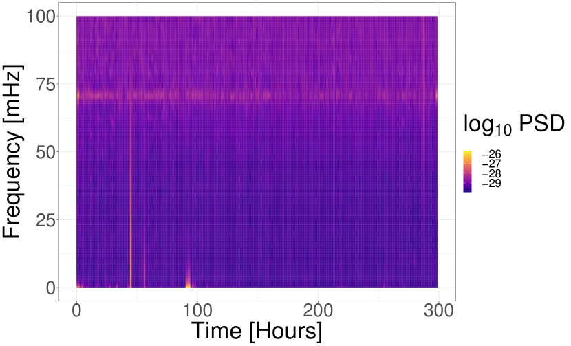
Figure 8: AR Spectrogram of the Glitch Data Set.

For the AM Data Set, we take the Level 3 data without any additional preprocessing. We examine the first four hours of this data set. The AR spectrogram (with window length $T=2^{10}$ and 75% overlap) of the AM Data Set can be seen in Figure 9.

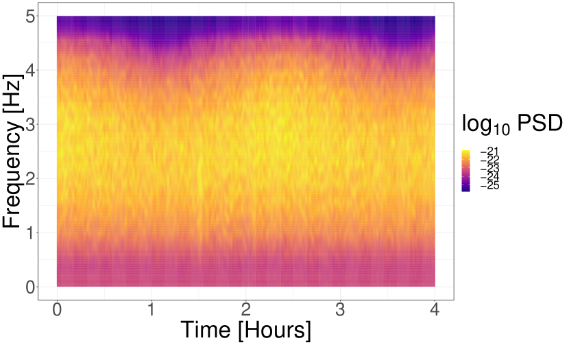
Figure 9: AR Spectrogram of the AM Data Set.

II.6.1 Glitch Data Set

Here, we analyze the Glitch Data Set for four different cases. These are:

1. The full time series (see Figure 10).

2. A segment with a large glitch at the end of the time series (see Figure 11).

3. A segment with a large glitch not at the end of the time series (see Figure 12).

4. A stationary segment with no glitches present (see Figure 13).

For the following surrogate tests, we compute an AR spectrogram with no overlap and window length $2^{9}$ for Case 1, and $2^{7}$ for Cases 2–4. 1,000 surrogates are then used to generate the sampling distribution of the test statistics.

The full downsampled, filtered, and piecewise linear detrended data can be seen in Figure 10. This data set is full of transient, high amplitude “glitches”.

Figure 10: $\Delta g$ LPF data from the Glitch Data Set.

When considering the full data set, we report a $p$-value of 0.001 for the KS variant and 0.000 for the KL and LSD variants of the VOCAL test, and 0.001 for the SOMED test. These results indicate that all of the surrogate tests provide evidence against the notion of stationarity, which we attribute to the glitches.

Now consider the case where we look at a segment of the data set where the largest glitch is present. We can see in Figure 10 that the largest glitch in the time series is somewhere around 45 hours into data collection (in the 15th segment from preprocessing). We zoom on this segment (of length $n=2^{11}$) and its neighbouring earlier (14th) segment in Figure 11.

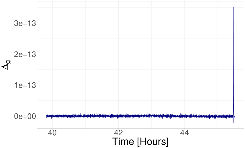
Figure 11: The 14th and 15th length $n=2^{11}$ segments from the Glitch Data Set. There is a noticeably large glitch at the end of the displayed time series.

When analyzing the time series in Figure 11, where the glitch is at the end of the time series, we report a $p$-value of 0.001 for the KS variant of the VOCAL test, 0.000 for the KL and LSD variants of the VOCAL test, and 0.002 for the SOMED test, all providing very strong evidence against the notion of stationarity. We attribute this nonstationarity to the glitch present in the data set.

The glitch at the end of the times series causes naturally a large Euclidean distance for the last interval in comparison to the previous ones in the SOMED test case. This is reflected in the estimated simple regression model. The glitch has a leverage effect in the estimated slope, which results in the rejection of the null hypothesis.

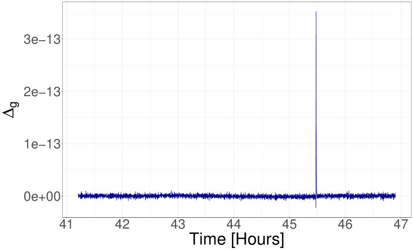
Figure 12: Same data as in Figure 11 but translated so that the glitch occurs 75% of the way through the time series.

When the large glitch is not at the end of the time series as in Figure 12, the KS, KL, and LSD variants of the VOCAL test all yield $p$-values of 0.000, meaning we have very strong evidence against stationarity. However, for the SOMED test, we report a $p$-value of 0.701, which means we are not rejecting the notion of stationarity here.

Unlike the previous case, the glitch is relatively in the middle of the sequence, which results in a large value in one of the central cumulative medians of the Euclidean distances in the SOMED test case. This large value has a null effect on the estimated slope of the linear model due to its position. Thus, the method fails wrongly to reject the null hypothesis. However, this large value can be visualized via the Cook’s distance, a measure of the impact of a single observation in the parameter estimates. In this case, the interval that contains the glitch has a Cook’s distance value of 0.39, which is extremely close to the cut point given by the rule of thumb 0.4, and it is quite different from the rest of the Cook’s distance values, which have a median of 0.014 and standard deviation of 0.070. Even though the SOMED test fails to reject the stationary hypothesis in this case, the glitch can be detected and thus the validity of the conclusions based on this test can be questioned. This procedure can be applied to other similar situations.

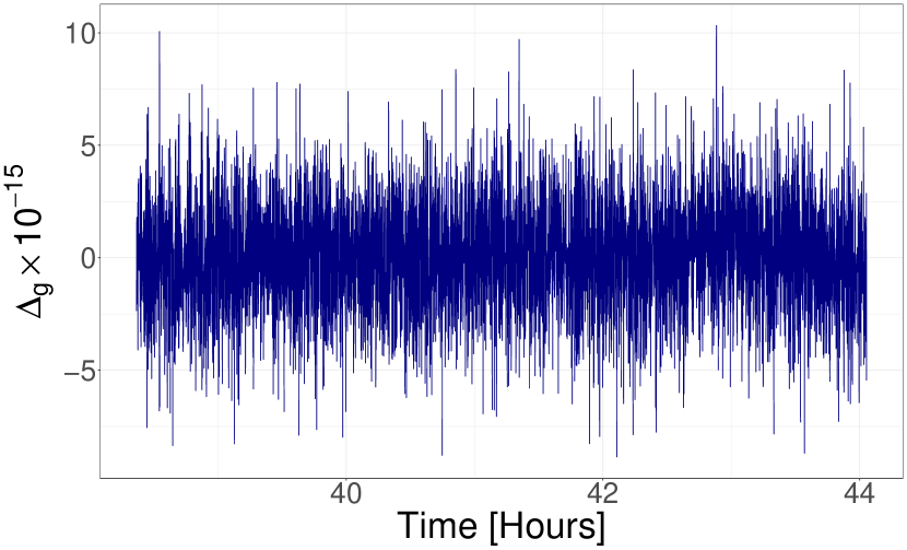
Figure 13: Stationary segment of the Glitch Data Set occurring before the large glitch in Figures 11 and 12.

For Case 4 where the data looks stationary, we report the following $p$-values: 0.836, 0.198, and 0.361 for the KS, KL, and LSD variants of the VOCAL test respectively, and 0.702 for the SOMED test. All three do not reject the null hypothesis, meaning we have no evidence against stationarity for this segment of data.

II.6.2 AM Data Set

We see cyclostationary behaviour in the LPF data. This is highlighted in the AM Data Set, which is illustrated in Figure 14.

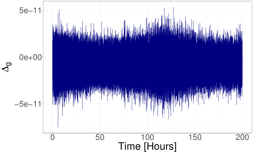
Figure 14: $\Delta g$ data from the AM Data Set.

For all of the surrogate tests, we compute an AR spectrogram with no overlap and window length $2^{9}$. Using 1,000 surrogates to generate the sampling distribution of the test statistics, we report a $p$-value of 0.008 for the KS variant of the VOCAL test, 0.000 for the KL and LSD variants of the VOCAL test, and 0.000 for the SOMED test, all providing very strong evidence against the notion of stationarity.

III Addressing Nonstationary Noise

Using the hypothesis tests defined in Section II.3 and Section II.4, or similar, we can identify if LISA noise is nonstationary. This will help us to determine where, and how often to split LISA data so that each time segment is locally stationary, with its own noise PSD (to be independently estimated/updated). Once we know where to segment the data, we can develop a LISA data analysis strategy.

Here we describe a parameter estimation routine for one non-chirping galactic binary GW signal, where we simultaneously estimate signal parameters and the LISA noise PSD over time to take into account the time-varying nature of the noise. We include a planned gap in the data stream and use different noise structures before and after the gap to mimic what we expect to happen to LISA noise due to antenna repointing.

III.1 Galactic White Dwarf Binary Gravitational Wave Signal Model

We assume the low frequency approximation to the LISA response as described by Carré and Porter (2010). We define the GW strain in one Time-Delay Interferometry (TDI) (Tinto and Dhurandhar, 2005) channel as

$$h(t)=h_{+}(t)F^{+}(t)+h_{\times}(t)F^{\times}(t),$$

where the GW polarisations are defined as

$$h_{+}(t) = A_{0}\left(1+\cos^{2}\iota\right)\cos\left(\Phi\left(t\right)+\varphi_{0}\right),$$

$$h_{\times}(t) = -2A_{0}\cos\iota\sin\left(\Phi\left(t\right)+\varphi_{0}\right),$$

for a non-chirping galactic white dwarf binary. Here, $A_{0}$ is the amplitude, $\iota$ is the inclination angle between the orbital plane of the source and the observer, $\varphi_{0}$ is the initial phase, and $\Phi(t)$ is the time-dependent phase, which for a circular orbit, is defined as

$$\Phi(t)=2\pi\omega_{0}\left(t+R_{\oplus}\sin\theta\cos\left(2\pi\omega_{m}t-\phi\right)\right),$$

where $\omega_{0}$ is the monochromatic frequency, $\omega_{m}$ is the LISA modulation frequency (defined as the reciprocal of the number of seconds in a year), $R_{\oplus}$ is the time light takes to travel one astronomical unit, and $(\theta,\phi)$ is the sky location of the source.

Using the definitions of Rubbo et al (2004), the antenna beam factors are

$$F^{+}(t) = \frac{1}{2}\left(\cos\left(2\psi\right)D^{+}\left(t\right)-\sin\left(2\psi\right)D^{\times}\left(t\right)\right),$$

$$F^{\times}(t) = \frac{1}{2}\left(\sin\left(2\psi\right)D^{+}\left(t\right)+\cos\left(2\psi\right)D^{\times}\left(t\right)\right),$$

where

$$\begin{split}D^{+}(t)&=\frac{\sqrt{3}}{64}\Bigg{(}-36\sin^{2}\left(\theta\right)\sin\left(2\alpha\left(t\right)-2\lambda\right)\\ &+\left(3+\cos\left(2\theta\right)\right)\bigg{(}\cos\left(2\phi\right)\Big{(}9\sin\left(2\lambda\right)\\ &-\sin\left(4\alpha\left(t\right)-2\lambda\right)\Big{)}+2\sin\left(2\phi\right)\\ &\Big{(}\cos\left(4\alpha\left(t\right)-2\lambda\right)-9\cos\left(2\lambda\right)\Big{)}\bigg{)}\\ &-4\sqrt{3}\sin\left(2\theta\right)\Big{(}\sin\left(3\alpha\left(t\right)-2\lambda-\phi\right)\\ &-3\sin\left(\alpha\left(t\right)-2\lambda+\phi\right)\Big{)}\Bigg{)},\\ D^{\times}(t)&=\frac{1}{16}\Bigg{(}\sqrt{3}\cos\left(\theta\right)\Big{(}9\cos\left(2\lambda-2\phi\right)\\ &-\cos\big{(}4\alpha\left(t\right)-2\lambda-2\phi\big{)}\Big{)}\\ &-6\sin\left(\theta\right)\Big{(}\cos\big{(}3\alpha\left(t\right)-2\lambda-\phi\big{)}\\ &+3\cos\big{(}\alpha\left(t\right)-2\lambda+\phi\big{)}\Big{)}\Bigg{)},\end{split}$$

and $\alpha(t)=2\pi\frac{t}{T}+\kappa$ is the orbital phase of the centre of mass of the constellation, where $T$ is the number of seconds in a year (though in this study, we increase the orbital modulation so that $T$ is the number of seconds in a day for computational reasons), and $\kappa=0$ is the initial ecliptic longitude.

The parameters we are interested in estimating are amplitude $A_{0}$, monochromatic frequency $\omega_{0}$, initial phase $\varphi_{0}$, and inclination $\iota$. All other parameters, e.g., sky location ($\theta,\phi$), GW polarization angle $\psi$, and initial ecliptic longitude $\kappa$, are fixed. To this end, we place the following noninformative priors on the signal parameters:

$$A_{0} \sim \mathrm{Uniform}[0,\infty),$$

$$\cos\varphi_{0} \sim \mathrm{Uniform}[-1,1],$$

$$\cos\iota \sim \mathrm{Uniform}[-1,1],$$

$$\omega_{0} \sim \mathrm{Uniform}[0.0001,0.0191].$$

Although data will eventually be analyzed in the three TDI channels A, E, and T (Tinto and Dhurandhar, 2005) (where T is the noise-only channel containing no signal information), for simplicity, we will only consider the A channel, meaning we set TDI channel angle $\lambda=0$.

III.2 Bayesian Nonparametric Noise Model

To model the noise PSD, we use the Bayesian nonparametric B-spline prior introduced by Edwards et al (2019). The B-spline prior has the following representation as a mixture of B-spline densities:

$$s_{r}(x;k,{\bf w}_{k},\boldsymbol{\xi})=\sum_{j=1}^{k}w_{j,k}b_{j,r}(x;\boldsymbol{\xi}),$$

where $b_{j,r}(.)$ is the $j^{\mathrm{th}}$ B-spline density of fixed degree $r$, $k$ is the number of B-spline densities in the mixture, ${\bf w}_{k}=(w_{1,k},\ldots,w_{k,k})$ is the weight vector, and $\boldsymbol{\xi}$ is the nondecreasing knot sequence.

The noise PSD $f(.)$ is then modelled as as follows:

$$f(\pi x)=\tau\times s_{r}(x;k,G,H),\quad x\in[0,1],$$

where the mixture weights and knot differences are induced by CDFs $G$ and $H$ respectively, each on $[0,1]$, and $\tau=\int_{0}^{1}f(\pi x)\mathrm{d}x$ is the normalization constant.

We place the following a priori independent priors on the noise PSD model parameters $(k,G,H,\tau)$:

$$p(k) \propto \exp\{-\theta k^{2}\},$$

$$G \sim \mathrm{DP}(G_{0},M_{G}),$$

$$H \sim \mathrm{DP}(H_{0},M_{H}),$$

$$\tau \sim \mathrm{IG}(\alpha,\beta),$$

where DP represents a Dirichlet process, IG is the inverse-gamma distribution, $\theta$ is a smoothing coefficient, $G_{0}$ and $H_{0}$ are base measures, and $M_{G}$ and $M_{H}$ are concentration parameters.

Finally, the joint prior is updated by the commonly used Whittle likelihood (Whittle, 1957) to yield a pseudo-posterior. For more details, such as implementation, we refer the reader to Edwards et al (2019).

This is in essence a blocked Metropolis-within-Gibbs sampler similar to Edwards et al (2015), where we iteratively sample the signal parameters given the noise parameters, and then the noise parameters given the signal parameters and so on.

Ignoring galactic confusion noise, the LISA sensitivity curve in the A TDI channel as defined by Babak and Petiteau (2019); Karnesis et al (2020) is:

$$\begin{split}S_{A}(x)&=8\sin^{2}(x)\times\biggl{(}P_{\text{OMS}}\times\bigl{(}2+\cos(x)\bigr{)}\\ &\quad+2\times P_{\text{Acc}}\times\bigl{(}3+2\cos^{2}(x)+\cos(2x)\bigr{)}\biggr{)}\end{split}$$

where $x=2\pi fL/c$, $f$ is frequency in Hertz, $c$ is the speed of light, $L$ is the satellite arm length ($2.5\times 10^{9}$ metres). $P_{\text{OMS}}$ is optical metrology noise, defined as:

$$P_{\text{OMS}}=(1.5\times 10^{-11})^{2}\left(1+\left(\frac{2\times 10^{-3}}{f}\right)^{4}\right)\left(\frac{2\pi f}{c}\right)^{2}.$$

Acceleration noise $P_{\text{Acc}}$ is defined as follows:

$$\begin{split}P_{\text{Acc}}&=(3\times 10^{-15})^{2}\biggl{(}1+\biggl{(}\frac{4\times 10^{-4}}{f}\biggr{)}^{2}\biggr{)}\times\\ &\quad\biggl{(}1+\biggl{(}\frac{f}{8\times 10^{-3}}\biggr{)}^{4}\biggr{)}\left(2\pi fc\right)^{-2}.\end{split}$$

These terms are constructed in Robson et al (2019). We can then easily simulate Gaussian noise, coloured by $S_{A}(.)$.

III.3 Example

Consider the simple case where we have 48 hours of data from the A TDI LISA channel, and there is one planned outage at 22 hours for a duration of four hours due to antenna repointing. Assume this antenna repointing changes the noise structure. Whether this is realistic is yet to be determined.

We generate a (non-chirping) galactic white-dwarf binary signal with the following parameters to be estimated:

$$A_{0} = 1\times 10^{-21}$$

$$\omega_{0} = 0.005$$

$$\varphi_{0} = 3\pi/4$$

$$\iota = \pi/2.$$

We fix the sky location $(\theta=\pi/4,\psi=\pi/4)$ and GW polarization angle $\phi=0$. Let TDI channel angle $\lambda=0$ as we only consider the A channel. We set the sample interval to $\Delta_{t}=10~{}\mathrm{s}$, yielding a Nyquist frequency of $\omega_{*}=0.05~{}\mathrm{Hz}$.

The noise for this example is created as follows. Before the gap, we generate Gaussian noise, coloured by the LISA sensitivity curve in the A TDI channel, $S_{A}(.)$. After the gap, we generate Gaussian noise, coloured by an “optical metrology noise modified” version of the LISA sensitivity curve in the A channel. We adjust the scale and shape of the of the optical component of the noise. Instead of using $P_{\text{OMS}}\times\cos(2+x)$, we use $2P_{\text{OMS}}\times\cos(2+2x)$, thus adjusting the scale and shape of the optical metrology component. The increase in the variance of noise and the change in the autocovariance structure during the second half is our attempt at simulating a change in noise structure due to the repointing of antennae. This noise setup yields an overall signal-to-noise ratio (SNR) of $\varrho\approx 50$ (when considering both noise segments).

We add this noise to the generated GW signal and remove the middle four hours of the data to create a gap. We then multiply the data by a Tukey-type window, where we taper off any data to zero where there is a gap, with a chosen taper parameter of $r=0.01$. Note that this Tukey-type window will be applied to all galactic white-dwarf binary signals proposed during the MCMC algorithm to ensure gaps are in the correct place in the signal model.

A realization of this data setup can be seen in Figure 15.

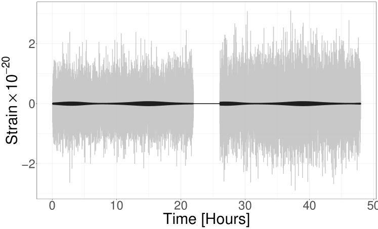
Figure 15: Non-chirping galactic white-dwarf binary GW signal (black) and signal plus noise (grey). A four hour gap is inserted in the middle, multiplied by Tukey-type window (with $r=0.01$). The first half of the noise series is generated using the LISA sensitivity curve in the A TDI channel and the second half is generated using an optical metrology noise modified version of this.

We conduct parameter estimation with the assumption of piecewise stationary noise. This allows us to model the noise PSD before and after the gap differently if they are in fact different (which they are in this example). Even if the noise was stationary, there would be no harm conducting analysis this way. A model that allows for a time-varying noise PSD mitigates against possible parameter estimation biases caused by assuming noise is stationary. We model the two noise PSDs using two independent nonparametric B-spline priors presented in Section III.2.

III.4 Results and Model Checking

We run the MCMC algorithm for 100,000 iterations, with a burn-in of 50,000 and thinning factor of 5. We also use an adaptive proposal for each signal parameter described by Roberts and Rosenthal (2009). That is, for each parameter, we use a standard Metropolis step with Normal proposal centred on the previous value, and variance that is automatically tuned to achieve a desired acceptance rate of 0.44.

As illustrated in Figure 16, we can accurately recover the GW signal parameters in the presence of nonstationary noise due to a simulated planned gap that changes the optical contribution to LISA noise.

Figure 16: Posterior densities for the galactic white dwarf binary parameters. The dashed vertical line is the true parameter.

Model checking, i.e. a careful investigation of the correctness of any model assumptions, should be part of all statistical inference procedures. To check whether it was appropriate to assume that the individual time series before and after the gap were in fact stationary, we can apply the stationarity tests based on the surrogate data approach to the time series of residuals before and after the gap. Moreover, to check whether we could have safely assumed that the full time series is stationary and thus potentially enabled an analysis with one single B-spline prior for the noise component instead of two different noise models, we apply the stationarity test to the residuals of the full time series. The residual time series can be thought of as the “best guess” of underlying noise. We calculate the posterior median GW signal and subtract this from the data to compute the residual series, and then concatenate the residuals before and after the gap. The AR spectrogram of these residuals is highlighted in Figure 17. Running the surrogate tests on the residuals, we report $p$-values (assuming a window length of $T=2^{9}$ and overlap of 75%) in Table 2. For all variants of the surrogate test, we may reject the notion of stationarity for the full residual time series. We also do not reject the hypothesis of stationarity for the first and second halves. This confirms that our stationarity assumptions for each time series before and after the gap was justified and that it was appropriate to assume two different nonparametric noise models.

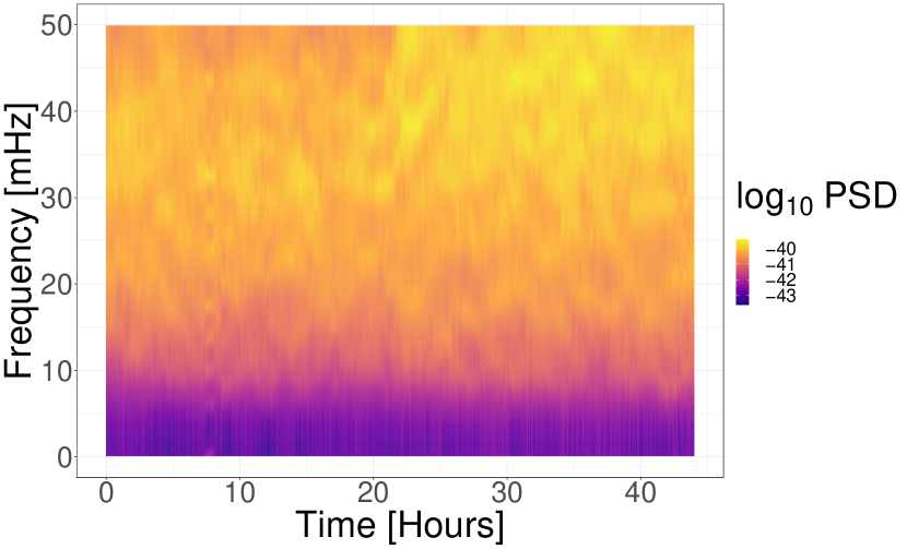
Figure 17: AR spectrogram of residuals after removing the posterior median signal from the data. There is a noticeable change in power at the high frequencies in the second half of the spectrogram.

Table 2: $p$-values of the surrogate tests for the residual time series using a window length of $T=2^{9}$ and overlap 75%.

	KS	KL	LSD	SOMED
Full Series	0.000	0.000	0.001	0.000
Before Gap	0.189	0.492	0.597	0.580
After Gap	0.488	0.445	0.934	0.367

IV Discussion

In this paper, we have discussed methods to identify and address nonstationary noise in the future LISA mission. We demonstrated the usefulness of the lesser-known nonparametric surrogate tests for assessing the stationarity of a time series, introducing a novel variant in the form of the SOMED test. We applied the surrogate tests to real LPF data and showed that certain segments are nonstationary in nature, due to glitches, and amplitude modulations. As the architecture of LISA will share many similarities to LPF, we see this as an important first step in understanding the stationarity/nonstationarity of LISA data.

We introduced a Bayesian semiparametric framework for conducting parameter estimation when there is nonstationary noise as a result of antenna repointing. Assuming a stationary noise model in this situation may lead to systematic biases in astrophysical parameter estimates, as well as larger posterior variances as has been investigated by Chatziioannou et al (2019); Talbot and Thrane (2020); Biscoveanu et al (2020b).

An interesting alternative framework for modelling piecewise stationary noise could be to modify the time-varying spectrum estimation regime of Rosen et al (2012), which utilizes reversible jump MCMC (Green, 1995) to determine the number of locally stationary segments in a time series. One could use a blocked Metropolis-within-Gibbs sampler similar to the one introduced in this paper to model signal parameters given noise parameters and vice versa. This is one avenue we aim to explore in a future paper.

Another future initiative includes investigating the impact of planned data gaps and nonstationary noise on EMRI GW signals, particularly those arising from near-extremal black holes.

References

- Aasi et al (2013) Aasi J, et al (2013) Parameter estimation for compact binary coalescence signals with the first generation gravitational-wave detector network. Physical Review D 88:062,003
- Abbott et al (2020) Abbott BP, et al (2020) A guide to LIGO-Virgo detector noise and extraction of transient gravitational-wave signals. Class Quant Grav 37(5):055,002, DOI 10.1088/1361-6382/ab685e, eprint 1908.11170
- Adams and Cornish (2010) Adams MR, Cornish NJ (2010) Discriminating between a Stochastic Gravitational Wave Background and Instrument Noise. Phys Rev D82:022,002, DOI 10.1103/PhysRevD.82.022002, eprint 1002.1291
- Adams and Cornish (2014) Adams MR, Cornish NJ (2014) Detecting a Stochastic Gravitational Wave Background in the presence of a Galactic Foreground and Instrument Noise. Phys Rev D89(2):022,001, DOI 10.1103/PhysRevD.89.022001, eprint 1307.4116
- Amaro-Seoane et al (2017) Amaro-Seoane P, et al (2017) Laser Interferometer Space Antenna. eprint 1702.00786
- Anderson and Darling (1954) Anderson TW, Darling DA (1954) A test of goodness of fit. Journal of the American Statistical Association 49:765–769
- Armano et al (2016) Armano M, et al (2016) Sub-Femto- free fall for space-based gravitational wave observatories: LISA Pathfinder results. Physical Review Letters 116:231,101, DOI 10.1103/PhysRevLett.116.231101, URL https://link.aps.org/doi/10.1103/PhysRevLett.116.231101
- Armano et al (2018) Armano M, et al (2018) Beyond the required lisa free-fall performance: New LISA pathfinder results down to . Phys Rev Lett 120:061,101, DOI 10.1103/PhysRevLett.120.061101, URL https://link.aps.org/doi/10.1103/PhysRevLett.120.061101
- Armano et al (2019a) Armano M, et al (2019a) Delta release notes. URL http://lpf.esac.esa.int/lpfsa/aio/data-action?ProductType=DOCUMENT&DOCUMENT.DOCUMENT_OID=11850
- Armano et al (2019b) Armano M, et al (2019b) LISA Pathfinder. eprint 1903.08924
- Armano et al (2019c) Armano M, et al (2019c) LISA Pathfinder micronewton cold gas thrusters: In-flight characterization. Phys Rev D 99:122,003, DOI 10.1103/PhysRevD.99.122003, URL https://link.aps.org/doi/10.1103/PhysRevD.99.122003
- Babak and Petiteau (2019) Babak S, Petiteau A (2019) LISA Data Challenge Manual LISA-LCST-SGD-MAN-001
- Baghi et al (2019) Baghi Q, Thorpe JI, Slutsky J, Baker J, Dal Canton T, Korsokova N, Karnesis N (2019) Gravitational-wave parameter estimation with gaps in LISA: a Bayesian data augmentation method. Pre-print arXiv:1907.04747 [gr-qc]
- Baker et al (2019) Baker J, et al (2019) Space Based Gravitational Wave Astronomy Beyond LISA eprint 1907.11305
- Bayram and Baraniuk (2000) Bayram M, Baraniuk R (2000) Multiple window time-varying spectrum estimation. In: Fitzgerald WJ, et al (eds) Nonstationary Signal Processing, Cambridge University Press, Cambridge, pp 292–316
- Biscoveanu et al (2020a) Biscoveanu S, Haster CJ, Vitale S, Davies J (2020a) Quantifying the effect of power spectral density uncertainty on gravitational-wave parameter estimation for compact binary sources. arXiv:200405149
- Biscoveanu et al (2020b) Biscoveanu S, Vitale S, Davies J (2020b) Quantifying the effect of power spectral density uncertainty on gravitational-wave parameter estimation for compact binary sources. arXivorg 102(2), URL http://search.proquest.com/docview/2389079631/
- Borgnat and Flandrin (2009) Borgnat P, Flandrin P (2009) Stationarization via surrogates. Journal of Statistical Mechanics: Theory and Experiment p P01001
- Brockwell and Davis (1991) Brockwell PJ, Davis RA (1991) Time Series: Theory and Methods, 2nd edn. Springer, New York
- Carré and Porter (2010) Carré J, Porter EK (2010) The effect of data gaps on LISA galactic binary parameter estimation. Pre-print arXiv:1010.1641 [gr-qc]
- Chatziioannou et al (2019) Chatziioannou K, Littenberg T, Farr W, Ghonge S, Millhouse M, Clark J, Cornish N (2019) Noise spectral estimation methods and their impact on gravitational wave measurement of compact binary mergers. arXivorg 100(10), URL http://search.proquest.com/docview/2258495700/
- Choudhuri et al (2004) Choudhuri N, Ghosal S, Roy A (2004) Bayesian estimation of the spectral density of a time series. Journal of the American Statistical Association 99(468):1050–1059
- Chua et al (2017) Chua AJK, Moore CJ, Gair JR (2017) The Fast and the Fiducial: Augmented kludge waveforms for detecting extreme-mass-ratio inspirals. Physical Review D 96:044,005
- Dette and Paparoditis (2007) Dette H, Paparoditis E (2007) Testing equality of spectral densities. Technical Report 2007, 29
- Edwards et al (2015) Edwards MC, Meyer R, Christensen N (2015) Bayesian semiparametric power spectral density estimation with applications in gravitational wave data analysis. Physical Review D 92:064,011
- Edwards et al (2019) Edwards MC, Meyer R, Christensen N (2019) Bayesian nonparametric spectral density estimation using B-spline priors. Statistics and Computing 29:67–78
- Efron (1979) Efron B (1979) Bootstrap methods: Another look at the Jackknife. The Annals of Statistics 7:1–26
- Green (1995) Green PJ (1995) Reversible jump Markov chain Monte Carlo computation and Bayesian model determination. Biometrika 82:711–732
- Karnesis et al (2020) Karnesis N, Lilley M, Petiteau A (2020) Assessing the detectability of a stochastic gravitational wave background with LISA, using an excess of power approach. Classical and Quantum Gravity URL http://iopscience.iop.org/10.1088/1361-6382/abb637
- Kirch et al (2018) Kirch C, Edwards MC, Meier A, Meyer R (2018) Beyond Whittle: Nonparametric correction of a parametric likelihood with a focus on Bayesian time series analysis. Bayesian Analysis Advanced publication:1–37
- Kwiatkowski et al (1992) Kwiatkowski D, Phillips PCB, Schmidt P, Shin Y (1992) Testing the null hypothesis of stationarity against the alternative of a unit root. Journal of Econometrics 54:159–178
- Lamberts et al (2019) Lamberts A, Blunt S, Littenberg TB, Garrison-Kimmel S, Kupfer T, Sanderson RE (2019) Predicting the LISA white dwarf binary population in the Milky Way with cosmological simulations. Mon Not Roy Astron Soc 490(4):5888–5903, DOI 10.1093/mnras/stz2834, eprint 1907.00014
- Maturana-Russel and Meyer (2019) Maturana-Russel P, Meyer R (2019) Bayesian spectral density estimation using P-splines with quantile-based knot placement. arXiv:190501832 [statME]
- McCullough and Kareem (2013) McCullough M, Kareem A (2013) Testing stationarity with wavelet-based surrogates. Journal of Engineering Mechanics 139(2):200
- Müller (2005) Müller UK (2005) Size and power of tests of stationarity in highly autocorrelated time series. Journal of Econometrics 128:195–213
- Nason et al (2000) Nason GP, von Sachs R, Kroisandt G (2000) Wavelet processes and adaptive estimation of the evolutionary wavelet spectrum. Journal of Royal Statistical Society B 6:271–292
- Phillips and Perron (1988) Phillips PCB, Perron P (1988) Testing for a unit root in time series regression. Biometrika 75:335–346
- Pollack et al (2010) Pollack SE, Turner MD, Schlamminger S, Hagedorn CA, Gundlach JH (2010) Charge Management for Gravitational Wave Observatories using UV LEDs. Phys Rev D81:021,101, DOI 10.1103/PhysRevD.81.021101, eprint 0912.1769
- Priestley and Subba Rao (1969) Priestley MB, Subba Rao T (1969) A test for non-stationarity of time-series. Journal of the Royal Statistical Society Series B (Methodological) 31:140–149
- Purdue and Larson (2007) Purdue P, Larson SL (2007) Spurious acceleration noise in spaceborne gravitational wave interferometers. Classical and Quantum Gravity 24(23):5869–5887, DOI 10.1088/0264-9381/24/23/010, URL https://doi.org/10.1088%2F0264-9381%2F24%2F23%2F010
- Roberts and Rosenthal (2009) Roberts GO, Rosenthal JS (2009) Examples of adaptive MCMC. Journal of Computational and Graphical Statistics 18:349–367
- Robson and Cornish (2019) Robson T, Cornish NJ (2019) Detecting Gravitational Wave Bursts with LISA in the presence of Instrumental Glitches. Phys Rev D99(2):024,019, DOI 10.1103/PhysRevD.99.024019, eprint 1811.04490
- Robson et al (2019) Robson T, Cornish NJ, Liu C (2019) The construction and use of LISA sensitivity curves. Classical and Quantum Gravity 36(10):105,011, DOI 10.1088/1361-6382/ab1101, URL https://doi.org/10.1088%2F1361-6382%2Fab1101
- Romano and Cornish (2017) Romano JD, Cornish NJ (2017) Detection methods for stochastic gravitational-wave backgrounds: a unified treatment. Living Reviews in Relativity 20:2, DOI https://doi.org/10.1007/s41114-017-0004-1
- Rosen et al (2012) Rosen O, Wood S, Roy A (2012) AdaptSpec: Adaptive spectral density estimation for nonstationary time series. Journal of the American Statistical Association 107:1575–1589
- Rubbo et al (2004) Rubbo LJ, Cornish NJ, Poujade O (2004) Forward modeling of space-borne gravitational wave detectors. Physical Review D 69:082,003
- von Sachs and Neumann (1998) von Sachs R, Neumann MH (1998) A wavelet-based test for stationarity. Journal of Time Series Analysis 21 (5):597–613
- Said and Dickey (1984) Said SE, Dickey DA (1984) Testing for unit roots in autoregressive-moving average models of unknown order. Biometrika 71:599–607
- Sesana et al (2005) Sesana A, Haardt F, Madau P, Volonteri M (2005) The gravitational wave signal from massive black hole binaries and its contribution to the LISA data stream. The Astrophysical Journal 623:23–30
- Swanepoel and Van Wyk (1986) Swanepoel JWH, Van Wyk JWJ (1986) The comparison of two spectral density functions using the bootstrap. Journal of Statistical Computation and Simulation 24:271–282
- Talbot and Thrane (2020) Talbot C, Thrane E (2020) Gravitational-wave astronomy with an uncertain noise power spectral density. arXivorg URL http://search.proquest.com/docview/2411945589/
- Theiler et al (1992) Theiler J, Eubank S, Longtin A, Galdrikian B, Farmer JD (1992) Testing for nonlinearity in time series: the method of surrogate data. Physica D 58:77–94
- Thomson (1982) Thomson DJ (1982) Spectrum estimation and harmonic analysis. Proceedings of the IEEE 70 (9):1055–1096
- Tinto and Dhurandhar (2005) Tinto M, Dhurandhar SV (2005) Time-delay interferometry. Living Reviews in Relativity 8(4)
- Whittle (1957) Whittle P (1957) Curve and periodogram smoothing. Journal of the Royal Statistical Society: Series B (Statistical Methodology) 19:38–63
- Xiao et al (2007) Xiao J, Borgnat P, Flandrin P (2007) Testing stationarity with time-frequency surrogates. Conference Proceedings EUSIPCO-2007, Poznan, Poland pp 2020–2024