Clothoid Fitting and Geometric Hermite Subdivision

Abstract

We consider geometric Hermite subdivision for planar curves, i.e., iteratively refining an input polygon with additional tangent or normal vector information sitting in the vertices. The building block for the (nonlinear) subdivision schemes we propose is based on clothoidal averaging, i.e., averaging w.r.t. locally interpolating clothoids, which are curves of linear curvature. To define clothoidal averaging, we derive a new strategy to approximate Hermite interpolating clothoids. We employ the proposed approach to define the geometric Hermite analogues of the well-known Lane-Riesenfeld and four-point schemes. We present results produced by the proposed schemes and discuss their features. In particular, we demonstrate that the proposed schemes yield visually convincing curves.

1 Introduction

Linear subdivision schemes are widely used in various areas such as geometric modeling, multiscale analysis and for solving PDEs, and are rather well studied; references are for instance [CDM91, DL02, Han18, PR08].

In the last two decades also the interest in nonlinear subdivision schemes has significantly increased. One class of such schemes deals with scalar real valued data, but employs nonlinear averaging/prediction/interpolation techniques, e.g., [DY00, KVD02, CDM03, GVS09], making the corresponding schemes nonlinear. Motivation may be to get more robust estimators for processing data or to be able to deal with discontinuities or nonuniform data. Another class of nonlinear schemes addresses data which live in a nonlinear space, such as a Riemannian manifold or a Lie group, see for instance [WD05, XY09, Gro10, Wei10, Moo16]. A third class considers data living in Euclidean space, typically of dimension $2$ or $3$, but the averaging rules are nonlinear to take account of their geometric characteristics. Such rules may be formulated in terms of angles, perpendicular bisectors, interpolating circles, and the like, rather than acting on each component separately, as linear schemes do. References of such geometric schemes include [AEV03, SD04, MDL05, DFH09, CHR13].

In contrast to linear schemes, for which a rather well established analysis is available, nonlinear schemes are less well understood, and there are ongoing efforts to devise new and to improve existing tools. However, due to the nonlinear nature and the diversity of the proposed schemes, not as general results as in the linear case can be expected. The investigation of a particular class of nonlinear schemes is likely to require an additional particular analysis component not covered by a general theory. Papers providing an analysis framework for geometric curve subdivision are [DH12, ERS15]. The first reference derives sufficient conditions for a convergent interpolatory planar subdivision scheme to produce tangent continuous limit curves. The second reference deals with subdivision schemes which are geometric in the sense that they commute with similarities and derives a framework to establish $C^{1,\alpha}$- and $C^{2,\alpha}$-regularity of the generated limit curves.

In this paper, we present a family of geometric Hermite subdivision schemes for the generation of planar curves where the data to be refined are point-vector pairs, the latter serving as information on tangents or normals. Schemes refining point-vector pairs of that type were already suggested in [CJ07, LD16]. The basic idea of these two approaches is to locally fit circles to the data and then to sample new points from them, but the specific methods are different. Also the strategies for determining new vectors are not the same so that the two schemes have significantly different shape properties. In contrast, the approach proposed here relies on clothoids, which are curves of linear curvature, rather than circles. The top row of Figure 1 shows the refinement of initial data consisting of two point-normal pairs by the so-called clothoid average, as described in this paper. The resulting curve is S-shaped and interpolates the initial data. Also the scheme of Chalmoviansky and Jüttler [CJ07], as shown in the middle row, interpolates the initial data, but has three turning points, leading to a less natural shape and a less optimal distribution of curvature. The scheme of Dyn and Lipovetsky [LD16], shown in the bottom row, produces a straight line (as it would for any choice of parallel normals). This is likely not to address the designer’s intent, and it also does not interpolate the normal directions specified at the endpoints. The good performance of our scheme is related to the fact that it is not based on the reproduction of circles, which can be seen as the geometric analogue of quadratic polynomials, but on the reproduction of clothoids, which can be seen as the geometric analogue of cubic polynomials. Thus, it is able to mimic a much larger variety of shapes.

The idea of geometric planar spline fitting, i.e., fitting splines based on clothoids as building blocks can be traced through the literature for more than 50 years [BdB65, Sto82, Meh74, MW92, HL92, Coo93]. Further recent contributions are for instance [BF18] presenting an alternative to [Sto82] for the computation of a $C^{2}$ interpolating clothoid spline. Hermite interpolation problems w.r.t. clothoids are for instance the topic of [BF15]. We also point out [MW09] where the authors employ so called e-curves as approximative substitutes for clothoids in the context of Hermite interpolation.

Maybe the two striking reason why clothoid splines and approximations of them are still a topic in the literature are as follows: (i) the corresponding clothoid splines are rather expensive two compute; (ii) there are plenty of applications. Let us discuss these points in more details. Concerning (ii), for a long time clothoids have been used by route designers as transitional curves between straight lines and circular arcs, and between circular arcs of different radii; see for instance [MW90, Baa84]. Nowadays, they are further used in connection with path planning for autonomous vehicles, e.g., [Ber15, AGRA15, BLR⁺12] in computer vision and image processing [KFP03, BL15], in curve editing for design purposes [HEWF13] or representing hand-drawn strokes sketched by a user [MS09, BLP10]. Concerning (i), many of the above applications are rather time critical and it is often important to have algorithms which are as fast as possible at a given (sometimes moderate) approximation quality. Solving clothoidal spline fitting problems up to high precision can be done rather fast [Sto82] but even this is sometimes too expensive or not needed. Instead, frequently faster strategies typically using some approximation are employed. For instance, [BLP10] locally fits clothoids and arcs as primitives and then optimizes w.r.t. a certain graph to obtain a global fit. The paper [HEWF13] uses a variational approach iteratively inserting control points and optimizing them such as to generate a polyline with linear discrete curvature (approximating the clothoid segment; for details see also [SK00].) We mention that this approach uses subdivision (explicitly the analogue of corner cutting) for clothoid blending. Other approaches replace clothoids by approximating curve segments which are easier to handle, e.g., [MW04, MW09]. We point out that the clothoidal subdivision schemes suggested here may be used as a computationally rather cheap alternative to clothoid splines and that they may be employed in the various applications discussed above.

The paper is organized as follows: After presenting some basic facts about two-point Hermite interpolation with clothoids in the next section, we consider its approximate solution in Section 3. The formula we propose is explicit, fast to evaluate, and yields a very small error for a large range of input data. In Section 4, this result is used to define the so-called clothoid average of a pair of points and corresponding tangent directions, which in turn serves as a building block for new families of geometric Hermite subdivision schemes. In particular, we obtain geometric Hermite analogues of the Lane-Riesenfeld schemes and the four-point scheme. In Section 5, we present results produced by the proposed schemes and discuss their features to illustrate the potential of the new method. As a first theoretical result, Section 6 establishes convergence and $G^{1}$-continuity of the Lane-Riesenfeld-type algorithm of degree $1$. Concluding remarks and an outlook are given in Section 7.

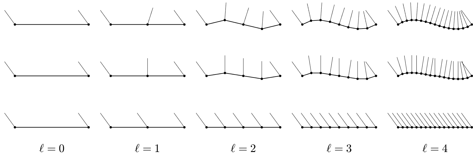
Figure 1: Midpoint refinement using the proposed clothoid average (upper row), the circle average of [CJ07] (middle row), and the circle average of [LD16] (lower row). We always display the points $p_{j}^{\ell}$ together with the normals $n^{\ell}_{j}=i\exp(i\alpha^{\ell}_{j})$ at level $\ell$.

2 Two-point interpolation

In the following, points in the plane, and in particular images of planar curves, are considered as complex numbers. In this sense, let $p:[0,1]\to\mathbb{C}$ be a twice differentiable function parametrizing a planar curve which is regular in the sense that the velocity $v:=|p^{\prime}|$ vanishes nowhere. It is called uniform if the velocity is constant. According to the lifting lemma, the tangent vector can be expressed in the form $p^{\prime}=v\exp(i\alpha)$ with a differentiable function $\alpha:[0,1]\to\mathbb{R}$, called the tangent angle of $p$. We write $\alpha=\arg p^{\prime}$ for brevity, and assume throughout that $\alpha$ is unrolled suitably so that jumps are avoided. The curvature of $p$ is $\kappa:=\alpha^{\prime}/v=\operatorname{Im}\bar{p}^{\prime}p^{\prime\prime}/v^{3}$. In the uniform case, on which we focus below, curve, velocity, and tangent angle are related by the formula

$$p(t)=p(0)+v\int_{0}^{t}\exp(i\alpha(s))\,ds,\quad t\in[0,1].$$ (1a)

The integral appearing here is abbreviated by

$$I(\alpha,t):=\int_{0}^{t}\exp(i\alpha(s))\,ds,\quad I(\alpha):=I(\alpha,1),$$

so that $p=p(0)+vI(\alpha,\cdot)$. A curve $q:[0,1]\to\mathbb{C}$ starting at $q_{0}:=q(0)=0$ and ending at $q_{1}:=q(1)\in\mathbb{R}^{+}$ is said to be in normal position. To tell this from the general case, we use the letters $w=|q^{\prime}|,\beta=\arg q^{\prime}$, and $\lambda=\beta^{\prime}/w$ to denote the velocity, tangent angle, and curvature, respectively. We have the relation

$$q(t)=wI(\beta,t),\quad t\in[0,1].$$ (1b)

Curves in general and normal position are linked by similarity. Denoting the secant between the endpoints of $p$ by $d:=p_{1}-p_{0}$ and its angle by $\varphi:=\arg d$, we have the relations

$$p=p_{0}+\frac{d}{q_{1}}q,\quad v=\frac{|d|}{q_{1}}w,\quad\alpha=\beta+\varphi.$$ (2)

Let $J=\{0,1\}$. Given points $p_{J}=(p_{0},p_{1})$ with $d:=p_{1}-p_{0}\neq 0$ and angles $\alpha_{J}=(\alpha_{0},\alpha_{1})$, the corresponding two-point Hermite interpolation problem is to find a curve $p$ such that

$$p(j)=p_{j},\quad\alpha(j)=\alpha_{j},\quad j\in J.$$ (3)

A special case of the above problem is to find a curve $q$ such that

$$q(j)=j,\quad\beta(j)=\beta_{j},\quad j\in J,$$ (4)

for given $\beta_{J}$. We recall that we use letters $q,\beta$ to indicate that the sought curve is in normal position. Figure 2 illustrates the setting. While it is simple to specify curves merely satisfying these constraints, the challenge is to find solutions which are fair in some sense. For instance, it is a classical task to solve (3) in the space of clothoids, which are curves characterized by a linear curvature profile. In principle, this nonlinear problem is well understood and various more or less complicated methods for its numerical treatment are described in the literature, see for instance [WM09, BF15] and the references therein. Before we present our own approximate approach in the next section, we introduce some notation and basic facts.

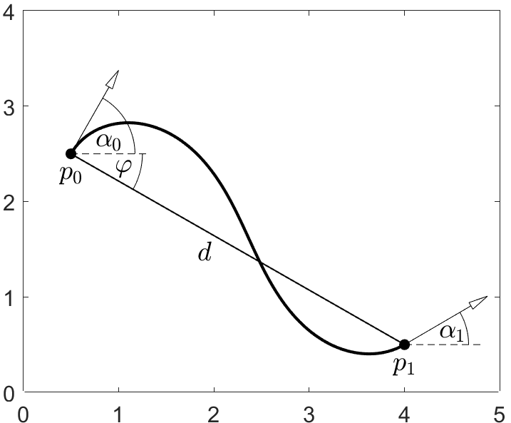
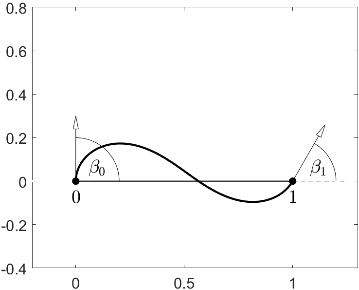
Figure 2: Interpolation problem in general position (left) and normal position (right).

Using the symbol $\mathbb{P}_{n}$ to denote the space of polynomials of degree at most $n$ over the unit interval, we define

$${\mathcal{K}}_{n}:=\{p:\kappa\in\mathbb{P}_{n}\}$$

as the set of all uniform curves $p:[0,1]\to\mathbb{C}$ with curvature in $\mathbb{P}_{n}$. The corresponding subset of such curves in normal position is denoted by ${\mathcal{K}}_{n}^{+}$. In particular, ${\mathcal{K}}_{0}$ contains straight lines and circular arcs, while curves in ${\mathcal{K}}_{1}\setminus{\mathcal{K}}_{0}$ are segments of clothoids. The tangent angle $\alpha=\int\kappa$ of a clothoid is a quadratic polynomial. For clothoids, the integral appearing in (1a) can be transformed to the so-called Fresnel integral $F(x):=\int_{0}^{x}\exp(iu^{2})\,du$, which does not possess a finite representation with respect to elementary functions. For later use we state the following lemma.

Lemma 2.1

A regular curve $p\in{\mathcal{K}}_{1}$ is embedded unless it parametrizes a full circle, i.e., unless $p\in{\mathcal{K}}_{0}$ and $|\alpha_{1}-\alpha_{0}|\geq 2\pi$.

The proof follows immediately form the Tait-Kneser Theorem.

In the following, for simplicity of wording, the term clothoid addresses not only segments of true clothoids, but also segments of circles and straight lines. In this sense, we consider the solution of (3) with clothoids, i.e., with curves $p\in{\mathcal{K}}_{1}$. By similarity according to (2), this problem can be reduced to (4) with data $\beta_{J}=\alpha_{J}-\arg d$, which are the angles between the secant $d$ and the boundary tangent angles of $p$. Using the quadratic Lagrange polynomials

$$\ell^{2}_{0}:=(t-1)(2t-1),\quad\ell^{2}_{1/2}(t):=4t(1-t),\quad\ell^{2}_{1}(t):=t(2t-1),$$

with respect to the break points $0,1/2,1$, the tangent angle of $q$ can be written as

$$\beta=\beta_{0}\ell^{2}_{0}+\beta_{1/2}\ell^{2}_{1/2}+\beta_{1}\ell^{2}_{1}.$$

Hence, given $\beta_{J}$, the sought solution is characterized by the value $\beta_{1/2}=\beta(1/2)$ and the velocity $w$ by means of (1b). The task is to find these two values. Figure 3 demonstrates that the solution of (4) is not unique. More precisely, it is known that for each pair $\beta_{J}$ there exists a countable family of solutions, but in applications, one is typically interested in curves avoiding excess rotation. For instance, if the boundary data $\beta_{J}$ are small in modulus, also the overall maximum $\|\beta\|_{\infty}$ of tangent angles should be small. The following theorem guarantees existence of such a solution.

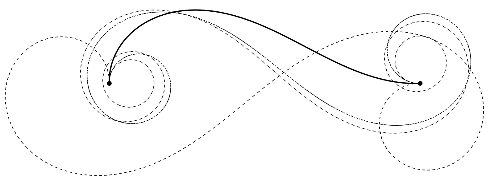
Figure 3: Four out of infinitely many clothoid solutions to the geometric Hermite interpolation problem (4) with angles $\beta_{0}=\pi/2,\beta_{1}=0$. The solid line shows the preferred choice, which avoids excess rotation.

Theorem 2.2

There exists a smooth function $F:U\to\mathbb{R}^{2}$, defined on some neighborhood $U=(-u,u)^{2}$ of the origin, with

$$F(0,0)=\begin{bmatrix}0\\ 1\end{bmatrix},\quad DF(0,0)=\begin{bmatrix}-1/4&-1/4\\ 0&0\end{bmatrix},$$

and the following property: Let

$$\begin{bmatrix}\beta_{1/2}\\ w\end{bmatrix}:=F(\beta_{0},\beta_{1}),\quad\beta:=\beta_{0}\ell^{2}_{0}+\beta_{1/2}\ell^{2}_{1/2}+\beta_{1}\ell^{2}_{1},$$

then the tangent angle $\beta$ and the velocity $w$ define a solution $q=wI(\beta,\cdot)\in{\mathcal{K}}_{1}^{+}$ of (4). In particular, $I(\beta)=1/w$ is real and positive.

Actually, it is possible to choose the domain $U=(-\pi,\pi)^{2}$ for $F$, covering almost all possible pairs of boundary tangent angles, but this is not needed here.

Proof. The idea is to parametrize the set solutions of (4) for varying $\beta_{J}$ as a two-dimensional surface in $\mathbb{R}^{4}$ and then to apply the implicit function theorem. Given $\alpha_{J}\in\mathbb{R}^{2}$, define the tangent angle $\alpha:=\alpha_{0}\ell^{2}_{0}+\alpha_{1}\ell^{2}_{1}$ and the clothoid $p:=I(\alpha,\cdot)\in{\mathcal{K}}_{1}$. Then $q:=p/p(1)\in{\mathcal{K}}_{1}^{+}$ connects $q(0)=0$ and $q(1)=1$. Its velocity is $w=1/|p(1)|$, and its tangent angle $\beta=\alpha-\arg p(1)$ has values $\beta_{j}:=\beta(j)=\alpha_{j}-\arg p(1),j\in J,$ and $\beta_{1/2}:=\beta(1/2)=-\arg p(1)$. With these data, we define the surface $\Phi(\alpha_{0},\alpha_{1}):=[\beta_{1/2},w,\beta_{0},\beta_{1}]^{T}$. It is well defined and smooth in a neighborhood of the origin since $p(1)=1$ for $\alpha_{0}=\alpha_{1}=0$. Let $\|\alpha_{J}\|_{\infty}=h$. Then $\|\alpha\|_{\infty}=h$ and

$$p(1)=1+\int_{0}^{1}i\alpha(s)\,ds+O(h^{2})=1+i\,\frac{\alpha_{0}+\alpha_{1}}{6}+O(h^{2})$$

so that $w=1+O(h^{2})$ and $\arg p(1)=(\alpha_{0}+\alpha_{1})/6+O(h^{2})$. We conclude that

$$\Phi(0,0)=\begin{bmatrix}0\\ 1\\ 0\\ 0\end{bmatrix},\quad D\Phi(0,0)=\frac{1}{6}\begin{bmatrix}-1&-1\\ 0&0\\ 5&-1\\ -1&5\end{bmatrix},$$

are value and derivative of $\Phi$ at the origin. The lower $(2\times 2)$-submatrix of $D\Phi(0,0)$ has determinant $2/3$. Hence, by the implicit function theorem, there exists a neighborhood $U$ of the origin and a smooth function $F:U\to\mathbb{R}^{2}$ such that $[F(\beta_{J}),\beta_{J}]^{T}$ defines a point on the trace of $\Phi$ for all $\beta_{J}\in U$, corresponding to the clothoid solving (4). Value and derivative of $F$ at the origin are given by

$$F(0,0)=\begin{bmatrix}0\\ 1\end{bmatrix},\quad DF(0,0)=\begin{bmatrix}-1&-1\\ 0&0\end{bmatrix}\cdot\begin{bmatrix}5&-1\\ -1&5\end{bmatrix}^{-1}=\begin{bmatrix}-1/4&-1/4\\ 0&0\end{bmatrix}.$$

One might suspect that employing functions $\alpha$ of the general form $\alpha=\alpha_{0}\ell^{2}_{0}+\alpha_{1/2}\ell^{2}_{1/2}+\alpha_{1}\ell^{2}_{1}$ would define even more solutions of (4). To see that this is not true, let $\tilde{\alpha}:=\alpha-\alpha_{1/2}=(\alpha_{0}-\alpha_{1/2})\ell^{2}_{0}+(\alpha_{1}-\alpha_{1/2})\ell^{2}_{1}$ be an angle function as considered above. Then the corresponding clothoids $p:=I(\alpha,\cdot)$ and $\tilde{p}:=I(\tilde{\alpha},\cdot)$ are related by $p=\exp(i\alpha_{1/2})\tilde{p}$ so that their normal forms coincide,

$$q=\frac{p}{p(1)}=\frac{\exp(i\alpha_{1/2})\tilde{p}}{\exp(i\alpha_{1/2})\tilde{p}(1)}=\frac{\tilde{p}}{\tilde{p}(1)}=\tilde{q}.$$

$\square$

Let $p_{J},\alpha_{J}$ be boundary data for the general problem (3) with $d=p_{1}-p_{0}\neq 0$. If $q$ is the solution of (4) for data $\beta_{J}:=\alpha_{J}-\arg d$ according to the preceding theorem, then $p:=p_{0}+dq$ solves (3). With $q=wI(\beta,\cdot)$, an equivalent expression is

$$p=p_{0}+\frac{d}{I(\beta)}I(\beta,\cdot),$$ (5)

which is independent of the velocity $w$. Hence, it suffices to know the first coordinate function

$$f:U\to\mathbb{R},\quad f(\beta_{0},\beta_{1})=\beta_{1/2},$$

of $F$ to construct the crucial tangent angle $\beta:=\beta_{0}\ell^{2}_{0}+f(\beta_{0},\beta_{1})\ell^{2}_{1/2}+\beta_{1}\ell^{2}_{1}$.

The function $f$ has the symmetry properties

$$f(\beta_{0},\beta_{1})=f(\beta_{1},\beta_{0}),\quad f(-\beta_{0},-\beta_{1})=-f(\beta_{0},\beta_{1}).$$ (6)

Hence, the second order derivatives vanish at the origin and we obtain the expansion

$$f(\beta_{0},\beta_{1})=-\frac{\beta_{0}+\beta_{1}}{4}+O(\|\beta_{J}\|^{3}).$$

3 Approximate solution

Computing accurate solutions of the nonlinear problem (4) is possible, but the determination of $\beta_{1/2}=f(\beta_{0},\beta_{1})$ requests more or less elaborate and/or computationally expensive numerical methods. Instead, we propose a good approximation $\tilde{f}$ for later use with subdivision algorithms. More precisely, we seek a function $\tilde{f}$ with the following properties:

• $\tilde{f}:\mathbb{R}^{2}\to\mathbb{R}$ is a cubic polynomial. This choice combines modest complexity with sufficient flexibility to achieve good global approximation.

• $\tilde{f}(0,0)=f(0,0)$ and $D\tilde{f}(0,0)=Df(0,0)$. Thus, $\tilde{f}$ approximates $f$ very good for small data.

• $\tilde{f}$ inherits the symmetry properties (6) from $f$,

  $$\tilde{f}(\beta_{0},\beta_{1})=\tilde{f}(\beta_{1},\beta_{0}),\quad\tilde{f}(-\beta_{0},-\beta_{1})=-\tilde{f}(\beta_{0},\beta_{1}).$$

• For a wide range of boundary data, say $\beta_{J}\in B:=[-\pi/2,\pi/2]^{2}$, the angle defect

  $$\delta(\beta_{J}):=\arg I(\beta),\quad\beta:=\beta_{0}\ell^{2}_{0}+\tilde{f}(\beta_{0},\beta_{1})\ell^{2}_{1/2}+\beta_{1}\ell^{2}_{1}$$

  is small in modulus.

Before presenting our solution, let us explain the meaning of the angle defect as a measure for the quality of the approximation $\tilde{f}$.

Theorem 3.1

Given Hermite data $p_{J},\alpha_{J}$ with $d=p_{1}-p_{0}\neq 0$, let $\beta_{J}:=\alpha_{J}-\arg d$ and $\beta:=\beta_{0}\ell^{2}_{0}+\tilde{f}(\beta_{0},\beta_{1})\ell^{2}_{1/2}+\beta_{1}\ell^{2}_{1}$, as above. Then, analogous to (5),

$$p:=p_{0}+\frac{d}{I(\beta)}I(\beta,\cdot)$$

defines a clothoid interpolating the point data, i.e., $p(0)=p_{0},p(1)=p_{1}$. At the boundaries, its tangent angle $\alpha$ differs from the prescribed values by the angle defect,

$$\alpha(0)=\alpha_{0}-\delta(\beta_{J}),\quad\alpha(1)=\alpha_{1}-\delta(\beta_{J}).$$

Proof. Interpolation of the point data is trivial. For the tangent angle, we obtain

$$\alpha(j)=\arg d+\beta(j)-\arg I(\beta)=\arg d+\beta_{j}-\delta(\beta_{J})=\alpha_{j}-\delta(\beta_{J}),\quad j\in J.$$

$\square$

To construct a suitable function $\tilde{f}$, we adopt the idea used in the proof of Theorem 2.2. For a large collection of angles $\alpha_{J}^{i},i\in I$, we compute points $\Phi(\alpha^{i}_{0},\alpha^{i}_{1})=[\beta^{i}_{1/2},w^{i},\beta^{i}_{0},\beta^{i}_{1}]^{T}$ representing clothoids in normal position. Points for which one of the angles $\beta^{i}_{0},\beta^{i}_{1/2},\beta^{i}_{1}$ lies outside the interval $B$ are discarded as they correspond to clothoids with too large tangent angles, which are of little relevance for most applications, e.g., for design purposes. Denoting the index set of the remaining points by $\tilde{I}$, the task is to determine $\tilde{f}$ such that $f(\beta^{i}_{0},\beta^{i}_{1})\approx\beta^{i}_{1/2}$ for all $i\in\tilde{I}$. The ansatz for the cubic polynomial $\tilde{f}$ satisfying ii) with symmetry properties according to iii) is

$$f(\beta_{0},\beta_{1})=(\beta_{0}+\beta_{1})\bigl{(}f_{1}(\beta_{0}^{2}+\beta_{1}^{2})+f_{2}\beta_{0}\beta_{1}-1/4\bigr{)}.$$

Now, we can determine the unknown parameters $f_{0},f_{1}$ by standard approximation methods. The following choice was found when striving for a good compromise between the maximal angle defect $\|\delta(\beta_{J})\|_{\infty}$ and simplicity of the coefficients.

Theorem 3.2

Let

$$\tilde{f}(\beta_{0},\beta_{1}):=(\beta_{0}+\beta_{1})\left(\frac{\beta_{0}^{2}+\beta_{1}^{2}}{68}-\frac{\beta_{0}\beta_{1}}{46}-\frac{1}{4}\right).$$ (7)

There exist constants $c_{1},c_{2}$ such that the angle defect is bounded by

$$|\delta(\beta_{0},\beta_{1})|\leq\min\{c_{1},c_{2}|\beta_{0}+\beta_{1}|\cdot\|\beta_{J}\|^{2}\}$$

for all $\beta_{J}\in B:=[-\pi/2,\pi/2]^{2}$. A feasible numerical value for both constants is $c_{1}=c_{2}=1/800$, which is less than a $1/800$.

Proof. Boundedness of the angle defect by some constant $c_{1}$ follows immediately from continuity over the compact domain $B$. Concerning existence of a bound in terms of $|\beta_{0}+\beta_{1}|\cdot\|\beta_{J}\|^{2}$, we note that properties ii) and iii) together with (6) imply that $f(\beta_{J})-\tilde{f}(\beta_{J})=O(\|\beta\|^{3})$ and $f(\beta_{J})=\tilde{f}(\beta_{J})=0$ for $\beta_{0}+\beta_{1}=0$. Thus, there exists a constant $\tilde{c}_{2}$ such that

$$|f(\beta_{J})-\tilde{f}(\beta_{J})|\leq\tilde{c}_{2}|\beta_{0}+\beta_{1}|(\beta_{0}^{2}+\beta_{1}^{2}),\quad\beta_{J}\in U.$$

It remains to show that this qualitative behavior is inherited by $\delta$. To this end, we define the function

$$\Delta(\beta_{J},\beta_{1/2}):=\bigl{|}\arg I(\beta)\bigr{|},\quad\beta_{J}\in B,\ \beta_{1/2}\in f(B)\cup\tilde{f}(B),$$

with $\beta=\beta_{0}\ell^{2}_{0}+\beta_{1}\ell^{2}_{1}+\beta_{1/2}\ell^{2}_{1/2}$. Since $|\beta_{1}-\beta_{0}|<2\pi$ for $\beta_{J}\in B$, Lemma 2.1 implies that the integral is nonzero so that $\Delta$ is a smooth function over a compact domain and hence Lipschitz with some constant $L$. We obtain

$$\delta(\beta_{J}) =\Delta(\beta_{J},\tilde{f}(\beta_{J}))=\Delta(\beta_{J},\tilde{f}(\beta_{J}))-\Delta(\beta_{J},f(\beta_{J}))$$

$$\leq L|\tilde{f}(\beta_{J})-f(\beta_{J})|\leq\tilde{c}_{2}L|\beta_{0}+\beta_{1}|(\beta_{0}^{2}+\beta_{1}^{2})$$

for $\beta_{J}\in U$. For $\beta_{J}\not\in U$, continuity of $\delta$ shows that the inequality remains valid with a possibly enlarged constant $c_{2}$. The given numerical value for $c_{1}$ and $c_{2}$ can be verified by evaluation over a fine grid on $B$, see Figure 4. $\square$

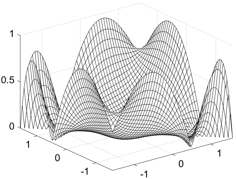
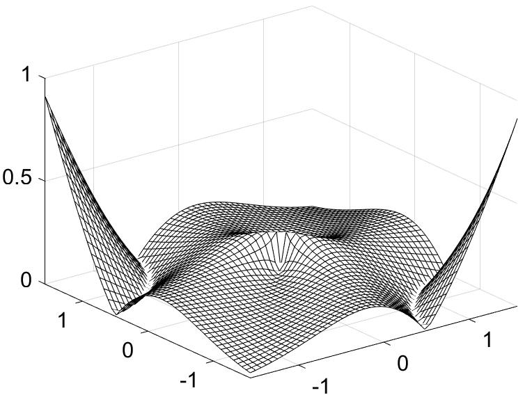
Figure 4: Plots of $800\cdot|\delta(\beta_{J})|$ (left) and $800\cdot|\delta(\beta_{J})|/(|\beta_{0}+\beta_{1}|(\beta_{0}^{2}+\beta_{1}^{2}))$ (right) for $-\pi/2\leq\beta_{0},\beta_{1}\leq\pi/2$. The upper bound $1$ in both cases indicates that $c_{1}=c_{2}=1/800$ is a feasible value for the constants in Theorem 3.2.

In many applications, an error of less than a tenth of a degree for the interpolation of tangent angles will be acceptable so that the given approximation can be used directly. Moreover, the theorem shows that the approximation is exact for the symmetric case $f(\beta_{0},-\beta_{0})=\tilde{f}(\beta_{0},-\beta_{0})=0$, whose solution is a segment of a circle or a straight line.

If, in the general case, higher accuracy is required, one step of the Newton iteration

$$\beta_{1/2}\quad{\mathrel{\reflectbox{$\longmapsto$}}}\quad\beta_{1/2}-\arg I(\beta)/\operatorname{Re}\left(\frac{\int_{0}^{1}\ell^{2}_{1/2}(t)\exp(i\beta(t))\,dt}{I(\beta)}\right)$$

reduces the maximal angle defect to less than $5\!\times\!10^{-8}$, and a second step to less than $5\!\times\!10^{-16}$.

4 Hermite subdivision by the clothoid average

If a whole sequence of Hermite data points is to be interpolated, one might join always two of them by a clothoid and connect the segments to form a single composite curve. If the clothoids are determined exactly, their contact is $G^{1}$, meaning that points and tangent directions of neighboring clothoids coincide at the junctions. If the clothoid is only approximated, as described in the preceding section, the contact is still continuous, but not $G^{1}$ in a strict sense. In any case, curvature is discontinuous, what may be insufficient for many design applications. Below, we propose different subdivision strategies to generate a (visually) smooth curve from a sequence $p_{j}^{0}$ of points in $\mathbb{C}$ and corresponding tangent angles $\alpha_{j}^{0},j\in\mathbb{Z}$. As building block we define the (approximate) clothoid average as follows:

Definition 4.1

Given a pair of Hermite couples $h_{j}:=(p_{j},\alpha_{j}),j\in J$, with $d:=p_{1}-p_{0}\neq 0$, let $p\in{\mathcal{K}}_{1}$ be the clothoid with endpoints $\tilde{p}(j)=p_{j}$ and tangent angles $\alpha(j)\approx\alpha_{j}$ constructed by the approximation $\tilde{F}$ of $F$ according to Theorem 3.2. Then the approximate clothoid average of $h_{0}$ and $h_{1}$ at $t\in\mathbb{R}$ is defined by evaluation of $p$ and the corresponding angle function $\alpha$ at $t$, and written as

$$th_{0}\oplus(1-t)h_{1}:=\bigl{(}p(t),\alpha(t)\bigr{)}.$$

Sequences of Hermite couples are denoted by $H:=(h_{j})_{j\in\mathbb{Z}}$. Now, we generate sequences $H^{0},H^{1},H^{2},\dots$ from given initial data $H^{0}$ by means of a binary subdivision operator $S:H^{\ell}\to H^{\ell+1}$, the rules of which are based on the clothoid average.

The simplest subdivision operator of that type is inserting a new Hermite couple always between two given ones,

$$S_{1}:=H\mapsto H^{\prime},\quad h^{\prime}_{2j}=h_{j},\quad h^{\prime}_{2j+1}=\frac{1}{2}h_{j}\oplus\frac{1}{2}h_{j+1}.$$

Formally, $S_{1}$ corresponds to the Lane-Riesenfeld algorithm of degree $1$. Defining the averaging operator

$$A:=H\mapsto H^{\prime},\quad h^{\prime}_{j}=\frac{1}{2}h_{j}\oplus\frac{1}{2}h_{j+1},$$

we can proceed in that direction and define Lane-Riesenfeld-type algorithms of degree $n$ by applying $(n-1)$ rounds of averaging to the output of $S_{1}$,

$$S_{n}:=A^{n-1}S_{1},\quad n\in\mathbb{N}.$$

For instance, the Chaikin-type algorithm, obtained for $n=2$, explicitly reads

$$S_{2}:=H\mapsto H^{\prime},\quad h^{\prime}_{2j}=\frac{1}{2}h_{j}\oplus\frac{1}{2}\Bigl{(}\frac{1}{2}h_{j}\oplus\frac{1}{2}h_{j+1}\Bigr{)},\quad h^{\prime}_{2j+1}=\frac{1}{2}\Bigl{(}\frac{1}{2}h_{j}\oplus\frac{1}{2}h_{j+1}\Bigr{)}\oplus\frac{1}{2}h_{j+1}.$$

Needless to say that this symbolic representation of a nonlinear process cannot be simplified through commutativity, associativity, or distributivity.

As a further example, we define a family of interpolatory four-point schemes $S^{4}_{\omega}$ with tension parameter $\omega<0$,

$$S^{4}_{\omega}:=H\mapsto H^{\prime},\quad h^{\prime}_{2j}:=h_{j},\quad h^{\prime}_{2j+1}:=\frac{1}{2}\bigl{(}\omega h_{j-1}\oplus(1-\omega)h_{j}\bigr{)}+\frac{1}{2}\bigl{(}(1-\omega)h_{j+1}\oplus\omega h_{j+2}\bigr{)}.$$

Of course, many other subdivision schemes, including schemes of arbitrary arity, can be constructed in this spirit.

Let $H^{\ell}=S^{\ell}H^{0}=(h^{\ell}_{j})_{j\in\mathbb{Z}}$ be the sequence of Hermite couples $h^{\ell}_{j}=(p^{\ell}_{j},\alpha^{\ell}_{j})$ at level $\ell\in\mathbb{N}_{0}$. A common feature of the algorithms presented above is the reproduction of circles. That is, if there exists a midpoint $m\in\mathbb{C}$ and a radius $r>0$ such that $p^{\ell}_{j}=m-ir\exp(i\alpha^{\ell}_{j})$ for all $j$, then $p^{\ell+1}_{j}=m-ir\exp(i\alpha^{\ell+1}_{j})$ for all $j$. Further, clothoids are almost reproduced. That is, if $p\in{\mathcal{K}}_{1}$ is a clothoid with angle function $\alpha$, and if

$$p^{\ell}_{j}=p(t^{\ell}_{j}),\quad\alpha^{\ell}_{j}=\alpha(t^{\ell}_{j}),\quad j\in\mathbb{Z},$$

for certain parameters $t^{\ell}_{j}$, then there exist parameters $t^{\ell+1}_{j}$ such that

$$p^{\ell+1}_{j}\approx p(t^{\ell+1}_{j}),\quad\alpha^{\ell+1}_{j}\approx\alpha(t^{\ell+1}_{j}),\quad j\in\mathbb{Z}.$$

The quality of the approximation is determined by the magnitude of the angle defect according to the preceding section.

Concerning convergence, the examples in the next section suggest that all algorithms presented here are $G^{1}$-convergent in the following sense: There exists a curve $p$ in $\mathbb{C}$ with tangent angle $\alpha$ which, respectively, are the limits of points and angles generated by the algorithm. More precisely, if $j(\ell)$ is a sequence of integers such that $t=\lim_{\ell\to\infty}2^{-\ell}j(\ell)$, then

$$\lim_{\ell\to\infty}p^{\ell}_{j(\ell)}=p(t)\quad\text{and}\quad\lim_{\ell\to\infty}\alpha^{\ell}_{j(\ell)}=\arg p^{\prime}(t)=\alpha(t).$$

This is analogous to standard Hermite subdivision, where the slope of the limit must coincide with the limit of slopes, and that is why we suggest to call the procedures introduced here Geometric Hermite subdivision. A proof of $G^{1}$-convergence of the Lane-Riesenfeld-type algorithm $S_{1}$ of degree $1$ is given in Section 6; a more general theory is currently developed and beyond the scope of this paper.

5 Numerical Experiments

In this section, we present numerical examples illustrating the shape properties of the Hermite subdivision algorithms $S_{n}$ and $S^{4}_{\omega}$ as introduced in the preceding section.

Throughout, we use the same set of initial data $H^{0}$. To avoid a special treatment of boundaries, it is assumed to be periodic, $h^{0}_{j}=h^{0}_{j+8},j\in\mathbb{Z}$. All figures are structured as follows: On the left hand side, we see the initial points $p^{0}_{j}$ and normals $n^{0}_{j}:=i\exp(i\alpha_{j}^{0})$ together with the polygon $p^{\ell}_{j}$ as obtained after $\ell=8$ rounds of subdivision. The middle figure shows the points $p^{\ell}_{j}$ for $\ell=5$ together with the corresponding normals $n^{\ell}_{j}:=i\exp(i\alpha_{j}^{\ell})$. On the right hand side, estimated curvature values $\kappa^{\ell}_{j},\ell=8,$ are plotted versus the normalized chord length

$$s_{j}^{\ell}:=\sigma\sum_{i=0}^{j-1}\bigl{|}p^{\ell}_{i+1}-p^{\ell}_{i}\bigr{|},$$

where $\sigma$ is chosen such that the length of one loop equals $1$. Specifically, the curvature value $\kappa^{\ell}_{j}$ is computed as the reciprocal radius of the circle interpolating the points $p^{\ell}_{j-1},p^{\ell}_{j},p^{\ell}_{j+1}$. The Fresnel-integrals $I(\alpha,\cdot)$ appearing in the definition of the clothoid average are computed using Gauss-Legendre quadrature with three nodes.

Figure 5 shows the Lane-Riesenfeld-type algorithm $S_{1}$. By construction, it is interpolatory. The plots suggests that the limit is $G^{1}$, i.e., free of kinks, and that the tangent angle of the limit equals the limit of tangent angles. The same observation is true for all subsequent cases. Curvature looks piecewise linear, as it would be the case when connecting always two consecutive points by a clothoid. In fact, the pieces are not exact clothoids due to the angle defect, but the deviation is very small. The uneven distribution of spikes in the middle figure indicates that the standard parametrization

$$t^{\ell}_{j}=j2^{-\ell}\mapsto p^{\ell}_{j}$$

does not converge to a differentiable limit.

Figure 6 shows the Lane-Riesenfeld-type algorithm $S_{2}$. The scheme is no longer interpolatory, even though the initial data points $p^{0}_{j}$ are very close to the generated curve. The same is true for all schemes $S_{n},n\geq 2$. Curvature looks continuous, but it still has certain imperfections. Thanks to the averaging step, the standard parametrization is now smoothed out, and we conjecture that it is $C^{1}$.

Figure 7 shows the Lane-Riesenfeld-type algorithm $S_{3}$. Now, the curvature distribution is free of artifacts so that the generated curve can be rated Class A according to the conventions of the automotive industry. However, there are certain spots where curvature seems to be not differentiable with respect to arc length. That is, the limit is $G^{2}$, but not $G^{3}$. The same seems to be true also for Lane-Riesenfeld variants of even higher degree.

Figure 8 shows the four-point scheme with weight $\omega=-1/18$. It is interpolatory and seems to generate a $G^{2}$-limit. Extended experiments show that the value $\omega=-1/18$ yields visually fairest curves. For comparison, Figure 9 shows the much less satisfactory result for $\omega=-1/9$.

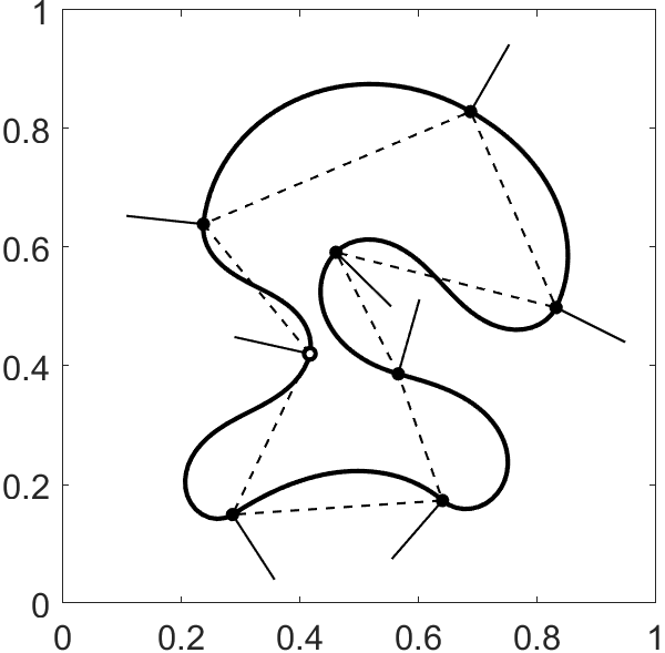
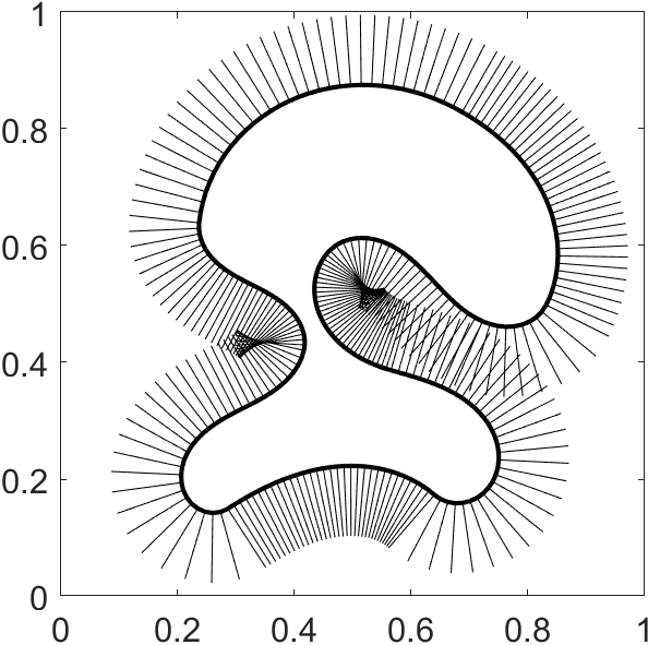
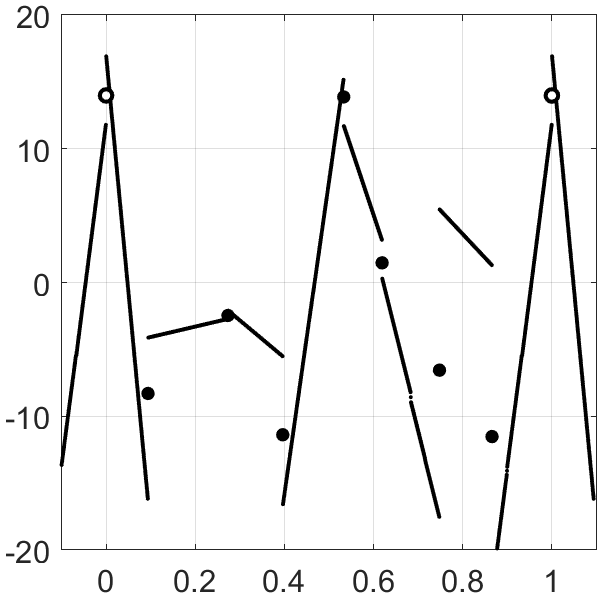
Figure 5: Lane-Riesenfeld-type subdivision of degree $n=1$.

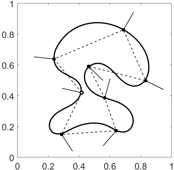
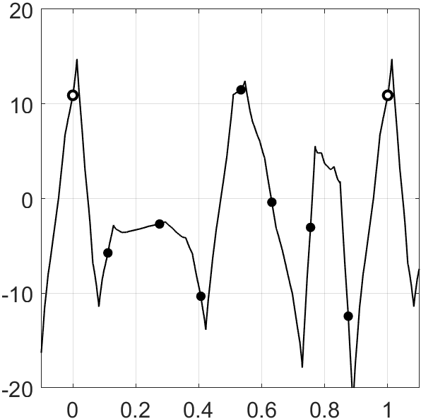
Figure 6: Lane-Riesenfeld-type subdivision of degree $n=2$.

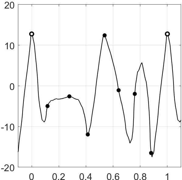
Figure 7: Lane-Riesenfeld-type subdivision of degree $n=3$.

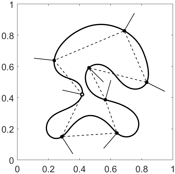
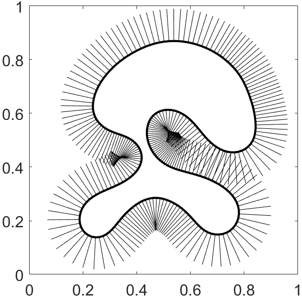
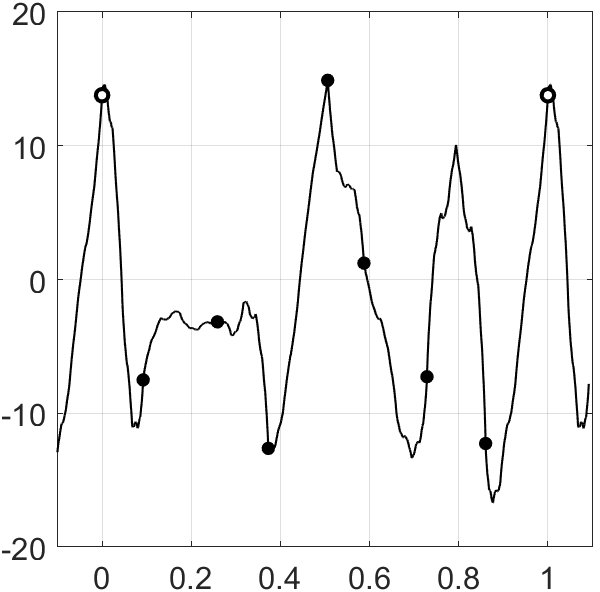
Figure 8: Four-point subdivision with weight $\omega=-1/18$.

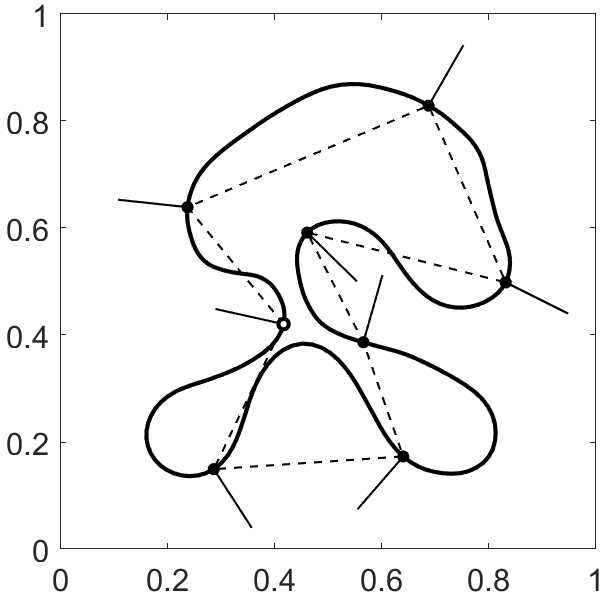
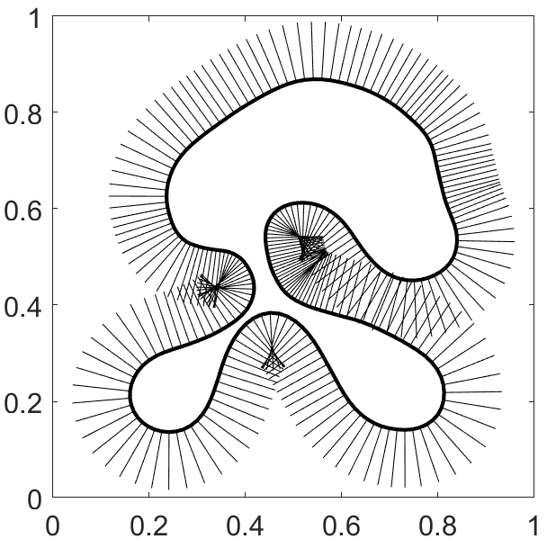
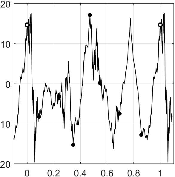
Figure 9: Four-point subdivision with weight $\omega=-1/9$.

6 $G^{1}$-convergence of the scheme $S_{1}$

While the focus of this paper is on the construction of geometric Hermite subdivision schemes, we also want to outline a proof for the $G^{1}$-convergence of the Lane-Riesenfeld-type algorithm $S_{1}$. It is based on the results in [DH12], but we want to remark that the notion of $G^{1}$ used there is special. It would be good to have a link between the approach of Dyn/Hormann and standard theory, which calls a curve $G^{1}$ if it has a $C^{1}$-reparametrization.

Convergence and smoothness are local properties of $S_{1}$ in the sense that the Hermite couples $h^{\ell}_{j}$ depend only on $h^{0}_{k},h^{0}_{k+1}$ for $k\leq j2^{-\ell}\leq k+1$, corresponding to the interval $[k,k+1]$ of the standard parametrization. That is, convergence and smoothness can be studied for initial data $H^{0}$ which are periodic in the sense that $h^{0}_{j}=h^{0}_{j+k},j\in\mathbb{Z}$, for some $k\geq 2$. This assumption avoids technical problems with unboundedness of sequences. Throughout, as before, $H^{\ell}=(h^{\ell}_{j})_{j\in\mathbb{Z}},h^{\ell}_{j}=(p^{\ell}_{j},\alpha^{\ell}_{j})$. Further, we define the vectors $d^{\ell}_{j}:=p^{\ell}_{j+1}-p^{\ell}_{j}$ and the pairs of angles $\beta^{\ell}_{j,J}=(\beta^{\ell}_{j,0},\beta^{\ell}_{j,1})$ by

$$\beta^{\ell}_{j,0}:=\alpha^{\ell}_{j}-\arg d^{\ell}_{j},\quad\beta^{\ell}_{j,1}:=\alpha^{\ell}_{j+1}-\arg d^{\ell}_{j}.$$

The Euclidean disk in $\mathbb{R}^{2}$ with radius $3\pi/4$ is denoted by $B^{*}:=\{\beta_{J}:\|\beta_{J}\|_{2}\leq 3\pi/4\}$.

Theorem 6.1

Let $H^{0}$ be periodic. If $d^{0}_{j}\neq 0$ and $\beta^{0}_{j,J}\in B^{*}$ for all $j\in\mathbb{Z}$, then the iterates $H^{\ell}:=S_{1}^{\ell}H^{0}$ define a sequence of polygons $(p^{\ell}_{j})_{j\in\mathbb{Z}}$ converging to a $G^{1}$-limit in the sense of [DH12]. Moreover, the angles $\alpha^{\ell}_{j}$ converge to the arguments of $d^{\ell}_{j}$,

$$\lim_{\ell\to\infty}\max_{j\in\mathbb{Z}}\bigl{(}\alpha^{\ell}_{j}-\arg(d^{\ell}_{j})\bigr{)}=0.$$

Proof. We consider the two-point problem in normal position, $h_{0}=(0,\beta_{0}),h_{1}=(1,\beta_{1})$, with secant $d=1-0=1$ and angles $(\beta_{0},\beta_{1})\in B^{*}$. The clothoid average

$$h_{1/2}=(p_{1/2},\alpha_{1/2}):=\frac{1}{2}h_{0}\oplus\frac{1}{2}h_{1}$$

yields new secants $d^{\prime}_{0}=p_{1/2},d^{\prime}_{1}=1-p_{1/2}$ and new pairs of angles

$$\beta^{\prime}_{0,J}=(\beta_{0}-\arg d^{\prime}_{0},\alpha_{1/2}-\arg d^{\prime}_{0}),\quad\beta^{\prime}_{1,J}=(\alpha_{1/2}-\arg d^{\prime}_{1},\beta_{1}-\arg d^{\prime}_{1}).$$

Figure 10 shows that the ratios

$$r(\beta):=\frac{\max\bigl{\{}|d^{\prime}_{0}|,|d^{\prime}_{1}|\bigr{\}}}{|d|},\quad\rho(\beta):=\frac{\max\bigl{\{}\|\beta^{\prime}_{0,J}\|_{2},\|\beta^{\prime}_{1,J}\|_{2}\bigr{\}}}{\|\beta_{J}\|_{2}},\quad\beta\in B^{*},$$

are bounded by $\|r\|_{\infty}\leq 4/5$ and $\|\rho\|_{\infty}\leq 19/20$, respectively. Now, consider a pair of consecutive Hermite couples $h^{\ell-1}_{j},h^{\ell-1}_{j+1}$ and its two descendants. The ratios

$$r^{\ell}_{j}:=\frac{\max\bigl{\{}|d^{\ell}_{2j}|,|d^{\ell}_{2j+1}|\bigr{\}}}{|d^{\ell-1}_{j}|},\quad\rho^{\ell}_{j}:=\frac{\max\bigl{\{}\|\beta^{\ell}_{2j,J}\|_{2},\|\beta^{\ell}_{2j+1,J}\|_{2}\bigr{\}}}{\|\beta^{\ell-1}_{j,J}\|_{2}}$$

are invariant under similarities so that we may move the configuration to normal position, showing that $r^{\ell}_{j}\leq\|r\|_{\infty}\leq 4/5$ and $\rho^{\ell}_{j}\leq\|\rho\|_{\infty}\leq 19/20$. The latter bound guarantees that $\beta^{\ell}_{j,J}\in B^{*}$ for all $j\in\mathbb{Z}$ and $\ell\in\mathbb{N}$. Taking the maximum over all elements at level $\ell$ and iterating backwards, we obtain

$$\max_{j}|d^{\ell}_{j}|\leq(4/5)^{\ell}\max_{j}|d^{0}_{j}|,\quad\max_{j}\|\beta^{\ell}_{j,J}\|_{2}\leq(19/20)^{\ell}\max_{j}\|\beta^{0}_{j,J}\|_{2}.$$

First, the sequence of maximal secant lengths is summable, implying that the sequence of polygons $(p^{\ell}_{j})_{j\in\mathbb{Z}}$, converges to a continuous limit, see Theorem 3 and Proposition 4 in [DH12]. Second, to address $G^{1}$-continuity, we consider the exterior angles

$$\delta^{\ell}_{j}:=\arg(d^{\ell}_{j})-\arg(d^{\ell}_{j-1})=\beta^{\ell}_{j-1,1}-\beta^{\ell}_{j,0}$$

between consecutive secants. They are bounded by

$$\max_{j\in\mathbb{Z}}|\delta^{\ell}_{j}|\leq 2\max_{j\in\mathbb{Z}}\|\beta^{\ell}_{j,J}\|_{2}\leq 2\cdot(19/20)^{\ell}\max_{j\in\mathbb{Z}}\|\beta^{0}_{j,J}\|_{2}.$$

Hence, also the sequence of maximal exterior angles is summable, implying that the limit curve is $G^{1}$, see Theorem 18 in [DH12]. Third, the final statement of the theorem is a simple consequence of $\alpha^{\ell}_{j}-\arg(d^{\ell}_{j})=\beta^{\ell}_{j,0}$.

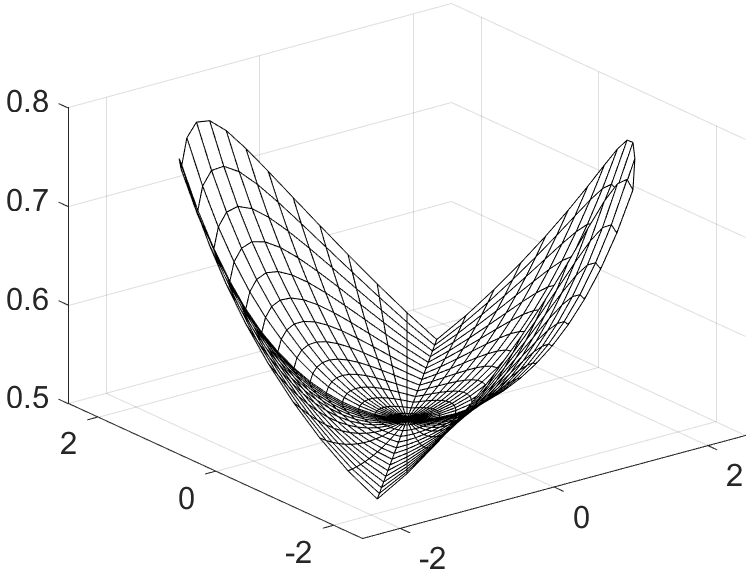
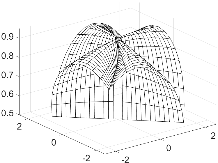
Figure 10: Contraction rates for lengths (left) and angles (right).

$\square$

7 Conclusion and Outlook

In this paper, we have proposed geometric Hermite subdivision schemes and we have demonstrated that they are a reasonable means for designing curves with prescribed tangents or normals. More precisely, we have first proposed an explicit strategy to approximate Hermite interpolating clothoids and used it to define the clothoid averages. Then we have used clothoidal averaging to define geometric Hermite subdivision schemes. Particular instances considered were the geometric Hermite analogues of the Lane-Riesenfeld schemes and of the four-point scheme. Examples demonstrate that these schemes yield very convincing results. Finally, we have presented some first smoothness results. More precisely, we obtain smoothness in the sense of [DH12] for the first order geometric Lane-Riesenfeld Hermite scheme. However, the notion of [DH12] is not standard; standard theory calls a curve $G^{1}$ if it has a $C^{1}$ reparametrization. It would be desirable to obtain related $G^{1}$- or even $G^{2}$-smoothness results for wider classes of schemes. This is an interesting topic of ongoing research.

References

- [AEV03] Nicolas Aspert, Touradj Ebrahimi, and Pierre Vandergheynst. Non-linear subdivision using local spherical coordinates. Computer Aided Geometric Design, 20(3):165–187, 2003.
- [AGRA15] Chebly Alia, Tagne Gilles, Talj Reine, and Charara Ali. Local trajectory planning and tracking of autonomous vehicles, using clothoid tentacles method. In 2015 IEEE Intelligent Vehicles Symposium (IV), pages 674–679. IEEE, 2015.
- [Baa84] K.G. Baass. The use of clothoid templates in highway design. Transportation Forum, 1:47–52, 1984.
- [BdB65] Garrett Birkhoff and Carl de Boor. Nonlinear splines. In Proc. General Motors Symp. of 1964, page 164–190. 1965.
- [Ber15] Matthew Berkemeier. Clothoid segments for optimal switching between arcs during low-speed Ackerman path tracking with rate-limited steering. In 2015 American Control Conference (ACC), pages 501–506. IEEE, 2015.
- [BF15] Enrico Bertolazzi and Marco Frego. fitting with clothoids. Mathematical Methods in the Applied Sciences, 38(5):881–897, 2015.
- [BF18] Enrico Bertolazzi and Marco Frego. Interpolating clothoid splines with curvature continuity. Mathematical Methods in the Applied Sciences, 41(4):1723–1737, 2018.
- [BL15] Budianto and Daniel Lun. Inpainting for fringe projection profilometry based on geometrically guided iterative regularization. IEEE Transactions on Image Processing, 24(12):5531–5542, 2015.
- [BLP10] Ilya Baran, Jaakko Lehtinen, and Jovan Popović. Sketching clothoid splines using shortest paths. In Computer Graphics Forum, volume 29, pages 655–664. Wiley Online Library, 2010.
- [BLR+12] Francesco Biral, Roberto Lot, Stefano Rota, Marco Fontana, and Véronique Huth. Intersection support system for powered two-wheeled vehicles: Threat assessment based on a receding horizon approach. IEEE Transactions on Intelligent Transportation Systems, 13(2):805–816, 2012.
- [CDM91] Alfred Cavaretta, Wolfgang Dahmen, and Charles Micchelli. Stationary subdivision, volume 453. American Mathematical Soc., 1991.
- [CDM03] Albert Cohen, Nira Dyn, and Basarab Matei. Quasilinear subdivision schemes with applications to ENO interpolation. Applied and Computational Harmonic Analysis, 15(2):89–116, 2003.
- [CHR13] Thomas Cashman, Kai Hormann, and Ulrich Reif. Generalized Lane–Riesenfeld algorithms. Computer Aided Geometric Design, 30(4):398–409, 2013.
- [CJ07] Pavel Chalmoviansky and Bert Jüttler. A non-linear circle-preserving subdivision scheme. Advances in Computational Mathematics, 27(4):375–400, 2007.
- [Coo93] Ian Coope. Curve interpolation with nonlinear spiral splines. IMA Journal of Numerical Analysis, 13(3):327–341, 1993.
- [DFH09] Nira Dyn, Michael Floater, and Kai Hormann. Four-point curve subdivision based on iterated chordal and centripetal parameterizations. Computer Aided Geometric Design, 26(3):279–286, 2009.
- [DH12] Nira Dyn and Kai Hormann. Geometric conditions for tangent continuity of interpolatory planar subdivision curves. Computer Aided Geometric Design, 29(6):332–347, 2012.
- [DL02] Nira Dyn and David Levin. Subdivision schemes in geometric modelling. Acta Numerica, 11:73–144, 2002.
- [DY00] David Donoho and Thomas Yu. Nonlinear pyramid transforms based on median-interpolation. SIAM Journal on Mathematical Analysis, 31(5):1030–1061, 2000.
- [ERS15] Tobias Ewald, Ulrich Reif, and Malcolm Sabin. Hölder regularity of geometric subdivision schemes. Constructive Approximation, 42(3):425–458, 2015.
- [Gro10] Philipp Grohs. A general proximity analysis of nonlinear subdivision schemes. SIAM Journal on Mathematical Analysis, 42(2):729–750, 2010.
- [GVS09] Ron Goldman, Etienne Vouga, and Scott Schaefer. On the smoothness of real-valued functions generated by subdivision schemes using nonlinear binary averaging. Computer Aided Geometric Design, 26:231–242, 2009.
- [Han18] Bin Han. Framelets and wavelets: Algorithms, analysis, and applications. Springer, 2018.
- [HEWF13] Sven Havemann, Johannes Edelsbrunner, Philipp Wagner, and Dieter Fellner. Curvature-controlled curve editing using piecewise clothoid curves. Computers & graphics, 37(6):764–773, 2013.
- [HL92] Josef Hoschek and Dieter Lasser. Grundlagen der geometrischen Datenverarbeitung. Teubner, 1992.
- [KFP03] Benjamin Kimia, Ilana Frankel, and Ana-Maria Popescu. Euler spiral for shape completion. International Journal of Computer Vision, 54(1-3):159–182, 2003.
- [KVD02] Frans Kuijt and Ruud Van Damme. Shape preserving interpolatory subdivision schemes for nonuniform data. Journal of Approximation Theory, 114(1):1–32, 2002.
- [LD16] Evgeny Lipovetsky and Nira Dyn. A weighted binary average of point-normal pairs with application to subdivision schemes. Computer Aided Geometric Design, 48:36–48, 2016.
- [MDL05] Martin Marinov, Nira Dyn, and David Levin. Geometrically controlled 4-point interpolatory schemes. In Advances in multiresolution for geometric modelling, pages 301–315. Springer, 2005.
- [Meh74] Even Mehlum. Nonlinear splines. In Computer Aided Geometric Design, pages 173–207. Elsevier, 1974.
- [Moo16] Caroline Moosmüller. Analysis of Hermite subdivision schemes on manifolds. SIAM Journal on Numerical Analysis, 54(5):3003–3031, 2016.
- [MS09] James McCrae and Karan Singh. Sketching piecewise clothoid curves. Computers & Graphics, 33(4):452–461, 2009.
- [MW90] Dereck Meek and Desmond Walton. Offset curves of clothoidal splines. Computer-Aided Design, 22(4):199–201, 1990.
- [MW92] Dereck Meek and Desmond Walton. Clothoid spline transition spirals. Mathematics of Computation, 59(199):117–133, 1992.
- [MW04] Dereck Meek and Desmond Walton. An arc spline approximation to a clothoid. Journal of Computational and Applied Mathematics, 170(1):59–77, 2004.
- [MW09] Dereck Meek and Desmond Walton. A two-point Hermite interpolating family of spirals. Journal of Computational and Applied Mathematics, 223(1):97–113, 2009.
- [PR08] Jörg Peters and Ulrich Reif. Subdivision surfaces. Springer, 2008.
- [SD04] Malcolm Sabin and Neil Dodgson. A circle-preserving variant of the four-point subdivision scheme. Mathematical Methods for Curves and Surfaces: Tromsø, pages 275–286, 2004.
- [SK00] Robert Schneider and Leif Kobbelt. Discrete fairing of curves and surfaces based on linear curvature distribution. In Curve and Surface Design, Saint-Malo 1999, Innovations in Applied Mathematics, pages 371–380, 2000.
- [Sto82] Josef Stoer. Curve fitting with clothoidal splines. J. Res. Nat. Bur. Standards, 87(4):317–346, 1982.
- [WD05] Johannes Wallner and Nira Dyn. Convergence and analysis of subdivision schemes on manifolds by proximity. Computer Aided Geometric Design, 22(7):593–622, 2005.
- [Wei10] Andreas Weinmann. Nonlinear subdivision schemes on irregular meshes. Constructive Approximation, 31(3):395–415, 2010.
- [WM09] Desmond Walton and Dereck Meek. interpolation with a single Cornu spiral segment. Journal of Computational and Applied Mathematics, 223(1):86 – 96, 2009.
- [XY09] Gang Xie and Thomas Yu. Smoothness equivalence properties of general manifold-valued data subdivision schemes. Multiscale Modeling & Simulation, 7(3):1073–1100, 2009.