Stability problem of equilibrium discrete planar curves

Yoshiki Jikumaru 111 Key words and phrases: discrete planar curve, variational problem, discrete curvature, Steiner formula, stability
Abstract

In this paper, we study planar polygonal curves from the variational methods. We show an unified interpretation of discrete curvatures and the Steiner-type formula by extracting the notion of the discrete curvature vector from the first variation of the length functional. Moreover, we determine the equilibrium curves for the length functional under the area-constraint condition and study their stability.

1 Introduction

Discrete differential geometry is an active research field in connection with the smooth manifold theory and the visualization on the computer. In this field, from the theoretical point of view, one approach is based on the variational problems and the other is the integrability of equations. We take the former approach and focus on discrete planar curves. Surprisingly, such a discrete curve theory is not well-understood, therefore we try to develop them inspired by the work [10]. Moreover, we consider the stability problem for equilibrium discrete curves. Stability problem for discrete objects have not developed well after the work by Polthier and Rossman [11].

First we derive the first variation formula and extract the vector from the formula which should be called the “discrete curvature vector” in §2. In §3, by using this curvature vector, we show an unifed interpretation which derives various kinds of discrete curvature notions introduced in [7], [8]. The important viewpoint here is that there is no natural notion of the line element on the vertices. In §4, we characterize equilibrium curves for the length functional under the area-constraint condition as regular polygons. In §5, we derive the Steiner-type formula for parallel curves by using the “vertex normal” constructed from the “discrete curvature vector” derived in §2. In §6, we will consider the stability problem of the regular polygons. We can derive the second variation formula similar to the smooth case by decomposing the variation vector field to the “normal” and “tangential” directions as in [1]. Moreover, we show the instability for the non-convex regular polygons by using the second variation formula for “normal” variations in the section 7.

2 The first variation formula

In this section we will consider the variation of discrete curves and extract the “curvature vector” from the first variation formula. We can expect that this vector gives a notion of the curvature and normal at vertices. Let us recall the basic definition of discrete planar curves.

Definition 2.1.

Let n𝑛n be a non-negative integer. A standard (abstract) n𝑛n-path is a simplicial complex G=(V,E)𝐺𝑉𝐸G=(V,E) formed by

  1. (1)1(1)

    (n+1)𝑛1(n+1) abstract points : V={v0,,vn}𝑉subscript𝑣0subscript𝑣𝑛V=\{v_{0},\ldots,v_{n}\}.

  2. (2)2(2)

    the set of n𝑛n edges ek=[vk,vk+1]subscript𝑒𝑘subscript𝑣𝑘subscript𝑣𝑘1e_{k}=[v_{k},v_{k+1}], k=0,,n1𝑘0𝑛1k=0,\ldots,n-1.

An standard abstract n𝑛n-circle is the union of a standard n𝑛n-path and the “final” edge en=[vn,v0]subscript𝑒𝑛subscript𝑣𝑛subscript𝑣0e_{n}=[v_{n},v_{0}]. A discrete (planar) curve is a geometric realization of a standard (n1)𝑛1(n-1)-path or (n1)𝑛1(n-1)-circle which is a map X:V2:𝑋𝑉superscript2X:V\to\mathbb{R}^{2} satisfies lk:=|pk+1pk|0assignsubscript𝑙𝑘subscript𝑝𝑘1subscript𝑝𝑘0l_{k}:=|p_{k+1}-p_{k}|\neq 0 for all k=0,1,,n1𝑘01𝑛1k=0,1,\ldots,n-1, where we denote pk:=X(vk)assignsubscript𝑝𝑘𝑋subscript𝑣𝑘p_{k}:=X(v_{k}). We denote such a discrete curve as Γh={pk}ksubscriptΓsubscriptsubscript𝑝𝑘𝑘\Gamma_{h}=\{p_{k}\}_{k}.

For each oriented edge ek:=[pk,pk+1]assignsubscript𝑒𝑘subscript𝑝𝑘subscript𝑝𝑘1e_{k}:=[p_{k},p_{k+1}] of ΓhsubscriptΓ\Gamma_{h} we can assign an unit normal vector

νk:=R(pk+1pklk):=R(pk+1pk|pk+1pk|),k=0,,n1,formulae-sequenceassignsubscript𝜈𝑘𝑅subscript𝑝𝑘1subscript𝑝𝑘subscript𝑙𝑘assign𝑅subscript𝑝𝑘1subscript𝑝𝑘subscript𝑝𝑘1subscript𝑝𝑘𝑘0𝑛1\nu_{k}:=R\left(\frac{p_{k+1}-p_{k}}{l_{k}}\right):=R\left(\frac{p_{k+1}-p_{k}}{|p_{k+1}-p_{k}|}\right),\quad k=0,\ldots,n-1,

where R𝑅R is the π/2𝜋2\pi/2-rotation or π/2𝜋2-\pi/2-rotation in 2superscript2\mathbb{R}^{2}. It does not matter whichever we choose but we choose the same R𝑅R for all k𝑘k.

For a discrete curve Γh={pk}ksubscriptΓsubscriptsubscript𝑝𝑘𝑘\Gamma_{h}=\{p_{k}\}_{k} with an orientation, the length of ΓhsubscriptΓ\Gamma_{h} and the 222-dimensional volume (area) bounded by ΓhsubscriptΓ\Gamma_{h} are defined by

L(Γh):=klk=k|pk+1pk|,Vol(Γh):= 12kpk,νk|pk+1pk|formulae-sequenceassign𝐿subscriptΓsubscript𝑘subscript𝑙𝑘subscript𝑘subscript𝑝𝑘1subscript𝑝𝑘assignVolsubscriptΓ12subscript𝑘subscript𝑝𝑘subscript𝜈𝑘subscript𝑝𝑘1subscript𝑝𝑘L(\Gamma_{h}):=\sum_{k}l_{k}=\sum_{k}|p_{k+1}-p_{k}|,\quad\operatorname{Vol}(\Gamma_{h}):=\frac{\,1\,}{2}\sum_{k}\langle p_{k},\nu_{k}\rangle|p_{k+1}-p_{k}|

In these settings, we consider the following question:

What is the unit normal, curvature and line element at the vertices ?

A realization of the dual graph may give an answer for this question, but we do not consider such a realization. In order to approach the problem, we will extract the discrete curvature vector from the first variation of the length. Therefore we first derive the first variation formula of the length functional. In the discrete setting we consider the variation of vertices, that is, piecewise linear variations. We consider a variation

pk(t)=pk+tvk+O(t2),k=0,,n1formulae-sequencesubscript𝑝𝑘𝑡subscript𝑝𝑘𝑡subscript𝑣𝑘𝑂superscript𝑡2𝑘0𝑛1p_{k}(t)=p_{k}+tv_{k}+O(t^{2}),\quad k=0,\ldots,n-1

where vt=(v0t,,vn1t)2nsuperscript𝑣𝑡superscriptsubscript𝑣0𝑡superscriptsubscript𝑣𝑛1𝑡superscript2𝑛{}^{t}\vec{v}=({}^{t}v_{0},\ldots,{}^{t}v_{n-1})\in\mathbb{R}^{2n} is the “variation vector field”. If pksubscript𝑝𝑘p_{k} is a boundary point of ΓhsubscriptΓ\Gamma_{h}, then we assume vk=0subscript𝑣𝑘0v_{k}=0.

We want to find the vector tL2n{}^{t}\nabla L\in\mathbb{R}^{2n} satisfies

δL:=ddt|t=0L=v,L2n=kvk,pkL2,\delta L:=\frac{d}{dt}_{|t=0}L=\langle\vec{v},\nabla L\rangle_{\mathbb{R}^{2n}}=\sum_{k}\langle v_{k},\nabla_{p_{k}}L\rangle_{\mathbb{R}^{2}},

where we write tL=(p1tL,,pntL)2n{}^{t}\nabla L=({}^{t}\nabla_{p_{1}}L,\ldots,{}^{t}\nabla_{p_{n}}L)\in\mathbb{R}^{2n}. Since this is just a direction derivative in 2nsuperscript2𝑛\mathbb{R}^{2n}, the following proposition is immediately:

Proposition 2.2.

Let Γh={pk}ksubscriptΓsubscriptsubscript𝑝𝑘𝑘\Gamma_{h}=\{p_{k}\}_{k} be a discrete closed curve and pksubscript𝑝𝑘p_{k} be an interior vertex. Then the gradient the length can be expressed in the following formula:

pkL=R(νkνk1)=pk+1pklk+pkpk1lk1.subscriptsubscript𝑝𝑘𝐿𝑅subscript𝜈𝑘subscript𝜈𝑘1subscript𝑝𝑘1subscript𝑝𝑘subscript𝑙𝑘subscript𝑝𝑘subscript𝑝𝑘1subscript𝑙𝑘1\nabla_{p_{k}}L=R(\nu_{k}-\nu_{k-1})=-\frac{p_{k+1}-p_{k}}{l_{k}}+\frac{p_{k}-p_{k-1}}{l_{k-1}}. (2.1)

By using this formula we have

δL=kpkL,vk=k 1LkpkL,vkLk,𝛿𝐿subscript𝑘subscriptsubscript𝑝𝑘𝐿subscript𝑣𝑘subscript𝑘1subscript𝐿𝑘subscriptsubscript𝑝𝑘𝐿subscript𝑣𝑘subscript𝐿𝑘\delta L=\sum_{k}\langle\nabla_{p_{k}}L,v_{k}\rangle=-\sum_{k}\left\langle-\frac{\,1\,}{L_{k}}\nabla_{p_{k}}L,v_{k}\right\rangle L_{k},

where we inserted some auxilary function Lksubscript𝐿𝑘L_{k} defined on the vertices. This kind of observation is essentially remarked in the paper [3].

Definition 2.3 (Discrete curvature vector).

For a positive function Lksubscript𝐿𝑘L_{k} defined on the vertices, we call the vector

N~k= 1LkpkL= 1Lk(pk+1pklkpkpk1lk1)subscript~𝑁𝑘1subscript𝐿𝑘subscriptsubscript𝑝𝑘𝐿1subscript𝐿𝑘subscript𝑝𝑘1subscript𝑝𝑘subscript𝑙𝑘subscript𝑝𝑘subscript𝑝𝑘1subscript𝑙𝑘1\widetilde{N}_{k}=-\frac{\,1\,}{L_{k}}\nabla_{p_{k}}L=\frac{\,1\,}{L_{k}}\left(\frac{p_{k+1}-p_{k}}{l_{k}}-\frac{p_{k}-p_{k-1}}{l_{k-1}}\right) (2.2)

the discrete curvature vector with respect to Lksubscript𝐿𝑘L_{k}.

Remarks .

There are some reasons why we can regard the vector N~ksubscript~𝑁𝑘\widetilde{N}_{k} as the curvature vector. First, the vector N~ksubscript~𝑁𝑘\widetilde{N}_{k} is independent of the choice of the unit normal, i.e., an intrinsic quantity. Moreover, the second expression (2.2) can be regarded as a discretization of a part of the Frenet-Serret formula. As we will remark below, suitable choices of the function Lksubscript𝐿𝑘L_{k} derives various notions of discrete curvature defined in [7], [8]. Non-uniqueness of the function Lksubscript𝐿𝑘L_{k} comes from the fact that there is no natural line element, i.e. the metric, at vertices.

3 Relation with other notions of the discrete curvature

In this section, non-uniqueness of the line element at the vertices gives various notions of the discrete curvature defined in [7], [8].

To describe the curvature notions, we have to define the angles at vertices. We define (the absolute value of) the angle between νk1subscript𝜈𝑘1\nu_{k-1} and νksubscript𝜈𝑘\nu_{k} as θksubscript𝜃𝑘\theta_{k}, i.e.,

cosθk:=νk,νk1=pk+1pk,pkpk1|pk+1pk||pkpk1|.assignsubscript𝜃𝑘subscript𝜈𝑘subscript𝜈𝑘1subscript𝑝𝑘1subscript𝑝𝑘subscript𝑝𝑘subscript𝑝𝑘1subscript𝑝𝑘1subscript𝑝𝑘subscript𝑝𝑘subscript𝑝𝑘1\cos\theta_{k}:=\langle\nu_{k},\nu_{k-1}\rangle=\frac{\langle p_{k+1}-p_{k},p_{k}-p_{k-1}\rangle}{|p_{k+1}-p_{k}|\cdot|p_{k}-p_{k-1}|}.

We have to care about the signature of θksubscript𝜃𝑘\theta_{k}. Let Rθsubscript𝑅𝜃R_{\theta} be the θ𝜃\theta-rotation in 2superscript2\mathbb{R}^{2}. We assign the signature depends on the choice of the rotation R𝑅R appeared in the definition of the edge normal:

σ:={+1ifR=Rπ/21ifR=Rπ/2assign𝜎cases1if𝑅subscript𝑅𝜋21if𝑅subscript𝑅𝜋2\sigma:=\begin{cases}+1\quad&{\rm if}\quad R=R_{\pi/2}\\ -1\quad&{\rm if}\quad R=R_{-\pi/2}\end{cases}

In this situation the signature of θksubscript𝜃𝑘\theta_{k} is determined by the equation Rσθk(νk1)=νksubscript𝑅𝜎subscript𝜃𝑘subscript𝜈𝑘1subscript𝜈𝑘R_{\sigma\theta_{k}}(\nu_{k-1})=\nu_{k}. We easily see that kθk=2mπsubscript𝑘subscript𝜃𝑘2𝑚𝜋\sum_{k}\theta_{k}=2m\pi for some integer m𝑚m\in\mathbb{Z} for any closed curve. We define the discrete curvature with respect to the choice of Lksubscript𝐿𝑘L_{k} by the length of the discrete curvature vector with respect to Lksubscript𝐿𝑘L_{k}:

Definition 3.1.

For a positive function Lksubscript𝐿𝑘L_{k} defined on the vertices, we call the value

κ(pk):=2sin(θk/2)Lkassign𝜅subscript𝑝𝑘2subscript𝜃𝑘2subscript𝐿𝑘\kappa(p_{k}):=\frac{2\sin(\theta_{k}/2)}{L_{k}}

the discrete curvature with respect to Lksubscript𝐿𝑘L_{k}.

Remark .

If we use the expression pk=R(νkνk1)subscriptsubscript𝑝𝑘𝑅subscript𝜈𝑘subscript𝜈𝑘1\nabla_{p_{k}}=R(\nu_{k}-\nu_{k-1}), the discrete curvature with respect to Lksubscript𝐿𝑘L_{k} can be written as κ(pk)=|νkνk1|/Lk𝜅subscript𝑝𝑘subscript𝜈𝑘subscript𝜈𝑘1subscript𝐿𝑘\kappa(p_{k})=|\nu_{k}-\nu_{k-1}|/L_{k} up to the signature. This can be regarded as a discretization of the curvature for a regular planar curve.

In the lecture note by Tim Hoffmann [8], three kinds of notions of the curvature for discrete curves are introduced:

  1. (1)1(1)

    The curvature at vertices by using the vertex osculating circle method,

  2. (2)2(2)

    The curvature at edges by using the edge osculating circle method,

  3. (3)3(3)

    The curvature at vertices by using edge osculating circle for “arclength parametrized” curve.

Moreover, Hatakeyama [7] also defined the curvature for discrete curves another way. We will show that these curvature notions can be derived from our viewpoint.

Proposition 3.2 (The vertex osculating circle method [8]).

If we choose

Lk=|pk+1pk1|2cos(θk/2)=|pk+1pk+pkpk1|2cos(θk/2),subscript𝐿𝑘subscript𝑝𝑘1subscript𝑝𝑘12subscript𝜃𝑘2subscript𝑝𝑘1subscript𝑝𝑘subscript𝑝𝑘subscript𝑝𝑘12subscript𝜃𝑘2L_{k}=\frac{|p_{k+1}-p_{k-1}|}{2\cos(\theta_{k}/2)}=\frac{|p_{k+1}-p_{k}+p_{k}-p_{k-1}|}{2\cos(\theta_{k}/2)},

then the discrete curvature with respect to Lksubscript𝐿𝑘L_{k} becomes

κ(pk)=2sinθk|pk+1pk1|=2sinθk|pk+1pk+pkpk1|𝜅subscript𝑝𝑘2subscript𝜃𝑘subscript𝑝𝑘1subscript𝑝𝑘12subscript𝜃𝑘subscript𝑝𝑘1subscript𝑝𝑘subscript𝑝𝑘subscript𝑝𝑘1\kappa(p_{k})=\frac{2\sin\theta_{k}}{|p_{k+1}-p_{k-1}|}=\frac{2\sin\theta_{k}}{|p_{k+1}-p_{k}+p_{k}-p_{k-1}|}

and this value coincides with the curvature based on the vertex osculating circle method.

Proposition 3.3 (For the arclength parametrized curves [8]).

Assume lk=lk1=l0subscript𝑙𝑘subscript𝑙𝑘1subscript𝑙0l_{k}=l_{k-1}=l_{0}. Then if we choose

Lk=l0cosθk2=lk+lk12cosθk2,subscript𝐿𝑘subscript𝑙0subscript𝜃𝑘2subscript𝑙𝑘subscript𝑙𝑘12subscript𝜃𝑘2L_{k}=l_{0}\cos\frac{\theta_{k}}{2}=\frac{l_{k}+l_{k-1}}{2}\cdot\cos\frac{\theta_{k}}{2},

then the discrete curvature with respect to Lksubscript𝐿𝑘L_{k} becomes

κ(pk)=2l0tanθk2𝜅subscript𝑝𝑘2subscript𝑙0subscript𝜃𝑘2\kappa(p_{k})=\frac{2}{l_{0}}\tan\frac{\theta_{k}}{2}

and this value coincides with the curvature of arclength parametrized curve.

In the paper [7], the discrete curvature at the vertex is defined as

κ(pk):=1|pkpk1||pk+1pk|pk+1pk|pkpk1|pkpk1||=|pkL||pkpk1|.assign𝜅subscript𝑝𝑘1subscript𝑝𝑘subscript𝑝𝑘1subscript𝑝𝑘1subscript𝑝𝑘subscript𝑝𝑘1subscript𝑝𝑘subscript𝑝𝑘subscript𝑝𝑘1subscript𝑝𝑘subscript𝑝𝑘1subscriptsubscript𝑝𝑘𝐿subscript𝑝𝑘subscript𝑝𝑘1\kappa(p_{k}):=\frac{1}{|p_{k}-p_{k-1}|}\left|\frac{p_{k+1}-p_{k}}{|p_{k+1}-p_{k}|}-\frac{p_{k}-p_{k-1}}{|p_{k}-p_{k-1}|}\right|=-\frac{|\nabla_{p_{k}}L|}{|p_{k}-p_{k-1}|}.

Then we immediately have the following result:

Proposition 3.4.

If we choose Lk=lk1=|pkpk1|subscript𝐿𝑘subscript𝑙𝑘1subscript𝑝𝑘subscript𝑝𝑘1L_{k}=l_{k-1}=|p_{k}-p_{k-1}|, then the discrete curvature with respect to Lksubscript𝐿𝑘L_{k} coincides with the discrete curvature defined in [7].

Before considering the edge osculating circle method, we shall modify the first variation formula from the vertex-based expression to the edge-based expression. If we put vk=(wk+wk1)/2subscript𝑣𝑘subscript𝑤𝑘subscript𝑤𝑘12v_{k}=(w_{k}+w_{k-1})/2, then we have

δL𝛿𝐿\displaystyle\delta L =12kpkL,wk+wk1absent12subscript𝑘subscriptsubscript𝑝𝑘𝐿subscript𝑤𝑘subscript𝑤𝑘1\displaystyle=\frac{1}{2}\sum_{k}\langle\nabla_{p_{k}}L,w_{k}+w_{k-1}\rangle
=12kpkL+pk+1L,wk=kR(νk1νk+1)2Lk,wkLkabsent12subscript𝑘subscriptsubscript𝑝𝑘𝐿subscriptsubscript𝑝𝑘1𝐿subscript𝑤𝑘subscript𝑘𝑅subscript𝜈𝑘1subscript𝜈𝑘12superscriptsubscript𝐿𝑘subscript𝑤𝑘superscriptsubscript𝐿𝑘\displaystyle=\frac{1}{2}\sum_{k}\langle\nabla_{p_{k}}L+\nabla_{p_{k+1}}L,w_{k}\rangle=-\sum_{k}\left\langle\frac{R(\nu_{k-1}-\nu_{k+1})}{2L_{k}^{\prime}},w_{k}\right\rangle L_{k}^{\prime}

where Lksuperscriptsubscript𝐿𝑘L_{k}^{\prime} is some auxiliary function. As in the vertex case, we call the value

κ(ek):=1Lksinθk+θk+12assign𝜅subscript𝑒𝑘1superscriptsubscript𝐿𝑘subscript𝜃𝑘subscript𝜃𝑘12\kappa(e_{k}):=\frac{1}{L_{k}^{\prime}}\cdot\sin\frac{\theta_{k}+\theta_{k+1}}{2}

the discrete curvature at the edge ek=[pk,pk+1]subscript𝑒𝑘subscript𝑝𝑘subscript𝑝𝑘1e_{k}=[p_{k},p_{k+1}] with respect to Lksuperscriptsubscript𝐿𝑘L_{k}^{\prime}.

Proposition 3.5 (The edge osculating circle method [8]).

If we choose

Lk=lkcosθk2cosθk+12=|pk+1pk|cosθk2cosθk+12,superscriptsubscript𝐿𝑘subscript𝑙𝑘subscript𝜃𝑘2subscript𝜃𝑘12subscript𝑝𝑘1subscript𝑝𝑘subscript𝜃𝑘2subscript𝜃𝑘12L_{k}^{\prime}=l_{k}\cos\frac{\theta_{k}}{2}\cos\frac{\theta_{k+1}}{2}=|p_{k+1}-p_{k}|\cos\frac{\theta_{k}}{2}\cos\frac{\theta_{k+1}}{2},

then the discrete curvature with respect to Lksuperscriptsubscript𝐿𝑘L_{k}^{\prime} becomes

κ(ek)=tan(θk/2)+tan(θk+1/2)|pk+1pk|𝜅subscript𝑒𝑘subscript𝜃𝑘2subscript𝜃𝑘12subscript𝑝𝑘1subscript𝑝𝑘\kappa(e_{k})=\frac{\tan(\theta_{k}/2)+\tan(\theta_{k+1}/2)}{|p_{k+1}-p_{k}|}

and this value coincides with the curvature based on the edge osculating circle method.

Remark .

To define the discrete curvature, we have to choose Lksubscript𝐿𝑘L_{k} (respectively Lksuperscriptsubscript𝐿𝑘L_{k}^{\prime}) properly. That means if lksubscript𝑙𝑘l_{k}, lk1dssubscript𝑙𝑘1𝑑𝑠l_{k-1}\to ds and θk0subscript𝜃𝑘0\theta_{k}\to 0, then Lksubscript𝐿𝑘L_{k} (respectively Lksuperscriptsubscript𝐿𝑘L_{k}^{\prime}) must converge to ds𝑑𝑠ds, i.e., Lksubscript𝐿𝑘L_{k} must be a “good” candidate for a discrete line element. We can check that Lksubscript𝐿𝑘L_{k} and Lksuperscriptsubscript𝐿𝑘L_{k}^{\prime} satisfy this condition in the above examples.

Remark (“No free lunch” for the discrete Laplacian, cf. [12]).

We consider these kinds of “no free lunch” story for the discrete Laplacian which will be used in the second variation formula. On a discrete curve ΓhsubscriptΓ\Gamma_{h} with the vertex set V𝑉V, we consider a function ψ:V:𝜓𝑉\psi:V\to\mathbb{R}. Then the gradient and the Laplacian of ψ𝜓\psi can be defined as

ψk:=ψk+1ψklk,Δψk:=1Lk(ψkψk1)=1Lk(ψk+1ψklkψkψk1lk1),formulae-sequenceassignsubscript𝜓𝑘subscript𝜓𝑘1subscript𝜓𝑘subscript𝑙𝑘assignΔsubscript𝜓𝑘1subscript𝐿𝑘subscript𝜓𝑘subscript𝜓𝑘11subscript𝐿𝑘subscript𝜓𝑘1subscript𝜓𝑘subscript𝑙𝑘subscript𝜓𝑘subscript𝜓𝑘1subscript𝑙𝑘1\nabla\psi_{k}:=\frac{\psi_{k+1}-\psi_{k}}{l_{k}},\quad\Delta\psi_{k}:=\frac{1}{L_{k}}(\nabla\psi_{k}-\nabla\psi_{k-1})=\frac{1}{L_{k}}\left(\frac{\psi_{k+1}-\psi_{k}}{l_{k}}-\frac{\psi_{k}-\psi_{k-1}}{l_{k-1}}\right),

where we denote ψk:=ψ(k)assignsubscript𝜓𝑘𝜓𝑘\psi_{k}:=\psi(k). Note that the gradient is the “edge-based operator” but the Laplacian is the “vertex-based” operator. In addition, the discrete curvature vector N~ksubscript~𝑁𝑘\widetilde{N}_{k} with respect to Lksubscript𝐿𝑘L_{k} can be written as ΔpkΔsubscript𝑝𝑘\Delta p_{k}.

From another point of view, if we define the Dirichlet energy of ψ𝜓\psi as

Eh(ψ):=12k|ψk|2lk=12k|ψk+1ψk|2lk,assignsubscript𝐸𝜓12subscript𝑘superscriptsubscript𝜓𝑘2subscript𝑙𝑘12subscript𝑘superscriptsubscript𝜓𝑘1subscript𝜓𝑘2subscript𝑙𝑘E_{h}(\psi):=\frac{1}{2}\sum_{k}|\nabla\psi_{k}|^{2}\,l_{k}=\frac{1}{2}\sum_{k}\frac{|\psi_{k+1}-\psi_{k}|^{2}}{l_{k}},

then the first variation of the energy becomes

δEh(ψ)=kψk+1ψk,φk+1φklk=kψk1ψk,φk=kΔψk,φkLk,𝛿subscript𝐸𝜓subscript𝑘subscript𝜓𝑘1subscript𝜓𝑘subscript𝜑𝑘1subscript𝜑𝑘subscript𝑙𝑘subscript𝑘subscript𝜓𝑘1subscript𝜓𝑘subscript𝜑𝑘subscript𝑘Δsubscript𝜓𝑘subscript𝜑𝑘subscript𝐿𝑘\delta E_{h}(\psi)=\sum_{k}\frac{\langle\psi_{k+1}-\psi_{k},\varphi_{k+1}-\varphi_{k}\rangle}{l_{k}}=\sum_{k}\langle\nabla\psi_{k-1}-\nabla\psi_{k},\varphi_{k}\rangle=-\sum_{k}\langle\Delta\psi_{k},\varphi_{k}\rangle L_{k},

where we take the variation of ψ𝜓\psi as ψk(t)=ψk+tφk+O(t2)subscript𝜓𝑘𝑡subscript𝜓𝑘𝑡subscript𝜑𝑘𝑂superscript𝑡2\psi_{k}(t)=\psi_{k}+t\varphi_{k}+O(t^{2}). Therefore δEh(ψ)=0𝛿subscript𝐸𝜓0\delta E_{h}(\psi)=0 if and only if Δψk=0Δsubscript𝜓𝑘0\Delta\psi_{k}=0. Note that the condition Δψk=0Δsubscript𝜓𝑘0\Delta\psi_{k}=0 is independent of the choice of Lksubscript𝐿𝑘L_{k}.

As in the curvature case, the Laplacian can be changed since there is no natural “line element divisor Lksubscript𝐿𝑘L_{k}”. However, with another function φ:V:𝜑𝑉\varphi:V\to\mathbb{R}, we still have the following properties since the quanties ΔψkLkΔsubscript𝜓𝑘subscript𝐿𝑘\Delta\psi_{k}L_{k} are independent of Lksubscript𝐿𝑘L_{k}:

  1. (1)1(1)

    If ψ𝜓\psi is constant, then Δψ=0Δ𝜓0\Delta\psi=0.

  2. (2)2(2)

    The condition Δψ=0Δ𝜓0\Delta\psi=0 is independent of the choice of Lksubscript𝐿𝑘L_{k} and in this case we have the mean value property:

    ψk=lk1lk+lk1ψk+1+lklk+lk1ψk1.subscript𝜓𝑘subscript𝑙𝑘1subscript𝑙𝑘subscript𝑙𝑘1subscript𝜓𝑘1subscript𝑙𝑘subscript𝑙𝑘subscript𝑙𝑘1subscript𝜓𝑘1\psi_{k}=\frac{l_{k-1}}{l_{k}+l_{k-1}}\psi_{k+1}+\frac{l_{k}}{l_{k}+l_{k-1}}\psi_{k-1}.
  3. (3)3(3)

    L2superscript𝐿2L^{2} symmetric property:

    kψkΔφkLk=kΔψkφkLk.subscript𝑘subscript𝜓𝑘Δsubscript𝜑𝑘subscript𝐿𝑘subscript𝑘Δsubscript𝜓𝑘subscript𝜑𝑘subscript𝐿𝑘\sum_{k}\psi_{k}\cdot\Delta\varphi_{k}\cdot L_{k}=\sum_{k}\Delta\psi_{k}\cdot\varphi_{k}\cdot L_{k}.

    Note that the summation is vertex-based.

  4. (4)4(4)

    Integration by parts:

    kψkΔφkLk=kψkφklk.subscript𝑘subscript𝜓𝑘Δsubscript𝜑𝑘subscript𝐿𝑘subscript𝑘subscript𝜓𝑘subscript𝜑𝑘subscript𝑙𝑘-\sum_{k}\psi_{k}\cdot\Delta\varphi_{k}\cdot L_{k}=\sum_{k}\nabla\psi_{k}\cdot\nabla\varphi_{k}\cdot l_{k}.

    Note that the right hand side is the edge-based summation but the left hand side is the vertex-based summation. As a corollary, the operator ΔΔ-\Delta is positive semi-definite.

4 Equilibrium curves of the length functional

In the previous section, we showed that non-uniqueness of the line element at vertices gives various discrete curvature notions. However, the equilibrium curves for the length functional under the area-constraint condition should be characterized as some “constant curvature” objects by virture of the smooth case. In this section, we show that such equilibrium curves can be characterized as regular polygons and that they are certainly regarded as “constant curvature” objects.

By a direct calculation we have the following result.

Lemma 4.1.

For any vertex pksubscript𝑝𝑘p_{k} of ΓhsubscriptΓ\Gamma_{h} the gradient of the area pkVolsubscriptsubscript𝑝𝑘Vol\nabla_{p_{k}}\operatorname{Vol} is given by

pkVol=12R(pk+1pk1).subscriptsubscript𝑝𝑘Vol12𝑅subscript𝑝𝑘1subscript𝑝𝑘1\nabla_{p_{k}}\operatorname{Vol}=\frac{1}{2}R(p_{k+1}-p_{k-1}).
Remark (Another “no free lunch” story).

We can modify the first variation formula of the volume as follows:

δVol=12kR(pk+1pk+pkpk1),vk=klkνk+lk1νk12Lk,vkLk.𝛿Vol12subscript𝑘𝑅subscript𝑝𝑘1subscript𝑝𝑘subscript𝑝𝑘subscript𝑝𝑘1subscript𝑣𝑘subscript𝑘subscript𝑙𝑘subscript𝜈𝑘subscript𝑙𝑘1subscript𝜈𝑘12subscript𝐿𝑘subscript𝑣𝑘subscript𝐿𝑘\delta\operatorname{Vol}=\frac{1}{2}\sum_{k}\langle R(p_{k+1}-p_{k}+p_{k}-p_{k-1}),v_{k}\rangle=\sum_{k}\left\langle\frac{l_{k}\nu_{k}+l_{k-1}\nu_{k-1}}{2L_{k}},v_{k}\right\rangle L_{k}.

At a glance, it seems like a natural to choose 2Lk=lk+lk1=Length(star(p))2subscript𝐿𝑘subscript𝑙𝑘subscript𝑙𝑘1Lengthstar𝑝2L_{k}=l_{k}+l_{k-1}=\operatorname{Length}({\rm star}\,(p)) and this is also frequently used as a “vertex normal” (a weighted sum of the edge normals):

NkV:=lkνk+lk1νk1lk+lk1.assignsuperscriptsubscript𝑁𝑘𝑉subscript𝑙𝑘subscript𝜈𝑘subscript𝑙𝑘1subscript𝜈𝑘1subscript𝑙𝑘subscript𝑙𝑘1N_{k}^{V}:=\frac{l_{k}\nu_{k}+l_{k-1}\nu_{k-1}}{l_{k}+l_{k-1}}.

In addition, we have

pkL=R(νk1νk)=sinθk1+cosθk(νk+νk1)=2tanθk2νk+νk12.subscriptsubscript𝑝𝑘𝐿𝑅subscript𝜈𝑘1subscript𝜈𝑘subscript𝜃𝑘1subscript𝜃𝑘subscript𝜈𝑘subscript𝜈𝑘12subscript𝜃𝑘2subscript𝜈𝑘subscript𝜈𝑘12-\nabla_{p_{k}}L=R(\nu_{k-1}-\nu_{k})=\frac{\sin\theta_{k}}{1+\cos\theta_{k}}(\nu_{k}+\nu_{k-1})=2\tan\frac{\theta_{k}}{2}\cdot\frac{\nu_{k}+\nu_{k-1}}{2}.

by a simple calculation. Therefore, unless the curve is arclength parameterized, there are (at least) two choices of the “vertex normal” from the variational viewpoint: using the length gradient (length descent direction) or using the volume gradient (volume descent direction). This suggests that, in contrast to the smooth case, we have to choose the “prefered” vertex normal according to the energy in question. \Box

Example 4.2 (Regular polygons).

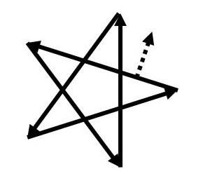
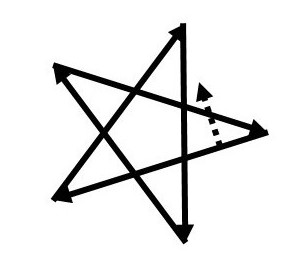
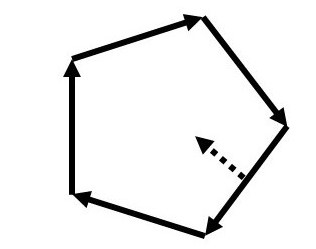
Let us take a discrete curve Γhm,n={pk}ksuperscriptsubscriptΓ𝑚𝑛subscriptsubscript𝑝𝑘𝑘\Gamma_{h}^{m,n}=\{p_{k}\}_{k} as in the following way (including non-convex regular n𝑛n-gon with radius a𝑎a):

pk=aexp(2π1mk/n),k=0,,n1,1mn1,formulae-sequencesubscript𝑝𝑘𝑎2𝜋1𝑚𝑘𝑛formulae-sequence𝑘0𝑛11𝑚𝑛1p_{k}=a\exp(2\pi\sqrt{-1}mk/n),\quad k=0,\ldots,n-1,\quad 1\leq m\leq n-1,

where we assume that m/n1/2𝑚𝑛12m/n\neq 1/2. In particular, we sometimes call the curve Γh1,nsuperscriptsubscriptΓ1𝑛\Gamma_{h}^{1,n} as a convex regular n𝑛n-gon. Note that Γhn1,nsuperscriptsubscriptΓ𝑛1𝑛\Gamma_{h}^{n-1,n} is also convex but it has an opposite unit normal with Γh1,nsuperscriptsubscriptΓ1𝑛\Gamma_{h}^{1,n} (usually we assume that Γh1,nsuperscriptsubscriptΓ1𝑛\Gamma_{h}^{1,n} has the outward-pointing unit normal).

Refer to caption
(a) κ=1/cos(π/5)𝜅1𝜋5\kappa=-1/\cos(\pi/5)
Refer to caption
(b) κ=1/cos(2π/5)𝜅12𝜋5\kappa=-1/\cos(2\pi/5)
Refer to caption
(c) κ=1/cos(3π/5)𝜅13𝜋5\kappa=-1/\cos(3\pi/5)
Refer to caption
(d) κ=1/cos(4π/5)𝜅14𝜋5\kappa=-1/\cos(4\pi/5)
Figure 1: Convex and non-convex regular 555-gons with radii a=1𝑎1a=1.

Then the curve Γhm,nsuperscriptsubscriptΓ𝑚𝑛\Gamma_{h}^{m,n} is a critical point of the functional Length+κVolLength𝜅Vol\operatorname{Length}+\kappa\operatorname{Vol} with κ=1/(acos(mπ/n))𝜅1𝑎𝑚𝜋𝑛\kappa=-1/(a\cos(m\pi/n)). This value is the reciprocal of the radius of the inscribed circle of the polygon (up to the signature). We sometimes say that a convex regular n𝑛n-gon with radius a𝑎a (and outward-pointing unit normal) has constant curvature κn=1/(acos(π/n))subscript𝜅𝑛1𝑎𝜋𝑛\kappa_{n}=-1/(a\cos(\pi/n)). Note that cos(πm/n)=cos(π(nm)/n)𝜋𝑚𝑛𝜋𝑛𝑚𝑛\cos(\pi m/n)=-\cos(\pi(n-m)/n) and κn1/asubscript𝜅𝑛1𝑎\kappa_{n}\to-1/a when n𝑛n\to\infty.

We will show that these regular polygons are the only equilibrium curves for the functional L+κVol𝐿𝜅VolL+\kappa\operatorname{Vol}.

Theorem 4.3.

Let Γh={pk}k=1nsubscriptΓsuperscriptsubscriptsubscript𝑝𝑘𝑘1𝑛\Gamma_{h}=\{p_{k}\}_{k=1}^{n} be a closed discrete curve and take κ{0}𝜅0\kappa\in\mathbb{R}\setminus\{0\}. Then the following two conditions are equivalent:

  1. (1)1(1)

    ΓhsubscriptΓ\Gamma_{h} is an equilibrium curve of the functional L+κVol𝐿𝜅VolL+\kappa\operatorname{Vol}.

  2. (2)2(2)

    There exist numbers l0subscript𝑙0l_{0} and θ0subscript𝜃0\theta_{0} such that lkl0subscript𝑙𝑘subscript𝑙0l_{k}\equiv l_{0} and θkθ0subscript𝜃𝑘subscript𝜃0\theta_{k}\equiv\theta_{0} satisfying κl0=2tan(θ0/2)𝜅subscript𝑙02subscript𝜃02\kappa l_{0}=2\tan(\theta_{0}/2), i.e., ΓhsubscriptΓ\Gamma_{h} must be a regular polygon.

Proof .

We put

Ak:=(νkνk1)+κ2(pk+1pk1),k=1,,n.formulae-sequenceassignsubscript𝐴𝑘subscript𝜈𝑘subscript𝜈𝑘1𝜅2subscript𝑝𝑘1subscript𝑝𝑘1𝑘1𝑛A_{k}:=(\nu_{k}-\nu_{k-1})+\frac{\kappa}{2}(p_{k+1}-p_{k-1}),\quad k=1,\ldots,n.

Then the discrete curve ΓhsubscriptΓ\Gamma_{h} is a critical point of the functional Length+κVolLength𝜅Vol\operatorname{Length}+\kappa\operatorname{Vol} if and only if Ak=0subscript𝐴𝑘0A_{k}=0 for all k𝑘k. By a simple calculation we have

Ak,νk1subscript𝐴𝑘subscript𝜈𝑘1\displaystyle\langle A_{k},\nu_{k-1}\rangle =sinθk(κlk2tanθk2),absentsubscript𝜃𝑘𝜅subscript𝑙𝑘2subscript𝜃𝑘2\displaystyle=\sin\theta_{k}\left(\frac{\kappa l_{k}}{2}-\tan\frac{\theta_{k}}{2}\right), (4.1)
Ak,νksubscript𝐴𝑘subscript𝜈𝑘\displaystyle\langle A_{k},\nu_{k}\rangle =sinθk(tanθk2κlk12),absentsubscript𝜃𝑘subscript𝜃𝑘2𝜅subscript𝑙𝑘12\displaystyle=\sin\theta_{k}\left(\tan\frac{\theta_{k}}{2}-\frac{\kappa l_{k-1}}{2}\right), (4.2)
Ak+1,νk+1subscript𝐴𝑘1subscript𝜈𝑘1\displaystyle\langle A_{k+1},\nu_{k+1}\rangle =sinθk+1(tanθk+12κlk2).absentsubscript𝜃𝑘1subscript𝜃𝑘12𝜅subscript𝑙𝑘2\displaystyle=\sin\theta_{k+1}\left(\tan\frac{\theta_{k+1}}{2}-\frac{\kappa l_{k}}{2}\right). (4.3)

For the necessity, that is, if we assume Ak=0subscript𝐴𝑘0A_{k}=0 for all k𝑘k, then it follows from (4.1) and (4.2) that κlk=2tan(θk/2)=κlk1𝜅subscript𝑙𝑘2subscript𝜃𝑘2𝜅subscript𝑙𝑘1\kappa l_{k}=2\tan(\theta_{k}/2)=\kappa l_{k-1}. And it also follows from (4.2), (4.3) and using lk=lk1subscript𝑙𝑘subscript𝑙𝑘1l_{k}=l_{k-1} that

tanθk2=κlk2=κlk12=tanθk12.subscript𝜃𝑘2𝜅subscript𝑙𝑘2𝜅subscript𝑙𝑘12subscript𝜃𝑘12\tan\frac{\theta_{k}}{2}=\frac{\kappa l_{k}}{2}=\frac{\kappa l_{k-1}}{2}=\tan\frac{\theta_{k-1}}{2}.

To prove the sufficiency, since νksubscript𝜈𝑘\nu_{k} and pkpk1subscript𝑝𝑘subscript𝑝𝑘1p_{k}-p_{k-1} forms a basis of 2superscript2\mathbb{R}^{2} and Ak,νk=0subscript𝐴𝑘subscript𝜈𝑘0\langle A_{k},\nu_{k}\rangle=0 by using (4.1) and the assumption, all we have to prove is Ak,pkpk1=0subscript𝐴𝑘subscript𝑝𝑘subscript𝑝𝑘10\langle A_{k},p_{k}-p_{k-1}\rangle=0 for all k𝑘k. By using the assumption lk=lk1=l0subscript𝑙𝑘subscript𝑙𝑘1subscript𝑙0l_{k}=l_{k-1}=l_{0} and θk=θ0subscript𝜃𝑘subscript𝜃0\theta_{k}=\theta_{0}, we have

Ak,pkpk1lksubscript𝐴𝑘subscript𝑝𝑘subscript𝑝𝑘1subscript𝑙𝑘\displaystyle\left\langle A_{k},\frac{p_{k}-p_{k-1}}{l_{k}}\right\rangle =sinθk+κ2(lkcosθk+lk1)absentsubscript𝜃𝑘𝜅2subscript𝑙𝑘subscript𝜃𝑘subscript𝑙𝑘1\displaystyle=-\sin\theta_{k}+\frac{\kappa}{2}(l_{k}\cos\theta_{k}+l_{k-1})
=(1+cosθ0)(κl02sinθ01+cosθ0)=(1+cosθ0)(κl02tanθ02)=0.absent1subscript𝜃0𝜅subscript𝑙02subscript𝜃01subscript𝜃01subscript𝜃0𝜅subscript𝑙02subscript𝜃020\displaystyle=(1+\cos\theta_{0})\left(\frac{\kappa l_{0}}{2}-\frac{\sin\theta_{0}}{1+\cos\theta_{0}}\right)=(1+\cos\theta_{0})\left(\frac{\kappa l_{0}}{2}-\tan\frac{\theta_{0}}{2}\right)=0.

This shows Ak=0subscript𝐴𝑘0A_{k}=0 and proves the statement. \Box

Remark .

The equilibrium condition Ak=νkνk1+(κ/2)(pk+1pk1)=0subscript𝐴𝑘subscript𝜈𝑘subscript𝜈𝑘1𝜅2subscript𝑝𝑘1subscript𝑝𝑘10A_{k}=\nu_{k}-\nu_{k-1}+(\kappa/2)(p_{k+1}-p_{k-1})=0 is equivalent to the condition νk+(κ/2)(pk+1+pk)csubscript𝜈𝑘𝜅2subscript𝑝𝑘1subscript𝑝𝑘𝑐\nu_{k}+(\kappa/2)(p_{k+1}+p_{k})\equiv c for some constant vector c2𝑐superscript2c\in\mathbb{R}^{2}. The latter condition can be considered as a conservation law for the Euler-Lagrange equation Ak=0subscript𝐴𝑘0A_{k}=0. Since the vector c2𝑐superscript2c\in\mathbb{R}^{2} is just a translation of the curve, we can put c=0𝑐0c=0 and in this case we have (pk+1+pk)/2=νk/κsubscript𝑝𝑘1subscript𝑝𝑘2subscript𝜈𝑘𝜅(p_{k+1}+p_{k})/2=-\nu_{k}/\kappa. Therefore, the edge midpoints must be tangent to the unit circle.

We found that equilibrium closed curves of the functional L+κVol𝐿𝜅VolL+\kappa\operatorname{Vol} must satisfy lkl0subscript𝑙𝑘subscript𝑙0l_{k}\equiv l_{0}, i.e., they must have “good coordinates (arclength parameter)”. If we note that we can define the curvature at vertices for an arclength parametrized curve, the previous result can be restated as follows:

Corollary 4.4.

Let ΓhsubscriptΓ\Gamma_{h} be an arclength parametrized discrete closed curve, i.e., lkl0subscript𝑙𝑘subscript𝑙0l_{k}\equiv l_{0}, and take κ{0}𝜅0\kappa\in\mathbb{R}\setminus\{0\}. Then the following two conditions are equivalent:

  1. (1)1(1)

    ΓhsubscriptΓ\Gamma_{h} is an equilibrium curve of the functional Length+κVolLength𝜅Vol\operatorname{Length}+\kappa\operatorname{Vol}.

  2. (2)2(2)

    The discrete curvature (2/l0)tan(θk/2)2subscript𝑙0subscript𝜃𝑘2(2/l_{0})\tan(\theta_{k}/2) is constant κ𝜅\kappa.

5 Parallel curves and Steiner-type formula

In this section we will derive the discrete version of the Steiner-type formula in order to show an effectiveness of the vertex normal which we will define. The following type of Steiner formula is essentially appeared in some papers, e.g. [2], [4]. Although they try to find the curvature notion from the Steiner-type formula, we will derive the Steiner-type formula by using our vertex normal and connect with the well-known curvature notion.

Let Γh={pk}ksubscriptΓsubscriptsubscript𝑝𝑘𝑘\Gamma_{h}=\{p_{k}\}_{k} be a discrete curve and take an interior vertex pksubscript𝑝𝑘p_{k}. We can expect that if we normalize the discrete curvature vector, then we have the “vertex normal”. Recall that the length of the length gradient pkLsubscriptsubscript𝑝𝑘𝐿\nabla_{p_{k}}L can be computed as 2sin(θk/2)2subscript𝜃𝑘22\sin(\theta_{k}/2) up to the signature. In the discrete case, we should consider another factor 2sin(θk/2)cos(θk/2)=sinθk2subscript𝜃𝑘2subscript𝜃𝑘2subscript𝜃𝑘2\sin(\theta_{k}/2)\cos(\theta_{k}/2)=\sin\theta_{k} and put

Nk:=pkLengthsinθk=R(νk1νk)sinθk=11+cosθk(νk+νk1),assignsubscript𝑁𝑘subscriptsubscript𝑝𝑘Lengthsubscript𝜃𝑘𝑅subscript𝜈𝑘1subscript𝜈𝑘subscript𝜃𝑘11subscript𝜃𝑘subscript𝜈𝑘subscript𝜈𝑘1N_{k}:=-\frac{\nabla_{p_{k}}\operatorname{Length}}{\sin\theta_{k}}=\frac{R(\nu_{k-1}-\nu_{k})}{\sin\theta_{k}}=\frac{1}{1+\cos\theta_{k}}(\nu_{k}+\nu_{k-1}), (5.1)

then we shall call the vector Nksubscript𝑁𝑘N_{k} as the vertex normal at the vertex pksubscript𝑝𝑘p_{k}. The second expression in (5.1) allows us to define the vertex normal even if θk=0subscript𝜃𝑘0\theta_{k}=0. Then we consider the following deformation of the curve:

pk(t)=pk+tNk,k=1,,n.formulae-sequencesubscript𝑝𝑘𝑡subscript𝑝𝑘𝑡subscript𝑁𝑘𝑘1𝑛p_{k}(t)=p_{k}+tN_{k},\quad k=1,\ldots,n.
Lemma 5.1.

We have pk+1(t)pk(t),νk=0subscript𝑝𝑘1𝑡subscript𝑝𝑘𝑡subscript𝜈𝑘0\langle p_{k+1}(t)-p_{k}(t),\nu_{k}\rangle=0, therefore we call this deformation parallel curves.

Proof .

This is a direct calculation.

pk+1(t)pk(t),νksubscript𝑝𝑘1𝑡subscript𝑝𝑘𝑡subscript𝜈𝑘\displaystyle\langle p_{k+1}(t)-p_{k}(t),\nu_{k}\rangle =(pk+1pk)+t(Nk+1Nk),νkabsentsubscript𝑝𝑘1subscript𝑝𝑘𝑡subscript𝑁𝑘1subscript𝑁𝑘subscript𝜈𝑘\displaystyle=\langle(p_{k+1}-p_{k})+t(N_{k+1}-N_{k}),\nu_{k}\rangle
=t(νk+1+νk,νk1+cosθk+1νk+νk1),νk1+cosθk)\displaystyle=t\left(\frac{\langle\nu_{k+1}+\nu_{k},\nu_{k}\rangle}{1+\cos\theta_{k+1}}-\frac{\langle\nu_{k}+\nu_{k-1}),\nu_{k}\rangle}{1+\cos\theta_{k}}\right)
=t(1+cosθk+11+cosθk+11+cosθk1+cosθk)=0.absent𝑡1subscript𝜃𝑘11subscript𝜃𝑘11subscript𝜃𝑘1subscript𝜃𝑘0\displaystyle=t\left(\frac{1+\cos\theta_{k+1}}{1+\cos\theta_{k+1}}-\frac{1+\cos\theta_{k}}{1+\cos\theta_{k}}\right)=0.

\Box

Theorem 5.2 (Discrete Steriner-type formula).

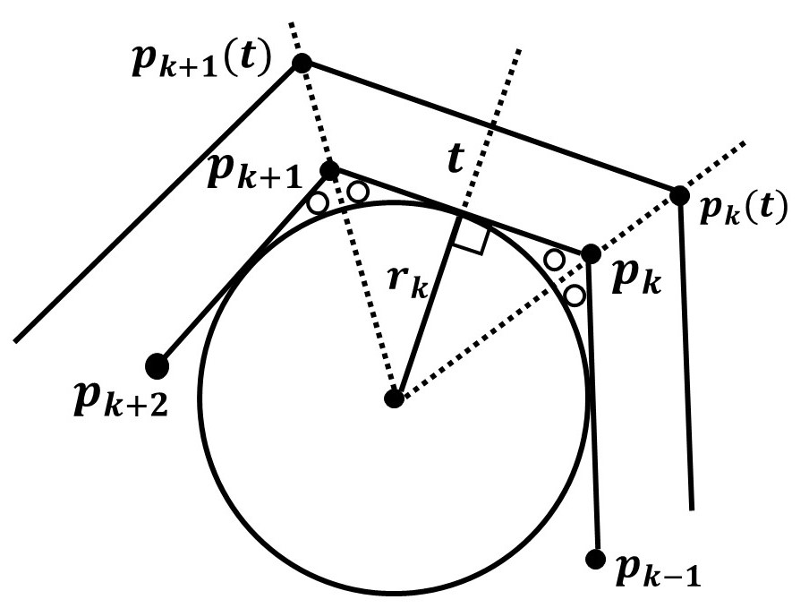
For parallel curves {pk(t)}ksubscriptsubscript𝑝𝑘𝑡𝑘\{p_{k}(t)\}_{k}, we have

|pk+1(t)pk(t)|=|pk+1pk|(1tκ(ek)),subscript𝑝𝑘1𝑡subscript𝑝𝑘𝑡subscript𝑝𝑘1subscript𝑝𝑘1𝑡𝜅subscript𝑒𝑘|p_{k+1}(t)-p_{k}(t)|=|p_{k+1}-p_{k}|(1-t\cdot\kappa(e_{k})),

where κ(ek)𝜅subscript𝑒𝑘\kappa(e_{k}) is the discrete curvature based on the edge osculating circle method [8]:

κ(ek)=tan(θk/2)+tan(θk+1/2)|pk+1pk|.𝜅subscript𝑒𝑘subscript𝜃𝑘2subscript𝜃𝑘12subscript𝑝𝑘1subscript𝑝𝑘\kappa(e_{k})=\frac{\tan(\theta_{k}/2)+\tan(\theta_{k+1}/2)}{|p_{k+1}-p_{k}|}.

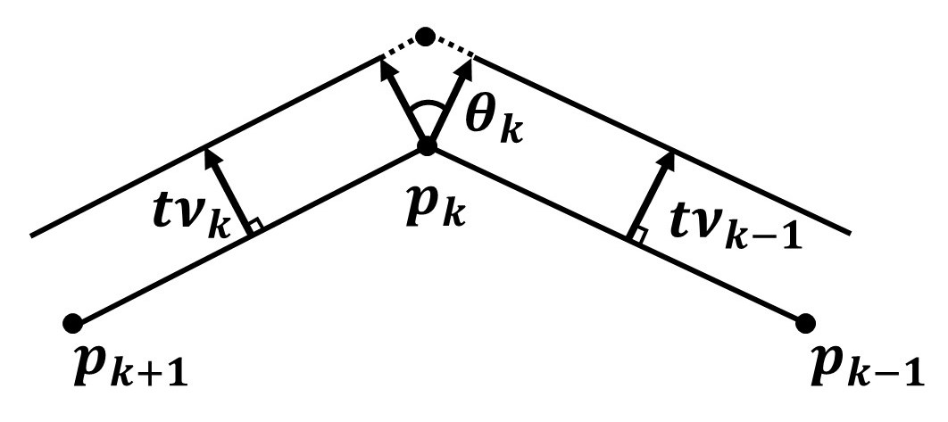
Before giving the proof, we give an intuitive explanation for a special case.
Refer to caption
Figure 2: Parallel curves

In the Figure 2, the similarity ratio of the triangles gives

|pk+1(t)pk(t)|:|pk+1pk|=(rk+t):rk|pk+1(t)pk(t)|=|pk+1pk|(1tκ(ek)).:subscript𝑝𝑘1𝑡subscript𝑝𝑘𝑡subscript𝑝𝑘1subscript𝑝𝑘subscript𝑟𝑘𝑡:subscript𝑟𝑘iffsubscript𝑝𝑘1𝑡subscript𝑝𝑘𝑡subscript𝑝𝑘1subscript𝑝𝑘1𝑡𝜅subscript𝑒𝑘\displaystyle|p_{k+1}(t)-p_{k}(t)|:|p_{k+1}-p_{k}|=(-r_{k}+t):-r_{k}\iff|p_{k+1}(t)-p_{k}(t)|=|p_{k+1}-p_{k}|(1-t\cdot\kappa(e_{k})).

Note that the signature of the curvature radius rksubscript𝑟𝑘r_{k} is negative in the figure.

Proof .

By a calculation we have

pk+1pk|pk+1pk|,Nk+1Nksubscript𝑝𝑘1subscript𝑝𝑘subscript𝑝𝑘1subscript𝑝𝑘subscript𝑁𝑘1subscript𝑁𝑘\displaystyle\left\langle\frac{p_{k+1}-p_{k}}{|p_{k+1}-p_{k}|},N_{k+1}-N_{k}\right\rangle =Rνk,νk+νk+11+cosθk+1νk1+νk1+cosθkabsent𝑅subscript𝜈𝑘subscript𝜈𝑘subscript𝜈𝑘11subscript𝜃𝑘1subscript𝜈𝑘1subscript𝜈𝑘1subscript𝜃𝑘\displaystyle=\left\langle-R\nu_{k},\frac{\nu_{k}+\nu_{k+1}}{1+\cos\theta_{k+1}}-\frac{\nu_{k-1}+\nu_{k}}{1+\cos\theta_{k}}\right\rangle
=(sinθk+11+cosθk+1+sinθk1+cosθk)=(tanθk+12+tanθk2),absentsubscript𝜃𝑘11subscript𝜃𝑘1subscript𝜃𝑘1subscript𝜃𝑘subscript𝜃𝑘12subscript𝜃𝑘2\displaystyle=-\left(\frac{\sin\theta_{k+1}}{1+\cos\theta_{k+1}}+\frac{\sin\theta_{k}}{1+\cos\theta_{k}}\right)=-\left(\tan\frac{\theta_{k+1}}{2}+\tan\frac{\theta_{k}}{2}\right),
|Nk+1Nk|2superscriptsubscript𝑁𝑘1subscript𝑁𝑘2\displaystyle|N_{k+1}-N_{k}|^{2} =1cos2(θk+1/2)+1cos2(θk/2)2Nk,Nk+1absent1superscript2subscript𝜃𝑘121superscript2subscript𝜃𝑘22subscript𝑁𝑘subscript𝑁𝑘1\displaystyle=\frac{1}{\cos^{2}(\theta_{k+1}/2)}+\frac{1}{\cos^{2}(\theta_{k}/2)}-2\langle N_{k},N_{k+1}\rangle
=2+tan2θk+12+tan2θk221+cosθk+cosθk+1+cos(θk+θk+1)(1+cosθk)(1+cosθk+1)absent2superscript2subscript𝜃𝑘12superscript2subscript𝜃𝑘221subscript𝜃𝑘subscript𝜃𝑘1subscript𝜃𝑘subscript𝜃𝑘11subscript𝜃𝑘1subscript𝜃𝑘1\displaystyle=2+\tan^{2}\frac{\theta_{k+1}}{2}+\tan^{2}\frac{\theta_{k}}{2}-2\cdot\frac{1+\cos\theta_{k}+\cos\theta_{k+1}+\cos(\theta_{k}+\theta_{k+1})}{(1+\cos\theta_{k})(1+\cos\theta_{k+1})}
=(tanθk2+tanθk+12)2.absentsuperscriptsubscript𝜃𝑘2subscript𝜃𝑘122\displaystyle=\left(\tan\frac{\theta_{k}}{2}+\tan\frac{\theta_{k+1}}{2}\right)^{2}.

Therefore we conclude

|pk+1(t)pk(t)|2superscriptsubscript𝑝𝑘1𝑡subscript𝑝𝑘𝑡2\displaystyle\qquad|p_{k+1}(t)-p_{k}(t)|^{2}
=|pk+1pk|2+2tpk+1pk,Nk+1Nk+t2|Nk+1Nk|2absentsuperscriptsubscript𝑝𝑘1subscript𝑝𝑘22𝑡subscript𝑝𝑘1subscript𝑝𝑘subscript𝑁𝑘1subscript𝑁𝑘superscript𝑡2superscriptsubscript𝑁𝑘1subscript𝑁𝑘2\displaystyle=|p_{k+1}-p_{k}|^{2}+2t\langle p_{k+1}-p_{k},N_{k+1}-N_{k}\rangle+t^{2}|N_{k+1}-N_{k}|^{2}
=|pk+1pk|22t|pk+1pk|(tanθk2+tanθk+12)+t2(tanθk2+tanθk+12)2absentsuperscriptsubscript𝑝𝑘1subscript𝑝𝑘22𝑡subscript𝑝𝑘1subscript𝑝𝑘subscript𝜃𝑘2subscript𝜃𝑘12superscript𝑡2superscriptsubscript𝜃𝑘2subscript𝜃𝑘122\displaystyle=|p_{k+1}-p_{k}|^{2}-2t|p_{k+1}-p_{k}|\left(\tan\frac{\theta_{k}}{2}+\tan\frac{\theta_{k+1}}{2}\right)+t^{2}\left(\tan\frac{\theta_{k}}{2}+\tan\frac{\theta_{k+1}}{2}\right)^{2}
=|pk+1pk|2(1ttan(θk/2)+tan(θk+1/2)|pk+1pk|)2.absentsuperscriptsubscript𝑝𝑘1subscript𝑝𝑘2superscript1𝑡subscript𝜃𝑘2subscript𝜃𝑘12subscript𝑝𝑘1subscript𝑝𝑘2\displaystyle=|p_{k+1}-p_{k}|^{2}\left(1-t\cdot\frac{\tan(\theta_{k}/2)+\tan(\theta_{k+1}/2)}{|p_{k+1}-p_{k}|}\right)^{2}.

\Box

Remark .

This formula itself is already appeared some papers to find the discrete curvature at the vertices by using the offsets, see [2], [4]. If we take the offset of the edges, then we have the following (at least) three possiblities.
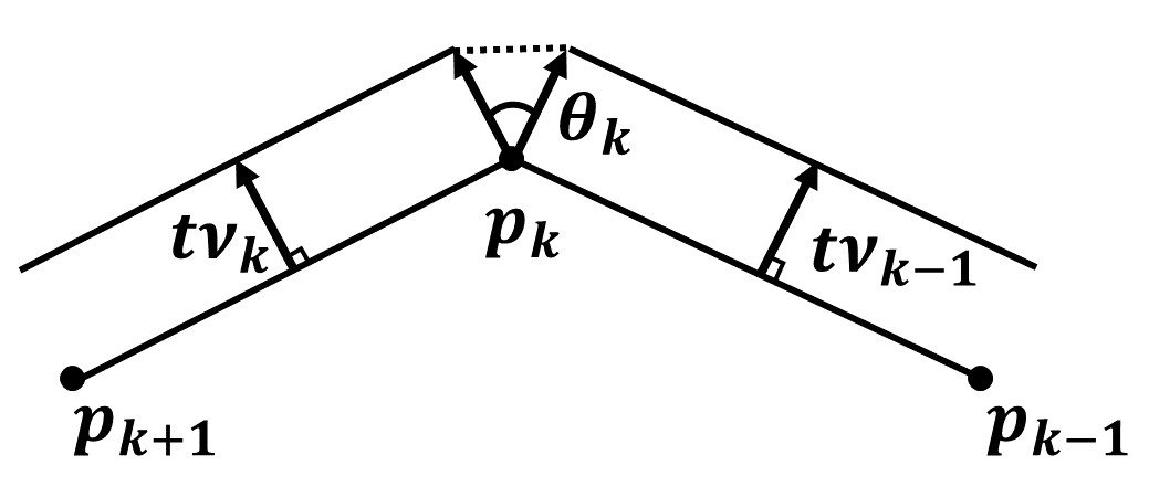
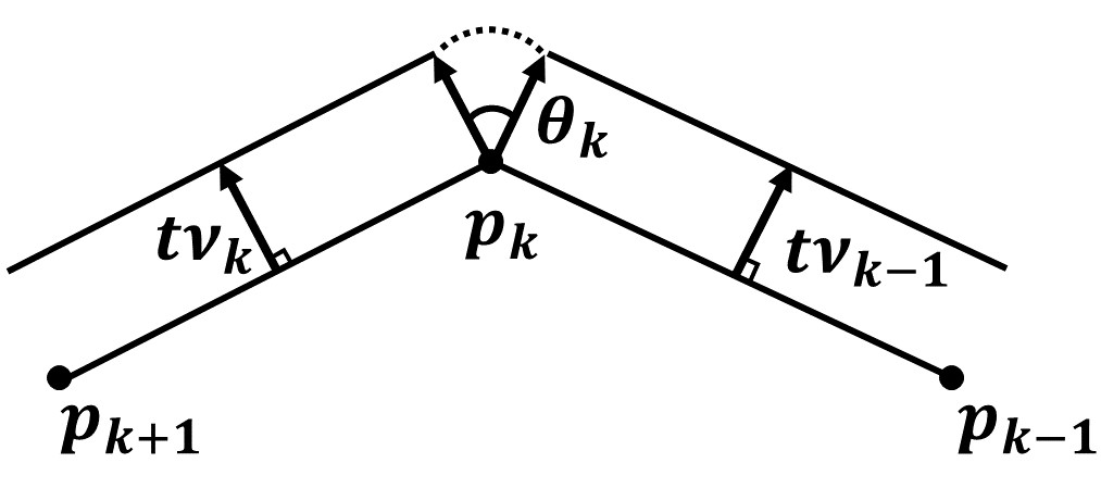
Refer to caption
(a) Γh,t(1)superscriptsubscriptΓ𝑡1\Gamma_{h,t}^{(1)}, connect by a segment
Refer to caption
(b) Γh,t(2)superscriptsubscriptΓ𝑡2\Gamma_{h,t}^{(2)}, connect by an arc
Refer to caption
(c) Γh,t(3)superscriptsubscriptΓ𝑡3\Gamma_{h,t}^{(3)}, connect by a wedge
Figure 3: Three possibilities to construct a new curve

By computing the length of dotted curves in the figure, we can write the total length of each offsets as follows:

Length(Γh,t(1))LengthsuperscriptsubscriptΓ𝑡1\displaystyle\operatorname{Length}(\Gamma_{h,t}^{(1)}) =Length(Γh)tk2sinθk2,Length(Γh,t(2))=Length(Γh)tkθk,formulae-sequenceabsentLengthsubscriptΓ𝑡subscript𝑘2subscript𝜃𝑘2LengthsuperscriptsubscriptΓ𝑡2LengthsubscriptΓ𝑡subscript𝑘subscript𝜃𝑘\displaystyle=\operatorname{Length}(\Gamma_{h})-t\sum_{k}2\sin\frac{\theta_{k}}{2},\quad\operatorname{Length}(\Gamma_{h,t}^{(2)})=\operatorname{Length}(\Gamma_{h})-t\sum_{k}\theta_{k},
Length(Γh,t(3))LengthsuperscriptsubscriptΓ𝑡3\displaystyle\operatorname{Length}(\Gamma_{h,t}^{(3)}) =Length(Γh)tk2tanθk2.absentLengthsubscriptΓ𝑡subscript𝑘2subscript𝜃𝑘2\displaystyle=\operatorname{Length}(\Gamma_{h})-t\sum_{k}2\tan\frac{\theta_{k}}{2}.

Note the signature of the angles. The second curve Γh(2)superscriptsubscriptΓ2\Gamma_{h}^{(2)} is nothing but the normal cone method (or the boundary of the Minkowski sum with the disk) known in the convex geometry. However, the only possible way to unchange the number of the vertices during the offset procedure is the third one, and by modifying the third formula gives our Steiner-type formula:

Length(Γh,t(3))LengthsuperscriptsubscriptΓ𝑡3\displaystyle\operatorname{Length}(\Gamma_{h,t}^{(3)}) =k(lk2ttan(θk/2))absentsubscript𝑘subscript𝑙𝑘2𝑡subscript𝜃𝑘2\displaystyle=\sum_{k}(l_{k}-2t\tan(\theta_{k}/2))
=k(lkt(tan(θk/2)+tan(θk+1/2)))=klk(1tκ(ek)),absentsubscript𝑘subscript𝑙𝑘𝑡subscript𝜃𝑘2subscript𝜃𝑘12subscript𝑘subscript𝑙𝑘1𝑡𝜅subscript𝑒𝑘\displaystyle=\sum_{k}(l_{k}-t(\tan(\theta_{k}/2)+\tan(\theta_{k+1}/2)))=\sum_{k}l_{k}(1-t\kappa(e_{k})),

where we put κ(ek)=(tan(θk/2)+tan(θk+1/2))/lk𝜅subscript𝑒𝑘subscript𝜃𝑘2subscript𝜃𝑘12subscript𝑙𝑘\kappa(e_{k})=(\tan(\theta_{k}/2)+\tan(\theta_{k+1}/2))/l_{k}.

Remark (Discrete Frenet-Serret formula).

In §2, we remarked that the relation

N~k= 1Lk(tktk1),tk=pk+1pk|pk+1pk|formulae-sequencesubscript~𝑁𝑘1subscript𝐿𝑘subscript𝑡𝑘subscript𝑡𝑘1subscript𝑡𝑘subscript𝑝𝑘1subscript𝑝𝑘subscript𝑝𝑘1subscript𝑝𝑘\widetilde{N}_{k}=\frac{\,1\,}{L_{k}}(t_{k}-t_{k-1}),\quad t_{k}=\frac{p_{k+1}-p_{k}}{|p_{k+1}-p_{k}|}

can be considered as a part of the Frenet-Serret formula. On the other hand, by some calculation we have

1|pk+1pk|(Nk+1Nk)=tan(θk/2)+tan(θk+1/2)|pk+1pk|tk=κ(ek)tk.1subscript𝑝𝑘1subscript𝑝𝑘subscript𝑁𝑘1subscript𝑁𝑘subscript𝜃𝑘2subscript𝜃𝑘12subscript𝑝𝑘1subscript𝑝𝑘subscript𝑡𝑘𝜅subscript𝑒𝑘subscript𝑡𝑘\frac{1}{|p_{k+1}-p_{k}|}(N_{k+1}-N_{k})=-\frac{\tan(\theta_{k}/2)+\tan(\theta_{k+1}/2)}{|p_{k+1}-p_{k}|}t_{k}=-\kappa(e_{k})t_{k}.

Note that the former formula is the formula on the vertex pksubscript𝑝𝑘p_{k} while the latter formula is the formula on the edge [pk,pk+1]subscript𝑝𝑘subscript𝑝𝑘1[p_{k},p_{k+1}].

6 The second variation formula

In this section we consider the second variation formula of the length functional. We will follow the argument developed in [11].

Let Γh={pk}ksubscriptΓsubscriptsubscript𝑝𝑘𝑘\Gamma_{h}=\{p_{k}\}_{k} be an equilibrium closed curve for the functional L+κVol𝐿𝜅VolL+\kappa\operatorname{Vol}. We say a variation is admissible (or permissible) if the variation is volume-preserving and fixes the boundary. We recall the first variation formula of the length and the 222-dimensional volume:

ddtL𝑑𝑑𝑡𝐿\displaystyle\frac{d}{dt}L =kpkL,pk,pkL=R(νkνk1),formulae-sequenceabsentsubscript𝑘subscriptsubscript𝑝𝑘𝐿superscriptsubscript𝑝𝑘subscriptsubscript𝑝𝑘𝐿𝑅subscript𝜈𝑘subscript𝜈𝑘1\displaystyle=\sum_{k}\langle\nabla_{p_{k}}L,p_{k}^{\prime}\rangle,\quad\nabla_{p_{k}}L=R(\nu_{k}-\nu_{k-1}),
ddtVol𝑑𝑑𝑡Vol\displaystyle\frac{d}{dt}\operatorname{Vol} =kpkVol,pk,pkVol=12R(pk+1pk1).formulae-sequenceabsentsubscript𝑘subscriptsubscript𝑝𝑘Volsuperscriptsubscript𝑝𝑘subscriptsubscript𝑝𝑘Vol12𝑅subscript𝑝𝑘1subscript𝑝𝑘1\displaystyle=\sum_{k}\langle\nabla_{p_{k}}\operatorname{Vol},p_{k}^{\prime}\rangle,\quad\nabla_{p_{k}}\operatorname{Vol}=\frac{1}{2}R(p_{k+1}-p_{k-1}).

Note that if the variation is admissible, then we have

0=δ2Vol=kδ(pkVol),δpk+pkVol,δ2pk.0superscript𝛿2Volsubscript𝑘𝛿subscriptsubscript𝑝𝑘Vol𝛿subscript𝑝𝑘subscriptsubscript𝑝𝑘Volsuperscript𝛿2subscript𝑝𝑘0=\delta^{2}\operatorname{Vol}=\sum_{k}\langle\delta(\nabla_{p_{k}}\operatorname{Vol}),\delta p_{k}\rangle+\langle\nabla_{p_{k}}\operatorname{Vol},\delta^{2}p_{k}\rangle.
Lemma 6.1.

Let Γh={pk}ksubscriptΓsubscriptsubscript𝑝𝑘𝑘\Gamma_{h}=\{p_{k}\}_{k} be an equilibrium closed curve for the functional L+κVol𝐿𝜅VolL+\kappa\operatorname{Vol} and pk(t)=pk+tvk+O(t2)subscript𝑝𝑘𝑡subscript𝑝𝑘𝑡subscript𝑣𝑘𝑂superscript𝑡2p_{k}(t)=p_{k}+tv_{k}+O(t^{2}) be an admissible variation. Then we have

δ2L:=d2dt2|t=0L=kδ(pkL+κpkVol),vk.\delta^{2}L:=\frac{d^{2}}{dt^{2}}_{|t=0}L=\sum_{k}\langle\delta(\nabla_{p_{k}}L+\kappa\nabla_{p_{k}}\operatorname{Vol}),v_{k}\rangle.
Definition 6.2 (Stability of discrete curves).

Let Γh={pk}ksubscriptΓsubscriptsubscript𝑝𝑘𝑘\Gamma_{h}=\{p_{k}\}_{k} be a closed equilibrium curve for the functional L+κVol𝐿𝜅VolL+\kappa\operatorname{Vol}. Then ΓhsubscriptΓ\Gamma_{h} is said to be stable if δ2L0superscript𝛿2𝐿0\delta^{2}L\geq 0 for any admissible variation.

We introduce the matrix QLsuperscript𝑄𝐿Q^{L} and QVsuperscript𝑄𝑉Q^{V} as follows:

vtQLv=kδpkL,vk,vtQVv=kδpkVol,vk.formulae-sequencesuperscript𝑣𝑡superscript𝑄𝐿𝑣subscript𝑘𝛿subscriptsubscript𝑝𝑘𝐿subscript𝑣𝑘superscript𝑣𝑡superscript𝑄𝑉𝑣subscript𝑘𝛿subscriptsubscript𝑝𝑘Volsubscript𝑣𝑘{}^{t}\vec{v}Q^{L}\vec{v}=\sum_{k}\langle\delta\nabla_{p_{k}}L,v_{k}\rangle,\quad{}^{t}\vec{v}Q^{V}\vec{v}=\sum_{k}\langle\delta\nabla_{p_{k}}\operatorname{Vol},v_{k}\rangle.

Then we can write δ2L=vt(QL+κQV)vsuperscript𝛿2𝐿superscript𝑣𝑡superscript𝑄𝐿𝜅superscript𝑄𝑉𝑣\delta^{2}L={}^{t}\vec{v}(Q^{L}+\kappa Q^{V})\vec{v}.

Lemma 6.3.

vtQVv=kvk,Rvk+1superscript𝑣𝑡superscript𝑄𝑉𝑣subscript𝑘subscript𝑣𝑘𝑅subscript𝑣𝑘1{}^{t}\vec{v}Q^{V}\vec{v}=\sum_{k}\langle v_{k},Rv_{k+1}\rangle.

Proof .

The proof follows from the direct computation:

vtQVvsuperscript𝑣𝑡superscript𝑄𝑉𝑣\displaystyle{}^{t}\vec{v}Q^{V}\vec{v} =kδpkVol,vk=12kδR(pk+1pk1),vkabsentsubscript𝑘𝛿subscriptsubscript𝑝𝑘Volsubscript𝑣𝑘12subscript𝑘𝛿𝑅subscript𝑝𝑘1subscript𝑝𝑘1subscript𝑣𝑘\displaystyle=\sum_{k}\langle\delta\nabla_{p_{k}}\operatorname{Vol},v_{k}\rangle=\frac{1}{2}\sum_{k}\langle\delta R(p_{k+1}-p_{k-1}),v_{k}\rangle
=12kR(vk+1vk1),vk=kvk,Rvk+1.absent12subscript𝑘𝑅subscript𝑣𝑘1subscript𝑣𝑘1subscript𝑣𝑘subscript𝑘subscript𝑣𝑘𝑅subscript𝑣𝑘1\displaystyle=\frac{1}{2}\sum_{k}\langle R(v_{k+1}-v_{k-1}),v_{k}\rangle=\sum_{k}\langle v_{k},Rv_{k+1}\rangle.

\Box

Proposition 6.4 (Second variation formula for the length functional).
QL=k1lk(|vk+1vk|2vk+1vk,Rνk2)=k(|vk|2vk,Rνk2)lk,superscript𝑄𝐿subscript𝑘1subscript𝑙𝑘superscriptsubscript𝑣𝑘1subscript𝑣𝑘2superscriptsubscript𝑣𝑘1subscript𝑣𝑘𝑅subscript𝜈𝑘2subscript𝑘superscriptsubscript𝑣𝑘2superscriptsubscript𝑣𝑘𝑅subscript𝜈𝑘2subscript𝑙𝑘Q^{L}=\sum_{k}\frac{1}{l_{k}}(|v_{k+1}-v_{k}|^{2}-\langle v_{k+1}-v_{k},R\nu_{k}\rangle^{2})=\sum_{k}(|\nabla v_{k}|^{2}-\langle\nabla v_{k},R\nu_{k}\rangle^{2})l_{k},

therefore we have the following second variation formula for the length functional:

δ2L=k(|vk|2vk,Rνk2)lk+κvk,Rvk+1.superscript𝛿2𝐿subscript𝑘superscriptsubscript𝑣𝑘2superscriptsubscript𝑣𝑘𝑅subscript𝜈𝑘2subscript𝑙𝑘𝜅subscript𝑣𝑘𝑅subscript𝑣𝑘1\delta^{2}L=\sum_{k}(|\nabla v_{k}|^{2}-\langle\nabla v_{k},R\nu_{k}\rangle^{2})l_{k}+\kappa\langle v_{k},Rv_{k+1}\rangle. (6.1)
Proof .

By using the fact lkδνk=R(vk+1vk)R(vk+1vk),νkνksubscript𝑙𝑘𝛿subscript𝜈𝑘𝑅subscript𝑣𝑘1subscript𝑣𝑘𝑅subscript𝑣𝑘1subscript𝑣𝑘subscript𝜈𝑘subscript𝜈𝑘l_{k}\delta\nu_{k}=R(v_{k+1}-v_{k})-\langle R(v_{k+1}-v_{k}),\nu_{k}\rangle\nu_{k}, we have

QLsuperscript𝑄𝐿\displaystyle Q^{L} =kδνk,R(vk+1vk)=kR(vk)R(vk),νkνk,R(vk)lkabsentsubscript𝑘𝛿subscript𝜈𝑘𝑅subscript𝑣𝑘1subscript𝑣𝑘subscript𝑘𝑅subscript𝑣𝑘𝑅subscript𝑣𝑘subscript𝜈𝑘subscript𝜈𝑘𝑅subscript𝑣𝑘subscript𝑙𝑘\displaystyle=\sum_{k}\langle\delta\nu_{k},R(v_{k+1}-v_{k})\rangle=\sum_{k}\langle R(\nabla v_{k})-\langle R(\nabla v_{k}),\nu_{k}\rangle\nu_{k},R(\nabla v_{k})\rangle l_{k}
=k(|vk|2R(vk),νk2)lk=k(|vk|2vk,Rνk2)lk.absentsubscript𝑘superscriptsubscript𝑣𝑘2superscript𝑅subscript𝑣𝑘subscript𝜈𝑘2subscript𝑙𝑘subscript𝑘superscriptsubscript𝑣𝑘2superscriptsubscript𝑣𝑘𝑅subscript𝜈𝑘2subscript𝑙𝑘\displaystyle=\sum_{k}(|\nabla v_{k}|^{2}-\langle R(\nabla v_{k}),\nu_{k}\rangle^{2})l_{k}=\sum_{k}(|\nabla v_{k}|^{2}-\langle\nabla v_{k},R\nu_{k}\rangle^{2})l_{k}.

\Box

In the section of the Steiner-type formula, we used the vector

Nk:=R(νk1νk)sinθk=11+cosθk(νk+νk1)assignsubscript𝑁𝑘𝑅subscript𝜈𝑘1subscript𝜈𝑘subscript𝜃𝑘11subscript𝜃𝑘subscript𝜈𝑘subscript𝜈𝑘1N_{k}:=\frac{R(\nu_{k-1}-\nu_{k})}{\sin\theta_{k}}=\frac{1}{1+\cos\theta_{k}}(\nu_{k}+\nu_{k-1})

as the “normal vector” at the vertex pksubscript𝑝𝑘p_{k}. If we define the “tangent vector” Tksubscript𝑇𝑘T_{k} as Tk=RNksubscript𝑇𝑘𝑅subscript𝑁𝑘T_{k}=-RN_{k}, then we can decompose the variation vector vksubscript𝑣𝑘v_{k} as

vk=ψkNk+ηkTk=ψkNkηkRNk,subscript𝑣𝑘subscript𝜓𝑘subscript𝑁𝑘subscript𝜂𝑘subscript𝑇𝑘subscript𝜓𝑘subscript𝑁𝑘subscript𝜂𝑘𝑅subscript𝑁𝑘v_{k}=\psi_{k}N_{k}+\eta_{k}T_{k}=\psi_{k}N_{k}-\eta_{k}RN_{k},

where ψ,η:V:𝜓𝜂𝑉\psi,\eta:V\to\mathbb{R} is some functions on the vertices. If ηk=0subscript𝜂𝑘0\eta_{k}=0 for all k𝑘k, we call the variation the normal variation. In the following we will use this notation.

Lemma 6.5.

The first variation formula of the volume can be written as

δVol=12k(ψk(lk+lk1)+ηk(lklk1)tanθk2).𝛿Vol12subscript𝑘subscript𝜓𝑘subscript𝑙𝑘subscript𝑙𝑘1subscript𝜂𝑘subscript𝑙𝑘subscript𝑙𝑘1subscript𝜃𝑘2\delta\operatorname{Vol}=\frac{1}{2}\sum_{k}\left(\psi_{k}(l_{k}+l_{k-1})+\eta_{k}(l_{k}-l_{k-1})\tan\frac{\theta_{k}}{2}\right).

In particular, if the curve Γh={pk}ksubscriptΓsubscriptsubscript𝑝𝑘𝑘\Gamma_{h}=\{p_{k}\}_{k} satisfies lkl0subscript𝑙𝑘subscript𝑙0l_{k}\equiv l_{0}, then a variation pk(t)=pk+t(ψkNk+ηkTk)+O(t2)subscript𝑝𝑘𝑡subscript𝑝𝑘𝑡subscript𝜓𝑘subscript𝑁𝑘subscript𝜂𝑘subscript𝑇𝑘𝑂superscript𝑡2p_{k}(t)=p_{k}+t(\psi_{k}N_{k}+\eta_{k}T_{k})+O(t^{2}) is volume-preserving if kψk=0subscript𝑘subscript𝜓𝑘0\sum_{k}\psi_{k}=0.

Proof .

Using the first variation formula, we have

δVol𝛿Vol\displaystyle\delta\operatorname{Vol} =12kR(pk+1pk1),vk=12kR(pk+1pk1),ψkNk+ηkTkabsent12subscript𝑘𝑅subscript𝑝𝑘1subscript𝑝𝑘1subscript𝑣𝑘12subscript𝑘𝑅subscript𝑝𝑘1subscript𝑝𝑘1subscript𝜓𝑘subscript𝑁𝑘subscript𝜂𝑘subscript𝑇𝑘\displaystyle=\frac{1}{2}\sum_{k}\langle R(p_{k+1}-p_{k-1}),v_{k}\rangle=\frac{1}{2}\sum_{k}\langle R(p_{k+1}-p_{k-1}),\psi_{k}N_{k}+\eta_{k}T_{k}\rangle
=12k[ψklkνk,Rνk1sinθk+ψklk1νk1,Rνksinθk+ηksinθk(lklk1)(1cosθk)]absent12subscript𝑘delimited-[]subscript𝜓𝑘subscript𝑙𝑘subscript𝜈𝑘𝑅subscript𝜈𝑘1subscript𝜃𝑘subscript𝜓𝑘subscript𝑙𝑘1subscript𝜈𝑘1𝑅subscript𝜈𝑘subscript𝜃𝑘subscript𝜂𝑘subscript𝜃𝑘subscript𝑙𝑘subscript𝑙𝑘11subscript𝜃𝑘\displaystyle=\frac{1}{2}\sum_{k}\left[\psi_{k}l_{k}\frac{\langle\nu_{k},R\nu_{k-1}\rangle}{\sin\theta_{k}}+\psi_{k}l_{k-1}\frac{\langle\nu_{k-1},-R\nu_{k}\rangle}{\sin\theta_{k}}+\frac{\eta_{k}}{\sin\theta_{k}}(l_{k}-l_{k-1})(1-\cos\theta_{k})\right]
=12k(ψk(lk+lk1)+ηk(lklk1)tanθk2).absent12subscript𝑘subscript𝜓𝑘subscript𝑙𝑘subscript𝑙𝑘1subscript𝜂𝑘subscript𝑙𝑘subscript𝑙𝑘1subscript𝜃𝑘2\displaystyle=\frac{1}{2}\sum_{k}\left(\psi_{k}(l_{k}+l_{k-1})+\eta_{k}(l_{k}-l_{k-1})\tan\frac{\theta_{k}}{2}\right).

\Box

Remark .

For a function ψksubscript𝜓𝑘\psi_{k} satisfying kψk=0subscript𝑘subscript𝜓𝑘0\sum_{k}\psi_{k}=0, we can find a variation whose variation vector field is ψkNksubscript𝜓𝑘subscript𝑁𝑘\psi_{k}N_{k}. The proof is completely the same as in [1].

Recall that if {pk}ksubscriptsubscript𝑝𝑘𝑘\{p_{k}\}_{k} is an equilibrium curve of the functional L+κVol𝐿𝜅VolL+\kappa\operatorname{Vol}, then we have lkl0subscript𝑙𝑘subscript𝑙0l_{k}\equiv l_{0}, θkθ0subscript𝜃𝑘subscript𝜃0\theta_{k}\equiv\theta_{0} and κl0=2tan(θ0/2)𝜅subscript𝑙02subscript𝜃02\kappa l_{0}=2\tan(\theta_{0}/2).

Lemma 6.6.
|vk+1vk|2vk+1vk,Rνk2=[(ψk+1ψk)+tan(θ0/2)(ηk+1+ηk)]2.superscriptsubscript𝑣𝑘1subscript𝑣𝑘2superscriptsubscript𝑣𝑘1subscript𝑣𝑘𝑅subscript𝜈𝑘2superscriptdelimited-[]subscript𝜓𝑘1subscript𝜓𝑘subscript𝜃02subscript𝜂𝑘1subscript𝜂𝑘2|v_{k+1}-v_{k}|^{2}-\langle v_{k+1}-v_{k},R\nu_{k}\rangle^{2}=[(\psi_{k+1}-\psi_{k})+\tan(\theta_{0}/2)(\eta_{k+1}+\eta_{k})]^{2}.

Therefore we have

|vk|2vk,Rνk2=(ψk+κ2(ηk+ηk+1))2superscriptsubscript𝑣𝑘2superscriptsubscript𝑣𝑘𝑅subscript𝜈𝑘2superscriptsubscript𝜓𝑘𝜅2subscript𝜂𝑘subscript𝜂𝑘12|\nabla v_{k}|^{2}-\langle\nabla v_{k},R\nu_{k}\rangle^{2}=\left(\nabla\psi_{k}+\frac{\kappa}{2}(\eta_{k}+\eta_{k+1})\right)^{2}
Proof .

Recall that

Nk,RNk+1subscript𝑁𝑘𝑅subscript𝑁𝑘1\displaystyle\langle N_{k},-RN_{k+1}\rangle =tanθk2+tanθk+12=2tanθ02,absentsubscript𝜃𝑘2subscript𝜃𝑘122subscript𝜃02\displaystyle=\tan\frac{\theta_{k}}{2}+\tan\frac{\theta_{k+1}}{2}=2\tan\frac{\theta_{0}}{2},
Nk,Nk+1subscript𝑁𝑘subscript𝑁𝑘1\displaystyle\langle N_{k},N_{k+1}\rangle =1tanθk2tanθk+12=1tan2θ02.absent1subscript𝜃𝑘2subscript𝜃𝑘121superscript2subscript𝜃02\displaystyle=1-\tan\frac{\theta_{k}}{2}\tan\frac{\theta_{k+1}}{2}=1-\tan^{2}\frac{\theta_{0}}{2}.

If we note |Nk|=1/cos(θ0/2)subscript𝑁𝑘1subscript𝜃02|N_{k}|=1/\cos(\theta_{0}/2), then

|vk+1vk|2superscriptsubscript𝑣𝑘1subscript𝑣𝑘2\displaystyle\qquad|v_{k+1}-v_{k}|^{2}
=|ψk+1Nk+1ψkNk|2+2ψk+1Nk+1ψkNk,ηk+1Tk+1ηkTk+|ηk+1Tk+1ηkTk|2absentsuperscriptsubscript𝜓𝑘1subscript𝑁𝑘1subscript𝜓𝑘subscript𝑁𝑘22subscript𝜓𝑘1subscript𝑁𝑘1subscript𝜓𝑘subscript𝑁𝑘subscript𝜂𝑘1subscript𝑇𝑘1subscript𝜂𝑘subscript𝑇𝑘superscriptsubscript𝜂𝑘1subscript𝑇𝑘1subscript𝜂𝑘subscript𝑇𝑘2\displaystyle=|\psi_{k+1}N_{k+1}-\psi_{k}N_{k}|^{2}+2\langle\psi_{k+1}N_{k+1}-\psi_{k}N_{k},\eta_{k+1}T_{k+1}-\eta_{k}T_{k}\rangle+|\eta_{k+1}T_{k+1}-\eta_{k}T_{k}|^{2}
=ψk+12cos2(θ0/2)2ψkψk+1(1tan2(θ0/2))+ψk2cos2(θ0/2)2Nk,RNk+1(ψk+1ηkψkηk+1)absentsuperscriptsubscript𝜓𝑘12superscript2subscript𝜃022subscript𝜓𝑘subscript𝜓𝑘11superscript2subscript𝜃02superscriptsubscript𝜓𝑘2superscript2subscript𝜃022subscript𝑁𝑘𝑅subscript𝑁𝑘1subscript𝜓𝑘1subscript𝜂𝑘subscript𝜓𝑘subscript𝜂𝑘1\displaystyle=\frac{\psi_{k+1}^{2}}{\cos^{2}(\theta_{0}/2)}-2\psi_{k}\psi_{k+1}(1-\tan^{2}(\theta_{0}/2))+\frac{\psi_{k}^{2}}{\cos^{2}(\theta_{0}/2)}-2\langle N_{k},RN_{k+1}\rangle(\psi_{k+1}\eta_{k}-\psi_{k}\eta_{k+1})
+ηk+12cos2(θ0/2)2ηkηk+1(1tan2(θ0/2))+ηk2cos2(θ0/2)superscriptsubscript𝜂𝑘12superscript2subscript𝜃022subscript𝜂𝑘subscript𝜂𝑘11superscript2subscript𝜃02superscriptsubscript𝜂𝑘2superscript2subscript𝜃02\displaystyle\qquad+\frac{\eta_{k+1}^{2}}{\cos^{2}(\theta_{0}/2)}-2\eta_{k}\eta_{k+1}(1-\tan^{2}(\theta_{0}/2))+\frac{\eta_{k}^{2}}{\cos^{2}(\theta_{0}/2)}
=(1+tan2(θ0/2))(ψk+12+ψk2+ηk+12+ηk2)absent1superscript2subscript𝜃02superscriptsubscript𝜓𝑘12superscriptsubscript𝜓𝑘2superscriptsubscript𝜂𝑘12superscriptsubscript𝜂𝑘2\displaystyle=(1+\tan^{2}(\theta_{0}/2))(\psi_{k+1}^{2}+\psi_{k}^{2}+\eta_{k+1}^{2}+\eta_{k}^{2})
2(ψkψk+1+ηkηk+1)(1tan2(θ0/2))+4tan(θ0/2)(ηkψk+1ηk+1ψk).2subscript𝜓𝑘subscript𝜓𝑘1subscript𝜂𝑘subscript𝜂𝑘11superscript2subscript𝜃024subscript𝜃02subscript𝜂𝑘subscript𝜓𝑘1subscript𝜂𝑘1subscript𝜓𝑘\displaystyle\qquad-2(\psi_{k}\psi_{k+1}+\eta_{k}\eta_{k+1})(1-\tan^{2}(\theta_{0}/2))+4\tan(\theta_{0}/2)(\eta_{k}\psi_{k+1}-\eta_{k+1}\psi_{k}).

Similarly since

vk+1vk,Rνksubscript𝑣𝑘1subscript𝑣𝑘𝑅subscript𝜈𝑘\displaystyle\qquad\langle v_{k+1}-v_{k},R\nu_{k}\rangle
=ψk+1Nk+1ψkNk+ηk+1Tk+1ηkTk,Rνkabsentsubscript𝜓𝑘1subscript𝑁𝑘1subscript𝜓𝑘subscript𝑁𝑘subscript𝜂𝑘1subscript𝑇𝑘1subscript𝜂𝑘subscript𝑇𝑘𝑅subscript𝜈𝑘\displaystyle=\langle\psi_{k+1}N_{k+1}-\psi_{k}N_{k}+\eta_{k+1}T_{k+1}-\eta_{k}T_{k},R\nu_{k}\rangle
=ψk+1νkνk+1,νksinθk+1ψkνk1νk,νksinθkηk+1νk+1νk,Rνksinθk+1+ηkνkνk1,Rνksinθkabsentsubscript𝜓𝑘1subscript𝜈𝑘subscript𝜈𝑘1subscript𝜈𝑘subscript𝜃𝑘1subscript𝜓𝑘subscript𝜈𝑘1subscript𝜈𝑘subscript𝜈𝑘subscript𝜃𝑘subscript𝜂𝑘1subscript𝜈𝑘1subscript𝜈𝑘𝑅subscript𝜈𝑘subscript𝜃𝑘1subscript𝜂𝑘subscript𝜈𝑘subscript𝜈𝑘1𝑅subscript𝜈𝑘subscript𝜃𝑘\displaystyle=\psi_{k+1}\frac{\langle\nu_{k}-\nu_{k+1},\nu_{k}\rangle}{\sin\theta_{k+1}}-\psi_{k}\frac{\langle\nu_{k-1}-\nu_{k},\nu_{k}\rangle}{\sin\theta_{k}}-\eta_{k+1}\frac{\langle\nu_{k+1}-\nu_{k},R\nu_{k}\rangle}{\sin\theta_{k+1}}+\eta_{k}\frac{\langle\nu_{k}-\nu_{k-1},R\nu_{k}\rangle}{\sin\theta_{k}}
=(ψk+1+ψk)tanθ02(ηk+1ηk),absentsubscript𝜓𝑘1subscript𝜓𝑘subscript𝜃02subscript𝜂𝑘1subscript𝜂𝑘\displaystyle=(\psi_{k+1}+\psi_{k})\tan\frac{\theta_{0}}{2}-(\eta_{k+1}-\eta_{k}),

we have

vk+1vk,Rνk2=(ψk+1+ψk)2tan2θ022tanθ02(ψk+1+ψk)(ηk+1ηk)+(ηk+1ηk)2.superscriptsubscript𝑣𝑘1subscript𝑣𝑘𝑅subscript𝜈𝑘2superscriptsubscript𝜓𝑘1subscript𝜓𝑘2superscript2subscript𝜃022subscript𝜃02subscript𝜓𝑘1subscript𝜓𝑘subscript𝜂𝑘1subscript𝜂𝑘superscriptsubscript𝜂𝑘1subscript𝜂𝑘2\langle v_{k+1}-v_{k},R\nu_{k}\rangle^{2}=(\psi_{k+1}+\psi_{k})^{2}\tan^{2}\frac{\theta_{0}}{2}-2\tan\frac{\theta_{0}}{2}(\psi_{k+1}+\psi_{k})(\eta_{k+1}-\eta_{k})+(\eta_{k+1}-\eta_{k})^{2}.

Substracting these factors we have

|vk+1vk|2vk+1vk,Rνk2superscriptsubscript𝑣𝑘1subscript𝑣𝑘2superscriptsubscript𝑣𝑘1subscript𝑣𝑘𝑅subscript𝜈𝑘2\displaystyle\qquad|v_{k+1}-v_{k}|^{2}-\langle v_{k+1}-v_{k},R\nu_{k}\rangle^{2}
=ψk+12+ψk2+tan2θ02(ηk+12+ηk2)2ψkψk+1tan2θ02+2ηkηk+1absentsuperscriptsubscript𝜓𝑘12superscriptsubscript𝜓𝑘2superscript2subscript𝜃02superscriptsubscript𝜂𝑘12superscriptsubscript𝜂𝑘22subscript𝜓𝑘subscript𝜓𝑘1superscript2subscript𝜃022subscript𝜂𝑘subscript𝜂𝑘1\displaystyle=\psi_{k+1}^{2}+\psi_{k}^{2}+\tan^{2}\frac{\theta_{0}}{2}(\eta_{k+1}^{2}+\eta_{k}^{2})-2\psi_{k}\psi_{k+1}\tan^{2}\frac{\theta_{0}}{2}+2\eta_{k}\eta_{k+1}
+2tanθ02(2ηkψk+12ηk+1ψk+ψk+1ηk+1ψk+1ηk+ψkηk+1ψkηk)2subscript𝜃022subscript𝜂𝑘subscript𝜓𝑘12subscript𝜂𝑘1subscript𝜓𝑘subscript𝜓𝑘1subscript𝜂𝑘1subscript𝜓𝑘1subscript𝜂𝑘subscript𝜓𝑘subscript𝜂𝑘1subscript𝜓𝑘subscript𝜂𝑘\displaystyle\qquad+2\tan\frac{\theta_{0}}{2}(2\eta_{k}\psi_{k+1}-2\eta_{k+1}\psi_{k}+\psi_{k+1}\eta_{k+1}-\psi_{k+1}\eta_{k}+\psi_{k}\eta_{k+1}-\psi_{k}\eta_{k})
2(ψkψk+1+ηkηk+1)+2tan2θ02(ψkψk+1+ηkηk+1)2subscript𝜓𝑘subscript𝜓𝑘1subscript𝜂𝑘subscript𝜂𝑘12superscript2subscript𝜃02subscript𝜓𝑘subscript𝜓𝑘1subscript𝜂𝑘subscript𝜂𝑘1\displaystyle\qquad\qquad-2(\psi_{k}\psi_{k+1}+\eta_{k}\eta_{k+1})+2\tan^{2}\frac{\theta_{0}}{2}(\psi_{k}\psi_{k+1}+\eta_{k}\eta_{k+1})
=(ψk+1ψk)2+tan2θ02(ηk+1+ηk)2+2tanθ02(ψk+1ψk)(ηk+1+ηk)absentsuperscriptsubscript𝜓𝑘1subscript𝜓𝑘2superscript2subscript𝜃02superscriptsubscript𝜂𝑘1subscript𝜂𝑘22subscript𝜃02subscript𝜓𝑘1subscript𝜓𝑘subscript𝜂𝑘1subscript𝜂𝑘\displaystyle=(\psi_{k+1}-\psi_{k})^{2}+\tan^{2}\frac{\theta_{0}}{2}(\eta_{k+1}+\eta_{k})^{2}+2\tan\frac{\theta_{0}}{2}(\psi_{k+1}-\psi_{k})(\eta_{k+1}+\eta_{k})
=[(ψk+1ψk)+tanθ02(ηk+1+ηk)]2absentsuperscriptdelimited-[]subscript𝜓𝑘1subscript𝜓𝑘subscript𝜃02subscript𝜂𝑘1subscript𝜂𝑘2\displaystyle=[(\psi_{k+1}-\psi_{k})+\tan\frac{\theta_{0}}{2}(\eta_{k+1}+\eta_{k})]^{2}

\Box

Lemma 6.7.
vk,Rvk+1=2tanθ02(ψkψk+1+ηkηk+1)(1tan2θ22)(ηkψk+1ηk+1ψk).subscript𝑣𝑘𝑅subscript𝑣𝑘12subscript𝜃02subscript𝜓𝑘subscript𝜓𝑘1subscript𝜂𝑘subscript𝜂𝑘11superscript2subscript𝜃22subscript𝜂𝑘subscript𝜓𝑘1subscript𝜂𝑘1subscript𝜓𝑘\langle v_{k},Rv_{k+1}\rangle=-2\tan\frac{\theta_{0}}{2}(\psi_{k}\psi_{k+1}+\eta_{k}\eta_{k+1})-(1-\tan^{2}\frac{\theta_{2}}{2})(\eta_{k}\psi_{k+1}-\eta_{k+1}\psi_{k}).
Proof .

This is also a simple calculation:

vk,Rvk+1subscript𝑣𝑘𝑅subscript𝑣𝑘1\displaystyle\langle v_{k},Rv_{k+1}\rangle =ψkNkηkRNk,ψk+1RNk+1+ηk+1Nk+1absentsubscript𝜓𝑘subscript𝑁𝑘subscript𝜂𝑘𝑅subscript𝑁𝑘subscript𝜓𝑘1𝑅subscript𝑁𝑘1subscript𝜂𝑘1subscript𝑁𝑘1\displaystyle=\langle\psi_{k}N_{k}-\eta_{k}RN_{k},\psi_{k+1}RN_{k+1}+\eta_{k+1}N_{k+1}\rangle
=(ψkψk+1+ηkηk+1)Nk,RNk+1(ηkψk+1ηk+1ψk)Nk,Nk+1absentsubscript𝜓𝑘subscript𝜓𝑘1subscript𝜂𝑘subscript𝜂𝑘1subscript𝑁𝑘𝑅subscript𝑁𝑘1subscript𝜂𝑘subscript𝜓𝑘1subscript𝜂𝑘1subscript𝜓𝑘subscript𝑁𝑘subscript𝑁𝑘1\displaystyle=(\psi_{k}\psi_{k+1}+\eta_{k}\eta_{k+1})\langle N_{k},RN_{k+1}\rangle-(\eta_{k}\psi_{k+1}-\eta_{k+1}\psi_{k})\langle N_{k},N_{k+1}\rangle
=2tanθ02(ψkψk+1+ηkηk+1)(1tan2θ02)(ηkψk+1ηk+1ψk).absent2subscript𝜃02subscript𝜓𝑘subscript𝜓𝑘1subscript𝜂𝑘subscript𝜂𝑘11superscript2subscript𝜃02subscript𝜂𝑘subscript𝜓𝑘1subscript𝜂𝑘1subscript𝜓𝑘\displaystyle=-2\tan\frac{\theta_{0}}{2}(\psi_{k}\psi_{k+1}+\eta_{k}\eta_{k+1})-(1-\tan^{2}\frac{\theta_{0}}{2})(\eta_{k}\psi_{k+1}-\eta_{k+1}\psi_{k}).

\Box

Theorem 6.8 (Second variation formula for the length functional).
δ2L=k[|ψk|2κ2ψkψk+1+tan2θ02(κψk(ηk+1+ηk)+|ηk|2)]l0superscript𝛿2𝐿subscript𝑘delimited-[]superscriptsubscript𝜓𝑘2superscript𝜅2subscript𝜓𝑘subscript𝜓𝑘1superscript2subscript𝜃02𝜅subscript𝜓𝑘subscript𝜂𝑘1subscript𝜂𝑘superscriptsubscript𝜂𝑘2subscript𝑙0\displaystyle\delta^{2}L=\sum_{k}\left[|\nabla\psi_{k}|^{2}-\kappa^{2}\psi_{k}\psi_{k+1}+\tan^{2}\frac{\theta_{0}}{2}(\kappa\nabla\psi_{k}(\eta_{k+1}+\eta_{k})+|\nabla\eta_{k}|^{2})\right]l_{0}

In particular, for the normal variation we have

δ2L=k(|ψk|2κ2ψkψk+1)l0=kψk(Δψk+κ2ψk+1)l0,superscript𝛿2𝐿subscript𝑘superscriptsubscript𝜓𝑘2superscript𝜅2subscript𝜓𝑘subscript𝜓𝑘1subscript𝑙0subscript𝑘subscript𝜓𝑘Δsubscript𝜓𝑘superscript𝜅2subscript𝜓𝑘1subscript𝑙0\delta^{2}L=\sum_{k}(|\nabla\psi_{k}|^{2}-\kappa^{2}\psi_{k}\psi_{k+1})l_{0}=-\sum_{k}\psi_{k}(\Delta\psi_{k}+\kappa^{2}\psi_{k+1})l_{0},

where we use the integration by parts and take the line element at the vertex as Lk=(lk+lk1)/2=l0subscript𝐿𝑘subscript𝑙𝑘subscript𝑙𝑘12subscript𝑙0L_{k}=(l_{k}+l_{k-1})/2=l_{0}.

Proof .

By using the previous lemmas, we have

(|vk|2vk,Rνk2)lk+κvk,Rvk+1superscriptsubscript𝑣𝑘2superscriptsubscript𝑣𝑘𝑅subscript𝜈𝑘2subscript𝑙𝑘𝜅subscript𝑣𝑘𝑅subscript𝑣𝑘1\displaystyle\qquad(|\nabla v_{k}|^{2}-\langle\nabla v_{k},R\nu_{k}\rangle^{2})l_{k}+\kappa\langle v_{k},Rv_{k+1}\rangle
=(|ψk|2+κψk(ηk+1+ηk)+κ24(ηk+1+ηk)2)l0absentsuperscriptsubscript𝜓𝑘2𝜅subscript𝜓𝑘subscript𝜂𝑘1subscript𝜂𝑘superscript𝜅24superscriptsubscript𝜂𝑘1subscript𝜂𝑘2subscript𝑙0\displaystyle=\left(|\nabla\psi_{k}|^{2}+\kappa\nabla\psi_{k}(\eta_{k+1}+\eta_{k})+\frac{\kappa^{2}}{4}(\eta_{k+1}+\eta_{k})^{2}\right)l_{0}
κ2l0(ψkψk+1+ηkηk+1)κ(1tan2θ02)(ηkψk+1ηk+1ψk)superscript𝜅2subscript𝑙0subscript𝜓𝑘subscript𝜓𝑘1subscript𝜂𝑘subscript𝜂𝑘1𝜅1superscript2subscript𝜃02subscript𝜂𝑘subscript𝜓𝑘1subscript𝜂𝑘1subscript𝜓𝑘\displaystyle\qquad-\kappa^{2}l_{0}(\psi_{k}\psi_{k+1}+\eta_{k}\eta_{k+1})-\kappa(1-\tan^{2}\frac{\theta_{0}}{2})(\eta_{k}\psi_{k+1}-\eta_{k+1}\psi_{k})
=|ψk|2l0+κψk(ηk+1+ηk)l0+κ24(ηk+1ηk)2l0κ2ψkψk+1l0absentsuperscriptsubscript𝜓𝑘2subscript𝑙0𝜅subscript𝜓𝑘subscript𝜂𝑘1subscript𝜂𝑘subscript𝑙0superscript𝜅24superscriptsubscript𝜂𝑘1subscript𝜂𝑘2subscript𝑙0superscript𝜅2subscript𝜓𝑘subscript𝜓𝑘1subscript𝑙0\displaystyle=|\nabla\psi_{k}|^{2}l_{0}+\kappa\nabla\psi_{k}(\eta_{k+1}+\eta_{k})l_{0}+\frac{\kappa^{2}}{4}(\eta_{k+1}-\eta_{k})^{2}l_{0}-\kappa^{2}\psi_{k}\psi_{k+1}l_{0}
κ(1tan2θ22)((ψk+1ψk)(ηk+1+ηk)(ψk+1ηk+1ψkηk))𝜅1superscript2subscript𝜃22subscript𝜓𝑘1subscript𝜓𝑘subscript𝜂𝑘1subscript𝜂𝑘subscript𝜓𝑘1subscript𝜂𝑘1subscript𝜓𝑘subscript𝜂𝑘\displaystyle\qquad-\kappa(1-\tan^{2}\frac{\theta_{2}}{2})((\psi_{k+1}-\psi_{k})(\eta_{k+1}+\eta_{k})-(\psi_{k+1}\eta_{k+1}-\psi_{k}\eta_{k}))
=|ψk|2l0+κtan2θ02ψk(ηk+1+ηk)l0+κ24(ηk+1ηk)2l0κ2ψkψk+1l0absentsuperscriptsubscript𝜓𝑘2subscript𝑙0𝜅superscript2subscript𝜃02subscript𝜓𝑘subscript𝜂𝑘1subscript𝜂𝑘subscript𝑙0superscript𝜅24superscriptsubscript𝜂𝑘1subscript𝜂𝑘2subscript𝑙0superscript𝜅2subscript𝜓𝑘subscript𝜓𝑘1subscript𝑙0\displaystyle=|\nabla\psi_{k}|^{2}l_{0}+\kappa\tan^{2}\frac{\theta_{0}}{2}\nabla\psi_{k}(\eta_{k+1}+\eta_{k})l_{0}+\frac{\kappa^{2}}{4}(\eta_{k+1}-\eta_{k})^{2}l_{0}-\kappa^{2}\psi_{k}\psi_{k+1}l_{0}
+κ(1tan2θ02)(ψk+1ηk+1ψkηk).𝜅1superscript2subscript𝜃02subscript𝜓𝑘1subscript𝜂𝑘1subscript𝜓𝑘subscript𝜂𝑘\displaystyle\qquad+\kappa(1-\tan^{2}\frac{\theta_{0}}{2})(\psi_{k+1}\eta_{k+1}-\psi_{k}\eta_{k}).

Taking the summation, we have the desired result. \Box

7 Instability of non-convex regular polygons

In this section we will prove that non-convex regular polygons and convex regular polygons with multiplicity are unstable. To prove this, we find a special variation with a help of the following discrete version of Wirtinger’s inequality:

Theorem 7.1 (Discrete Wirtinger’s inequality, [6]).

Let ψ0,,ψnsubscript𝜓0subscript𝜓𝑛\psi_{0},\ldots,\psi_{n} be (n+1)𝑛1(n+1) real numbers such that

ψ0=ψn,k=0n1ψk=0.formulae-sequencesubscript𝜓0subscript𝜓𝑛superscriptsubscript𝑘0𝑛1subscript𝜓𝑘0\psi_{0}=\psi_{n},\quad\sum_{k=0}^{n-1}\psi_{k}=0.

Then we have

k=0n1(ψk+1ψk)24sin2πnk=0n1ψk2superscriptsubscript𝑘0𝑛1superscriptsubscript𝜓𝑘1subscript𝜓𝑘24superscript2𝜋𝑛superscriptsubscript𝑘0𝑛1superscriptsubscript𝜓𝑘2\sum_{k=0}^{n-1}(\psi_{k+1}-\psi_{k})^{2}\geq 4\sin^{2}\frac{\,\pi\,}{n}\sum_{k=0}^{n-1}\psi_{k}^{2} (7.1)

and the equality holds if and only if there exist A,B𝐴𝐵A,B\in\mathbb{R} such that

ψk=Acos 2πkn+Bsin 2πkn.subscript𝜓𝑘𝐴2𝜋𝑘𝑛𝐵2𝜋𝑘𝑛\psi_{k}=A\cos\frac{\,2\pi k\,}{n}+B\sin\frac{\,2\pi k\,}{n}.

In the following, we will consider the normal variation, i.e., the variation which have the form:

pk(t)=pk+tψkNk+O(t2),Nk=(νk+νk1)/(1+cosθ0),formulae-sequencesubscript𝑝𝑘𝑡subscript𝑝𝑘𝑡subscript𝜓𝑘subscript𝑁𝑘𝑂superscript𝑡2subscript𝑁𝑘subscript𝜈𝑘subscript𝜈𝑘11subscript𝜃0p_{k}(t)=p_{k}+t\psi_{k}N_{k}+O(t^{2}),\quad N_{k}=(\nu_{k}+\nu_{k-1})/(1+\cos\theta_{0}),

where ψksubscript𝜓𝑘\psi_{k} satisfies kψk=0subscript𝑘subscript𝜓𝑘0\sum_{k}\psi_{k}=0. By the second variation formula (Theorem 6.8) we have

δ2L=k(|ψk|2κ2ψkψk+1)l0=k 1l0[(ψk+1ψk)24ψkψk+1tan2mπn]superscript𝛿2𝐿subscript𝑘superscriptsubscript𝜓𝑘2superscript𝜅2subscript𝜓𝑘subscript𝜓𝑘1subscript𝑙0subscript𝑘1subscript𝑙0delimited-[]superscriptsubscript𝜓𝑘1subscript𝜓𝑘24subscript𝜓𝑘subscript𝜓𝑘1superscript2𝑚𝜋𝑛\delta^{2}L=\sum_{k}(|\nabla\psi_{k}|^{2}-\kappa^{2}\psi_{k}\psi_{k+1})l_{0}=\sum_{k}\frac{\,1\,}{l_{0}}\left[(\psi_{k+1}-\psi_{k})^{2}-4\psi_{k}\psi_{k+1}\tan^{2}\frac{\,m\pi\,}{n}\right]

for any admissible variations, where we use the relation κl0=2tan(θ0/2)𝜅subscript𝑙02subscript𝜃02\kappa l_{0}=2\tan(\theta_{0}/2) and put θ0=2mπ/nsubscript𝜃02𝑚𝜋𝑛\theta_{0}=2m\pi/n for some m𝑚m\in\mathbb{Z} and assume that m/n1/2𝑚𝑛12m/n\neq 1/2.

Theorem 7.2 (Instability of non-convex regular polygons).

Let n5𝑛5n\geq 5. By taking ψk=Acos(2πk/n)+Bsin(2πk/n)subscript𝜓𝑘𝐴2𝜋𝑘𝑛𝐵2𝜋𝑘𝑛\psi_{k}=A\cos(2\pi k/n)+B\sin(2\pi k/n), (A,B)(0,0)𝐴𝐵00(A,B)\neq(0,0), we have

δ2Length= 4l0[sin2πncos 2πntan2mπn]kψk2.superscript𝛿2Length4subscript𝑙0delimited-[]superscript2𝜋𝑛2𝜋𝑛superscript2𝑚𝜋𝑛subscript𝑘superscriptsubscript𝜓𝑘2\delta^{2}\operatorname{Length}=\frac{\,4\,}{l_{0}}\left[\sin^{2}\frac{\,\pi\,}{n}-\cos\frac{\,2\pi\,}{n}\tan^{2}\frac{\,m\pi\,}{n}\right]\sum_{k}\psi_{k}^{2}.

In particular, δ2Length<0superscript𝛿2Length0\delta^{2}\operatorname{Length}<0 for 2mn22𝑚𝑛22\leq m\leq n-2, i.e., non-convex regular polygons are unstable.

Proof.

By the discrete Wirtinger’s inequality we have

δ2Lengthk 4l0(ψk2sin2πnψkψk+1tan2mπn).superscript𝛿2Lengthsubscript𝑘4subscript𝑙0superscriptsubscript𝜓𝑘2superscript2𝜋𝑛subscript𝜓𝑘subscript𝜓𝑘1superscript2𝑚𝜋𝑛\delta^{2}\operatorname{Length}\geq\sum_{k}\frac{\,4\,}{l_{0}}(\psi_{k}^{2}\sin^{2}\frac{\pi}{n}-\psi_{k}\psi_{k+1}\tan^{2}\frac{m\pi}{n}).

In the following we use the equality condition ψk=Acos(2πk/n)+Bsin(2πk/n)subscript𝜓𝑘𝐴2𝜋𝑘𝑛𝐵2𝜋𝑘𝑛\psi_{k}=A\cos(2\pi k/n)+B\sin(2\pi k/n) and put φk=Asin(2πk/n)+Bcos(2πk/n)subscript𝜑𝑘𝐴2𝜋𝑘𝑛𝐵2𝜋𝑘𝑛\varphi_{k}=-A\sin(2\pi k/n)+B\cos(2\pi k/n). Then we have

ψk+1=ψkcos(2π/n)+φksin(2π/n),ψkφk= 12(B2A2)sin4kπn+ABcos4kπn.formulae-sequencesubscript𝜓𝑘1subscript𝜓𝑘2𝜋𝑛subscript𝜑𝑘2𝜋𝑛subscript𝜓𝑘subscript𝜑𝑘12superscript𝐵2superscript𝐴24𝑘𝜋𝑛𝐴𝐵4𝑘𝜋𝑛\psi_{k+1}=\psi_{k}\cos(2\pi/n)+\varphi_{k}\sin(2\pi/n),\quad\psi_{k}\varphi_{k}=\frac{\,1\,}{2}(B^{2}-A^{2})\sin\frac{4k\pi}{n}+AB\cos\frac{4k\pi}{n}.

If we note the fact kψkφk=0subscript𝑘subscript𝜓𝑘subscript𝜑𝑘0\sum_{k}\psi_{k}\varphi_{k}=0, then

δ2Lengthsuperscript𝛿2Length\displaystyle\delta^{2}\operatorname{Length} =k 4l0[ψk2sin2πnψk(ψkcos2πn+φksin2πn)tan2mπn]absentsubscript𝑘4subscript𝑙0delimited-[]superscriptsubscript𝜓𝑘2superscript2𝜋𝑛subscript𝜓𝑘subscript𝜓𝑘2𝜋𝑛subscript𝜑𝑘2𝜋𝑛superscript2𝑚𝜋𝑛\displaystyle=\sum_{k}\frac{\,4\,}{l_{0}}\left[\psi_{k}^{2}\sin^{2}\frac{\,\pi\,}{n}-\psi_{k}\left(\psi_{k}\cos\frac{2\pi}{n}+\varphi_{k}\sin\frac{2\pi}{n}\right)\tan^{2}\frac{m\pi}{n}\right]
= 4l0[sin2πncos2πntan2mπn]kψk2.absent4subscript𝑙0delimited-[]superscript2𝜋𝑛2𝜋𝑛superscript2𝑚𝜋𝑛subscript𝑘superscriptsubscript𝜓𝑘2\displaystyle=\frac{\,4\,}{l_{0}}\left[\sin^{2}\frac{\,\pi\,}{n}-\cos\frac{2\pi}{n}\tan^{2}\frac{m\pi}{n}\right]\sum_{k}\psi_{k}^{2}.

If m=1𝑚1m=1 or m=n1𝑚𝑛1m=n-1, then

δ2Length 4l0sin2πntan2πnkψk20.superscript𝛿2Length4subscript𝑙0superscript2𝜋𝑛superscript2𝜋𝑛subscript𝑘superscriptsubscript𝜓𝑘20\delta^{2}\operatorname{Length}\geq\frac{\,4\,}{l_{0}}\sin^{2}\frac{\,\pi\,}{n}\tan^{2}\frac{\,\pi\,}{n}\sum_{k}\psi_{k}^{2}\geq 0.

On the other hand, for 2mn22𝑚𝑛22\leq m\leq n-2 and (A,B)(0,0)𝐴𝐵00(A,B)\neq(0,0) we have

δ2Length 4sin2(π/n)(1+2cos2(π/n))l0cos(2π/n)kψk2<0,superscript𝛿2Length4superscript2𝜋𝑛12superscript2𝜋𝑛subscript𝑙02𝜋𝑛subscript𝑘superscriptsubscript𝜓𝑘20\delta^{2}\operatorname{Length}\leq-\frac{\,4\sin^{2}(\pi/n)(1+2\cos^{2}(\pi/n))\,}{l_{0}\cos(2\pi/n)}\sum_{k}\psi_{k}^{2}<0,

where we use the fact tan2(mπ/n)tan2(2π/n)superscript2𝑚𝜋𝑛superscript22𝜋𝑛\tan^{2}(m\pi/n)\geq\tan^{2}(2\pi/n) if 2mn22𝑚𝑛22\leq m\leq n-2, and cos(2π/n)>02𝜋𝑛0\cos(2\pi/n)>0 if n5𝑛5n\geq 5. This proves the statement. \Box

8 Appendix

We observe the second variation formula from the analysis of the Jacobi operator. We can modify the equation (7.1) as follows:

δ2L= 1l0k(αψk1+2ψkαψk+1)ψk= 1l0HΨ,Ψ,superscript𝛿2𝐿1subscript𝑙0subscript𝑘𝛼subscript𝜓𝑘12subscript𝜓𝑘𝛼subscript𝜓𝑘1subscript𝜓𝑘1subscript𝑙0𝐻ΨΨ\displaystyle\delta^{2}L=\frac{\,1\,}{l_{0}}\sum_{k}(-\alpha\psi_{k-1}+2\psi_{k}-\alpha\psi_{k+1})\psi_{k}=\frac{\,1\,}{l_{0}}\langle H\Psi,\Psi\rangle,

where we put α=1+2tan2(mπ/n)𝛼12superscript2𝑚𝜋𝑛\alpha=1+2\tan^{2}(m\pi/n) and

H=(2α00αα2α000α2000002αα00α2),Ψ=(ψ1ψ2ψ3ψn).formulae-sequence𝐻matrix2𝛼00𝛼𝛼2𝛼000𝛼2000002𝛼𝛼00𝛼2Ψmatrixsubscript𝜓1subscript𝜓2subscript𝜓3subscript𝜓𝑛H=\begin{pmatrix}2&-\alpha&0&\cdots&0&-\alpha\\ -\alpha&2&-\alpha&\cdots&0&0\\ 0&-\alpha&2&\cdots&0&0\\ \vdots&\vdots&\vdots&\ddots&\vdots&\vdots\\ 0&0&0&\cdots&2&-\alpha\\ -\alpha&0&0&\cdots&-\alpha&2\\ \end{pmatrix},\quad\Psi=\begin{pmatrix}\psi_{1}\\ \psi_{2}\\ \psi_{3}\\ \vdots\\ \psi_{n}\end{pmatrix}.

Since the matrix H𝐻H is the circulant matrix, the eigenvalues λjsubscript𝜆𝑗\lambda_{j} can be calculated explicitly, see e.g. [5]:

λj=22αcos2πjn=4cos2(jπ/n)cos2(mπ/n)(tan2jπnsin2mπn),j=1,,n.formulae-sequencesubscript𝜆𝑗22𝛼2𝜋𝑗𝑛4superscript2𝑗𝜋𝑛superscript2𝑚𝜋𝑛superscript2𝑗𝜋𝑛superscript2𝑚𝜋𝑛𝑗1𝑛\lambda_{j}=2-2\alpha\cos\frac{2\pi j}{n}=\frac{4\cos^{2}(j\pi/n)}{\cos^{2}(m\pi/n)}\left(\tan^{2}\frac{j\pi}{n}-\sin^{2}\frac{m\pi}{n}\right),\quad j=1,\ldots,n.

The corresponding eigenvectors are

ej=(1,ωj,,ωj(n1))tn,ω=exp(2π1/n).e_{j}={}^{t}(1,\omega^{j},\ldots,\omega^{j(n-1)})\in\mathbb{C}^{n},\quad\omega=\exp(2\pi\sqrt{-1}/n). (8.1)

The condition kψk=0subscript𝑘subscript𝜓𝑘0\sum_{k}\psi_{k}=0 is equivalent to the condition that Ψ=(ψ1,,ψn)t\Psi={}^{t}(\psi_{1},\ldots,\psi_{n}) is perpendicular to en=(1,,1)te_{n}={}^{t}(1,\ldots,1). Therefore we only consider the eigenvalues λ1,,λn1subscript𝜆1subscript𝜆𝑛1\lambda_{1},\ldots,\lambda_{n-1}.

Lemma 8.1.

For mjnm𝑚𝑗𝑛𝑚m\leq j\leq n-m, we have λj>0subscript𝜆𝑗0\lambda_{j}>0. In particular, λj>0subscript𝜆𝑗0\lambda_{j}>0 for 1jn11𝑗𝑛11\leq j\leq n-1 if m=1𝑚1m=1, i.e., the convex regular polygon case.

Proof .

This is a direct calculation:

tan2jπnsin2mπntan2mπnsin2mπn=sin2mπntan2mπn>0.superscript2𝑗𝜋𝑛superscript2𝑚𝜋𝑛superscript2𝑚𝜋𝑛superscript2𝑚𝜋𝑛superscript2𝑚𝜋𝑛superscript2𝑚𝜋𝑛0\tan^{2}\frac{j\pi}{n}-\sin^{2}\frac{m\pi}{n}\geq\tan^{2}\frac{m\pi}{n}-\sin^{2}\frac{m\pi}{n}=\sin^{2}\frac{m\pi}{n}\tan^{2}\frac{m\pi}{n}>0.
Theorem 8.2.

Assume m2𝑚2m\geq 2. For 1jm/21𝑗𝑚21\leq j\leq m/2 or nm/2jn1𝑛𝑚2𝑗𝑛1n-m/2\leq j\leq n-1, we have λj<0subscript𝜆𝑗0\lambda_{j}<0. Therefore, the index of a non-convex regular polygon or a convex polygon with multiplicity is at least m/2𝑚2\lfloor m/2\rfloor.

Proof .

Under the above conditions, we have

tan2jπnsin2mπntan2jπnsin22jπn<0.superscript2𝑗𝜋𝑛superscript2𝑚𝜋𝑛superscript2𝑗𝜋𝑛superscript22𝑗𝜋𝑛0\tan^{2}\frac{j\pi}{n}-\sin^{2}\frac{m\pi}{n}\leq\tan^{2}\frac{j\pi}{n}-\sin^{2}\frac{2j\pi}{n}<0.

\Box

Remark .

More precisely, λj<0subscript𝜆𝑗0\lambda_{j}<0 for j<(n/π)arctan(sin(mπ/n))𝑗𝑛𝜋𝑚𝜋𝑛j<(n/\pi)\arctan(\sin(m\pi/n)).

Remark .

From another point of view, a non-convex regular polygon is the high-frequency component of the discrete Fourier expansion of the polygon. More precisely, any polygon in 2superscript2\mathbb{R}^{2} with n𝑛n-vertices can be regarded as a point in 2nnsimilar-to-or-equalssuperscript2𝑛superscript𝑛\mathbb{R}^{2n}\simeq\mathbb{C}^{n}. Each eigenvector eksubscript𝑒𝑘e_{k} in (8.1) corresponds to the regular n𝑛n-gon and {e1,,en}subscript𝑒1subscript𝑒𝑛\{e_{1},\ldots,e_{n}\} forms a basis of nsuperscript𝑛\mathbb{C}^{n}. Therefore, any polygon in 2superscript2\mathbb{R}^{2} can be written as a linear combination of the regular n𝑛n-gons and this fact corresponds to the discrete Fourier expansion.

Acknowledgements

The author would like to experess his gratitude to Professor Miyuki Koiso and Professor Hisashi Naito for invaluable comments and friutful discussions.

References

  • [1] Barbosa, J. L. and do Carmo, M.: Stability of hypersurfaces with constant mean curvature, Math. Z. 185 (1984), 339–353.
  • [2] Bauer, U., Polthier, K., and Wardetzky, M.: Uniform convergence of discrete curvatures from nets of curvature lines, Discrete comput. geom. 43 (2010), 798–823.
  • [3] Chow B., and Glickenstein, D.: Semidiscrete Geometric Flow of Polygon, Amer. Math. Monthly 114, No. 4 (2007), 316–328.
  • [4] Crane, K., and Wardetzky, M.: A Glimpse into Discrete Differential Geometry, Notices of American Mathematical Society 64 (2017), 1153–1159.
  • [5] Davis, P. J.: Circulant Matrices, Wiley-Interscience, New York, 1979.
  • [6] Fan, K., Taussky, O., and Todd, J.: Discrete analogs of inequalities of Wirtinger, Monatsh. Math., 59 (1955), 73–90.
  • [7] Hatakeyama, Y.: Some attempts to construct geometric theories to represent and explicate physical phenomenons, PhD dissertation, Kyushu University, 2019.
  • [8] Hoffmann, T.: Discrete Differential Geometry of Curves and Surfaces, MI Lecture Notes Series Vol. 18, Faculty of Mathematics, Kyushu University, 2008.
  • [9] Pinkall, U. and Polthier, K.: Computing Discrete Minimal Surfaces and Their Conjugates, Experim. Math., 2(1) (1993), 15–36.
  • [10] Polthier, K.: Polyhedral surfaces with constant mean curvature, TU-Berlin, Habilitationsschrift, 2002.
  • [11] Polthier, K. and Rossman, W.: Discrete constant mean curvature surfaces and their index, J. reine angew. Math., 549 (2002), 47–77.
  • [12] Wardetzky, M., Mathur, S., Kälberer, F., and Grinspun, E.: Discrete Laplace operators: No free lunch, Eurographics Symposium on Geometry Processing (2007), Alexander Belyaev, Michael Garlad (Editors).

Yoshiki JIKUMARU

Institute of Mathematics for Industry, Kyushu University

744 Motooka Nishi-ku, Fukuoka 819-0395, Japan

E-mail: y-jikumaru@imi.kyushu-u.ac.jp