Visual explanation of country specific differences in Covid-19 dynamics.

Abstract

This report provides a visual examination of Covid-19 case and death data. In particular, it shows that country specific differences can too a large extend be explained by two easily interpreted parameters. Namely, the delay between reported cases and deaths and the fraction of cases observed. Furthermore, this allows to lower bound the actual total number of people already infected.

1 Introduction

The unfolding COVID-19 pandemic requires timely and finessed actions. Policy makers around the globe are hard pressed to balance mitigation measures such as social distancing and economic interests. While initial studies [3] predicted millions of potential deaths never findings hint at a much more modest outcome [8, 4]. Especially the case fatality rate (CFR) and the number of unobserved infections are crucial to judge the state of the pandemic as well as the effectiveness of its mitigation. Yet, there estimates are plagued with high uncertainties as exemplified in the quick revisions even from the same institution [3, 4]

Most studies are based on elaborate epidemic modeling either using stochastic or deterministic transmission dynamics. Especially, the susceptible-infected-recovered (SIR) model [10] forms a basic building block and has been extended in several directions in order to understand the dynamics of the ongoing Covid-19 pandemic [9, 2, 7, 13]. In this context, it has not only been compared with more phenomenological growth models [12], e.g. logistic growth, but also been used to quantify the effectiveness of quarantine and social distancing [9, 2]. E.g. social distancing, can be easily included by replacing the infection rate parameter with a function allowing it to change over time. [2] assumes one or several (soft) step functions where the infection rate drops in response to different measures after these had been implemented.

Such detailed modeling is required in order to capture and forecast temporal dynamics of the epidemic spreading. Yet, substantial care is needed as to which parameters can be learned from the data and which cannot. Indeed, I show here that SIR type models – and others exhibiting similarly flexible growth dynamics – are non-identified with respect to the CFR and the fraction of observed infections. Instead, a direct visual exploration of the data leads to valuable insights in this regard. In particular, much of the variability relating reported case and death counts can be explained by two easily interpreted parameters. Furthermore, based on three simple assumptions a lower bound on the number of actual infections, including observed and unobserved cases, can be obtained. In turn, confirming recent estimates without the need of complex and maybe questionable modeling choices.

2 Data exploration

Covid-19 data are published by several sources, most notably the John Hopkins university and the European Center for Decease Prevention and Control (ECDC). Here, data from ECDC as available from https://opendata.ecdc.europa.eu/covid19/casedistribution/csv are used.

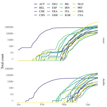
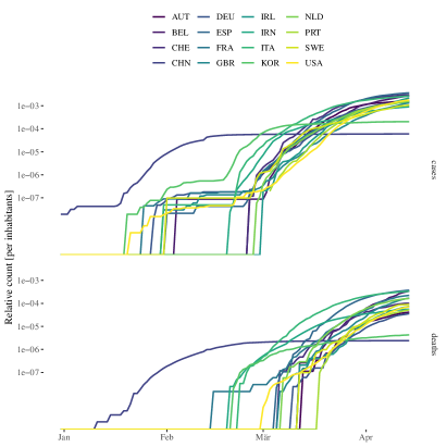
Figure 1: Case and death counts of selected countries. Both in absolute (left) and relative (right), i.e. per inhabitants, terms.

Figure 1 shows the total cumulative case and death counts of selected countries. These countries are among the eight most effected countries in terms of absolute and relative deaths. In the following, I will focus on relative counts as these are arguably more meaningful when comparing different countries – which could differ widely in terms of population size.

Assumption 1.

Death counts are more reliable than case counts.

By Assumption 1 analysis will start from relative cumulative death counts $d_{t}$ in the following. Furthermore, in order to facilitate country comparisons, dates are shifted relative to the first day that relative death counts exceed a threshold $\theta$ of $1,2,4$ or $8$ deaths per million inhabitants respectively, i.e. $t=0$ is defined such that $d_{t}\geq\theta$ for $t\geq 0$ and $d_{t}<\theta$ for $t<0$. Figure 2 shows the resulting time course of relative case and death counts. Aligning dates in this fashion shows that several countries exhibit similar time courses, e.g. Belgium and Spain or China and South Korea. As shown in the supplementary Figure S1 the remaining country specific differences can be explained by differences in growth rates. Re-scaling time according to the estimated doubling time indeed leads to a data collapse as complete as often observed in physical systems exhibiting scaling laws [11].

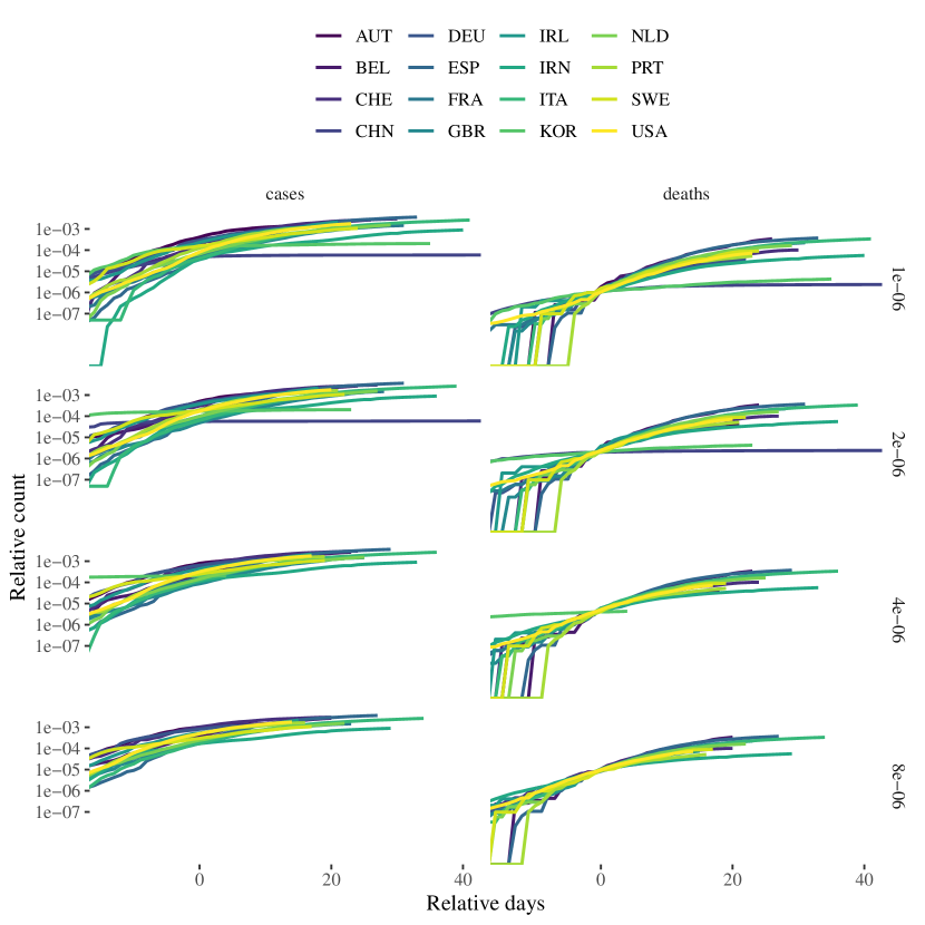
Figure 2: Relative case and death counts of selected countries. Dates are aligned relative to the first day that relative death counts exceed one (top) or ten (bottom) per million respectively.

Here, these differences in the precise temporal dynamics of epidemic growth are not required. Instead, the relation between relative death and case counts is considered. While relative death counts exhibit similar time courses the corresponding relative case counts $c_{t}$ are more variable when aligned in the same fashion, i.e. relative to the first day that $d_{t}$ exceeds a given threshold. As I will argue now, most of this variability can be explained with two readily interpretable parameters.

Assumption 2.

There is a well defined country specific delay between reported cases and deaths.

Figure 2 suggests that relative case counts are not aligned as some countries, e.g. Germany, systematically lead the counts reported in other countries, e.g. Italy. Such a difference could mean that individuals survive longer, e.g. due to differences in medical care, until they eventually. It could also just reflect reporting delays due to bureaucratic reasons. In any case, it is clearly the case that individuals die not immediately, but some days after they had been tested positive previously.

2.1 Case fatality rate

This delay also needs to be taken into account when estimating the case fatality rate (CFR). Commonly the CFR is defined as $\mathrm{cfr}=\frac{d_{t}}{c_{t}}$. Not surprisingly this estimate is highly variable and changes systematically over time, especially at the beginning of an epidemic. The observation captured in Assumption 2 also explains the surprisingly low CFRs initially announced in Austria and Germany where reported death counts are simply some days older compared to other countries!

Thus, taking into account that individuals that had been tested positive will usually not die on the same day but after some delay $\tau$ (if at all), I define

$$\mathrm{cfr}_{\tau} =\frac{d_{t}}{c_{t-\tau}}\;,$$ (1)

i.e. comparing current death with previous case counts.

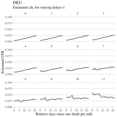
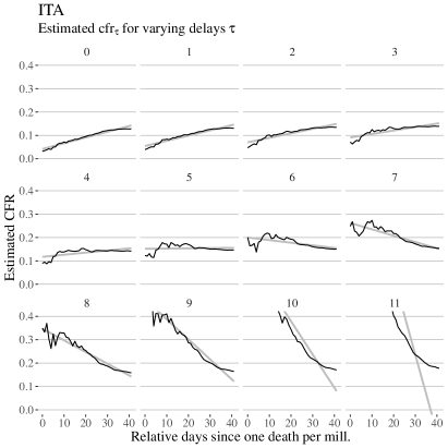
Figure 3: Estimated CFR $\mathrm{cfr}_{\tau}$ for Germany (left) and Italy (right) using different delays of $\tau=0,\ldots,11$ days. Note that in each case, there exists a characteristic delay such that estimates are almost constant over time. Further note that estimates for all delays will eventually converge to the same final value when enough data are available.

Figure 3 shows the CFRs estimated for Germany and Italy in this fashion, i.e. for different delays $\tau$. The estimate using $\tau=0$ rises over time simply reflecting that due to the reporting delay death counts have not yet caught up with the exponentially growing case counts. Interestingly, for each country there exists a characteristic delay at which the estimated CFRs are essentially constant. Thus, reflecting the hypothesized delay between reported cases and deaths.

This delay can either be estimated by visual inspection or by fitting a linear model on each delay and picking the one with minimal absolute slope. Figure 3 shows the delays $\tau$ and corresponding CFRs $\mathrm{cfr}_{\tau}$, i.e. the median CFR value at this delay, estimated for each country in this fashion. In order to fully relate the observed case with death counts an additional, and stronger, assumption is needed.

Assumption 3.

The true case fatality rate is the same for all countries.

While Assumption 3 ignores medical, demographic and other differences between countries, I believe it unlikely that the CFR is very different across different countries. In the end, its the same type of virus spreading in all countries. This suggests that differences in estimated CFRs simply reflect differences in the ability of countries to actually observe all infected individuals, i.e. due to more or less effective tracking and testing procedures. To illustrate this effect, a true CFR of $1\%$ is assumed in the following. This is consistent with current knowledge and had also been used in other studies [4]. Just from the estimated values any CFR below the minimum of all estimates (about $2\%$ found for Austria and South Korea) and above $0.1\%$ (which would imply an observed fraction above one for Belgium) is compatible with the data.

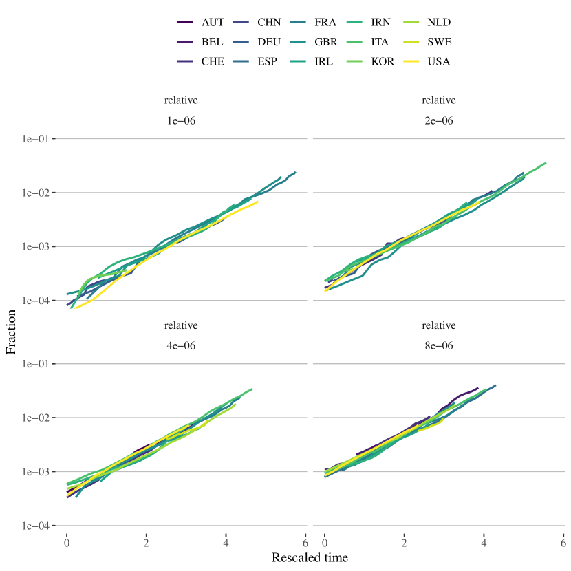
Figure S2: As Figure 5, but time is additionally re-scaled to match local growth rate of the epidemics.

Figure 4 shows the country specific estimates of reporting delay, CFR and fraction of observed cases (assuming a true CFR of $1\%$) obtained in this fashion. In turn, Figure 5 shows the implied relative case counts when shifted by the estimated delays and scaled to reflect the unobserved fraction of cases for each country. Notably, these implied counts all align nearly as good as the death counts in Figure 2 (right panel) even though the initial threshold was based on the deaths counts alone. The supplementary Figure S2 shows that this holds also when re-scaling time according to the growth rate of deaths. Overall, the collapse of implied case dynamics convincingly illustrates that the relation between case and death counts is fully and reliably captured by two parameters – compatible with three reasonable assumptions.

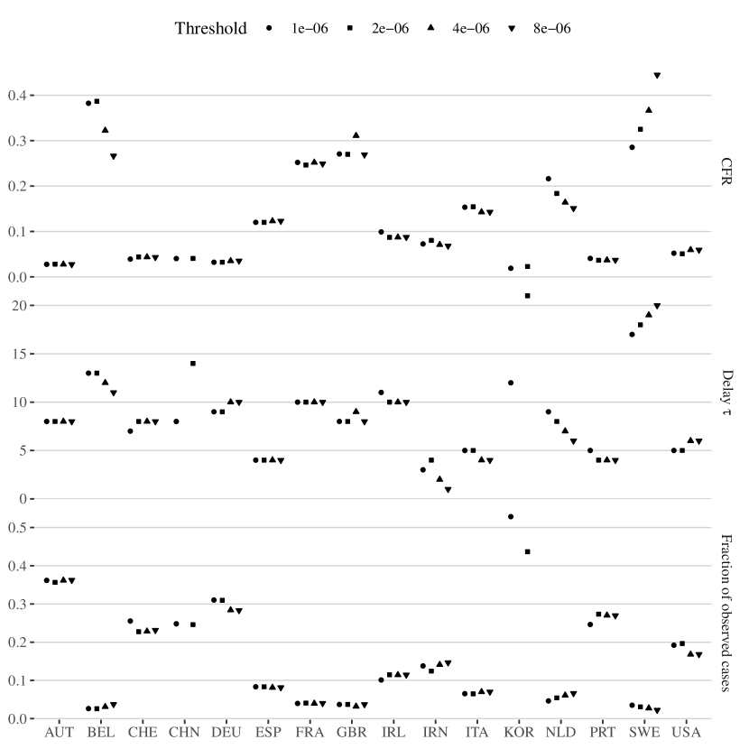
Figure 4:

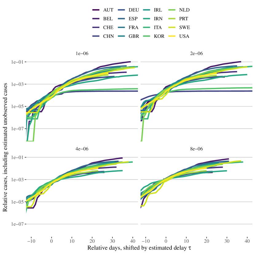
Figure 5:

3 Discussion

In reality, an additional delay between an infection and its corresponding positive test result can be assumed. Therefore, the fraction of observed cases will be even lower than obtained by the analysis above. Unfortunately, assuming a sufficiently flexible model for the growth of the actual cases already the CFR and the fraction of observed cases, let alone an additional delay, are not jointly identifiable.

3.1 Epidemic modeling

The basic SIR model [10], assumes that an infection unfolds when susceptible (S) individuals become infected (I) – which in turn infect further susceptible individuals. Finally, infected individuals recover (R) (or die) and are no longer susceptible. In continuous time, the dynamics can be described by the following system of ordinary differential equations (ODEs):

$$\frac{dS}{dt} =-\beta\frac{I_{t}}{N}S_{t}$$

$$\frac{dI}{dt} =\beta\frac{I_{t}}{N}S_{t}-\gamma I_{t}$$

$$\frac{dR}{dt} =\gamma I_{t}$$

where $N\equiv S_{t}+I_{t}+R_{t}$ is constant over time. Model parameters are

• the infection rate $\beta$

• and the recovery rate $\gamma$.

In this model, the average time of infection is $\gamma^{-1}$ giving rise to a basic reproduction number of $R_{0}=\beta\gamma^{-1}$.

SIR models and extensions are widely used in epidemic modeling. The have also been applied to the understand the dynamics of the ongoing Covid-19 pandemic [9, 2, 7, 13]. In particular, models including the possibility of unobserved cases or including a reporting delay have been developed. Within the SIR framework, both effects can be included in several ways, most easily by assuming that observed cumulative infections are simply a fraction $\alpha\in[0,1]$ of previous total infections $I_{t}+R_{t}$, i.e. $\alpha(I_{t-\tau}+R_{t-\tau})$. A more elaborate attempt instead considers more detailed dynamics of the form

$$\frac{dS}{dt} =-\beta_{I}\frac{S_{t}}{N}I_{t}-\beta_{O}\frac{S_{t}}{N}O_{t}-\beta_{U}\frac{S_{t}}{N}U_{t}$$

$$\frac{dI}{dt} =\beta_{I}\frac{S_{t}}{N}I_{t}+\beta_{O}\frac{S_{t}}{N}O_{t}+\beta_{U}\frac{S_{t}}{N}U_{t}-\gamma_{I}I_{t}$$

$$\frac{dO}{dt} =\alpha\gamma_{I}I_{t}-\gamma_{R}O_{t}$$

$$\frac{dU}{dt} =(1-\alpha)\gamma_{I}I_{t}-\gamma_{R}U_{t}$$

$$\frac{dR}{dt} =\gamma_{R}(O_{t}+U_{t})$$

where a fraction $\alpha$ of infected individuals $I_{t}$ is observed ($O_{t}$) after an initial delay $\frac{1}{\gamma_{I}}$. In any case, whether observed or not, individuals recover (or die) after an additional delay. In general, the infection rates $\beta_{I},\beta_{O},\beta_{U}$ could be different for initial infections and observed vs unobserved cases.

In addition, mitigation measures, e.g. social distancing, can be easily included by assuming that $\beta$’s are functions of time. E.g. [2] assumes one or several (soft) step functions where $\beta$ drops after measures have been implemented. Unfortunately, as we show now a model including a time-varying $\beta$ as well as unobserved cases is not identifiable. For simplicity, consider the above model with $\beta_{I}=\beta_{O}=\beta_{U}=:\beta$. Then, new infections arise with intensity $\beta\frac{S_{t}}{N}(I_{t}+O_{t}+U_{t})$ which in turn translate into observed cases with intensity $\alpha\gamma_{I}I_{t}$. Now assume a second model with $\alpha^{\prime}=1>\alpha$ which nevertheless exhibits the same dynamics with an additional time shift $\tau$. By using a time varying $\beta^{\prime}(t)$ such that

$$\beta^{\prime}(t) =\alpha\beta\frac{S_{t+\tau}}{S^{\prime}_{t}}$$

we obtain exactly the same number of observed cases, i.e. $O^{\prime}_{t-\tau}=O_{t}$. Note that as $\alpha^{\prime}>\alpha$, we have that $S_{t}<S^{\prime}_{t-\tau}$ and $S_{t}$ is a sigmoidal function of time due to the SIR dynamics. Furthermore, when the population is large, i.e. $N\gg 1$ and $S_{0}\approx N$ the resulting $\beta^{\prime}(t)$ is mostly driven by the drop in $S_{t+\tau}$ as compared to the much smaller change in $S^{\prime}_{t}$. Indeed, Figure 6 shows the dynamics of the above model with $\beta=0.3,\gamma_{I}=\gamma_{R}=\frac{2}{10}$, $\alpha=0.1$ starting from $(N=10^{8},1,0,0,0)$. In turn, assuming $\alpha^{\prime}=1$ and $\tau=5$, the time varying infectivity $\beta^{\prime}(t)$ is approximated by the best-fitting logistic sigmoid of the form $\beta_{1}+(\beta_{2}-\beta_{1})\sigma(\frac{t-\tau}{T})$. Note that the number of observed cases is identical, just shifted by $\tau$, whereas the final fraction of susceptible individuals is vastly different. Indeed, in the first case the epidemic is stopped by group immunity whereas in the second case effective mitigation measures are imposed. Correspondingly, police implications would be vastly different in the two situations even though they are observationally indistinguishable.

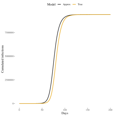
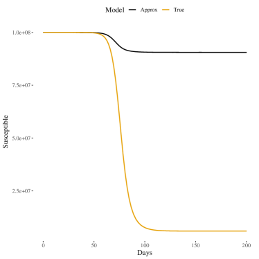
Figure 6: Total cumulative observed infections and number of susceptible individuals in two simulated model with observation fractions $\alpha=0.1$ (true), $\alpha^{\prime}=1$ and time shift $\tau=5$ (approx). In the second model, the epidemic is stopped due to mitigation measures which are modeled via $\beta^{\prime}(t)$ as explained in the main text.

3.2 Implications

Instead of detailed modeling of epidemic dynamics, which is further complicated due policy actions requiring flexible models with delicately chosen parameters, the present analysis is based on visual inspection of the reported data. Overall, relative case and deaths counts (observed for country $c$) seem to be related as follows:

$$d^{c}_{t} =\mathrm{cfr}\cdot a^{c}_{t-{\tau^{c}}}$$

$$c^{c}_{t} =\alpha^{c}\cdot a_{t}$$

where $a^{c}_{r}$ denotes the actual infections a fraction $\alpha^{c}\in[0,1]$ is observed. A suitable reporting delay $\tau^{c}$ can be estimated by visual inspection of the data, but again the fraction of observed cases $\alpha^{c}$ and CFR $\mathrm{cfr}$ are not jointly identifiable if there exist sets of parameters such that $a^{\prime}_{t-{\tau}}=\alpha a_{t}$, as is the case for dynamic SIR type models. In the end, any epidemic modeling implicitly or explicitly chooses a parametric form for the latent growth process $a_{t}$ and will not be identified if sufficiently flexible. Yet, assumption three of a constant CFR across all countries allows to derive

1. a range of values consistent among all countries,

2. as well as recover the corresponding fraction of observed cases in each country.

Thereby, assuming a reasonable true CFR value, i.e. from the model implied range $0.1\%$ to $2\%$ which is also consistent with current knowledge, and using the estimated delay, the actual case numbers can be reconstructed. Figure 7 shows the resulting actual relative infection counts across several countries. Note that despite the simplicity of this analysis, the estimated numbers compare favorable [4]. Indeed, I would rather trust these even more as they do not rely on complex modeling assumptions but follow from visual inspection of the data.

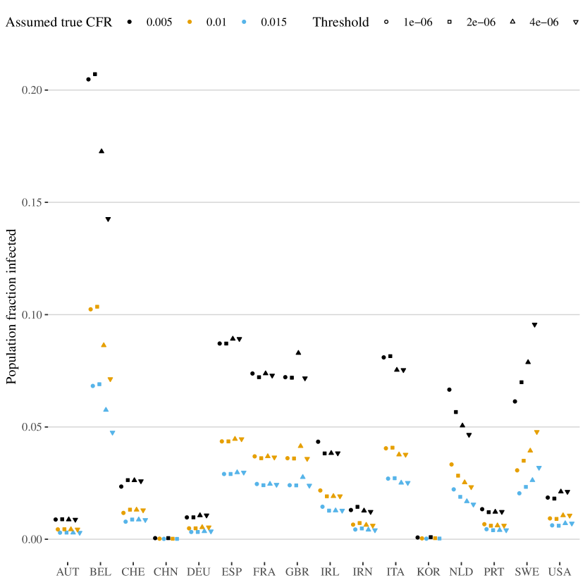
Figure 7: Estimated fraction of population already infected assuming a reasonable range of true CFRs.

Overall, I have illustrated that much of the variability between observed case and deaths counts between different countries can be explained by two parameters. Namely, the reporting delay $\tau$ and the fraction of observed cases. Especially the reporting delay exhibits crucial differences between countries and needs to be taken into account when comparing data and planning actions. In particular, containment is challenging when long incubation times are involved [1] but a combination of case tracing and isolation policies could be effective [5, 6]. Thus, detailed epidemic modeling is certainly needed in order to judge the effectiveness of current mitigation measures across different countries [4, 2]. On the other hand, important parameters need to fixed based on additional knowledge as they cannot be identified within sufficiently flexible models. In the end, data analysis and detailed modeling alone only gets us only that far and more extensive testing is urgently needed to obtain reliable knowledge about the current progression of the Covid-19 pandemic.

Supplement A Data collapse by re-scaling time

Aligning the data as in Figure 2 still shows country-specific differences in the temporal course of epidemic spreading. Much of this difference can be attributed to the speed at which the epidemic spreads in different countries. Estimating the local growth rate of deaths $\frac{d\log d_{t}}{dt}$ by the three day running average of observed changes $\log d_{t+1}-\log d_{t}$, relative time, i.e. relative to the threshold of total deaths reached, is re-scaled to match local growth rates. Figure S1 shows the resulting data collapse for $d_{t}$ and the corresponding $c_{t}$ dynamics.

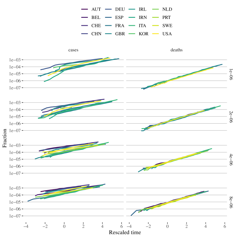
Figure S1: Aligned data as in Figure 2, but time is additionally re-scaled to match local growth rate of the epidemics.

Further, taking the estimated relation between cases and deaths via CFR and country specific delays into account an almost complete data collapse for the cases is obtained. Not that as in the main text, data are aligned according to relative death counts only. Furthermore, the temporal re-scaling is based on the estimated growth rate from the death counts as well. Yet, shifting and scaling case data according to the estimated country specific delay and fraction of observed cases leads to an almost complete data collapse as well.

Supplement B NY Times style figures

As individual countries can be hard to identify in Figures 2 and 5, the NY Times featured panel views where each country is highlighted above a background of all countries. Here, I provide similar figures for relative death and case counts using a threshold of two deaths per million inhabitants.

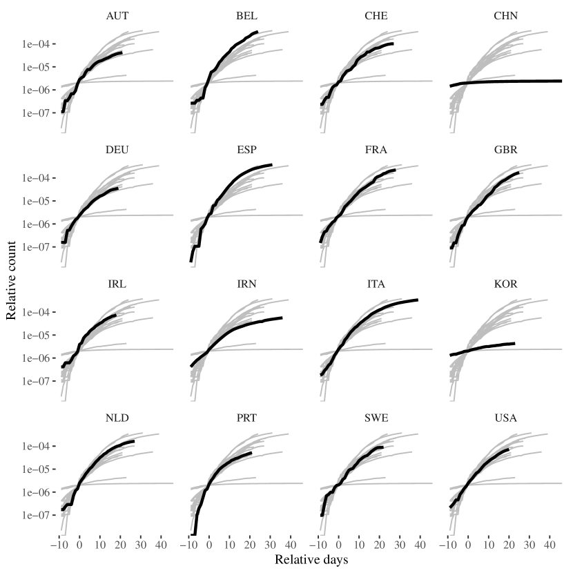
Figure S3: Details of aligned relative death counts for threshold of two deaths per million.

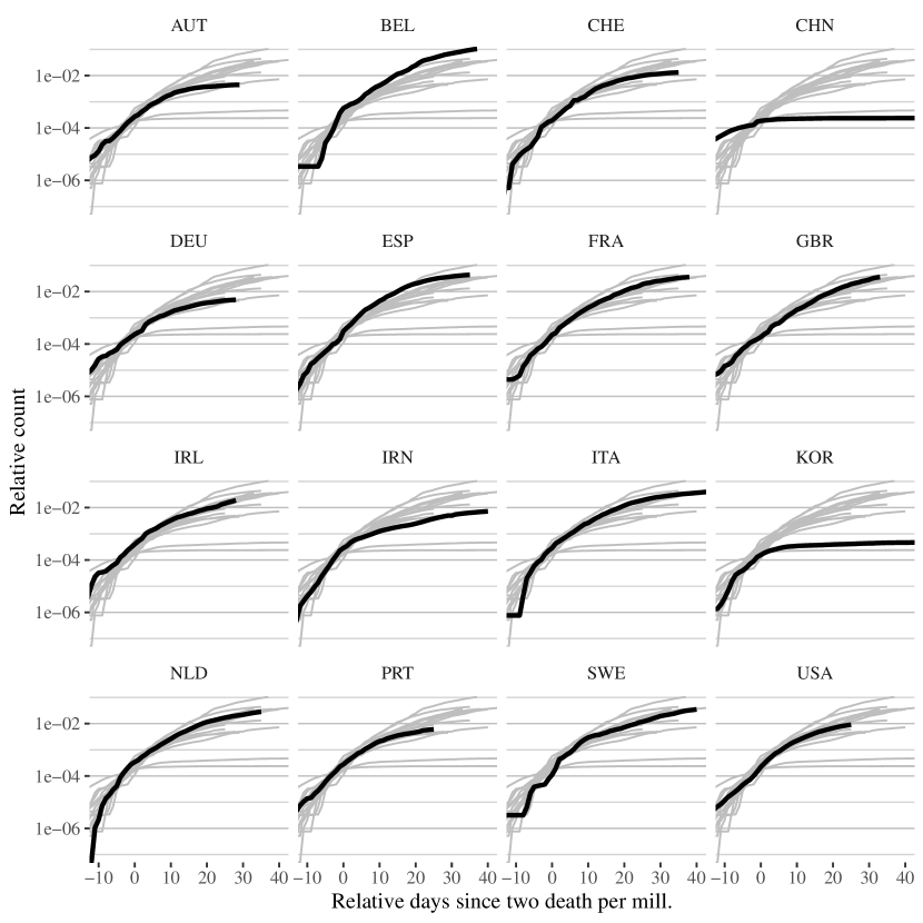
Figure S4: Details of aligned and adjusted case counts for threshold of two deaths per million.

Supplement C Uncertainty estimates from SIR model

Note that an SIR model already includes a natural delay between infections and recovery (or death). Indeed, the total number of cases is given by $C_{t}=I_{t}+R_{t}$ while the cumulative death toll is obtained as $\mathrm{cfr}R_{t}$, i.e. modeling that a fraction of individuals does not recover but dies instead. Assuming that only a fraction $\alpha$ of cases is observed, the model is estimated with the following sampling distribution

$$C^{\mathrm{obs}}_{t+1}-C^{\mathrm{obs}}_{t} \sim\mathrm{NegativeBinomial}\left(\alpha\frac{dC^{\mathrm{model}}_{t}}{dt},\phi_{C}\right)$$

$$D^{\mathrm{obs}}_{t+1}-D^{\mathrm{obs}}_{t} \sim\mathrm{NegativeBinomial}\left(\mathrm{cfr}\frac{dR^{\mathrm{model}}_{t}}{dt},\phi_{D}\right)\;.$$

Thus, observed daily changes are related to the model implement changes via an over-dispersed Poisson aka negative binomial distribution. Figure S5 shows the resulting estimates assuming $\beta_{t}=\beta_{1}+(\beta_{2}-\beta_{1})\sigma(\frac{t-\tau}{T})$ and $\mathrm{cfr}=1\%$. The SIR model assuming a single change point in the infectivity, via the logistic sigmoid $sigma(\cdot)$ in $\beta_{t}$ reflecting the implementation of social distancing is clearly able to capture the epidemic dynamics. Yet, parameter uncertainties, especially about the reporting delay can be large.

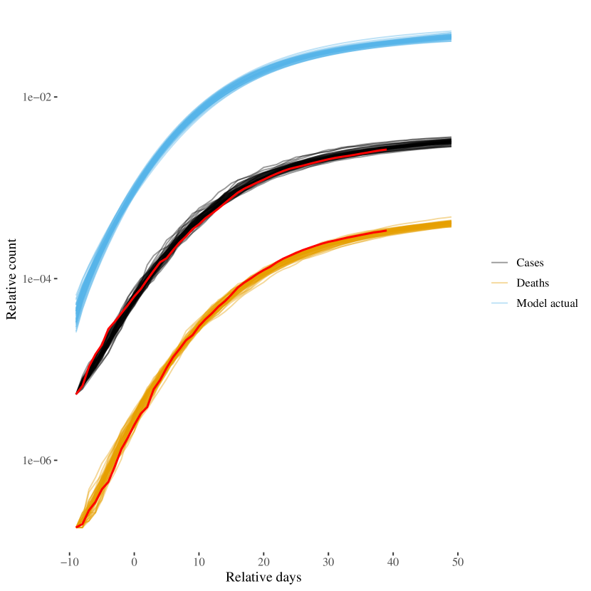
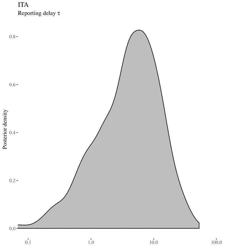
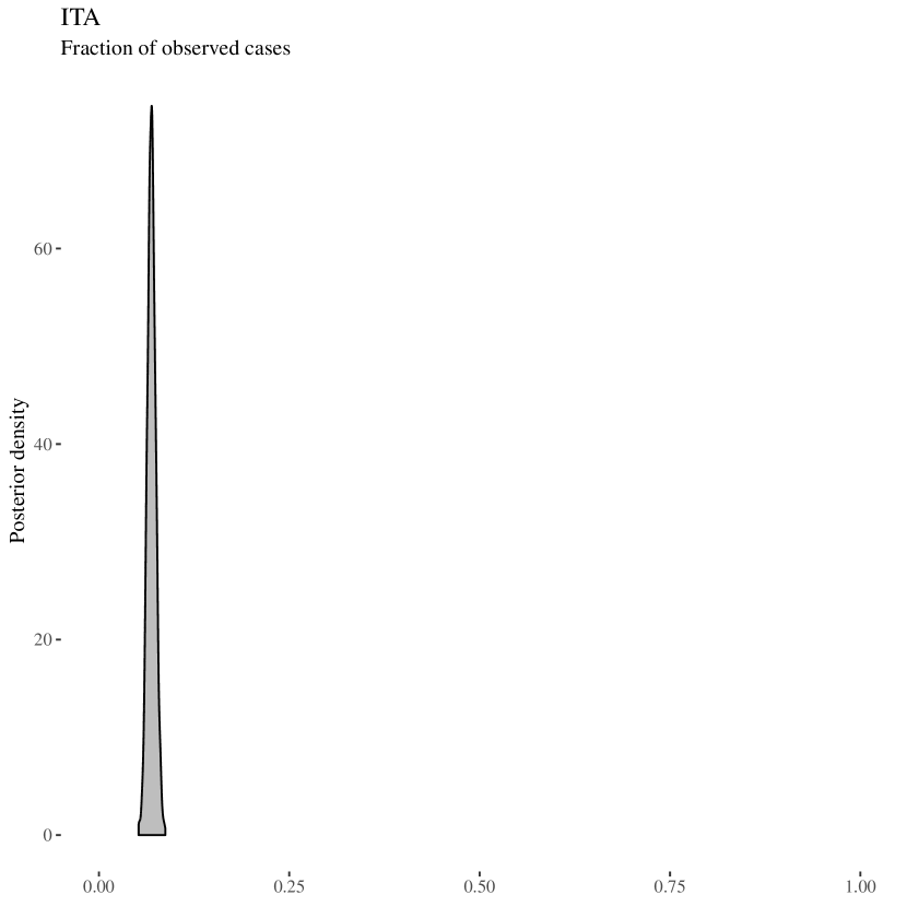
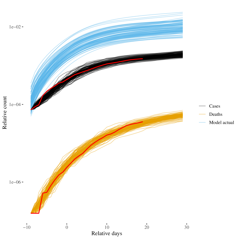
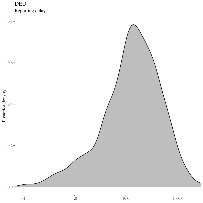
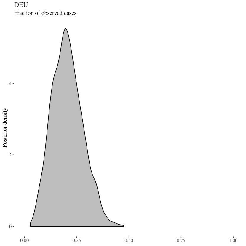
Figure S5: Model predictions and estimated parameters from SIR model fitted to data from Italy (top) and Germany (bottom).

Bayesian estimates have been carried out using Stan (full code available from my https://github.com/bertschi/Covid repository) and using weakly informative broad normal or student-t prior distributions on all parameters.

References

- [1] W. Bock, B. Adamik, M. Bawiec, V. Bezborodov, M. Bodych, J. P. Burgard, T. Goetz, T. Krueger, A. Migalska, B. Pabjan, T. Ozanski, E. Rafajlowicz, W. Rafajlowicz, E. Skubalska-Rafajlowicz, S. Ryfczynska, E. Szczurek, and P. Szymanski. Mitigation and herd immunity strategy for covid-19 is likely to fail. medRxiv, 2020.
- [2] J. Dehning, J. Zierenberg, F. P. Spitzner, M. Wibral, J. P. Neto, M. Wilczek, and V. Priesemann. Inferring covid-19 spreading rates and potential change points for case number forecasts, 2020.
- [3] N. M. Ferguson, D. Laydon, G. Nedjati-Gilani, N. Imai, K. Ainslie, M. Baguelin, S. Bhatia, A. Boonyasiri, Z. Cucunubá, G. Cuomo-Dannenburg, A. Dighe, I. Dorigatti, H. Fu, K. Gaythorpe, W. Green, A. Hamlet, W. Hinsley, L. C. Okell, S. van Elsland, H. Thompson, R. Verity, E. Volz, H. Wang, Y. Wang, P. G. Walker, C. Walters, P. Winskill, C. Whittaker, C. A. Donnelly, S. Riley, and A. C. Ghani. Impact of non-pharmaceutical interventions (NPIs) to reduce COVID-19 mortality and healthcare demand. Imperial College COVID-19 Response Team, March 2020.
- [4] S. Flaxman, S. Mishra, A. Gandy, H. J. T. Unwin, H. Coupland, T. A. Mellan, H. Zhu, T. Berah, J. W. Eaton, P. N. P. Guzman, N. Schmit, L. Cilloni, K. E. C. Ainslie, M. Baguelin, I. Blake, A. Boonyasiri, O. Boyd, L. Cattarino, C. Ciavarella, L. Cooper, Z. Cucunubá, G. Cuomo-Dannenburg, A. Dighe, B. Djaafara, I. Dorigatti, S. van Elsland, R. FitzJohn, H. Fu, K. Gaythorpe, L. Geidelberg, N. Grassly, W. Green, T. Hallett, A. Hamlet, W. Hinsley, B. Jeffrey, D. Jorgensen, E. Knock, D. Laydon, G. Nedjati-Gilani, P. Nouvellet, K. Parag, I. Siveroni, H. Thompson, R. Verity, E. Volz, C. Walters, H. Wang, Y. Wang, O. Watson, P. Winskill, X. Xi, C. Whittaker, P. G. Walker, A. Ghani, C. A. Donnelly, S. Riley, L. C. Okell, M. A. C. Vollmer, N. M. Ferguson, and S. Bhatt. Estimating the number of infections and the impact of non-pharmaceutical interventions on COVID-19 in 11 european countries. Imperial College COVID-19 Response Team, March 2020.
- [5] C. Fraser, S. Riley, R. Anderson, and N. Ferguson. Factors that make an infectious disease outbreak controllable. Proc Natl Acad Sci USA, 101(16):6146–6151, 2004.
- [6] R. Kubinec. A retrospective Bayesian model for measuring covariate effects on observed covid-19 test and case counts. SocArXiv, April 2020.
- [7] R. Li, S. Pei, B. Chen, Y. Song, T. Zhang, W. Yang, and J. Shaman. Substantial undocumented infection facilitates the rapid dissemination of novel coronavirus (sars-cov2). Science, 2020.
- [8] J. Lourenco, R. Paton, M. Ghafari, M. Kraemer, C. Thompson, P. Simmonds, P. Klenerman, and S. Gupta. Fundamental principles of epidemic spread highlight the immediate need for large-scale serological surveys to assess the stage of the sars-cov-2 epidemic. medRxiv, 2020.
- [9] B. F. Maier and D. Brockmann. Effective containment explains sub-exponential growth in confirmed cases of recent covid-19 outbreak in mainland china, 2020.
- [10] M. Newman. Networks. Oxford University Press, 2nd edition, 2018.
- [11] H. E. Stanley. Scaling, universality, and renormalization: Three pillars of modern critical phenomena. Rev. Mod. Phys., 71:S358–S366, Mar 1999.
- [12] W. Yang, D. Zhang, L. Peng, C. Zhuge, and L. Hong. Rational evaluation of various epidemic models based on the covid-19 data of china. medRxiv, 2020.
- [13] S. Zhao and H. Chen. Modeling the epidemic dynamics and control of covid-19 outbreak in china. medRxiv, 2020.