The Impact of Heterogeneity and Geometry
on the Proof Complexity of Random Satisfiability

Abstract

Satisfiability is considered the canonical NP-complete problem and is used as a starting point for hardness reductions in theory, while in practice heuristic SAT solving algorithms can solve large-scale industrial SAT instances very efficiently. This disparity between theory and practice is believed to be a result of inherent properties of industrial SAT instances that make them tractable. Two characteristic properties seem to be prevalent in the majority of real-world SAT instances, heterogeneous degree distribution and locality. To understand the impact of these two properties on SAT, we study the proof complexity of random $k$-SAT models that allow to control heterogeneity and locality. Our findings show that heterogeneity alone does not make SAT easy as heterogeneous random $k$-SAT instances have superpolynomial resolution size. This implies intractability of these instances for modern SAT-solvers. On the other hand, modeling locality with an underlying geometry leads to small unsatisfiable subformulas, which can be found within polynomial time.

A key ingredient for the result on geometric random $k$-SAT can be found in the complexity of higher-order Voronoi diagrams. As an additional technical contribution, we show an upper bound on the number of non-empty Voronoi regions, that holds for points with random positions in a very general setting. In particular, it covers arbitrary ${\mathfrak{p}}$-norms, higher dimensions, and weights affecting the area of influence of each point multiplicatively. Our bound is linear in the total weight. This is in stark contrast to quadratic lower bounds for the worst case.

1 Introduction

Propositional satisfiability (SAT) is arguably among the most-studied problems for both theoretical and practical research. Nonetheless, the gap between theory and practice is huge. In theory, SAT is the prototypical hard problem and hardness of other problems is shown via reductions from SAT. Achieving even a running time of $O(2^{cn})$ for any $c<1$ and $n$ variables would be a major breakthrough and a somewhat surprising one at that. On the contrary, reductions to SAT are used to solve various problems appearing in practice, as state-of-the-art SAT solvers can easily handle industrial instances with millions of variables.

This theory–practice gap does not come from the lack of a sufficiently precise theoretical analysis of modern SAT solvers. They are actually provably slow on most instances, i.e., drawing an instance uniformly at random yields a hard instance with probability tending to $1$ for $n\to\infty$, if the clause-variable ratio is not too low or way too high [9, 21]. Instead, the discrepancy comes from the fact that industrial instances have properties that make them easier than worst-case instances. In 2014, Vardi [59] wrote that “we have no understanding of why the specific sets of heuristics employed by modern SAT solvers are so effective in practice” and that we need this understanding to successfully advance SAT solving further.

In recent years, scientists have been studying properties of industrial SAT instances to gain this understanding. By modeling SAT instances as graphs, e.g., with edges indicating inclusion of variables in clauses, one can benefit from the extensive research conducted in the field of network science. Two properties commonly observed in real-world networks are heterogeneity and locality. Heterogeneity refers to the degree distribution, meaning that vertices have strongly varying degrees. In fact, one usually observes a heavy-tailed distribution with many vertices of low degree and few vertices of high degree. A common assumption is a power-law distribution [60], where the number of vertices of degree $k$ is roughly proportional to $k^{-\beta}$. The constant $\beta$ is called the power-law exponent. Locality refers to the fact that edges tend to connect vertices that are close in the sense that they remain well connected even when ignoring their direct connection. This can also be seen as having strong community structures, with high connectivity within communities and loose ties between communities.

With respect to these two properties, industrial SAT instances are similar to real-world networks. In many cases, the variable frequencies are heterogeneous [1] and there is a high level of locality [2]. The latter is often measured in terms of modularity. Inspired by network science, researchers have studied models that resemble industrial instances with respect to these properties. Particularly, Ansótegui et al. [3] introduced a power-law SAT model for heterogeneous instances, which has been theoretically studied in terms of satisfiability thresholds [34, 35, 33]. A different model with heterogeneous degree distributions has been studied by Cooper et al. [22], Ansótegui et al. [4], and Omelchenko and Bulatov [52]. Moreover, Giráldez-Cru and Levy [40] introduced a model in which variable weights lead to heterogeneity while an underlying geometry facilitates locality. Comparing this to network models, the former model [3] is the SAT-variant of Chung-Lu graphs [20, 19]. The latter [40] is based on the popularity-similarity model [53], which is closely related to hyperbolic random graphs [44] and geometric inhomogeneous random graphs [18].

Besides serving as somewhat realistic benchmarks for SAT competitions [39], these SAT models can be used to study solver behavior depending on heterogeneity and locality. One can experimentally observe that a high level of heterogeneity improves the performance of SAT solvers that also perform well on industrial instances [3, 13]. Moreover, locality seems very beneficial as solvers appear to implicitly use the locality of a given instance [40]. This coincides with the findings of experiments on actual industrial instances that show that the locality (measured using modularity) of an instance is a good predictor for solver performance [51, 62, 63].

Up to date, there are no theoretical results supporting these experimental observations. On the contrary, it has been shown that instances generated by the community attachment model [38], which enforces a community structure, are hard for modern SAT solvers [49]. With this paper, we provide a theoretical foundation that matches the observations in practice by studying the proof complexity of $k$-SAT instances (for constant $k$) drawn from the power-law SAT model, and from a very general model with underlying geometry. The former was introduced by Ansótegui et al. [3], the latter is a generalization of the geometric model by Giráldez-Cru and Levy [40] in the same way as geometric inhomogeneous random graphs [18] are a generalization of hyperbolic random graphs [44]. Our findings are that heterogeneous instances are hard asymptotically almost surely in that modern SAT solvers require superpolynomial or even exponential running time to refute unsatisfiable instances. On the contrary, instances with a high level of locality facilitated by an underlying geometry are a. a. s. easy to solve. Our results focus on unsatisfiable instances, i.e., on the case where a solver has to prove that no satisfying assignment exists. This is typically much harder than finding a satisfying assignment, making the unsatisfiable regime arguably more relevant. Besides these results on SAT, we provide insights on the complexity of weighted higher-order Voronoi diagrams in higher dimensions, which is of independent interest.

The power-law and geometric models both mimic specific properties observed in industrial instances while trying to make as little additional assumptions as possible. Though this makes the resulting instances arguably more realistic than, e.g., instances drawn uniformly at random, we want to stress that even the geometric model is far from a perfect representation of industrial instances. Thus, our results do not claim to completely explain the efficiency of modern SAT solvers on industrial instances. However, to the best of our knowledge, we provide the first theoretical result that links a high level of locality to provably more tractable instances, which we believe to be a first step towards closing the theory–practice gap.

Outline

We state and discuss our main results and technical contributions in Section 2. Formal definitions are in Section 3. A short outline of our core arguments is in Section 4, followed by the formal proofs: lower bounds for the power-law model in Section 5, upper bounds on the complexity of Voronoi diagrams in Section 6, and upper bounds for the geometric SAT model in Section 7. To not distract from the core arguments, results we use that were either known before or are straight-forward to prove are outsourced to Appendix A.

2 Results, Technical Contribution, Discussion

In this section, we state our results and discuss the contribution, also in context to previous results. To make the results understandable, we briefly discuss, e.g., the probability distributions over SAT formulas we study. These are short and not meant to be formal definitions. For complete definitions, see Section 3.

2.1 Power-Law SAT

The power-law SAT model has four parameters: the number of variables $n$, the number of clauses $m$, the number $k$ of variables appearing in each clause, and a power-law exponent $\beta$. To draw a formula, power-law weights with exponent $\beta$ are assigned to the variables and then each clause is generated independently by drawing $k$ variables without repetition using probabilities proportional to the weights. Each literal is negated with probability $1/2$.

To discuss our first main contribution, let $\Phi$ be a formula drawn from the power-law model with density at or above the satisfiability threshold, i.e., $\Phi$ is unsatisfiable at least with constant probability. We show that, although it is likely that $\Phi$ is unsatisfiable, it is highly unlikely that modern SAT solvers can figure that out in polynomial time. We prove this using resolution proof complexity.

Resolution is a refutation technique for propositional and first-order logic introduced by [24]. If an application of resolution steps leads to a contradiction, the formula is unsatisfiable. The sequence of resolved clauses then serves as a proof for unsatisfiability, also called a refutation of the formula. The resolution proof system exhibits a strong connection to modern Davis–Putnam–Logemann–Loveland (DPLL) and conflict-driven clause learning (CDCL) SAT solvers: DPLL is polynomially equivalent to tree-like resolution [58] and CDCL with unlimited restarts is polynomially equivalent to resolution [54, 7]. Thus, the minimum number of steps necessary to derive a contradiction also yields a lower bound on the running time of solvers simulating the same process. This number of steps is also called the resolution size of a formula, i. e. the minimum number of resolution steps necessary to arrive at a contradiction. Equivalently, the width of a resolution proof is the size of the largest clause appearing in the proof and the resolution width of a formula is the smallest width of any proof refuting that formula. Interestingly, a lower bound $w$ on the resolution width of a formula also implies a lower bound on its resolution size [9]: every resolution proof of a formula in $k$-CNF has size $\exp(\Omega((w-k)^{2}/n))$ and every tree-like resolution proof has size $2^{w-k}$.

We will show a lower bound for the resolution width of unsatisfiable formulas drawn from the power-law model. Our results translate to lower bounds on the resolution size and thus to matching lower bounds on the running time of conflict-driven clause learning (CDCL) solvers. For DPLL solvers, which use tree-like resolution, the bounds are even stronger. We only consider the resolution width of unsatisfiable instances. Thus, the probability bound we get is actually a conditional probability conditioned on instances being unsatisfiable. Note that our bound does not only hold above the satisfiability threshold, where a random formula $\Phi$ is a. a. s. unsatisfiable, but also at the threshold, where it is unsatisfiable with constant probability.

theoremmainone Let $\Phi$ be an unsatisfiable random power-law $k$-SAT formula with $n$ variables, $m\in\Omega(n)$ clauses, $k\geq 3$, and power-law exponent $\beta>\frac{2k-1}{k-1}$. Let $\Delta=m/n$ be large enough so that $\Phi$ is unsatisfiable at least with constant probability. Let $\varepsilon$, $\varepsilon_{1},\dots,\varepsilon_{3}$ be constants with $\varepsilon>0$, $\varepsilon_{1}=\frac{k-\varepsilon}{2}-1>0$, $\varepsilon_{2}=(k-\varepsilon)\cdot\frac{\beta-2}{\beta-1}-1>0$, and $0<\varepsilon_{3}<(\frac{k}{2}-1)\cdot\frac{\beta-2}{\beta-1}-1$. For the resolution width $w$ of $\Phi$, it holds a. a. s. that:

1. If $\beta\in\left(\frac{2k-1}{k-1},3\right)$ and $\Delta\in o\left(n^{\varepsilon_{2}}\right)$, then $w\in\Omega\left(n^{\varepsilon_{2}/\varepsilon_{1}}\Delta^{-1/\varepsilon_{1}}\right)$.

2. If $\beta=3$ and $\Delta\in o\left(n^{\varepsilon_{1}}/\log^{1+\varepsilon_{1}}n\right)$, then $w\in\Omega\left(n\cdot\Delta^{-1/\varepsilon_{1}}/\log^{1+1/\varepsilon_{1}}n\right)$.

3. If $\beta>3$ and $\Delta\in o\left(n^{\varepsilon_{1}}\right)$, then $w\in\Omega\left(n\cdot\Delta^{-1/\varepsilon_{1}}\right)$.

4. If $\beta>\frac{2k-2}{k-2}$ and $\Delta\in o\left(n^{\varepsilon_{3}}/\log^{\varepsilon_{3}}n\right)$, then $w\in\Omega\left(n\cdot\Delta^{-1/\varepsilon_{3}}\right)$.

Figure 1: Exponent of the bound (i) in Theorem 2.1. Dashed vertical lines show where the bound (iv) takes over.

The above lower bounds allow the density $\Delta$ to be super-constant (even polynomial), which is asymptotically above the satisfiability threshold. For the sake of simplicity, assume $\Delta$ to be constant in the following. Starting at the bottom (iii, iv), we get a linear bound for $w$ if $\beta$ is sufficiently large, i.e., greater than $3$ or $(2k-2)/(k-2)$. For $\beta=3$ (ii), the bound is still almost linear. Note that these results in particular imply exponential lower bounds on the resolution size and thus on the running time of CDCL and DPLL. For smaller $\beta$ (i), we get a polynomial bound for the width with exponent $\varepsilon_{2}/\varepsilon_{1}$; see Figure 1 for a plot with $\varepsilon$ close to $0$.

Interestingly enough, our bounds only hold for power law exponents $\beta>\frac{2k-1}{k-1}$. This is complemented by a previous result [34], which shows that the satisfiability threshold of power-law random $k$-SAT is at density $\Delta=\Theta(1)$ for power law exponents $\beta>\frac{2k-1}{k-1}$ and that asymptotically almost surely instances with constant constraint densities are trivially unsatisfiable for power law exponents $\beta<\frac{2k-1}{k-1}$. Thus, the resolution width is constant in the latter case.

Part iv of Theorem 2.1 is derived via lower bounds on the bipartite expansion of the clause-variable incidence graph of these instances. These results can be of independent interest for hypergraphs with edge size $k$ and for random $(0,1)$-matrices. Additionally, these expansion properties yield lower bounds for the clause space complexity, which in turn gives lower bounds on the tree-like resolution size of such formulas (Section 5.2). More precisely, this results in an exponential lower bound on the tree-like resolution size for $\beta>\frac{2k-3}{k-2}$. This is an improvement of the bound obtained via resolution width.

It is interesting to note that this result on the non-geometric model supports the claim that locality is a crucial factor for easy SAT instances. The lower bounds for the power-law model are solely based on the fact that every set of clauses covers a comparatively large set of variables. In other words, we only use that there are no clusters of clauses with similar variables, i.e., we explicitly use the lack of locality.

2.2 Geometric SAT

The geometric model has the following parameters: $n$, $m$, and $k$ have the same meaning as for the power-law model. Moreover, $w$ is a weight function assigning each variable $v$ a weight $w_{v}$ and $T$ is the so-called temperature that controls the strength of locality by varying the impact of the geometry. As underlying geometric space, we use the $d$-dimensional torus $\mathbb{T}^{d}=\mathbb{R}^{d}/\mathbb{Z}^{d}$ (see Section 3) equipped with a ${\mathfrak{p}}$-norm with ${\mathfrak{p}}\in\mathbb{N}^{+}\cup\infty$. To draw a formula, the variables and clauses are assigned random positions in $\mathbb{T}^{d}$. Then, for each clause, $k$ variables are drawn without repetition with probabilities depending on the variable weight and on the geometric distance between clause and variable. In the extreme case of $T=0$, each clause deterministically includes the $k$ closest variables (where closeness is a combination of geometric distance and weight), while increasing the temperature $T$ increases the probability for the inclusion of more distant variables. For $T\to\infty$, the model converges to uniform random SAT. Note that the weights are a parameter of the model and not drawn randomly. We have the following theorem, where $W$ denotes the sum of all variable weights. The condition on the weights is in particular satisfied by power-law distributed weights.

theoremGeometricSat Let $\Phi$ be a formula with $n$ variables and $m\in\Theta(n)$ clauses drawn from the weighted geometric model with ground space $\mathbb{T}^{d}$ equipped with a ${\mathfrak{p}}$-norm, temperature $T<1$, $W\in O(n)$, and $w_{v}\in O(n^{1-\varepsilon})$ for every $v\in V$ and any constant $\varepsilon>0$. Then, $\Phi$ contains a. a. s. an unsatisfiable subformula of constant size, which can be found in $O(n\log n)$ time.

To briefly explain how we prove this, consider a simplified version where variables and clauses are points in the Euclidean plane and each clause contains the $k$ variables geometrically closest to it (temperature $T=0$). Now consider the equivalence relation obtained by defining two points of the plane equivalent if and only if they have the same set of $k$ closest variables. The equivalence classes of this relation are the regions of the order-$k$ Voronoi diagram of the variable positions. With this connection, we can use upper bounds on the complexity of order-$k$ Voronoi diagrams [46] to prove the existence of small and easy to find unsatisfiable subformulas. We note that this result is of asymptotic nature. In particular for small densities, the number of variables $n$ has to be very large before the instances actually get as easy as stated in Theorem 2.2. Nevertheless, this results strongly suggests that an underlying geometry makes SAT instances more tractable.

To extend the above argument to the general statement in Theorem 2.2, we extend the complexity bounds for order-$k$ Voronoi diagrams in various ways; see next section for more details. Moreover, for non-zero temperatures, clauses no longer include exactly the $k$ closest variables but can, in principle, consist of any set of $k$ variables. However, we can show that, with high probability, a linear fraction of clauses behaves as in the $T=0$ case. We note that analyses of similar structures, such as hyperbolic random graphs, are often restricted to the simpler but less realistic $T=0$ case, e.g., [12, 11, 14, 48]. We believe that our analysis provides insights on the non-zero temperature case that can be helpful for such related questions.

We note that our results seem to contradict the results of Mull et al. [49], stating that (i) a strong community structure is not sufficient to have tractable SAT instances and that (ii) the community attachment model [38], which enforces a community structure, generates hard instances. However, at a closer look, this is not a contradiction at all. Though measuring the community structure, e.g., via modularity, is a good indicator for locality, the concept of locality goes deeper. If the instance can be partitioned such that there are strong ties within each partition and loose ties between partitions, then the instance has a strong community structure. However, to have a high level of locality, this concept has to hierarchically repeat on different levels of magnitude, i.e., there needs to be community structure within each partition and between the partitions. To state this slightly differently, consider locality based on a notion of similarity between objects (here: variables or clauses). In this paper, we use distances between random points in a geometric space as a measure for similarity, which gives us a continuous range of more or less similar objects. In contrast to that, in the above mentioned papers focusing on a flat community structure [38, 49], similarity is a binary equivalence relation: two objects are either similar or they are not.

2.3 Voronoi Diagrams

Consider a finite set of points, called sites, in a geometric space. The most commonly studied type of Voronoi diagram assumes the 2-dimensional Euclidean plane as ground space and has one Voronoi region for each site, containing all points closer to this site than to any other site. We deviate from this default setting in four ways: (i) We allow an arbitrary constant dimension $d$, where the ground space is the torus or a hypercube in $\mathbb{R}^{d}$. (ii) We consider the order-$k$ Voronoi diagram, which has for every subset $A$ of sites with $|A|=k$ a (possibly empty) Voronoi region containing all points for which $A$ are the $k$ nearest sites. The number of non-empty order-$k$ Voronoi regions is called the complexity of the diagram. (iii) The sites have multiplicative weights that scale the influence of the different sites. Without loss of generality, we assume the weights to be scaled such that the minimum is $1$. (iv) We allow the ${\mathfrak{p}}$-norm for arbitrary ${\mathfrak{p}}\in\mathbb{N}^{+}\cup\infty$.

theoremComplexityRandomVoronoiDiagram Let $S$ be a set of $n$ sites with minimum weight $1$, total weight $W$, and random positions on the $d$-dimensional torus equipped with a ${\mathfrak{p}}$-norm, for constant $d$. For every fixed $k$, the expected number of regions of the weighted order-$k$ Voronoi diagram of $S$ is in $O(W)$. The same holds for random sites in a hypercube.

To set this result into context, we briefly discuss previous work on the complexity of Voronoi diagrams in different settings. See the book by Aurenhammer et al. [6] for a general overview on Voronoi diagrams. To this end, we use the following theorem that relates the complexity in terms of Voronoi regions (which is what we are concerned with in this paper) with the complexity in terms of vertices.

theoremVoronoiComplVerticesRegions Let $S$ be a set of $n$ weighted sites in general position in $\mathbb{R}^{d}$ equipped with a ${\mathfrak{p}}$-norm. If the order-$k$ Voronoi diagram has $\ell$ vertices, then the order-$(k+d)$ Voronoi diagram has $\Omega(\ell)$ non-empty regions.

We note that, using insights from previous work, this theorem is not hard to prove. One basically has to generalize the result by Lê [45] bounding the number of $d$-spheres going through $d+1$ points in $d$-dimensional space to weighted sites, and then observe how the Voronoi diagram changes in the construction by Lee [46] for $d=2$, when going from order-$k$ to order-$(k+1)$. However, we are not aware of previous work stating this connection between vertices and non-empty regions in higher orders explicitly.

The four above-mentioned generalizations of the basic Voronoi diagram (higher dimension, higher order, multiplicative weights, and different ${\mathfrak{p}}$-norms) have all been considered before. However, to the best of our knowledge, not all of them together.

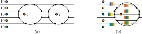
Figure 2: (a) Weighted Voronoi diagram (order-$1$) of the colored sites. Continuing the construction with $n/2$ high-weight sites on the left and $n/2$ low-weight sites towards the right yields $\Theta(n^{2})$ vertices (small black dots). Note that each vertex lies on the boundary of three regions and has thus equal weighted distance to its three closest sites. (b) The order-$3$ Voronoi diagram for the same sites (excluding one). The colored boxes indicate the three closet sites. The order-$1$ diagram is shown in the background. Each order-$1$ vertex lies in the interior of an order-$3$ region as it has equal weighted distance to its three closest sites. As at most two order-$1$ vertices share an order-$3$ region, we get $\Omega(n^{2})$ order-$3$ regions. Theorem 2.3 generalizes this observation.

Higher-order Voronoi diagrams have been introduced by Shamos and Hoey [57]. Lee [46] showed that the order-$k$ Voronoi diagram in the plane (unweighted with Euclidean metric) has complexity $O(k\,(n-k))$ (in terms of number of regions), which is linear for constant $k$. For the $1$- and $\infty$-norm, Liu et al. [47] improved this bound to $O(\min\{k\,(n-k),(n-k)^{2}\})$. Closely related to the $1$-norm, Gemsa et al. [37] showed similar complexity bounds for higher-order Voronoi diagrams on transportation networks of axis-parallel line segments. Bohler et al. [15] show an upper bound of $2k\,(n-k)$ for the much more general setting of abstract Voronoi diagrams. There, the metric is replaced by curves separating pairs of sites such that certain natural (but rather technical) conditions are satisfied. One obtains normal Voronoi diagrams when using perpendicular bisectors for these curves. This in particular shows that the $2k\,(n-k)$ bound on the number of regions in the order-$k$ Voronoi diagram holds for arbitrary ${\mathfrak{p}}$-norms in $2$-dimensional space and for the hyperbolic plane. As the hyperbolic plane is closely related to $1$-dimensional space with sites having multiplicative power-law weights [18], we suspect that the bound by Bohler et al. [15] also covers this case.

In general one can say that higher-order Voronoi diagrams of unweighted sites in $2$-dimensional space are well-behaved in that they have linear complexity. This still holds true for arbitrary ${\mathfrak{p}}$-norms. However, this picture changes for weighted sites or higher dimensions.

Voronoi diagrams with multiplicative weights were first considered by Boots [17] due to applications in economics. Beyond that, multiplicatively weighted Voronoi diagrams have applications in sensor networks [23], logistics [36] and the growth of crystals [25]. However, even in the most basic setting of 2-dimensional Euclidean space and order $1$, weighted Voronoi diagrams can have quadratic complexity [5] (in terms of number of vertices). This comes from the fact that Voronoi cells are not necessarily connected; see Figure 2a for the construction of Aurenhammer and Edelsbrunner [5] that proves the lower bound. With Theorem 2.3, and as illustrated in Figure 2, this implies that even the order-$3$ Voronoi diagram of weighted sites in 2-dimensional Euclidean space has a quadratic number of non-empty regions. As a special case, Theorem 2.3 shows that this complexity is only linear in the total weight for sites positioned randomly in the unit square. Moreover, this also implies that the number of vertices of the corresponding order-$1$ Voronoi diagram is linear. This nicely complements the result by Har-Peled and Raichel [42], who show that the expected complexity of order-$1$ Voronoi diagrams of sites in $2$-dimensional Euclidean space with random weights is $O(n\operatorname{polylog}n)$. Only recently, Fan and Raichel [32] showed that sites with weights chosen randomly form a constant-sized set of possible weights yield Voronoi diagrams with linear complexity. Moreover, more closely related, they show that the Voronoi diagram of sites with arbitrary weights and with random positions chosen in the unit square has linear complexity in expectation. We are not aware of any results concerning the complexity of Voronoi diagrams when combining multiplicative weights with higher dimension, higher order or other norms.

For higher dimensions, even normal (first order, unweighted) Voronoi diagrams in $3$-dimensional Euclidean space can have $\Theta(n^{2})$ [43, 56] vertices. Theorem 2.3 thus implies that the order-$4$ Voronoi diagram has a quadratic number of non-empty regions. Moreover, the complexity of higher-order Voronoi diagrams in higher dimensions has been considered before by Mulmuley [50], who obtains polynomial bounds with the degree of the polynomial depending on the dimension. Our Theorem 2.3 in particular shows that this complexity is much lower, namely linear, for the hypercube with randomly positioned sites. Moreover, via Theorem 2.3 this gives a linear bound on number of vertices in the normal order-$1$ Voronoi diagram in higher dimensions. We note that this special case of our result coincides with a previous result by Bienkowski et al. [10]. Similarly, Dwyer [28] showed that sites drawn uniformly from a higher dimensional unit sphere (instead of a hypercube) yield Voronoi diagrams of linear complexity in expectation. Moreover, due to Golin and Na [41] and Driemel et al. [26], the same is true for random sites on $3$-dimensional polytopes and random sites on polyhedral terrains, respectively. Thus, though higher dimensional Voronoi diagrams can be rather complex in the worst case, these results indicate that one can expect most instances to be rather well behaved. An alternative explanation of why the complexity of practical instances is lower than the worst-case indicates is given by Erickson [29, 30], who studies the complexity of $3$-dimensional Voronoi diagrams depending on the so-called spread of the sites.

The above results for higher dimensional Voronoi diagrams consider the Euclidean norm. For general ${\mathfrak{p}}$-norms, Lê [45] showed that the complexity of the Voronoi diagram is bounded by $O(n^{c})$, where $c$ is a constant independent of ${\mathfrak{p}}$ but dependent on the dimension $d$. With the same argument as above, Theorem 2.3 together with Theorem 2.3 implies a linear bound for this complexity that holds in expectation. Moreover, Boissonnat et al. [16] show more precise bounds of $\Theta(n^{\lceil d/2\rceil})$ and $\Theta(n^{2})$ for the $\infty$- and the $1$-norm, respectively. Again, our result implies linear bounds for random sites in this setting.

3 Formal Definitions

Here we provide formal definitions for all concepts we use throughout the paper, including the power-law and geometric random SAT models, Resolution, and Voronoi diagrams.

$k$-SAT

We let $x_{1},x_{2},\ldots,x_{n}$ denote Boolean variables that can be either true or false. A clause is a disjunction of literals $\ell_{1}\lor\ldots\lor\ell_{k}$, where each literal assumes a (possibly negated) variable. For a literal $\ell_{i}$ let $|\ell_{i}|$ denote the variable of the literal. A formula $\Phi$ in conjunctive normal form (CNF) is a conjunction of clauses $c_{1}\land\ldots\land c_{m}$ and a formula in $k$-CNF is a conjunction of clauses, where each clause contains exactly three distinct literals. We conveniently interpret a Boolean formula in CNF as a set of clauses and a clause $c$ both as a Boolean formula and as a set of literals. We say that $\Phi$ is satisfiable if there exists an assignment of variables $x_{1},\ldots,x_{n}$ such that the formula evaluates to true.

Power-Law Random $k$-SAT

The power-law model can be defined via the more general non-uniform model. To draw a $k$-SAT formula from the non-uniform model, let $n$ and $m$ be the number of variables and clauses, respectively, and let $w_{1},\dots,w_{n}$ be variable weights. We sample $m$ clauses independently at random. Each clause is sampled by drawing $k$ variables without repetition with probabilities proportional to their weights. Then each of the $k$ variables is negated independently at random with probability $1/2$.

The power-law model for a power-law exponent $\beta>2$ is an instantiation of the non-uniform model with discrete power-law weights

$$w_{i}=i^{-\frac{1}{\beta-1}}.$$

Resolution

The resolution proof system uses two rules, the resolution rule and the weakening rule. Given two clauses $a\vee x$ and $b\vee\overline{x}$, where $a$ and $b$ are clauses and $x$ is a Boolean variable, the resolution rule states

$$\frac{a\vee x\hskip 19.37492ptb\vee\overline{x}}{a\vee b},$$

i. e. the clause $a\vee b$ is a logical consequence of the two given clauses. The weakening rule states that for any two clauses $a$ and $b$ it holds that

$$\frac{a}{a\vee b},$$

i. e. if $a$ holds, then $a\vee b$ holds as well. For a formula $\Phi=\left\{c_{1},c_{2},\ldots,c_{m}\right\}$ in CNF a resolution derivation of a clause $c$ from $\Phi$ is a sequence of clauses $\left(d_{1},d_{2},\ldots,c\right)$ such that each clause $d_{i}$ is either one of the initial clauses $c_{1},\ldots,c_{m}$ or derived from previous clauses with either the resolution rule or the weakening rule. A resolution refutation is a resolution derivation of the empty clause. The size of a derivation is the number of clauses it contains. The size of a formula in CNF is the size of a smallest refutation for it. The width of a derivation is the size of the largest clause in it. The width of a formula in CNF is the smallest width of any refutation for it.

Graph Representation and Expansion

Let $\Phi$ be a SAT-formula with variable set $V$ and clause set $C$. The clause-variable incidence graph $G(\Phi)$ of $\Phi$ has vertex set $C\cup V$, with an edge between a clause and a variable if and only if the clause contains the variable. Clearly, $G(\Phi)$ is bipartite. It is an $(r,c)$-bipartite expander if for all $C^{\prime}\subset C$ with $|C^{\prime}|\leq r$ it holds that $|N(C^{\prime})|\geq(1+c)\cdot|C^{\prime}|$, where $N(C^{\prime})$ is the neighborhood of $C^{\prime}$.

Geometric Ground Space

We regularly deal with points with random positions in some geometric space. With random point, we refer to the uniform distribution in the sense that the probability for a point to lie in a region $A$ is proportional to its volume $\operatorname{vol}(A)$. For this to work, the volume of the ground space has to be bounded. Canonical options are, e.g., a unit-hypercube or a unit-ball. These, however, lead to the necessity of special treatment for points close to the boundary, which makes the analysis more tedious without giving additional insights. To circumvent this, we use a torus as ground space, which is completely symmetric.

The $d$-dimensional torus $\mathbb{T}^{d}$ is defined as the $d$-dimensional hypercube $[0,1]^{d}$ in which opposite borders are identified, i.e., a coordinate of $0$ is identical to a coordinate of $1$. It is equipped with the ${\mathfrak{p}}$-norm as metric, for arbitrary but fixed ${\mathfrak{p}}\in\mathbb{N}^{+}\cup\{\infty\}$. To define it formally for the torus, let $\boldsymbol{p}=(p_{1},\dots,p_{d})$ and $\boldsymbol{q}=(q_{1},\dots,q_{d})$ be two points in $\mathbb{T}^{d}$. The circular difference between the $i$th coordinates is $|p_{i}-q_{i}|_{\circ}=\min\{|p_{i}-q_{i}|,1-|p_{i}-q_{i}|\}$. With this, the distance between $\boldsymbol{p}$ and $\boldsymbol{q}$ is

$$\lVert\boldsymbol{p}-\boldsymbol{q}\rVert=$$

Random Points

We obtain the uniform distribution for a point $\boldsymbol{p}=(p_{1},\dots,p_{d})$ by drawing each coordinate $p_{i}$ uniformly at random from $[0,1]$. For two random points $\boldsymbol{p}$ and $\boldsymbol{q}$, their distance $\lVert\boldsymbol{p}-\boldsymbol{q}\rVert$ is a random variable. Let $F_{\mathrm{dist}}(x)$ be its cumulative distribution function (CDF), i.e., $F_{\mathrm{dist}}(x)=\mathrm{Pr}\left[\lVert\boldsymbol{p}-\boldsymbol{q}\rVert\leq x\right]$. To determine $F_{\mathrm{dist}}(x)$, fix the position of $\boldsymbol{p}$. Then, for $x\leq 0.5$, the set of points of distance at most $x$ to $\boldsymbol{p}$ is simply the ball $B_{\boldsymbol{p}}(x)$ of radius $x$ around $\boldsymbol{p}$, yielding

$$F_{\mathrm{dist}}(x) =\operatorname{vol}(B_{\boldsymbol{p}}(x))$$ (1)

$$=\Pi_{d,{\mathfrak{p}}}\cdot x^{d}\quad\text{for }0\leq x\leq 0.5,$$

$$\text{with }\Pi_{d,{\mathfrak{p}}} =\frac{\left(2\Gamma\left(1/{\mathfrak{p}}+1\right)\right)^{d}}{\Gamma\left({d}/{{\mathfrak{p}}}+1\right)},$$

where $\Gamma$ is the gamma function. Note that $\Pi_{d,{\mathfrak{p}}}$ only depends on $d$ and ${\mathfrak{p}}$ but is constant in $x$. Moreover $\Pi_{2,2}=\pi$ (thus the name $\Pi$), and $\Pi_{d,\infty}=\lim_{{\mathfrak{p}}\to\infty}\Pi_{d,{\mathfrak{p}}}=2^{d}$. For distances $x>0.5$, the formula for $F_{\mathrm{dist}}(x)$ is more complicated (we basically have to subtract the parts reaching out of the hypercube). However, for our purposes, it suffices to know $F_{\mathrm{dist}}(x)$ for $x\leq 0.5$ and use the obvious bound $F_{\mathrm{dist}}(x)\leq 1$ for $x>0.5$.

Weighted Points and Distances

We regularly consider a fixed set of $n$ points equipped with weights, which we call sites. For a site $\boldsymbol{s}_{i}$ with weight $w_{i}$, the weighted distance of a point $\boldsymbol{p}$ to $\boldsymbol{s}_{i}$ is $\lVert\boldsymbol{s}_{i}-\boldsymbol{p}\rVert/w_{i}^{1/d}$. For a fixed value $x$, the set of points with weighted distance at most $x$ are the points with $\lVert\boldsymbol{s}_{i}-\boldsymbol{p}\rVert\leq xw_{i}^{1/d}$. Note that the volume of this set is proportional to $w_{i}$. Intuitively, the region of influence of a site is thus proportional to its weight. To simplify notation in some places, we define normalized weights $\omega_{i}=w_{i}^{1/d}$.

Geometric Random k-SAT

In the geometric model, we sample positions for the variables and clauses uniformly at random in the $d$-dimensional torus $\mathbb{T}^{d}$. For $v\in V$ and $c\in C$, we use $\boldsymbol{v}$ and $\boldsymbol{c}$ to denote their positions, respectively. Let $w_{1},\dots,w_{n}$ be variable weights that are normalized such that the smallest weight is $1$. Moreover, let $W=\sum_{v=1}^{n}w_{v}$. For a clause $c$ and a variable $v$, define the connection weight

$$X(c,v)=\left(\frac{w_{v}}{\lVert\boldsymbol{c}-\boldsymbol{v}\rVert^{d}}\right)^{1/T}.$$

This is the reciprocal of the weighted distance between $\boldsymbol{v}$ and $\boldsymbol{c}$ raised to the power $d/T$. The $k$ variables for the clause $c$ are drawn without repetition with probabilities proportional to $X(c,v)$. Among all possible combinations, we choose which of the $k$ variables to negate uniformly at random, without repetition if possible, i.e., we only get the same clause twice if we have more than $2^{k}$ clauses with the same variable set. For $T\to 0$ the model converges to the threshold case where $c$ contains the $k$ variables with smallest weighted distance.

The connection weight $X({c},{v})$ is a random variable. We denote the CDF of $X({c},{v})$ with $F_{X}(x)$. With the CDF for the distance between two random points in Equation (1), we obtain the following; see Lemma A.2 for a proof:

$$F_{X}(x)=1-\Pi_{d,{\mathfrak{p}}}w_{v}x^{-T}\quad\text{for }x\geq\left(2^{d}w_{v}\right)^{1/T}.$$ (2)

Voronoi Diagrams

Let $S=\{\boldsymbol{s}_{1},\dots,\boldsymbol{s}_{n}\}$ be a set of sites with weights $w_{1},\dots,w_{n}$. A point $\boldsymbol{p}$ belongs to the (open) Voronoi region of a site $\boldsymbol{s}_{i}$ if its weighted distance to $\boldsymbol{s}_{i}$ is smaller than its weighted distance to any other site. The collection of all Voronoi regions is the Voronoi diagram of $S$. Order-$k$ Voronoi regions are defined analogously for subsets $A\subseteq S$ with $|A|=k$, i.e., the region of $A$ contains a point $\boldsymbol{p}$ if and only if the weighted distances of $\boldsymbol{p}$ to all sites in $A$ is smaller than the weighted distance to any site not in $A$. More formally, $\boldsymbol{p}$ belongs to the order-$k$ Voronoi region of $A$ if there exists a radius $r$ such that $\lVert\boldsymbol{s}_{i}-\boldsymbol{p}\rVert\leq\omega_{i}r$ for $\boldsymbol{s}_{i}\in A$ and $\lVert\boldsymbol{s}_{i}-\boldsymbol{p}\rVert>\omega_{i}r$ for $\boldsymbol{s}_{i}\notin A$. Note that the order-$k$ Voronoi region of $A$ is potentially empty. The order-$k$ Voronoi diagram is the collection of all non-empty order-$k$ Voronoi regions. Its complexity is the number of such non-empty regions.

4 Core Arguments

Before delving into the technical details of our proofs in the subsequent sections, we briefly discuss the core arguments.

4.1 Power-Law SAT

We use a framework that Ben-Sasson and Wigderson [9] introduced for the uniform SAT model. We prove lower bounds for the resolution width, which imply lower bounds for the resolution size and the tree-like resolution size, which then imply lower bounds for the running times of CDCL and DPLL solvers, respectively.

To bound the resolution width, we essentially have to show that different clauses do not overlap too heavily. Specifically, a formula has resolution width $\Omega(w)$ if (1) every set $S$ of at most $w$ clauses contains at least $|S|$ different variables and (2) every set $S$ of $\frac{1}{3}w\leq|S|\leq\frac{2}{3}w$ clauses contains at least a constant fraction of unique variables.

We achieve the bounds in Theorem 2.1 (i–iii) by showing the above two properties directly. For the bound in Theorem 2.1 (iv), we first observe that both properties are fulfilled if the clause-variable incidence graph of a $k$-CNF formula $\Phi$ has high enough bipartite expansion. Recall the definition of bipartite expansion from Section 3 and note how the requirement that the neighborhood of clause vertices is large resembles the requirement that clauses do not overlap too heavily. We show that $G(\Phi)$ is a bipartite expander asymptotically almost surely if $\Phi$ is drawn from the power-law model, which yields the lower bound of Theorem 2.1 (iv).

Compared to the uniform case, the weights make the properties required for the lower bounds less likely. Variables with high weight appear in many clauses, making the clauses less diverse. Thus, it is less likely that every clause set covers a large variety of variables.

4.2 Geometric SAT

To explain the core idea of our proof, consider the following simplified geometric model. Map $n$ variables and $m$ clauses to distinct points in the 2-dimensional Euclidean plane (randomly or deterministically). Build the SAT instance by including in each clause $c$ the $k$ variables with the smallest geometric distance to $c$. Now consider the order-$k$ Voronoi diagram defined by the positions of the $n$ variables. As a clause $c$ contains the $k$ closest variables, the $k$ variables contained in $c$ are exactly the $k$ variables defining the Voronoi region of $c$’s position. Independent of the positions of the $n$ variables, there are only at most $2k\,(n-k)$ regions in the order-$k$ Voronoi diagram [15]. Thus, if we have at least $2^{k}2k\,(n-k)$ clauses, then, by the pigeonhole principle, at least one Voronoi region contains $2^{k}$ clauses. As $k$ is considered to be a constant, this number of clauses is linear in $n$, i.e., we still have constant density. Moreover, as repeating the same clause (with the same variable negations) is avoided whenever possible, there is a set of $k$ variables that has a clause for every combination of literals. Thus, we have an unsatisfiable subformula of constant size $2^{k}$, which implies low proof complexity.

This result can be varied and strengthened in multiple ways, e.g., by allowing weighted variables, a higher dimensional ground space, or by softening the requirement that every clause contains the $k$ closest variables (model with higher temperature). In the following, we briefly discuss how these generalizations can be achieved.

Abstract Geometric Spaces

The result by Bohler et al. [15] on the complexity of order-$k$ Voronoi diagrams is very general in the sense that it holds for abstract Voronoi diagrams. Roughly speaking, abstract Voronoi diagrams are based on separating curves between pairs of points that take the role of perpendicular bisectors. In this way, one can abstract from the specific geometric ground space. Whether a point $\boldsymbol{p}$ is closer to site $\boldsymbol{s}_{1}$ or to site $\boldsymbol{s}_{2}$ is no longer determined by comparing distances $\lVert\boldsymbol{s}_{1}-\boldsymbol{p}\rVert$ and $\lVert\boldsymbol{s}_{2}-\boldsymbol{p}\rVert$ but by the curve separating $\boldsymbol{s}_{1}$ from $\boldsymbol{s}_{2}$. For this to work, the separating curves have to satisfy a handful of basic axioms. These are for example satisfied by perpendicular bisectors in the Euclidean or the hyperbolic plane. Thus, the above argumentation for low proof complexity directly carries over to the hyperbolic plane, or more generally, to any abstract geometric space satisfying the axioms.

Lower Density Via Random Clause Positions

Assume the variable positions are fixed. Now choose random positions for the clauses and observe in which regions of the order-$k$ Voronoi diagram they end up. We want to know whether there is a region that contains at least $2^{k}$ clauses. This comes down to a balls into bins experiment. Each Voronoi region is a bin and each clause is a ball. Thus, there are $O(n)$ bins and $m$ balls. Moreover, we are interested in the maximum load, i.e., the maximum number of balls that land in a single bin. Due to a result by Raab and Steger [55], the maximum load is a. a. s. in $\Omega(\frac{\log n}{\log\log n})$ if we throw $\Omega(\frac{n}{\operatorname{polylog}n})$ balls. Thus, even for a slightly sublinear number of balls, the maximum load is superconstant. We note that this result holds for uniform bins. In our case, we have non-uniform bins, as the probability for a clause to end up in a particular Voronoi region is proportional to the area of the region. However, it is not hard to see that the result by Raab and Steger [55] remains true for non-uniform bins; see Section A.5. Thus, even if the number of clauses $m$ is slightly sublinear in the number of variables $n$, we get a small unsatisfiable subformula asymptotically almost surely if the Voronoi diagram has low complexity.

Positive or Negative Literals with Repetition

Above we assumed that we get the exact same clause with coinciding negations twice only if we already have more than $2^{k}$ clauses with the same set of $k$ variables. Although this is arguably a reasonable assumption for the model, we can make a similar argument without it. Assume instead that for each variable, we choose the positive and negative literal uniformly at random, independently of all other choices. Moreover, assume for an increasing function $f$, that there are $f(n)$ clauses that have the same set of $k$ variables. With the above balls into bins argument, we, e.g., have $f(n)\in\Omega(\frac{\log n}{\log\log n})$. Then the probability that there is a combination of positive and negative literals that we did not see at least once is at most $2^{k}(1-2^{-k})^{f(n)}$. This probability goes to $0$ for $n\to\infty$, i.e., a. a. s., there is an unsatisfiable subformula of constant size $2^{k}$.

Higher Dimension and Weighted Variables

At the core of our argument lies the fact that order-$k$ Voronoi diagrams have linear complexity in the plane. As already mentioned in Section 2.3, this is no longer true for order-$k$ Voronoi diagrams in higher dimensions or if the variables have multiplicative weights. A formal argument for why this property breaks is in Section 6.1. However, for sites distributed uniformly at random, we show in Section 6.2 that the complexity can be expected to be linear in the total weight, even in the more general setting. Thus, using that the variables have random positions (a requirement we did not need before), we can apply the above argument to obtain low proof complexity.

Non-Zero Temperature

Non-zero temperatures make it so that clauses do not necessarily contain the $k$ closest variables. Instead, variables are included with probabilities depending on the distance. Thus, we cannot simply look at the order-$k$ Voronoi diagram to determine which variables are contained in a given clause. We resolve this issue in Section 7. For this, we call a clause nice, if it behaves as it would in the $T=0$ case, i.e., if it includes the $k$ closest variables. In Section 7.1 we show that, in expectation, a constant fraction of clauses is actually nice. Moreover, in Section 7.2, we show that the number of nice clauses is concentrated around its expectation. With this, we can apply the same arguments as before to only the nice clauses, of which we have linearly many, to obtain a low proof complexity.

4.3 Voronoi Diagrams

The worst-case lower bounds for the complexity of order-$k$ Voronoi diagrams follow from existing lower bounds on the number of vertices together with Theorem 2.3, which connects the complexity in terms of regions with the complexity in terms of vertices. This connection is obtained by observing how the order-$k$ Voronoi diagram changes when increasing $k$.

For the average-case linear upper bound on the number of regions, the argument works roughly as follows, assuming the unweighted case for the sake of simplicity. For each size-$k$ subset $A$ of the sites, we devise an upper bound on the probability that $A$ has a non-empty order-$k$ Voronoi region. This region is non-empty if and only if there are points that have $A$ as the $k$ closest sites, i.e., if there is a ball that contains the sites of $A$ and no other sites. With this observation, we can use a win-win-style argument. Either the radius of this ball is small, which makes it unlikely that all sites of $A$ lie in the ball, or the ball is large, which makes it unlikely that it contains no other sites.

5 Resolution Size of Power-Law Random k-SAT

5.1 The Direct Approach

As stated in Section 4.1, a formula has resolution width $\Omega(w)$ if (1) every set $S$ of at most $w$ clauses contains at least $|S|$ different variables and (2) every set $S$ of $\frac{1}{3}w\leq|S|\leq\frac{2}{3}w$ clauses contains at least a constant fraction of unique variables. In this section we are going to show that both conditions are satisfied for power-law exponents $\beta>\frac{2k-1}{k-1}$ and clause-variable ratios $\Delta\in\Omega(1)$. The first condition can also be interpreted in terms of bipartite expansion. It states that the clause-variable incidence graph $G(\Phi)$ is a $(w,0)$-bipartite expander. The following lemma states bounds on $w$ for which $G(\Phi)$ is a $(w,0)$-bipartite expander asymptotically almost surely. These bounds depend on the power-law exponent $\beta$ as well as on the clause-variable ratio $\Delta$. Note that our choices of $k$ and $\beta$ in the lemma ensure $\varepsilon_{1},\varepsilon_{2}>0$.

Lemma 5.1.

Let $\Phi$ be a random power-law $k$-SAT formula with $n$ variables, $\Delta\cdot n=m\in\Omega(n)$ clauses, $k\geq 3$, and power-law exponent $\beta>\frac{2k-1}{k-1}$. Let $\varepsilon_{1}=k\cdot\frac{\beta-2}{\beta-1}-1>0$ and $\varepsilon_{2}=(k-2)\frac{\beta-2}{\beta-1}>0$. Then $G\left(\Phi\right)$ has $(w,0)$-bipartite expansion a. a. s. if

1. $\beta\in\left(\frac{2k-1}{k-1},3\right)$, $\Delta\in o\left(n^{\varepsilon_{1}}/\log^{\varepsilon_{2}}(n)\right)$, and $w\in O\left(n^{\varepsilon_{1}/\varepsilon_{2}}\cdot\Delta^{-1/\varepsilon_{2}}\right)$

2. $\beta=3$, $\Delta\in o\left(n^{(k-2)/2}/\log^{1+(k-2)/2}(n)\right)$, and $w\in O\left(n\cdot\left(\Delta\cdot\ln{n}\right)^{-2/(k-2)}\right)$.

3. $\beta>3$, $\Delta\in o\left(n^{\varepsilon_{2}}/\log^{\varepsilon_{2}}{n}\right)$, and $w\in O\left(n\cdot\Delta^{-1/\varepsilon_{2}}\right)$.

Proof.

We are interested in showing $|N(C^{\prime})|\geq|C^{\prime}|$ for all $C^{\prime}\subseteq C$ with $|C^{\prime}|\leq w$. We consider a smallest $C^{\prime}$ such that $|N(C^{\prime})|\leq|C^{\prime}|-1$ and denote it by $\hat{C}$. Let $\mathcal{E}_{i}$ be the event that $|\hat{C}|=i$. Thus, $\mathcal{E}_{i}$ implies that for all $C^{\prime}\subseteq C$ with $|C^{\prime}|<i$ it holds that $|N(C^{\prime})|\geq|C^{\prime}|$. This implies that every variable in $N(\hat{C})$ has to appear at least twice. Otherwise, one could delete a clause with a unique variable from $\hat{C}$ to get a set $\hat{C}^{\prime}$ with $|\hat{C}^{\prime}|=i-1$ and $|N(\hat{C}^{\prime})|\leq i-2$. This would violate the minimality of $\hat{C}$. Also, $\hat{C}$ must contain exactly $i-1$ different variables. Otherwise, we could remove any clause from $\hat{C}$ and violate minimality.

Now we bound

$$\sum_{i=1}^{w}\Pr\left(\mathcal{E}_{i}\right)\leq\sum_{i=1}^{w}\binom{m}{i}P_{i},$$

where $P_{i}$ is the probability to draw $i$ clauses which contain at most $i-1$ different variables and all of them at least twice. We can now imagine the $k\cdot i$ variables of the $i$ clauses to be drawn independently with replacement. This would only increase the probability that the $i$ clauses contain at most $i-1$ different variables and all of them at least twice. Thus, the probability we consider is an upper bound. Now we consider the $i-1$ different variables drawn. Then, we choose the $i-1$ pairs of positions where each variable appears for the first and second time. As a rough upper bound we have at most

$$\binom{\binom{k\cdot i}{2}}{i-1}\leq\left(\frac{(k\cdot i)^{2}\cdot e}{2\cdot(i-1)}\right)^{i-1}$$

many possibilities by simply choosing $i-1$ from all $\binom{k\cdot i}{2}$ possible pairs. Now we bound the probability that at these pairs of positions the same variables do appear. This is at most $\sum_{j=1}^{n}p_{j}^{2}$ per pair of positions. At the remaining $k\cdot i-2\cdot(i-1)$ positions we can only choose from at most those $i-1$ variables. Thus, the probabilities at all other positions are the sum of the $i-1$ variable probabilities, which is at most the sum of the $i-1$ highest variable probabilities. Let $F(i)$ be the sum of the $i$ highest variable probabilities. Then it holds that

$$P_{i} \leq\left(\frac{(k\cdot i)^{2}\cdot e}{2\cdot(i-1)}\right)^{i-1}\cdot\left(\sum_{j=1}^{n}p_{j}^{2}\right)^{i-1}\cdot F(i-1)^{k\cdot i-2\cdot(i-1)}$$

$$\leq\kappa^{i-1}\cdot\left(\frac{i^{2}}{i-1}\right)^{i-1}\cdot\left(\sum_{j=1}^{n}p_{j}^{2}\right)^{i-1}\cdot\left(\frac{i-1}{n}\right)^{(k\cdot i-2\cdot(i-1))\frac{\beta-2}{\beta-1}}$$

for a constant $\kappa=\kappa(k,\beta)>0$ that might depend on other parameters, which are fixed to constants as well. We will use $\kappa$ to collect all constant factors. According to Lemma A.1

$$\sum_{j=1}^{n}p_{j}^{2}=\begin{cases}\Theta\left(n^{-2\frac{\beta-2}{\beta-1}}\right),&\beta<3;\\ \Theta\left(\ln n/n\right),&\beta=3;\\ \Theta\left(n^{-1}\right),&\beta>3.\end{cases}$$

Thus, our result depends on the power law exponent $\beta$. For $\beta<3$ we get

$$P_{i} \leq\kappa^{i}\cdot\left(\frac{i^{2}}{i-1}\right)^{i-1}\cdot n^{-(i-1)\cdot 2\frac{\beta-2}{\beta-1}}\cdot\left(\frac{i-1}{n}\right)^{(k\cdot i-2\cdot(i-1))\frac{\beta-2}{\beta-1}}$$

$$\leq\kappa^{i}\cdot n^{-k\cdot i\cdot\frac{\beta-2}{\beta-1}}\cdot i^{i-1}\cdot(i-1)^{(k\cdot i-2\cdot(i-1))\frac{\beta-2}{\beta-1}}$$

$$\leq\kappa^{i}\cdot n^{-k\cdot i\cdot\frac{\beta-2}{\beta-1}}\cdot i^{(k\cdot i-2\cdot(i-1))\frac{\beta-2}{\beta-1}+(i-1)}$$

$$=\kappa^{i}\cdot n^{-k\cdot i\cdot\frac{\beta-2}{\beta-1}}\cdot i^{(k\cdot i-2\cdot i)\frac{\beta-2}{\beta-1}+i+2\frac{\beta-2}{\beta-1}-1}$$

$$\leq\kappa^{i}\cdot n^{-k\cdot i\cdot\frac{\beta-2}{\beta-1}}\cdot i^{(k\cdot i-2\cdot i)\frac{\beta-2}{\beta-1}+i}=\kappa^{i}\cdot n^{-i\cdot(\varepsilon_{1}+1)}\cdot i^{i\cdot(\varepsilon_{2}+1)},$$

where we used $\left(\frac{i^{2}}{i-1}\right)^{i-1}\leq{e\cdot i^{i-1}}$ in the second line and upper-bounded $i-1$ in the base by $i$, which we can do since $(k\cdot i-2\cdot(i-1))\frac{\beta-2}{\beta-1}>0$ due to $k\geq 3$ and $\beta>2$. In the third line, we used $2\frac{\beta-2}{\beta-1}-1<0$, which holds since $\beta<3$.

We can now see that

$$\sum_{i=1}^{w}\binom{m}{i}P_{i} \leq\sum_{i=1}^{w}\binom{m}{i}\cdot\kappa^{i}\cdot n^{-i\cdot(\varepsilon_{1}+1)}\cdot i^{i\cdot(\varepsilon_{2}+1)}$$

$$\leq\sum_{i=1}^{w}\kappa^{i}\cdot\Delta^{i}\cdot n^{-i\cdot\varepsilon_{1}}\cdot i^{i\cdot\varepsilon_{2}},$$ (3)

which holds since we assume $m=\Delta\cdot n$ and $\binom{m}{i}\leq\left(\frac{e\cdot m}{i}\right)^{i}$. In order to have a sum which is $o(1)$ we want to ensure that

$$\kappa\cdot\Delta\cdot n^{-\varepsilon_{1}}\cdot i^{\varepsilon_{2}}$$

is at most a constant smaller than 1. It is easy to check that this holds for

$$i\in O\left(n^{\varepsilon_{1}/\varepsilon_{2}}\cdot\Delta^{-1/\varepsilon_{2}}\right).$$

Thus, we can set $w$ to this value. If we split the sum in Equation (3) at $i_{0}=\left\lfloor\varepsilon_{1}\log n\right\rfloor$, the part with $i\leq i_{0}$ is upper-bounded by $O\left(\Delta\cdot n^{-\varepsilon_{1}}\cdot{i_{0}}^{\varepsilon_{2}}\right)\in O\left(\Delta\left(\log^{\varepsilon_{2}}(n)/n^{\varepsilon_{1}}\right)\right)$ via a geometric series. The part with $i>i_{0}$ is upper-bounded by the first term. If we chose $w\in\Theta(n^{\varepsilon_{1}/\varepsilon_{2}}\cdot\Delta^{-1/\varepsilon_{2}})$ so that $\Delta\cdot n^{-\varepsilon_{1}}\cdot i^{\varepsilon_{2}}\leq c$ for a constant $c\in(0,1)$, the second term yields at most $c^{\Theta(\log n)}=o(1)$. Thus, we get $\left(\Theta\left(n^{\varepsilon_{1}/\varepsilon_{2}}\cdot\Delta^{-1/\varepsilon_{2}}\right),0\right)$-expansion with probability at least $1-\Theta\left(\Delta\left(\log^{\varepsilon_{2}}(n)/n^{\varepsilon_{1}}\right)\right)$ or a. a. s. if $\Delta\in o(n^{\varepsilon_{1}}/(\log(n))^{\varepsilon 2})$.

For $\beta>3$ we get

$$P_{i} \leq\kappa^{i}\cdot\left(\frac{i^{2}}{i-1}\right)^{i-1}\cdot n^{-(i-1)}\cdot\left(\frac{i-1}{n}\right)^{(k\cdot i-2\cdot(i-1))\frac{\beta-2}{\beta-1}}$$

$$\leq\kappa^{i}\cdot\left(\frac{i}{n}\right)^{i-1+(k\cdot i-2\cdot(i-1))\frac{\beta-2}{\beta-1}}.$$

Thus,

$$\sum_{i=1}^{r}\binom{m}{i}P_{i} \leq\sum_{i=1}^{w}\left(\frac{n}{i}\right)^{i}\cdot\kappa^{i}\cdot\Delta^{i}\cdot\left(\frac{i}{n}\right)^{i-1+(k\cdot i-2\cdot(i-1))\frac{\beta-2}{\beta-1}}$$

$$=\sum_{i=1}^{w}\kappa^{i}\cdot\Delta^{i}\cdot\left(\frac{i}{n}\right)^{(k\cdot i-2\cdot i)\frac{\beta-2}{\beta-1}+2\frac{\beta-2}{\beta-1}-1}$$

$$\leq\sum_{i=1}^{w}\kappa^{i}\cdot\Delta^{i}\cdot\left(\frac{i}{n}\right)^{i\cdot(k-2)\frac{\beta-2}{\beta-1}}$$

$$\leq\sum_{i=1}^{w}\kappa^{i}\cdot\Delta^{i}\cdot\left(\frac{i}{n}\right)^{i\cdot\varepsilon_{2}},$$

which holds since $\frac{i}{n}\leq 1$ and $2\cdot\frac{\beta-2}{\beta-1}-1\geq 0$ for $\beta\geq 3$. It is now easy to show that $\kappa\cdot\Delta\cdot\left(i/n\right)^{\varepsilon_{2}}$ is at most a small constant for $w\in\Theta(n\cdot\Delta^{-1/\varepsilon_{2}})$ sufficiently small. By splitting the sum as before, we can show $((n\cdot\Delta^{-1/\varepsilon_{2}}),0)$-expansion with probability at least $1-\Theta(\Delta\cdot\log^{\varepsilon_{2}}{n}/n^{\varepsilon_{2}})$ or a. a. s. for $\Delta\in o\left(n^{\varepsilon_{2}}/\log^{\varepsilon_{2}}n\right)$.

For $\beta=3$ we get the same result as for $\beta>3$, except for an additional factor of $\left(\ln{n}\right)^{i-1}$. Thus,

$$\sum_{i=1}^{w}\binom{m}{i}P_{i} \leq\sum_{i=1}^{w}\kappa^{i}\cdot\Delta^{i}\cdot\left(\frac{i}{n}\right)^{i\cdot(k-2)\frac{\beta-2}{\beta-1}}\ln^{i-1}{n}$$

$$\leq\sum_{i=1}^{w}\kappa^{i}\cdot\Delta^{i}\cdot\left(i\cdot\frac{\ln^{2/(k-2)}{n}}{n}\right)^{i\cdot\frac{k-2}{2}}.$$

By assuming

$$w\in\Theta\left(n\cdot\left(\Delta\cdot\log{n}\right)^{-2/(k-2)}\right)$$

small enough, we can ensure that this sum is at most $O(\Delta\cdot\log{n}\cdot\left(\log(n)/n\right)^{(k-2)/2})$ by splitting the expression at $\left\lfloor i_{0}=\ln n\right\rfloor$ again. Hence, we get $\big{(}\Theta(n\cdot(\Delta\cdot\log{n})^{-2/(k-2)}),0\big{)}$-expansion with probability at least $1-O\big{(}\Delta\cdot\ln{n}\cdot(\log(n)/n)^{(k-2)/2}\big{)}$ or a. a. s. for $\Delta\in o\big{(}n^{(k-2)/2}/\log^{(k-2)/2+1}(n)\big{)}$. ∎

Now we want to show the second requirement of Theorem 5.3, that every set $S$ of $\frac{1}{3}w\leq|S|\leq\frac{2}{3}w$ clauses contains at least a constant fraction of unique variables. Again, our choices of $k$ and $\beta$ in the lemma ensure that we can always choose an $\varepsilon>0$ with $\varepsilon_{1},\varepsilon_{2}>0$.

Lemma 5.2.

Let $\Phi$ be a random power-law $k$-SAT formula with $n$ variables, $\Delta\cdot n=m\in\Omega(n)$ clauses, $k\geq 3$, and power-law exponent $\beta>\frac{2k-1}{k-1}$. Let $\varepsilon,\varepsilon_{1},\varepsilon_{2}$ be constant such that $\varepsilon>0$, $\varepsilon_{1}=\frac{k-\varepsilon}{2}-1>0$, and $\varepsilon_{2}=(k-\varepsilon)\cdot\frac{\beta-2}{\beta-1}-1>0$. There is a $W$ such that for all $w\in\omega(1)$ with $w\leq W$ a. a. s. all sets $C^{\prime}$ of clauses from $\Phi$ with $\frac{1}{3}w\leq|C^{\prime}|\leq\frac{2}{3}w$ contain at least $\varepsilon\cdot|C^{\prime}|$ unique variables. It holds that:

1. If $\beta\in\left(\frac{2k-1}{k-1},3\right)$ and $\Delta\in o\left(n^{\varepsilon_{2}}\right)$, then $W\in\Theta\left(n^{\varepsilon_{2}/\varepsilon_{1}}\cdot\Delta^{-1/\varepsilon_{1}}\right)$.

2. If $\beta=3$ and $\Delta\in o\left(n^{\varepsilon_{1}}/\ln^{\varepsilon_{1}+1}n\right)$, then $W\in\Theta\left(n\cdot\Delta^{-1/\varepsilon_{1}}/\ln^{1+\frac{1}{\varepsilon_{1}}}n\right)$.

3. If $\beta>3$ and $\Delta\in o\left(n^{\varepsilon_{1}}\right)$, then $W\in\Theta\left(n\cdot\Delta^{-1/\varepsilon_{1}}\right)$.

Proof.

Let $\varepsilon\in(0,\min\{k-\frac{\beta-1}{\beta-2},k-2\})$ be a constant. The upper bounds on $\varepsilon$ ensure $\varepsilon_{1}>0$ and $\varepsilon_{2}>0$. We want to bound the probability that there is a set of clauses $C^{\prime}$ with $\frac{1}{3}w\leq|C^{\prime}|\leq\frac{2}{3}w$ and at most $\varepsilon\cdot|C^{\prime}|$ many unique variables. Let $P_{i}$ be the probability that there is a set $C^{\prime}$ of size $i$ with that property. We assume the $k\cdot i$ Boolean variables to be drawn independently at random, i. e., we allow duplicate variables inside clauses. This only decreases the probability of having unique variables. Additionally, we split the probability into parts depending on the number $j$ of different variables that appear in $C^{\prime}$ in addition to the $\varepsilon\cdot i$ unique ones. It holds that

$$P_{i} \leq\underbrace{\binom{m}{i}}_{\begin{subarray}{c}\text{choices of}\\ \text{clauses}\end{subarray}}\cdot\sum_{j=1}^{\frac{k-\varepsilon}{2}\cdot i}\underbrace{\binom{k\cdot i}{\varepsilon\cdot i}}_{\begin{subarray}{c}\text{possible posi-}\\ \text{tions for the}\\ \text{$\varepsilon\cdot i$ unique}\\ \text{variables}\end{subarray}}\underbrace{\binom{\binom{(k-\varepsilon)\cdot i}{2}}{j}}_{\begin{subarray}{c}\text{possible positions}\\ \text{for the first}\\ \text{two appearances}\\ \text{of the $j$}\\ \text{other variables}\end{subarray}}\cdot\underbrace{1^{\varepsilon\cdot i}}_{\begin{subarray}{c}\text{probability to}\\ \text{draw a new}\\ \text{variable}\end{subarray}}\underbrace{\left(\sum_{x=1}^{n}p_{x}^{2}\right)^{j}}_{\begin{subarray}{c}\text{probability}\\ \text{that variables}\\ \text{are same at}\\ \text{positions for}\\ \text{first two}\\ \text{appearances}\end{subarray}}\cdot\underbrace{F(j)^{k\cdot i-\varepsilon\cdot i-2j}}_{\begin{subarray}{c}\text{upper bound on}\\ \text{probability to draw}\\ \text{$j$ chosen variables again}\end{subarray}}$$

$$\leq\kappa^{i}\cdot\Delta^{i}\left(\frac{n}{i}\right)^{i}\cdot\sum_{j=1}^{\frac{k-\varepsilon}{2}\cdot i}\left(\frac{k\cdot i}{\varepsilon\cdot i}\right)^{\varepsilon\cdot i}\left(\frac{(k-\varepsilon)^{2}\cdot i^{2}}{j}\right)^{j}\cdot\left(\sum_{x=1}^{n}p_{x}^{2}\right)^{j}\cdot F(j)^{k\cdot i-\varepsilon\cdot i-2j}$$

$$\leq\kappa^{i}\cdot\Delta^{i}\left(\frac{n}{i}\right)^{i}\cdot\sum_{j=1}^{\frac{k-\varepsilon}{2}\cdot i}\left(\frac{i^{2}}{j}\right)^{j}\cdot\left(\sum_{x=1}^{n}p_{x}^{2}\right)^{j}\cdot\left(\frac{j}{n}\right)^{(k\cdot i-\varepsilon\cdot i-2j)\frac{\beta-2}{\beta-1}},$$

where $\kappa=\kappa(k,\varepsilon,\beta)>0$ is a constant that might depend on other parameters, which are fixed to constants. Note that we estimated the probability to draw a new (unique) variable with $1$. Thus, this also accounts for the probability to draw a variable that is not actually new. Especially, it accounts for the probability to draw one of the $j$ non-unique variables. This means, the expression we have is an upper bound for the probability to draw at most $\varepsilon\cdot i$ unique variables. As in the proof of Lemma 5.1 we have to distinguish three cases depending on the power law exponent $\beta$. Using Lemma A.1 we see that for $\beta<3$

$$P_{i} \leq\kappa^{i}\cdot\Delta^{i}\left(\frac{n}{i}\right)^{i}\cdot\sum_{j=1}^{\frac{k-\varepsilon}{2}\cdot i}\left(\frac{i^{2}}{j}\right)^{j}\cdot\left(\sum_{x=1}^{n}p_{x}^{2}\right)^{j}\cdot\left(\frac{j}{n}\right)^{(k\cdot i-\varepsilon\cdot i-2j)\frac{\beta-2}{\beta-1}}$$

$$\leq\kappa^{i}\cdot\Delta^{i}\left(\frac{n}{i}\right)^{i}\cdot\sum_{j=1}^{\frac{k-\varepsilon}{2}\cdot i}\left(\frac{i^{2}}{j}\right)^{j}\cdot n^{-2j\frac{\beta-2}{\beta-1}}\cdot\left(\frac{j}{n}\right)^{(k\cdot i-\varepsilon\cdot i-2j)\frac{\beta-2}{\beta-1}}$$

$$=\kappa^{i}\cdot\Delta^{i}\cdot n^{i\left(1-(k-\varepsilon)\frac{\beta-2}{\beta-1}\right)}\cdot i^{-i}\cdot\sum_{j=1}^{\frac{k-\varepsilon}{2}\cdot i}\left(\frac{i^{2}}{j}\right)^{j}\cdot j^{(k\cdot i-\varepsilon\cdot i-2j)\frac{\beta-2}{\beta-1}}.$$ (4)

Now it remains to bound the inner sum. In order to do so, we will split it at $j_{0}=\frac{3-\beta}{4}(k-\varepsilon)\cdot i$. It is easy to see that $0<\frac{3-\beta}{4}<\frac{1}{4}$ for $2<\beta<3$, thus this choice of $j$ is valid. For the first part of the sum it holds that

$$\sum_{j=1}^{\frac{3-\beta}{4}(k-\varepsilon)\cdot i}\left(\frac{i^{2}}{j}\right)^{j}\cdot j^{(k\cdot i-\varepsilon\cdot i-2j)\frac{\beta-2}{\beta-1}} \leq\kappa^{i}\sum_{j=1}^{\frac{3-\beta}{4}(k-\varepsilon)\cdot i}i^{2\cdot j}\cdot j^{-j}\cdot i^{((k-\varepsilon)\cdot i-2j)\frac{\beta-2}{\beta-1}}$$

$$\leq\kappa^{i}\cdot i^{(k-\varepsilon)\cdot i\cdot\frac{\beta-2}{\beta-1}}\sum_{j=1}^{\frac{3-\beta}{4}(k-\varepsilon)\cdot i}i^{\frac{2\cdot j}{\beta-1}}$$

$$\leq\kappa^{i}\cdot i^{(k-\varepsilon)\cdot i\cdot\frac{\beta-2}{\beta-1}}\cdot i^{2\cdot\frac{3-\beta}{4}\cdot\frac{k-\varepsilon}{\beta-1}\cdot i}$$

$$=\kappa^{i}\cdot i^{\frac{k-\varepsilon}{2}\cdot i},$$

where we used $j\leq\frac{3-\beta}{4}(k-\varepsilon)\cdot i$ and $((k-\varepsilon)\cdot i-2j)\geq 0$ in the first line. The derived sum in the second line is a geometric series with base $i^{\frac{2}{\beta-1}}\geq 1$. This series is dominated by the term with $j=\frac{3-\beta}{4}(k-\varepsilon)\cdot i$. Additional factors of at most $c^{i}$ for positive constants $c$ are hidden in $\kappa^{i}$. For the second part of the sum it holds that

$$\sum_{j=\frac{3-\beta}{4}(k-\varepsilon)\cdot i}^{\frac{k-\varepsilon}{2}\cdot i}\left(\frac{i^{2}}{j}\right)^{j}\cdot j^{(k\cdot i-\varepsilon\cdot i-2j)\frac{\beta-2}{\beta-1}} \leq\kappa^{i}\sum_{j=\frac{3-\beta}{4}(k-\varepsilon)\cdot i}^{\frac{k-\varepsilon}{2}\cdot i}i^{2\cdot j}\cdot j^{-j}\cdot i^{((k-\varepsilon)\cdot i-2j)\frac{\beta-2}{\beta-1}}$$

$$\leq\kappa^{i}\cdot i^{(k-\varepsilon)\cdot i\cdot\frac{\beta-2}{\beta-1}}\sum_{j=\frac{3-\beta}{4}(k-\varepsilon)\cdot i}^{\frac{k-\varepsilon}{2}\cdot i}i^{j-2\cdot j\frac{\beta-2}{\beta-1}}$$

$$\leq\kappa^{i}\cdot i^{(k-\varepsilon)\cdot i\cdot\frac{\beta-2}{\beta-1}}\cdot i^{\frac{3-\beta}{\beta-1}\cdot\frac{k-\varepsilon}{2}\cdot i}$$

$$=\kappa^{i}\cdot i^{\frac{k-\varepsilon}{2}\cdot i},$$

where we used $j\geq\frac{3-\beta}{4}(k-\varepsilon)\cdot i$ in the second and a geometric series in the third line. The base of the series is $i^{\frac{3-\beta}{\beta-1}}\geq 1$. Thus, the last term with $j=\frac{k-\varepsilon}{2}\cdot i$ dominates and we get the shown estimate with factors $c^{i}$ for positive constants $c$ hidden in $\kappa^{i}$ again.

Thus,

$$\sum_{j=1}^{\frac{k-\varepsilon}{2}\cdot i}\left(\frac{i^{2}}{j}\right)^{j}\cdot j^{(k\cdot i-\varepsilon\cdot i-2j)\frac{\beta-2}{\beta-1}}\leq\kappa^{i}\cdot i^{\frac{k-\varepsilon}{2}\cdot i}$$

and plugging this into Equation (4) yields

$$P_{i}\leq\kappa^{i}\cdot\Delta^{i}\cdot n^{i\left(1-(k-\varepsilon)\frac{\beta-2}{\beta-1}\right)}\cdot i^{i\left(\frac{k-\varepsilon}{2}-1\right)}=\kappa^{i}\cdot\Delta^{i}\cdot n^{-\varepsilon_{2}\cdot i}\cdot i^{\varepsilon_{1}\cdot i}.$$

Since we want to sum over all $P_{i}$ with $\frac{1}{3}w\leq i\leq\frac{2}{3}w$ for some $w$, it holds that

$$\sum_{i=\frac{1}{3}w}^{\frac{2}{3}w}P_{i} \leq\sum_{i=\frac{1}{3}w}^{\frac{2}{3}w}\kappa^{i}\cdot\Delta^{i}\cdot n^{-\varepsilon_{2}\cdot i}\cdot i^{\varepsilon_{1}\cdot i}$$

$$\leq\sum_{i=\frac{1}{3}w}^{\frac{2}{3}w}\left(\kappa\cdot\Delta\cdot n^{-\varepsilon_{2}}\cdot w^{\varepsilon_{1}}\right)^{i}$$

This sums up to $o(1)$ as soon as $\kappa\cdot\Delta\cdot n^{-\varepsilon_{2}}\cdot w^{\varepsilon_{1}}$ is a suitably small constant and $w$ is super-constant. In our case, we see that this holds for some

$$w\in O\left(n^{\varepsilon_{2}/\varepsilon_{1}}\Delta^{-1/\varepsilon_{1}}\right).$$

For $\beta=3$ we get

$$P_{i} \leq\kappa^{i}\cdot\Delta^{i}\left(\frac{n}{i}\right)^{i}\cdot\sum_{j=1}^{\frac{k-\varepsilon}{2}\cdot i}\left(\frac{i^{2}}{j}\right)^{j}\cdot\left(\sum_{x=1}^{n}p_{x}^{2}\right)^{j}\cdot\left(\frac{j}{n}\right)^{((k-\varepsilon)\cdot i-2j)\frac{\beta-2}{\beta-1}}$$

$$\leq\kappa^{i}\cdot\Delta^{i}\left(\frac{n}{i}\right)^{i}\cdot\sum_{j=1}^{\frac{k-\varepsilon}{2}\cdot i}\left(\frac{i^{2}}{j}\right)^{j}\cdot\left(\frac{\ln n}{n}\right)^{j}\cdot\left(\frac{j}{n}\right)^{((k-\varepsilon)\cdot i-2j)\frac{1}{2}}$$

$$=\kappa^{i}\cdot\Delta^{i}\cdot\left(\frac{n}{i}\right)^{i}\cdot n^{-\frac{k-\varepsilon}{2}i}\sum_{j=1}^{\frac{k-\varepsilon}{2}\cdot i}i^{2j}\cdot j^{\frac{k-\varepsilon}{2}i-2j}\cdot\left(\ln n\right)^{j}.$$ (5)

We want to show that this inner sum is at most $\kappa^{i}\cdot\left(i\cdot\ln n\right)^{\frac{k-\varepsilon}{2}i}$. As before, we can split the sum. This time we split it at $j_{0}=\frac{k-\varepsilon}{4}i$. For the first part we get

$$\sum_{j=1}^{\frac{k-\varepsilon}{4}i}i^{2j}\cdot j^{\frac{k-\varepsilon}{2}i-2j}\cdot\left(\ln n\right)^{j} \leq\kappa^{i}\cdot\sum_{j=1}^{\frac{k-\varepsilon}{4}i}i^{2j}\cdot i^{\frac{k-\varepsilon}{2}i-2j}\cdot\left(\ln n\right)^{j}$$

$$\leq\kappa^{i}\cdot i^{\frac{k-\varepsilon}{2}i}\cdot\sum_{j=1}^{\frac{k-\varepsilon}{4}i}\left(\ln n\right)^{j}$$

$$\leq\kappa^{i}\cdot i^{\frac{k-\varepsilon}{2}i}\cdot\left(\ln n\right)^{\frac{k-\varepsilon}{4}i},$$

where we used that $\frac{k-\varepsilon}{2}i-2j\geq 0$ in the first line. The second line contains a geometric series with base $\ln n\geq 1$ again that we estimated by its dominating term $\left(\ln n\right)^{\frac{k-\varepsilon}{4}i}$. The second part of the sum yields

$$\sum_{j=\frac{k-\varepsilon}{4}i}^{\frac{k-\varepsilon}{2}i}i^{2j}\cdot j^{\frac{k-\varepsilon}{2}i-2j}\cdot\left(\ln n\right)^{j} \leq\kappa^{i}\cdot\sum_{j=\frac{k-\varepsilon}{4}i}^{\frac{k-\varepsilon}{2}i}i^{2j}\cdot i^{\frac{k-\varepsilon}{2}i-2j}\cdot\left(\ln n\right)^{j}$$

$$\leq\kappa^{i}\cdot i^{\frac{k-\varepsilon}{2}i}\sum_{j=\frac{k-\varepsilon}{4}i}^{\frac{k-\varepsilon}{2}i}\left(\ln n\right)^{j}\leq\kappa^{i}\cdot i^{\frac{k-\varepsilon}{2}i}\left(\ln n\right)^{\frac{k-\varepsilon}{2}i},$$

since $j\in\Theta(i)$. Plugging this into Equation (5) gives us

$$P_{i}\leq\kappa^{i}\cdot\Delta^{i}\cdot\left(\frac{n}{i}\right)^{i\left(1-\frac{k-\varepsilon}{2}\right)}\cdot\left(\ln n\right)^{\frac{k-\varepsilon}{2}i}=\kappa^{i}\cdot\Delta^{i}\cdot\left(\frac{n}{i}\right)^{-\varepsilon_{1}\cdot i}\cdot\left(\ln n\right)^{(\varepsilon_{1}+1)\cdot i}.$$

As before, we can see that this is at most $\kappa^{i}$ for some constant $\kappa\in(0,1)$ if

$$w\in O\left(n/\ln^{1+\frac{1}{\varepsilon_{1}}}n\cdot\Delta^{-1/\varepsilon_{1}}\right)$$

is small enough.

For $\beta>3$ we get

$$P_{i} \leq\kappa^{i}\cdot\Delta^{i}\left(\frac{n}{i}\right)^{i}\cdot\sum_{j=1}^{\frac{k-\varepsilon}{2}\cdot i}\left(\frac{i^{2}}{j}\right)^{j}\cdot\left(\sum_{x=1}^{n}p_{x}^{2}\right)^{j}\cdot\left(\frac{j}{n}\right)^{((k-\varepsilon)\cdot i-2j)\frac{\beta-2}{\beta-1}}$$

$$\leq\kappa^{i}\cdot\Delta^{i}\left(\frac{n}{i}\right)^{i}\cdot\sum_{j=1}^{\frac{k-\varepsilon}{2}\cdot i}\left(\frac{i^{2}}{j}\right)^{j}\cdot n^{-j}\cdot\left(\frac{j}{n}\right)^{((k-\varepsilon)\cdot i-2j)\frac{\beta-2}{\beta-1}}$$

$$=\kappa^{i}\cdot\Delta^{i}\cdot\left(\frac{n}{i}\right)^{i}\cdot n^{-(k-\varepsilon)\frac{\beta-2}{\beta-1}i}\sum_{j=1}^{\frac{k-\varepsilon}{2}\cdot i}i^{2j}\cdot n^{j\left(2\frac{\beta-2}{\beta-1}-1\right)}\cdot j^{((k-\varepsilon)\cdot i-2j)\frac{\beta-2}{\beta-1}-j}.$$ (6)

This time we are going to show that the inner sum is bounded by $i^{(k-\varepsilon)\frac{\beta-2}{\beta-1}i}\cdot\left(\frac{n}{i}\right)^{\frac{k-\varepsilon}{2}i\left(2\frac{\beta-2}{\beta-1}-1\right)}$. Again, we split the sum. This time at

$$j_{0}=\frac{(k-\varepsilon)\frac{\beta-2}{\beta-1}}{1+2\frac{\beta-2}{\beta-1}}i.$$

Our choice ensures $((k-\varepsilon)\cdot i-2j)\frac{\beta-2}{\beta-1}-j\geq 0$ for $j\leq j_{0}$. Thus, in the first part of the sum all exponents are positive. It now holds that

$$j^{((k-\varepsilon)\cdot i-2j)\frac{\beta-2}{\beta-1}-j}\leq j_{0}^{((k-\varepsilon)\cdot i-2j)\frac{\beta-2}{\beta-1}-j}\leq\kappa^{i}\cdot i^{((k-\varepsilon)\cdot i-2j)\frac{\beta-2}{\beta-1}-j}$$

for some constant $\kappa$ that we can incorporate in the $\kappa$ we already have. In the second part of the sum the exponent $((k-\varepsilon)\cdot i-2j)\frac{\beta-2}{\beta-1}-j$ is negative. However, we know that the base is $j\geq j_{0}=\frac{(k-\varepsilon)\frac{\beta-2}{\beta-1}}{1+2\frac{\beta-2}{\beta-1}}i$. Thus,

$$j^{((k-\varepsilon)\cdot i-2j)\frac{\beta-2}{\beta-1}-j}\leq j_{0}^{((k-\varepsilon)\cdot i-2j)\frac{\beta-2}{\beta-1}-j}\leq\kappa^{i}\cdot i^{((k-\varepsilon)\cdot i-2j)\frac{\beta-2}{\beta-1}-j}$$

as well. This yields

$$\sum_{j=1}^{\frac{k-\varepsilon}{2}\cdot i}i^{2j}\cdot n^{j\left(2\frac{\beta-2}{\beta-1}-1\right)}\cdot j^{((k-\varepsilon)\cdot i-2j)\frac{\beta-2}{\beta-1}-j}$$

$$\leq\kappa^{i}\cdot\sum_{j=1}^{\frac{k-\varepsilon}{2}\cdot i}i^{2j}\cdot n^{j\left(2\frac{\beta-2}{\beta-1}-1\right)}\cdot i^{((k-\varepsilon)\cdot i-2j)\frac{\beta-2}{\beta-1}-j}$$

$$=\kappa^{i}\cdot i^{(k-\varepsilon)\frac{\beta-2}{\beta-1}i}\cdot\sum_{j=1}^{\frac{k-\varepsilon}{2}\cdot i}\left(\frac{n}{i}\right)^{j\left(2\frac{\beta-2}{\beta-1}-1\right)}$$

$$\leq\kappa^{i}\cdot i^{(k-\varepsilon)\frac{\beta-2}{\beta-1}i}\cdot\left(\frac{n}{i}\right)^{\frac{k-\varepsilon}{2}i\left(2\frac{\beta-2}{\beta-1}-1\right)},$$

where the last line holds, since $2\frac{\beta-2}{\beta-1}-1>0$, which implies that we have a geometric series with base at least one again, that we estimate by its dominating term, i. e. the term with $j=\frac{k-\varepsilon}{2}\cdot i$. If we plug our estimate into Equation (6) this gives us

$$P_{i}\leq\kappa^{i}\cdot\Delta^{i}\left(\frac{n}{i}\right)^{\left(1-\frac{k-\varepsilon}{2}\right)i}=\kappa^{i}\cdot\Delta^{i}\left(\frac{n}{i}\right)^{-\varepsilon_{1}\cdot i}.$$

We can now find a $w\in\Theta(n\cdot\Delta^{-1/\varepsilon_{1}})$ small enough such that the property holds as desired.

In all three cases we can choose $w$ in such a way that the probability for the property not to hold is at most $\kappa^{\frac{w}{3}}$ for some constant $\kappa\in\left(0,1\right)$. This means, the property holds a. a. s. for $w\in\omega(1)$. ∎

The two properties we showed in Lemma 5.1 and Lemma 5.2 can be used to derive lower bounds on resolution width via the following theorem by Ben-Sasson and Wigderson [9].

Theorem 5.3 ([9]).

Let $\Phi$ be an unsatisfiable $k$-CNF formula with $k\geq 3$. If there is a $w\in\mathbb{N}$ such that

1. for all sets of clauses $C^{\prime}$ with $|C^{\prime}|\leq w$ it holds that $C^{\prime}$ contains at least $|C^{\prime}|$ different Boolean variables and

2. for all sets of clauses $C^{\prime}$ with $\frac{1}{3}w\leq|C^{\prime}|\leq\frac{2}{3}w$ it holds that $C^{\prime}$ contains at least $\varepsilon\cdot|C^{\prime}|$ unique variables for some constant $\varepsilon>0$.

then the resolution width of $\Phi$ is $\Omega(w)$.

Lemma 5.1 and Lemma 5.2 together with Theorem 5.3 imply Corollary 5.4. However, Theorem 5.3 only works for unsatisfiable instances. Since the two lemmas do not condition on instances being unsatisfiable, we also need to make sure that the probability for having unsatisfiable instances is large enough. In particular, we have to guarantee that this probability is larger than the error probabilities of Lemma 5.1 and Lemma 5.2. If the probability of generating unsatisfiable instances is asymptotically larger than those error probabilities, the conditional probability of our width lower bounds to hold conditioned on instances being unsatisfiable will be approaching one. Since the error probabilities of the two lemmas are $o(1)$, we want the clause-variable ratio $\Delta$ to be high enough for instances to be unsatisfiable with at least constant probability. The resulting corollary is stated below. It only holds for unsatisfiable instances as well, i. e. the probability bound on resolution width is actually a conditional probability conditioned on instances being unsatisfiable.

Corollary 5.4.

Let $\Phi$ be an unsatisfiable random power-law $k$-SAT formula with $n$ variables, $m\in\Omega(n)$ clauses, $k\geq 3$, and power-law exponent $\beta>\frac{2k-1}{k-1}$ constant. Let $\Delta=m/n$ be large enough so that $\Phi$ is unsatisfiable at least with constant probability. Let $\varepsilon,\varepsilon_{1},\varepsilon_{2}$ be constants with $\varepsilon>0$, $\varepsilon_{1}=\frac{k-\varepsilon}{2}-1>0$, and $\varepsilon_{2}=(k-\varepsilon)\cdot\frac{\beta-2}{\beta-1}-1>0$. For the resolution width $w$ of $\Phi$, it holds a. a. s. that:

1. If $\beta\in\left(\frac{2k-1}{k-1},3\right)$ and $\Delta\in o\left(n^{\varepsilon_{2}}\right)$, then $w\in\Omega\left(n^{\varepsilon_{2}/\varepsilon_{1}}\cdot\Delta^{-1/\varepsilon_{1}}\right)$.

2. If $\beta=3$ and $\Delta\in o\left(n^{\varepsilon_{1}}/\log^{\varepsilon_{1}+1}n\right)$, then $w\in\Omega\left(n\cdot\Delta^{-1/\varepsilon_{1}}/\log^{1+\frac{1}{\varepsilon_{1}}}n\right)$.

3. If $\beta>3$ and $\Delta\in o\left(n^{\varepsilon_{1}+1}\right)$, then $w\in\Omega\left(n\cdot\Delta^{-1/\varepsilon_{1}}\right)$.

Proof.

If both Lemma 5.1 and Lemma 5.2 hold, we can use Theorem 5.3 to get the desired bound on resolution width. As stated before, Theorem 5.3 only holds for unsatisfiable instances. Thus, if a random formula $\Phi$ is unsatisfiable at least with constant probability, it holds that the conditional probability for the bounds stated in the corollary to hold is at least

$$\frac{\Pr\left(\Phi\text{ unsat}\right)-o(1)}{\Pr\left(\Phi\text{ unsat}\right)}=1-o(1),$$

conditioned on $\Phi$ being unsatisfiable, where the $o(1)$ term is the error probability from Lemma 5.1 and Lemma 5.2. We are going to show that the values of $w$ from Lemma 5.2 are smaller than those from Lemma 5.1. The expansion bound from Lemma 5.1 also holds for those smaller values of $w$ due to the definition of bipartite expansion. Thus, the bound from Lemma 5.2 gives us the maximum $w$ we can achieve.

First, consider the case $\beta\in(\frac{2k-1}{k-1},3)$. Let $\varepsilon_{3}=k\frac{\beta-2}{\beta-1}-1$ and $\varepsilon_{4}=(k-2)\frac{\beta-2}{\beta-1}$. We want to show that

$$n^{\varepsilon_{2}/\varepsilon_{1}}\cdot\Delta^{-1/\varepsilon_{1}}\leq n^{\varepsilon_{3}/\varepsilon_{4}}\cdot\Delta^{-1/\varepsilon_{4}}.$$ (7)

Both bounds only hold for

$$\Delta\in o\left(n^{\varepsilon_{2}}\right)\subseteq o\left(n^{\varepsilon_{3}}/\log^{\varepsilon_{4}}(n)\right),$$

since $\varepsilon_{2}=(k-\varepsilon)\frac{\beta-2}{\beta-1}-1<k\frac{\beta-2}{\beta-1}-1=\varepsilon_{3}$. It holds that

$$\varepsilon_{2}/\varepsilon_{1}=\frac{(k-\varepsilon)\cdot\frac{\beta-2}{\beta-1}-1}{\frac{k-\varepsilon}{2}-1}<\frac{k\cdot\frac{\beta-2}{\beta-1}-1}{\frac{k}{2}-1}<\frac{k\frac{\beta-2}{\beta-1}-1}{(k-2)\cdot\frac{\beta-2}{\beta-1}}=\varepsilon_{3}/\varepsilon_{4}.$$

We can now distinguish four cases. First, assume $\Delta\geq 1$. If $\varepsilon_{1}\leq\varepsilon_{4}$, then $\Delta^{-1/\varepsilon_{1}}\leq\Delta^{-1/\varepsilon_{4}}$, which implies Inequality (7). If $\varepsilon_{1}>\varepsilon_{4}$, we need to ensure

$$\Delta\leq n^{\left(\frac{\varepsilon_{3}}{\varepsilon_{4}}-\frac{\varepsilon_{2}}{\varepsilon_{1}}\right)/\left(\frac{1}{\varepsilon_{4}}-\frac{1}{\varepsilon_{1}}\right)}.$$

This is already the case, since we assume $\Delta\in o(n^{\varepsilon_{2}})$ and $\varepsilon_{2}\leq(\frac{\varepsilon_{3}}{\varepsilon_{4}}-\frac{\varepsilon_{2}}{\varepsilon_{1}})/(\frac{1}{\varepsilon_{4}}-\frac{1}{\varepsilon_{1}})$ due to $\varepsilon_{1}>\varepsilon_{4}$ and $\varepsilon_{3}\geq\varepsilon_{2}$. Thus, Inequality (7) holds.

Now assume $\Delta<1$. If $\varepsilon_{1}\leq\varepsilon_{4}$, we need to ensure that

$$\Delta\geq n^{(\frac{\varepsilon_{2}}{\varepsilon_{1}}-\frac{\varepsilon_{3}}{\varepsilon_{4}})/(\frac{1}{\varepsilon_{1}}-\frac{1}{\varepsilon_{4}})}.$$

This already holds, since we assume $\Delta\in\Omega(1)$ and $(\frac{\varepsilon_{2}}{\varepsilon_{1}}-\frac{\varepsilon_{3}}{\varepsilon_{4}})/(\frac{1}{\varepsilon_{1}}-\frac{1}{\varepsilon_{4}})\leq 0$ due to $\varepsilon_{1}\leq\varepsilon_{4}$ and $\varepsilon_{2}/\varepsilon_{1}\leq\varepsilon_{3}/\varepsilon_{4}$. Thus, Inequality (7) holds. If $\varepsilon_{4}\leq\varepsilon_{1}$, then $\Delta^{-1/\varepsilon_{1}}\leq\Delta^{-1/\varepsilon_{4}}$ and Inequality (7) holds as well.

Now consider $\beta=3$. We need to show that

$$n/\left(\ln n\right)^{\frac{\varepsilon_{1}+1}{\varepsilon_{1}}}\Delta^{-1/\varepsilon_{1}}=n/\left(\ln n\right)^{\frac{k-\varepsilon}{k-\varepsilon-2}}\Delta^{-2/(k-\varepsilon-2)}\in O(n\cdot\left(\Delta\cdot\ln{n}\right)^{-2/(k-2)}).$$

Again, the left-hand side is from Lemma 5.2 and the right-hand side is from Lemma 5.1. This holds, due to our assumption $\Delta\in\Omega(1)$ and since $\varepsilon_{1}=\frac{k-\varepsilon}{2}-1>0$ implies $0<\varepsilon<k-2$ and thus $\frac{k-\varepsilon}{k-\varepsilon-2}>\frac{2}{k-\varepsilon-2}>\frac{2}{k-2}$. Additionally, the bound only holds up to $\Delta\in o\big{(}n^{(k-\varepsilon-2)/2}/\ln^{(k-\varepsilon)/2}(n)\big{)}\subseteq o\big{(}n^{(k-2)/2}/\log^{(k-2)/2+1}(n)\big{)}$.

For $\beta>3$ we have to show

$$n\cdot\Delta^{-1/\varepsilon_{1}}\in O(n\cdot\Delta^{-1/\varepsilon_{4}})$$

as well as $\Delta\in o(n^{\varepsilon_{1}})\subseteq o\big{(}(n/\log{n})^{\varepsilon_{4}}\big{)}$. This holds since $\varepsilon_{1}=\frac{k-\varepsilon}{2}-1\leq(k-2)\frac{\beta-2}{\beta-1}=\varepsilon_{4}$ due to $\beta>3$. This shows that in all three cases the bounds from Lemma 5.2 are smaller, thus giving us the lower bounds on resolution width as stated in the corollary. ∎

This is nearly the statement of Theorem 2.1. However, via bipartite expansion we can already show linear resolution width at constant clause-variable ratios for $\beta>\frac{2k-2}{k-2}$ instead of $\beta>3$. This gives a better bound for $k\geq 5$. The bounds on bipartite expansion and the resulting bounds on resolution width will be derived in the next section.

5.2 A Lower Bound on Bipartite Expansion

In this section we show an improved bound on the bipartite expansion. We will use it to obtain a linear lower bound on resolution width for $\beta>\frac{2k-2}{k-2}$, which is potentially smaller than $3$, and therefore improves the previous bound. Recall that linear resolution width implies exponential resolution size, and thus also exponential tree-like resolution size. Moreover, our bound on the bipartite expansion can also be used to bound the so-called resolution clause space, which additionally yields an exponential lower bound on tree-like resolution size for $\beta>\frac{2k-3}{k-2}$ as we will see at the end of this section. The following lemma shows the bipartite expansion property.

Lemma 5.5.

Let $\Phi$ be a random power-law $k$-SAT formula with $n$ variables, $m$ clauses, $k\geq 3$, power-law exponent $\beta>\frac{2k-3}{k-2}$, and let $\varepsilon\in(0,(k-1)\cdot\frac{\beta-2}{\beta-1}-1)$ constant. If $\Delta=m/n\in o\big{(}n^{\varepsilon}/\log^{\varepsilon}n\big{)}$, then there exists an $r\in\Theta\big{(}n\cdot\Delta^{-1/\varepsilon}\big{)}$ such that the clause-variable incidence graph $G(\Phi)$ is an $(r,c)$-bipartite expander a. a. s. for $c=(k-1)-(1+\varepsilon)\cdot\frac{\beta-1}{\beta-2}$.

Proof.

First, note that our choice of $\beta>\frac{2k-3}{k-2}$ guarantees that the interval $(0,(k-1)\cdot\frac{\beta-2}{\beta-1}-1)$ from which we choose $\varepsilon$ is not empty. This interval is chosen in such a way that $c>0$ is guaranteed. As in the proof of  [8, Lemma 5.1], we define a bad event $\mathcal{E}$, that $G\left(\Phi\right)$ is not an $(r,c)$-bipartite expander. If $\mathcal{E}$ happens, then there is a set $C^{\prime}\subseteq C$ with $1\leq|C^{\prime}|\leq r$ such that $|N(C^{\prime})|<(1+c)\cdot|C^{\prime}|$. Given a set $C^{\prime}\subseteq C=[m]$ of clause indices with $|C^{\prime}|=i$ we want to bound the probability $P_{i}$ that the $k\cdot i$ indices of variables appearing in those clauses contain at most $(1+c)\cdot i$ different variables. Since clauses contain variables without repetition, it holds that $P_{i}$ is dominated by the probability to draw at most $(1+c)\cdot i$ different variables when drawing $k\cdot i$ Boolean variables independently at random. Now imagine sampling these $k\cdot i$ variables in some arbitrary, but fixed order. It holds that the probability to draw a new variable is at most $1$, while the probability to draw an old variable is at most the probability to draw one of the $(1+c)\cdot i$ variables of maximum probability. As before, the sum of these probabilities is denoted by $F((1+c)\cdot i)$. This gives us

$$P_{i}\leq\binom{m}{i}\cdot\binom{k\cdot i}{(1+c)\cdot i}\cdot 1^{(1+c)\cdot i}\cdot F((1+c)\cdot i)^{k\cdot i-(1+c)\cdot i}.$$

Note that this expression also captures the case that we draw fewer than $(1+c)\cdot i$ different variables, since the probability to draw a new variable is bounded by one and thus also captures the probability that this new variable is in fact an old one. In the case of a power-law distribution, we have

$$F((1+c)\cdot i)\sim\left(\frac{(1+c)\cdot i}{n}\right)^{\frac{\beta-2}{\beta-1}}$$

due to Lemma A.1 and thus

$$P_{i} \leq\binom{m}{i}\cdot\binom{k\cdot i}{(1+c)\cdot i}\cdot\left(\frac{(1+c)\cdot i}{n}\right)^{(k-(1+c))\cdot\frac{\beta-2}{\beta-1}\cdot i}$$

$$\leq\left(\frac{e\cdot m}{i}\right)^{i}\cdot\left(\frac{e\cdot k}{1+c}\right)^{(1+c)\cdot i}\cdot\left(\frac{(1+c)\cdot i}{n}\right)^{(k-(1+c))\cdot\frac{\beta-2}{\beta-1}\cdot i}$$

$$=\kappa(c,\beta,k)^{i}\cdot\Delta^{i}\left(\frac{i}{n}\right)^{i((k-(1+c))\cdot\frac{\beta-2}{\beta-1}-1)}$$

$$=\kappa(c,\beta,k)^{i}\cdot\Delta^{i}\left(\frac{i}{n}\right)^{i\cdot\varepsilon}$$

for some constant $\kappa(c,\beta,k)>0$, $m=\Delta\cdot n$, and $c=(k-1)-(1+\varepsilon)\cdot\frac{\beta-1}{\beta-2}$.

Summing over all $i\geq 1$ now yields

$$\mathrm{Pr}\left[\mathcal{E}\right]\leq\sum_{i=1}^{r}\kappa(c,\beta,k)^{i}\cdot\Delta^{i}\cdot\left(\frac{i}{n}\right)^{i\cdot\varepsilon}$$

We split this sum into two parts, the first part from $i=1$ to $\left\lfloor\varepsilon\cdot\log n\right\rfloor$ and the second part from $\left\lceil\varepsilon\cdot\log n\right\rceil$ to $r$. For the first part we get

$$\sum_{i=1}^{\left\lfloor\varepsilon\cdot\log n\right\rfloor}\kappa(c,\beta,k)^{i}\cdot\Delta^{i}\cdot\left(\frac{i}{n}\right)^{i\cdot\varepsilon} \leq\sum_{i=1}^{\left\lfloor\varepsilon\cdot\log n\right\rfloor}\kappa(c,\beta,k)^{i}\cdot\Delta^{i}\cdot\left(\frac{\varepsilon\cdot\log n}{n}\right)^{i\cdot\varepsilon}$$

$$\leq 2\cdot\kappa(c,\beta,k)\cdot\Delta\cdot\left(\frac{\varepsilon\cdot\log n}{n}\right)^{\varepsilon}$$

$$\in O\left(\Delta\left(\frac{\log n}{n}\right)^{\varepsilon}\right),$$

which holds, since $\sum_{i=1}^{m}\alpha^{i}\leq 2\cdot\alpha$ for all $m\geq 1$ and $\alpha<\frac{1}{2}$. This holds for big enough values of $n$ and for $\Delta\in o(n^{\varepsilon}/\log^{\varepsilon}n)$. For the second part we get

$$\sum_{i=\left\lceil\varepsilon\cdot\log n\right\rceil}^{r}\kappa(c,\beta,k)^{i}\cdot\Delta^{i}\cdot\left(\frac{i}{n}\right)$$

≤∑i=⌈ε⋅logn⌉r2-i∈O((1n)ε),

which holds if we choose

$$r\in O\left(n\cdot\Delta^{-1/\varepsilon}\right)$$

small enough so that $\Delta\cdot\left(\frac{r}{n}\right)^{\varepsilon}<\frac{1}{2\cdot\kappa(c,\beta,k)}$. ∎

This notion of bipartite expansion is connected to the resolution width of a formula. The following corollary, implicitly stated by Ben-Sasson and Wigderson [9], formalizes this connection.

Corollary 5.6 ([9]).

Let $k\geq 3$ integer and constant, let $\varepsilon>0$ constant, and let $\Phi$ be an unsatisfiable Boolean formula in $k$-CNF. If there is a constant $\varepsilon>0$ such that $G(\Phi)$ is a $\left(r,\frac{k+\varepsilon}{2}-1\right)$-bipartite expander, then $\Phi$ has resolution width at least $\Omega(r)$.

Proof.

Due to the definition of bipartite expansion, $\frac{k+\varepsilon}{2}>1$ ensures the first condition of Theorem 5.3. We will show that the second condition is fulfilled as well. Let $G(\Phi)=(C,V,E)$ and let $C^{\prime}\subseteq C$ with $\frac{1}{3}r\leq|C^{\prime}|\leq\frac{2}{3}r$. Let $\delta C^{\prime}$ denote the set of unique variables from $C^{\prime}$, i. e. $\delta C^{\prime}=\left\{v\in N(C^{\prime})\mid|N(v)\cap C^{\prime}|=1\right\}$. As Ben-Sasson and Widgerson state in [9, proof of Theorem 6.5] it holds that:

$$|N(C^{\prime})|-|\delta C^{\prime}|\leq(k\cdot|C^{\prime}|-|\delta C^{\prime}|)/2,$$

which implies

$$|\delta C^{\prime}|\geq 2|N(C^{\prime})|-k\cdot|C^{\prime}|\geq\varepsilon\cdot|C^{\prime}|$$

due to the $\left(r,\frac{k+\varepsilon}{2}-1\right)$-bipartite expansion. These two properties imply a resolution width of $\Omega(r)$. ∎

This result on the bipartite expansion of power-law random $k$-SAT allows us to derive the following corollary on resolution width. Again, we require the clause-variable ratio $\Delta$ to be high enough for instances to be unsatisfiable with at least constant probability.

Corollary 5.7.

Let $\Phi$ be an unsatisfiable random power-law $k$-SAT formula with $n$ variables, $m\in\Omega(n)$ clauses, $k\geq 3$, and power-law exponent $\beta>\frac{2k-2}{k-2}$. Let $\Delta=m/n$ be large enough so that $\Phi$ is unsatisfiable at least with constant probability. For $0<\varepsilon<\frac{k}{2}\cdot\frac{\beta-2}{\beta-1}-1$ constant and $\Delta\in o(n^{\varepsilon}/\log^{\varepsilon}n)$ it holds a. a. s. that $\Phi$ has resolution width $w\in\Omega(n\cdot\Delta^{-1/\varepsilon})$.

Proof.

Due to Lemma 5.5 $G(\Phi)$ is a $(\Omega(n\cdot\Delta^{-1/\varepsilon}),c)$-bipartite expander for $c=(k-1)-(1+\varepsilon)\frac{\beta-1}{\beta-2}$. With $\beta>\frac{2k-2}{k-2}$, it holds that we can choose an $\varepsilon>0$ so that $c>\frac{k}{2}-1$. This means, the requirement of Corollary 5.6 is fulfilled and implies the statement. ∎

Together with Corollary 5.4 the former corollary implies Theorem 2.1.

Additionally, Ben-Sasson and Galesi [8] state a theorem that directly connects bipartite expansion and tree-like resolution size. An application of this theorem yields a slightly better bound on tree-like resolution size than the ones derived from resolution width.

Theorem 5.8 ([8]).

Let $\Phi$ be an unsatisfiable CNF and let $G\left(\Phi\right)=\left(U\cup V,E\right)$ be the clause-variable incidence graph of $\Phi$. If $G\left(\Phi\right)$ is a $(r,c)$-bipartite expander then $\Phi$ has resolution clause space of at least $\frac{c\cdot r}{2+c}$ and tree-like resolution size of at least $\exp\left(\Omega(\frac{c\cdot r}{2+c})\right)$.

Proof.

[8, Theorems 4.2 and 3.3] state together that any bipartite graph that is an $(r,c)$-bipartite expander has a resolution clause space of at least $\frac{c\cdot r}{2+c}$. Thus, with [31, Theorem 1.6], it holds that the resolution size for formulas whose clause-variable incidence graph is an $(r,c)$-bipartite expander, is at least $\exp\left(\frac{c\cdot r}{2+c}\right)$. ∎

This leads to the following corollary, which already asserts exponential tree-like resolution size for constant clause-variable ratios at $\beta>\frac{2k-3}{k-2}$.

Corollary 5.9.

Let $\Phi$ be an unsatisfiable random power-law $k$-SAT formula with $n$ variables, $m=\Omega(n)$ clauses, $k\geq 3$, and power-law exponent $\beta>\frac{2k-3}{k-2}$. Let $\Delta=m/n$ be large enough so that $\Phi$ is unsatisfiable at least with constant probability. For $0<\varepsilon<(k-1)\cdot\frac{\beta-2}{\beta-1}-1$ constant and $\Delta\in o((n/\log n)^{\varepsilon})$, it holds that $\Phi$ has tree-like resolution size $\exp(\Omega(n\cdot\Delta^{-1/\varepsilon}))$.

Proof.

Using Lemma 5.5 we see that for $\beta>\frac{2k-3}{k-2}$ the clause-variable incidence graph a. a. s. is a $(\Theta(n\cdot\Delta^{-1/\varepsilon}),c)$-bipartite expander for some constant $c>0$. Thus, Theorem 5.8 implies the statement. ∎

6 The Complexity of Voronoi Diagrams

We first show quadratic lower bounds on the complexity (number of non-empty regions) of order-$k$ Voronoi diagrams that already hold in rather basic settings. Afterwards, we consider random point sets and prove a linear upper bound.

6.1 Worst-Case Lower Bounds

In this section, we show worst-case lower bounds on the number of non-empty regions of higher-order Voronoi diagrams. As already mentioned in Section 2.3, our lower bounds are based on previously known lower bounds on the number of vertices of Voronoi diagrams, in conjunction with a new theorem connecting the number of vertices with the number of regions in higher orders. This theorem relies on the fact that there are not too many different points with equal distance to a set of $d+1$ sites in $d$-dimensional space. For the unweighted case and for ${\mathfrak{p}}\not=\infty$, the result in the next lemma was shown by Lê [45]. We extend it to weighted sites and ${\mathfrak{p}}=\infty$, following along the lines of Lê’s proof [45] (at least for ${\mathfrak{p}}\not=\infty$): (i) Observe that the points with equal distance to the $d+1$ sites is the set of solutions to a system of polynomial equations. (ii) Show that the so-called additive complexity of these polynomial equations is bounded by a constant only depending on $d$. (iii) Apply [45, Proposition 3], giving an upper bound on the number of solutions to a system of equations that only depends on $d$ and on the additive complexities of the equations.

Lemma 6.1.

Let $A$ be a set of $d+1$ weighted sites in general position in $\mathbb{R}^{d}$ equipped with a ${\mathfrak{p}}$-norm. Then, the number of points with equal weighted distance to all sites in $A$ only depends on $d$.

Proof.

Assume ${\mathfrak{p}}\not=\infty$, and let $\boldsymbol{s}_{0},\dots,\boldsymbol{s}_{d}$ be $d+1$ sites with normalized weights $\omega_{0},\dots,\omega_{d}$. Recall that the weighted distance between $\boldsymbol{s}_{i}$ and a point $\boldsymbol{p}$ is $\lVert\boldsymbol{s}_{i}-\boldsymbol{p}\rVert/\omega_{i}$. Thus, $\boldsymbol{p}$ has the same distance to all $d+1$ sites if, for all $i\in[d]$, it satisfies

$$\frac{\lVert\boldsymbol{s}_{0}-\boldsymbol{p}\rVert}{\omega_{0}}-\frac{\lVert\boldsymbol{s}_{i}-\boldsymbol{p}\rVert}{\omega_{i}}=0.$$ (8)

We note that this polynomial has the same form in the unweighted case [45, Equation 10], except we have the additional factors $1/\omega_{0}$ and $1/\omega_{i}$.

Concerning (ii), it thus suffices to note that these additional factors do not significantly increase the so-called additive complexity. We do not fully define the additive complexity here, but rather cite the properties crucial for this proof. The additive complexity $L_{+}(P)$ of a polynomial $P$ is defined to be $0$ if $P$ is a monomial. Moreover, by [45, Lemma 4], it holds that

$$L_{+}(P_{1}+\dots+P_{n}) \leq n-1+L_{+}(P_{1})+\dots+L_{+}(P_{n}),$$

$$L_{+}(P^{m}) \leq L_{+}(P)\text{, for any }m\in\mathbb{N},\text{ and}$$

$$L_{+}(PQ) \leq L_{+}(P)+L_{+}(Q),$$

where all $P_{i}$, $P$, and $Q$ are polynomials. With this, it is easy to see that the additive complexity of the polynomial in Equation (8) is bounded by a constant only depending on $d$. In fact, the last bound, $L_{+}(PQ)\leq L_{+}(P)+L_{+}(Q)$ in conjunction with the property that constants are monomials with additive complexity $0$, makes it so that the additional constant factors $\omega_{0}$ and $\omega_{i}$ do not increase the additive complexity at all. Thus, the additive complexity is bounded by $4d-1$ [45, Lemma 5].

Finally, applying [45, Proposition 3] directly yields the claim, which concludes the proof for ${\mathfrak{p}}\not=\infty$.

For ${\mathfrak{p}}=\infty$, we cannot use the same argument, as Equation (8) is not polynomial: $\lVert\boldsymbol{s_{i}}-\boldsymbol{p}\rVert$ involves the maximum over all coordinates. However, for each $s_{i}$, there are only $d$ possibilities to which coordinate the maximum is evaluated, leading to $d^{d+1}$ combinations. For each of these combinations, we consider its own system of equations. Denote the resulting set of systems of equations with $\mathcal{E}$. Clearly, every solution for the system of equations in (8) is a solution to at least one system in $\mathcal{E}$. Thus, the number of solutions to (8) is bounded by the total number of solutions to systems in $\mathcal{E}$. Clearly, with the same argument as above, the number of solutions to each system of equations in $\mathcal{E}$ is bounded by a constant only depending on $d$. As $\mathcal{E}$ contains only $d^{d+1}$ systems, this bounds the number of solutions to (8) by a constant only depending on $d$. ∎

With this, we can now prove the theorem establishing the connection between vertices and non-empty regions.

Proof.

We first show that a vertex of the order-$k$ Voronoi diagram is an interior point of a non-empty region of the order-$(k+d)$ Voronoi diagram. Afterwards, we show that only a constant number of different vertices can end up in the same region.

Let $\boldsymbol{p}\in R^{d}$ be a vertex of the order-$k$ Voronoi diagram. Then $\boldsymbol{p}$ has equal weighted distance to exactly $d+1$ sites (the sites are in general position). Let $\{\boldsymbol{s}_{1},\dots,\boldsymbol{s}_{d+1}\}=A\subseteq S$ be these sites and let $P$ be the $\varepsilon$-environment of $\boldsymbol{p}$, i.e., a ball with sufficiently small radius $\varepsilon$ centered at $\boldsymbol{p}$. For a point $\boldsymbol{p}^{\prime}\in P$, sort all sites in $S$ by weighted distance from $\boldsymbol{p}^{\prime}$. Then all sites in $A$ appear consecutive in this order. Moreover, we obtain almost the same order of $S$ for every $\boldsymbol{p}^{\prime}\in P$. The only difference is that the sites of $A$ might be reordered. Also, as $\boldsymbol{p}$ is a vertex of the order-$k$ Voronoi diagram, at least one site from $A$ belongs to the $k$ sites with smallest weighted distance to $\boldsymbol{p}$. It follows that the first $k+d$ sites in this order completely include all sites from $A$. Thus, the $k+d$ closest sites are the same for all points in the $\varepsilon$-environment $P$ around $\boldsymbol{p}$; let $B$ be the set of these sites. It follows that $B$ has non-empty Voronoi region in the order-$(k+d)$ Voronoi diagram as this region has $\boldsymbol{p}$ in its interior.

It remains to show that only a constant number of vertices of the order-$k$ Voronoi diagram can be contained in the same region of the order-$(k+d)$ Voronoi diagram, i.e., the order-$(k+d)$ region belonging to $B$ includes only a constant number of order-$k$ vertices. As stated above, every order-$k$ vertex belongs to a subset $A\subseteq B$ with $|A|=d+1$. There are only $\binom{|B|}{|A|}\leq\binom{k+d}{d+1}$ such subsets $A$, which is constant for constant $k$ and $d$. Moreover, every fixed subset $A$ of $d+1$ sites is responsible for only a constant number of vertices due to Lemma 6.1. Thus, only a constant number of order-$k$ vertices end up in the same order-$k+d$ region, which concludes the proof. ∎

Theorem 2.3 transfers some known lower bounds on the number of vertices of Voronoi diagrams to lower bounds on the number of non-empty regions of order-$k$ Voronoi diagrams. In particular, we get the following corollaries.

Corollary 6.2.

In the worst case, the order-$4$ Voronoi diagram of $n$ (unweighted) sites in $3$-dimensional Euclidean space has $\Omega(n^{2})$ non-empty regions.

Proof.

In the worst case, the ordinary (order-$1$, unweighted) Voronoi diagram of $n$ sites in $3$-dimensional Euclidean space has $\Omega(n^{2})$ vertices [43, 56]. Applying Theorem 2.3 yields the claim. ∎

Corollary 6.3.

In the worst case, the order-$3$ Voronoi diagram of $n$ weighted sites in $2$-dimensional Euclidean space has $\Omega(n^{2})$ non-empty regions.

Proof.

In the worst case, the order-$1$ Voronoi diagram of $n$ weighted sites in $2$-dimensional Euclidean space has $\Omega(n^{2})$ vertices [5]; also see Figure 2. Applying Theorem 2.3 yields the claim. ∎

6.2 Upper Bounds for Sites with Random Positions

Let $S=\{\boldsymbol{s}_{1},\dots,\boldsymbol{s}_{n}\}\subseteq\mathbb{T}^{d}$ be $n$ randomly positioned sites with weights $w_{1},\dots,w_{n}$. In the following, we bound the complexity of the weighted order-$k$ Voronoi diagram in terms of non-empty regions. Recall from Section 3 that the torus $\mathbb{T}^{d}$ is the hypercube $[0,1]^{d}$ that wraps around in every dimension in the sense that opposite sides are identified. However, the following arguments do not require this property. Thus, the exact same results hold for Voronoi diagrams in hypercubes.

For the normalized weights $\omega_{1},\dots,\omega_{n}$, recall from Section 3, that the point $\boldsymbol{p}\in\mathbb{T}^{d}$ belongs to the Voronoi region corresponding to $A\subseteq S$ with $|A|=k$ if there exists a radius $r$ such that $\lVert\boldsymbol{p}-\boldsymbol{s}_{i}\rVert\leq\omega_{i}r$ if $\boldsymbol{s}_{i}\in A$ and $\lVert\boldsymbol{p}-\boldsymbol{s}_{i}\rVert>\omega_{i}r$ if $\boldsymbol{s}_{i}\notin A$. Thus, $A$ has non-empty order-$k$ Voronoi region if and only if there exists such a point $\boldsymbol{p}$. Our goal in the following is to bound the probability for its existence.

Our general approach to achieve such a bound is the following. The condition $\lVert\boldsymbol{p}-\boldsymbol{s}_{i}\rVert\leq\omega_{i}r$ for $\boldsymbol{s}_{i}\in A$ basically tells us the sites in $A$ are either close together or that $r$ has to be large. In contrast to that, the condition $\lVert\boldsymbol{p}-\boldsymbol{s}_{i}\rVert>\omega_{i}r$ for $\boldsymbol{s}_{i}\notin A$ tells us that many sites (namely all $n-k$ sites in $S\setminus A$) have to lie sufficiently far away from $\boldsymbol{p}$, which is unlikely if $r$ is large. How unlikely this is of course depends on $r$ and thus on how close the sites in $A$ lie together. Therefore, to follow this approach, we first condition on how close the sites in $A$ lie together.

To formalize this, consider a size-$k$ subset $A\subseteq S$ and assume without loss of generality that $A=\{\boldsymbol{s}_{1},\dots,\boldsymbol{s}_{k}\}$. The site in $A$ with the lowest weight, without loss of generality $\boldsymbol{s}_{1}$, will play a special role. We define the random variable $R_{A}$ to be

$$R_{A}=\max_{i\in[k]}\frac{\lVert\boldsymbol{s}_{1}-\boldsymbol{s}_{i}\rVert}{\omega_{1}+\omega_{i}}.$$ (9)

The intuition behind the definition of $R_{A}$ is the following. The weighted center between $\boldsymbol{s}_{1}$ and $\boldsymbol{s}_{i}$ is the point $\boldsymbol{p}$ on the line between them such that $\lVert\boldsymbol{s}_{1}-\boldsymbol{p}\rVert=\omega_{1}r$ and $\lVert\boldsymbol{s}_{i}-\boldsymbol{p}\rVert=\omega_{i}r$ for a radius $r\in\mathbb{R}$. Then $R_{A}$ is the maximum value for $r$ over $i\in[k]$. In the unweighted setting, $R_{A}$ is just half the maximum distance between $\boldsymbol{s}_{1}$ and any other site $\boldsymbol{s}_{i}$. In a sense, $R_{A}$ describes how close the sites in $A$ lie together. Thus, it provides a lower bound on $r$.

Based on $R_{A}$, we slightly relax the condition on $A$ having non-empty Voronoi region. We call $A$ relevant if there exists a point $\boldsymbol{p}\in\mathbb{T}^{d}$ and a radius $r\geq R_{A}$ such that $\lVert\boldsymbol{s}_{1}-\boldsymbol{p}\rVert\leq\omega_{1}r$ and $\lVert\boldsymbol{s}_{i}-\boldsymbol{p}\rVert>\omega_{i}r$ for $i>k$. The following lemma states that being relevant is in fact a weaker condition than having non-empty order-$k$ Voronoi region. Thus, bounding the probability that a set is relevant from above also bounds the probability for a non-empty Voronoi region from above.

Lemma 6.4.

A subset of $k$ sites that has a non-empty order-$k$ Voronoi region is relevant.

Proof.

Assume $A=\{\boldsymbol{s}_{1},\dots,\boldsymbol{s}_{k}\}$ has a non-empty order-$k$ Voronoi region. Then there exists a point $\boldsymbol{p}$ and a radius $r$ such that $\lVert\boldsymbol{s}_{i}-\boldsymbol{p}\rVert\leq\omega_{i}r$ if and only if $i\leq k$. Thus, $\lVert\boldsymbol{s}_{1}-\boldsymbol{p}\rVert\leq\omega_{1}r$ and $\lVert\boldsymbol{s}_{i}-\boldsymbol{p}\rVert>\omega_{i}r$ for $i>k$ clearly holds, and it remains to show $r\geq R_{A}$. From $\lVert\boldsymbol{s}_{i}-\boldsymbol{p}\rVert\leq\omega_{i}r$ for $i\in[k]$ it follows that $\lVert\boldsymbol{s}_{1}-\boldsymbol{p}\rVert+\lVert\boldsymbol{s}_{i}-\boldsymbol{p}\rVert\leq\omega_{1}r+\omega_{i}r$ holds for any $i\in[k]$. Thus, by rearranging and applying the triangle inequality, we obtain $r\geq(\lVert\boldsymbol{s}_{1}-\boldsymbol{p}\rVert+\lVert\boldsymbol{s}_{i}-\boldsymbol{p}\rVert)/(\omega_{1}+\omega_{i})\geq\lVert\boldsymbol{s}_{1}-\boldsymbol{s}_{i}\rVert/(\omega_{1}+\omega_{i})$. This immediately yields $r\geq R_{A}$. ∎

Now we proceed to bound the probability that a set $A$ is relevant. The following lemma bounds this probability conditioned on the random variable $R_{A}$. At its core, we have to bound the probability of the event $\lVert\boldsymbol{s}_{i}-\boldsymbol{p}\rVert>\omega_{i}r$ for $\boldsymbol{s}_{i}\notin A$. For a fixed point $\boldsymbol{p}$ and a fixed radius $r$, this is rather easy. Thus, most of the proof is concerned with eliminating the existential quantifiers for $\boldsymbol{p}$ and $r$.

Lemma 6.5.

For constants $c_{1}$ and $c_{2}$ depending only on $d$ and ${\mathfrak{p}}$, it holds that

$$\mathrm{Pr}\left[A\text{ is relevant}\mid R_{A}\right]\leq c_{1}\min_{\boldsymbol{s}_{i}\in A}\{w_{i}\}\exp\left(-c_{2}R_{A}^{d}\sum_{\boldsymbol{s}_{i}\notin A}w_{i}\right).$$

Proof.

As before, we assume that $A=\{\boldsymbol{s}_{1},\dots,\boldsymbol{s}_{k}\}$ and that $\boldsymbol{s}_{1}$ has minimum weight among sites in $A$, i.e., $\min_{\boldsymbol{s}_{i}\in A}\{w_{i}\}=w_{1}$. By definition, $A$ is relevant conditioned on $R_{A}$, if and only if there exists a radius $r\geq R_{A}$ and point $\boldsymbol{p}\in\mathbb{T}^{d}$ such that $\lVert\boldsymbol{s}_{1}-\boldsymbol{p}\rVert\leq\omega_{1}r$ and $\lVert\boldsymbol{s}_{i}-\boldsymbol{p}\rVert>\omega_{i}r$ for $i>k$, i.e., formally we have

$$\exists r\geq R_{A}\;\exists\boldsymbol{p}\in\mathbb{T}^{d}\;\forall i>k\colon\lVert\boldsymbol{s}_{1}-\boldsymbol{p}\rVert\leq\omega_{1}r\wedge\lVert\boldsymbol{s}_{i}-\boldsymbol{p}\rVert>\omega_{i}r.$$ (10)

The core difficulties of bounding the probability for this event are the existential quantifiers that quantify over the continuous variables $r$ and $\boldsymbol{p}$. In both cases, we resolve this by using an appropriate discretization, for which we then apply the union bound.

We get rid of the existential quantifier for $r$ by dividing the interval $[R_{A},\infty)$, which covers the domain of $r$, into pieces of length at most $R_{A}$. More formally, we split the event $\exists r\geq R_{A}$ with the desired property into the disjoint events $\exists r\in[jR_{A},(j+1)R_{A})$ for $j\in\mathbb{N}^{+}$. For a fixed $j$, $r\geq jR_{A}$ and $\lVert\boldsymbol{s}_{i}-\boldsymbol{p}\rVert>\omega_{i}r$ implies $\lVert\boldsymbol{s}_{i}-\boldsymbol{p}\rVert>\omega_{i}jR_{A}$. Moreover, $r\leq(j+1)R_{A}$ and $\lVert\boldsymbol{s}_{1}-\boldsymbol{p}\rVert\leq\omega_{1}r$ implies $\lVert\boldsymbol{s}_{1}-\boldsymbol{p}\rVert\leq\omega_{1}(j+1)R_{A}$. Note that this completely eliminates the variable $r$ from the event, which lets us drop the existential quantifier for $r$. Thus, the event in Equation (10) implies

$$\exists j\in\mathbb{N}^{+}\;\exists\boldsymbol{p}\in\mathbb{T}^{d}\;\forall i>k\colon\lVert\boldsymbol{s}_{1}-\boldsymbol{p}\rVert\leq\omega_{1}(j+1)R_{A}\wedge\lVert\boldsymbol{s}_{i}-\boldsymbol{p}\rVert>\omega_{i}jR_{A}.$$ (11)

Note that the new existential quantifier for $j$ is not an issue: as $j$ is discrete, we can simply use the union bound and sum over the probabilities we obtain for the different values of $j$. We will later see that this sum is dominated by the first term corresponding to $j=1$.

To deal with the existential quantifier for $\boldsymbol{p}$, assume $j\in\mathbb{N}^{+}$ to be a fixed number. First note that $\lVert\boldsymbol{s}_{1}-\boldsymbol{p}\rVert\leq\omega_{1}(j+1)R_{A}$ implies that $\boldsymbol{p}$ lies somewhat close to $\boldsymbol{s}_{1}$. We discretize the space around $\boldsymbol{s}_{1}$ using a grid such that the point $\boldsymbol{p}$ is guaranteed to lie inside a grid cell. By choosing the distance between neighboring grid vertices sufficiently small, we guarantee that $\boldsymbol{p}$ lies close to a grid vertex. Then, instead of considering $\boldsymbol{p}$ itself, we deal with its closest grid vertex. To define the grid formally, let $\omega_{\min}=\min_{i=k+1}^{n}\{\omega_{i}\}$ be the minimum weight of sites not in $A$ and let $x=\omega_{\min}jR_{A}/\sqrt[{\mathfrak{p}}]{d}$ ($x$ will be the width of our grid cells). To simplify notation, assume that $\boldsymbol{s}_{1}$ is the origin. Otherwise, we can simply translate the grid defined in the following to be centered at $\boldsymbol{s}_{1}$ to obtain the same result. Let $\Gamma=\{\ell x\mid\ell\in\mathbb{Z}\wedge|(\ell-1)x|\leq\omega_{1}(j+1)R_{A}\}$ be the set of all multiples of $x$ that are not too large. We use the grid defined by the Cartesian product $\Gamma^{d}$. Then the following three properties of $\Gamma^{d}$ are easy to verify.

1. A point $\boldsymbol{p}$ with $\lVert\boldsymbol{s}_{1}-\boldsymbol{p}\rVert\leq\omega_{1}(j+1)R_{A}$ lies in a grid cell.

2. The maximum distance between a point in a grid cell and its closest grid vertex is $\sqrt[{\mathfrak{p}}]{d}x/2=\omega_{\min}jR_{A}/2$.

3. $\Gamma^{d}$ has at most $c_{1}^{\prime}(\omega_{1}jR_{A}/x)^{d}=c_{1}(\omega_{1}/\omega_{\min})^{d}\leq c_{1}\omega_{1}^{d}$ vertices for constants $c_{1}$ and $c_{1}^{\prime}$ only depending on $d$ and ${\mathfrak{p}}$.

Going back to the event in Equation (11), let $\boldsymbol{p}$ be a point with $\lVert\boldsymbol{s}_{1}-\boldsymbol{p}\rVert\leq\omega_{1}(j+1)R_{A}$ and $\lVert\boldsymbol{s}_{i}-\boldsymbol{p}\rVert>\omega_{i}jR_{A}$ (for all $i>k$). By the first inequality and Property i, $\boldsymbol{p}$ lies in a grid cell of $\Gamma^{d}$. Let $\boldsymbol{p}^{\prime}\in\Gamma^{d}$ be the grid vertex with minimum distance to $\boldsymbol{p}$. Then, by Property ii, $\lVert\boldsymbol{p}-\boldsymbol{p}^{\prime}\rVert\leq\omega_{\min}jR_{A}/2$. Thus, using the triangle inequality and $\lVert\boldsymbol{s}_{i}-\boldsymbol{p}\rVert>\omega_{i}jR_{A}$, we obtain

$$\lVert\boldsymbol{s}_{i}-\boldsymbol{p}^{\prime}\rVert\geq\lVert\boldsymbol{s}_{i}-\boldsymbol{p}\rVert-\lVert\boldsymbol{p}-\boldsymbol{p}^{\prime}\rVert>\omega_{i}jR_{A}-\frac{\omega_{\min}jR_{A}}{2}\geq\frac{\omega_{i}jR_{A}}{2}.$$

It follows that the event in Equation (11) implies

$$\exists j\in\mathbb{N}^{+}\;\exists\boldsymbol{p}^{\prime}\in\Gamma^{d}\;\forall i>k\colon\lVert\boldsymbol{s}_{i}-\boldsymbol{p}^{\prime}\rVert>\frac{\omega_{i}jR_{A}}{2}.$$

For this event, we can now bound the probability. First note that $\lVert\boldsymbol{s}_{i}-\boldsymbol{p}^{\prime}\rVert>\omega_{i}jR_{A}/2$ implies that the ball of radius $\omega_{i}jR_{A}/2$ around $\boldsymbol{p}^{\prime}$ does not contain $\boldsymbol{s}_{i}$. By Lemma A.3, the volume of this ball intersected with $[-0.5,0.5]^{d}$ is $\min\{1,c_{2}(\omega_{i}jR_{A})^{d}\}$ for a constant $c_{2}$ depending only on $d$ and ${\mathfrak{p}}$. As the $\boldsymbol{s}_{i}$ are chosen independently and using that $1-x\leq\exp(-x)$ for $0\leq x\leq 1$, we obtain

$$\mathrm{Pr}\left[\forall i>k\colon\lVert\boldsymbol{s}_{i}-\boldsymbol{p}^{\prime}\rVert>\frac{\omega_{i}jR_{A}}{2} =\prod_{i=k+1}^{n}\max\left\{0,1-c_{2}\left(\omega_{i}jR_{A}\right)^{d}\right\}$$

$$\leq\prod_{i=k+1}^{n}\exp\left(-c_{2}\left(\omega_{i}jR_{A}\right)^{d}\right)$$

$$=\exp\left(-c_{2}j^{d}R_{A}^{d}\sum_{i=k+1}^{n}\omega_{i}^{d}\right).$$

We resolve the two existential quantifiers for $j$ and $\boldsymbol{p}^{\prime}$ using the union bound. Recall from Property iii that the grid $\Gamma^{d}$ contains only $c_{1}\omega_{1}^{d}$ vertices. Using that $\omega_{i}=w_{i}^{1/d}$, we obtain

$$\mathrm{Pr}\left[A\text{ is relevant}\mid R_{A}\right] \leq\mathrm{Pr}\left[\exists j\in\mathbb{N}^{+}\;\exists\boldsymbol{p}^{\prime}\in\Gamma^{d}\;\forall i>k\colon\lVert\boldsymbol{s}_{i}-\boldsymbol{p}^{\prime}\rVert>\frac{\omega_{i}jR_{A}}{2}$$

$$\leq\sum_{j=1}^{\infty}c_{1}w_{1}\exp\left(-c_{2}j^{d}R_{A}^{d}\sum_{i=k+1}^{n}w_{i}\right).$$

To conclude the proof, it remains to show that the sum over $j$ is dominated by the first term corresponding to $j=1$. For this, note that

$$\sum_{j=1}^{\infty}\exp\left(-xj^{d}\right) =\exp(-x)\cdot\sum_{j=1}^{\infty}\frac{\exp\left(-xj^{d}\right)}{\exp(-x)}$$

$$=\exp(-x)\cdot\sum_{j=1}^{\infty}\exp\left(-x\left(j^{d}-1\right)\right)$$

$$\leq\exp(-x)\cdot\sum_{j=1}^{\infty}\left(\exp(-x)\right)^{j-1}$$

As $x$ is positive in our case, the sum is bounded by a constant due to the convergence of the geometric series. This concludes the proof. ∎

Now that we know the probability that $A\subseteq S$ is relevant conditioned on $R_{A}$, we want to understand how $R_{A}$ is distributed. The following lemma gives an upper bound on its density function.

Lemma 6.6.

There exists a constant $c$ depending only on $k$, $d$, and ${\mathfrak{p}}$, such that the density function $f_{R_{A}}(x)$ of the random variable $R_{A}$ satisfies

$$f_{R_{A}}(x)\leq cx^{dk-d-1}\frac{1}{\min\limits_{\boldsymbol{s}_{i}\in A}\{w_{i}\}}\prod_{\boldsymbol{s}_{i}\in A}w_{i}.$$

Proof.

The density function $f_{R_{A}}(x)$ is the derivative of the distribution function $F_{R_{A}}(x)=\mathrm{Pr}\left[R_{A}\leq x\right]$. Thus, we have to upper bound the slope of $\mathrm{Pr}\left[R_{A}\leq x\right]$. As before, we assume that $A=\{\boldsymbol{s}_{1},\dots,\boldsymbol{s}_{k}\}$ and that $\boldsymbol{s}_{1}$ has minimum weight among sites in $A$, i.e., $\min_{\boldsymbol{s}_{i}\in A}\{w_{i}\}=w_{1}$. Recall the definition of $R_{A}$ in Equation (9). It follows directly that $R_{A}\leq x$ if and only if $\lVert\boldsymbol{s}_{1}-\boldsymbol{s}_{i}\rVert/(\omega_{1}+\omega_{i})\leq x$ for all $i\in[k]$. Note that this clearly holds for $i=1$. For greater $i$, this is the case if and only if $\boldsymbol{s}_{i}$ lies in the ball $B_{\boldsymbol{s}_{1}}((\omega_{1}+\omega_{i})x)$ of radius $(\omega_{1}+\omega_{i})x$ around $\boldsymbol{s}_{1}$. To simplify notation, we denote this ball with $B(x_{i})$ in the following. Note that the volume $\operatorname{vol}(B(x_{i}))$ is exactly the probability for $\boldsymbol{s}_{i}$ to lie sufficiently close to $\boldsymbol{s}_{1}$. As the positions of the different sites $\boldsymbol{s}_{i}$ are independent, we obtain

$$F_{R_{A}}(x)=\mathrm{Pr}\left[R_{A}\leq x\right]=\prod_{i=2}^{k}\operatorname{vol}\left(B(x_{i})\right).$$

To upper bound the derivative of this, we have to upper bound the growth of $\operatorname{vol}(B(x_{i}))$ depending on $x_{i}$. For sufficiently small $x_{i}$, this volume is given by the volume of a ball in $\mathbb{R}^{d}$. For larger $x_{i}$, due to the fact that our ground space is bounded, the growth of this volume slows down. Thus, to get an upper bound on the derivative, we can simply use the volume of a ball in $\mathbb{R}^{d}$. Thus, for appropriate constants $c_{1}$ and $c_{2}$ only depending on $d$ and ${\mathfrak{p}}$, we obtain

$$\frac{\operatorname{d\!}}{\operatorname{d\!}x}\operatorname{vol}\left(B(x_{i})\right)\leq\frac{\operatorname{d\!}}{\operatorname{d\!}x}c_{1}\left((\omega_{1}+\omega_{i})x\right)^{d}\leq\frac{\operatorname{d\!}}{\operatorname{d\!}x}c_{2}\left(\omega_{i}x\right)^{d}=\frac{\operatorname{d\!}}{\operatorname{d\!}x}c_{2}w_{i}x^{d}.$$

With this, it follows that

$$f_{R_{A}}(x)=\frac{\operatorname{d\!}}{\operatorname{d\!}x}F_{R_{A}}(x)\leq\frac{\operatorname{d\!}}{\operatorname{d\!}x}\prod_{i=2}^{k}\left(c_{2}w_{i}x^{d}\right),$$

which immediately yields the claimed bound. ∎

By Lemma 6.5, we know the probability for a set $A$ to be relevant conditioned on $R_{A}$ and by Lemma 6.6 we know how $R_{A}$ is distributed. Based on this, we can bound the unconditional probability that $A$ is relevant.

Lemma 6.7.

Let $A\subseteq S$. For a constant $c$ only depending on $k$, $d$, and ${\mathfrak{p}}$, the probability that $A$ is relevant satisfies

$$\mathrm{Pr}\left[A\text{ is relevant}\right]\leq c\frac{\prod_{\boldsymbol{s}_{i}\in A}w_{i}}{\left(\sum_{\boldsymbol{s}_{i}\notin A}w_{i}\right)^{k-1}}.$$

Proof.

Let $A\subseteq S$ and let $R_{A}$ be the random variable as defined before; see Equation (9). Note that $0\leq R_{A}\leq\sqrt[{\mathfrak{p}}]{d}$. By the law of total probability, we have

$$\mathrm{Pr}\left[A\text{ is relevant}\right]=\int_{0}^{\sqrt[{\mathfrak{p}}]{d}}\mathrm{Pr}\left[A\text{ is relevant}\mid R_{A}=x\right]\cdot f_{R_{A}}(x)\operatorname{d\!}x.$$

Using Lemma 6.5 and Lemma 6.6, we obtain

$$\mathrm{Pr}\left[A\text{ is relevant}\mid R_{A}=x\right]\cdot f_{R_{A}}(x)\leq c_{1}\prod_{\boldsymbol{s}_{i}\in A}w_{i}\exp\left(-c_{2}x^{d}\sum_{\boldsymbol{s}_{i}\notin A}w_{i}\right)x^{dk-d-1},$$

for constants $c_{1}$ and $c_{2}$ only depending on $k$, $d$, and ${\mathfrak{p}}$. Ignoring the factors independent of $x$ for now, this expression has the form

$$x^{\alpha d-1}\exp\left(-\beta x^{d}\right)\text{ with }\alpha=k-1\text{ and }\beta=c_{2}\sum_{\boldsymbol{s}_{i}\notin A}w_{i},$$

which lets us apply Lemma A.4 to bound the integral. We obtain

$$\mathrm{Pr}\left[A\text{ is relevant}\right] =c_{1}\prod_{\boldsymbol{s}_{i}\in A}w_{i}\cdot\int_{0}^{\sqrt[{\mathfrak{p}}]{d}}x^{\alpha d-1}\exp\left(-\beta x^{d}\right)\operatorname{d\!}x$$

$$\leq c_{1}\prod_{\boldsymbol{s}_{i}\in A}w_{i}\cdot\frac{\Gamma\left(\alpha\right)}{\beta^{\alpha}d}.$$

As $k$ is an integer, $\Gamma(\alpha)=\Gamma(k-1)=(k-2)!$, which is constant. Thus, substituting $\alpha$ and $\beta$ by its corresponding values and aggregating all constant factors into $c$ yields

$$\mathrm{Pr}\left[A\text{ is relevant}\right]\leq c\frac{\prod_{\boldsymbol{s}_{i}\in A}w_{i}}{\left(\sum_{\boldsymbol{s}_{i}\notin A}w_{i}\right)^{k-1}},$$

which is exactly the bound we wanted to prove. ∎

Having bound the probability that a specific subset of sites $A\subseteq S$ of size $k$ is relevant, we can now bound the expected total number of relevant subsets. By Lemma 6.4, this also bounds the number of non-empty Voronoi regions.

Proof.

For every subset $A\subseteq S$ with $|A|=k$, let $X_{A}$ be the indicator random variable that has value $1$ if and only if $A$ has non-empty order-$k$ Voronoi region. Moreover, let $X$ be the sum of these random variables. Note that $\mathbb{E}\left[X\right]$ is exactly the quantity, we are interested in. Using linearity of expectation, we obtain

$$\mathbb{E}\left[\text{number of regions}\right]=\mathbb{E}\left[X\right]=\sum_{\begin{subarray}{c}A\subseteq S\\ |A|=k\end{subarray}}\mathbb{E}\left[X_{A}\right]$$

Due to Lemma 6.4, a subset $A$ with non-empty Voronoi region is also relevant. Thus, $\mathbb{E}\left[X_{A}\right]\leq\mathrm{Pr}\left[A\text{ is relevant}\right]$ and Lemma 6.7 yields

$$\sum_{\begin{subarray}{c}A\subseteq S\\ |A|=k\end{subarray}}\mathbb{E}\left[X_{A}\right]\leq\sum_{\begin{subarray}{c}A\subseteq S\\ |A|=k\end{subarray}}c\frac{\prod_{\boldsymbol{s}_{i}\in A}w_{i}}{\left(\sum_{\boldsymbol{s}_{i}\notin A}w_{i}\right)^{k-1}}.$$ (12)

For technical reasons, we assume $c$ to be the maximum of $1$ and the constant from Lemma 6.7. We continue by proving the following claim:

$$\sum_{\begin{subarray}{c}A\subseteq S\\ |A|=k\end{subarray}}\mathbb{E}\left[X_{A}\right]\leq 4^{k^{2}}cW$$ (13)

In addition to implying the theorem, this claim specifies a constant that comes on top of $c$, which is crucial for the rest of the proof.

We first prove the claim for the situation, in which $W$ is not dominated by the highest $k$ weights. Afterwards, we deal with the other somewhat special case. More formally, let the weights $w_{1},\dots,w_{n}$ be sorted increasingly and consider the case that $\sum_{i=1}^{n-k}w_{i}\geq 4^{-k}W$, i.e., if we leave out the $k$ largest weights, we still have a significant portion of the total weight. We can use this to estimate the denominator in Equation (12):

$$\sum_{\begin{subarray}{c}A\subseteq S\\ |A|=k\end{subarray}}c\frac{\prod_{\boldsymbol{s}_{i}\in A}w_{i}}{\left(\sum_{\boldsymbol{s}_{i}\notin A}w_{i}\right)^{k-1}}\leq \sum_{\begin{subarray}{c}A\subseteq S\\ |A|=k\end{subarray}}c\frac{\prod_{\boldsymbol{s}_{i}\in A}w_{i}}{\left(4^{-k}W\right)^{k-1}}$$

$$= 4^{k\,(k-1)}c\cdot\frac{\sum_{A\subseteq S,|A|=k}\prod_{\boldsymbol{s}_{i}\in A}w_{i}}{W^{k-1}}.$$

To bound the fraction by $W$, observe that the binomial theorem yields

$$W^{k}=\left(\sum_{i=1}^{n}w_{i}\right)^{k}\geq\sum_{\begin{subarray}{c}A\subseteq S\\ |A|=k\end{subarray}}\prod_{\boldsymbol{s}_{i}\in A}w_{i},$$

as each summand on the on the right-hand side also appears on the left-hand side. This proves the claim in Equation (13) for the case $\sum_{i=1}^{n-k}w_{i}\geq 4^{-k}W$.

For $\sum_{i=1}^{n-k}w_{i}<4^{-k}W$, assume for contradiction that the claim in Equation (13) does not hold for every set of $n$ weights. Then there exists a minimum counterexample, i.e., a smallest number of $n$ weights such that the expected number of non-empty regions exceeds $4^{k^{2}}cW$. We show that, based on this assumption, we can construct an even smaller counterexample; a contradiction. First note that $n>2k$ for every counterexample, as there are fewer than $4^{k^{2}}cW$ subsets otherwise (recall that $c\geq 1$).

Now let $w_{1},\dots,w_{n}$ be the minimum counterexample and again assume that the weights are ordered increasingly. Moreover, fix the coordinates of the sites $s_{1},\dots,s_{n}$ and consider two order-$k$ Voronoi diagrams: one on the set of all sites $S=\{s_{1},\dots,s_{n}\}$, and the one on all but the $k$ heaviest sites $S^{\prime}=\{s_{1},\dots,s_{n-k}\}$ (note that this is well defined as $n>2k$). In the following, we call the former Voronoi diagram $\mathcal{V}$ and the latter $\mathcal{V}^{\prime}$. We define a mapping from the non-empty regions of $\mathcal{V}$ to non-empty regions of $\mathcal{V}^{\prime}$. Let $A\subseteq\{s_{1},\dots,s_{n}\}$ be a subset of size $k$ with non-empty region in $\mathcal{V}$ and let $\boldsymbol{p}$ be an arbitrary point in this region. Moreover, let $A^{\prime}$ be the set of sites corresponding to the region of $\mathcal{V}^{\prime}$ containing $\boldsymbol{p}$. Then we map the region of $A$ to the region of $A^{\prime}$. Note that $A$ and $A^{\prime}$ share all sites that have not been deleted: $A\cap A^{\prime}=A\cap S^{\prime}$. Thus, any site $A$ that is mapped to $A^{\prime}$ must satisfy $A\subseteq A^{\prime}\cup(S\setminus S^{\prime})$. This limits the number of different regions in $\mathcal{V}$ that are mapped to the same region of $\mathcal{V}^{\prime}$ to at most $4^{k}$. Thus, the number of regions in $\mathcal{V}^{\prime}$ is at least $4^{-k}$ times the number of regions in $\mathcal{V}$. As this holds for arbitrary coordinates, this also holds for the expected number of non-empty regions when choosing random coordinates.

As we assumed $w_{1},\dots,w_{n}$ to be a counterexample for Equation (13), the expected number of regions with these weights is more than $4^{k^{2}}cW$. Thus, by the above argument, the expected number of regions for the weights $w_{1},\dots,w_{n-k}$ is at least $4^{-k}\cdot 4^{k^{2}}cW$. As we consider the case $\sum_{i=1}^{n-k}w_{i}<4^{-k}W$, we can substitute $W$ to obtain that the weights $w_{1},\dots,w_{n-k}$ lead to at least $4^{k^{2}}c\sum_{i=1}^{n-k}w_{i}$ non-empty regions in expectation. Thus, the weights $w_{1},\dots,w_{n-k}$ also form a counterexample for the claim in Equation (13), which is a contradiction to the assumption that $w_{1},\dots,w_{n}$ is the minimum counterexample and thus to the assumption that there is a counterexample at all. ∎

7 Geometric SAT with Non-Zero Temperature

In the case with temperature $T=0$, we used the fact that every clause contains the $k$ variables with smallest weighted distance; recall Section 4.2. This is no longer true for higher temperatures: for $T>0$, a clause can, in principle, contain any variable. However, the probability to contain a variable that is far away is rather small. In the remainder of this section, we show that a constant fraction of clauses actually behave just like in the $T=0$ case, i.e., they contain the $k$ closest variables. With this, we can then apply the argument outlined in Section 4.2.

7.1 Expected Number of Nice Clauses

Recall that a clause $c$ is generated by drawing $k$ variables without repetition with probabilities proportional to the connection weights. We call $c$ nice if the $i$th variable drawn for $c$ has the $i$th highest connection weight with $c$, i.e., $c$ does not only contain the $k$ variables with highest connection weight but they are drawn in descending order. This is a slightly stronger property than just requiring $c$ to contain the $k$ variables with lowest weighted distance.

Let $\bar{x}$ be the connection weight of a variable $v$ that has rather high connection weight with $c$. To show that the probability for $v\in c$ is reasonably high, we prove that $\bar{x}$ is large compared to the sum of connection weights over all variables with smaller weight. The following lemma bounds this sum for a given $\bar{x}$. We use the Iverson bracket to exclude the variables with weight larger than $\bar{x}$ from the sum, i.e., $\left[X(c,v)\leq\bar{x}\right]$ evaluates to $1$ if $X(c,v)\leq\bar{x}$ and to $0$ otherwise.

Lemma 7.1.

Let $c$ be a clause at any position and let $V$ be a set of $n$ weighted variables with random positions in $\mathbb{T}^{d}$. For $T<1$ and $\bar{x}\in\Omega(W^{1/T})$, the expected sum of connection weights smaller than $\bar{x}$ is in $O(\bar{x})$, i.e.,

$$\mathbb{E}\left[\sum_{v\in V}X(c,v)\cdot\left[X(c,v)<\bar{x}\right]\right]\in O(\bar{x}).$$

Proof.

Using linearity of expectation, the term in the lemma’s statement equals to the sum over the expectations $\mathbb{E}\left[X(c,v)\cdot\left[X(c,v)\leq\bar{x}\right]\right]$. To bound this expectation, we consider the three events $X(c,v)\leq(2^{d}w_{v})^{1/T}$, $(2^{d}w_{v})^{1/T}<X(c,v)<\bar{x}$, and $\bar{x}\leq X(c,v)$. Note that $\left[X(c,v)<\bar{x}\right]$ is $0$ in the last event and $1$ in the former two. Thus, we obtain

$$\mathbb{E}\left[X(c,v)\cdot\left[X(c,v)<\bar{x}\right]\right]$$

$$\quad=\mathrm{Pr}\left[X(c,v)\leq(2^{d}w_{v})^{1/T}\right]\cdot\mathbb{E}\left[X(c,v)\mid X(c,v)\leq(2^{d}w_{v})^{1/T}\right]$$ (14)

$$\quad+\mathrm{Pr}\left[(2^{d}w_{v})^{1/T}<X(c,v)<\bar{x}\right]\cdot\mathbb{E}\left[X(c,v)\mid(2^{d}w_{v})^{1/T}<X(c,v)<\bar{x}\right]$$ (15)

We bound the first term from above by assuming $X(c,v)=(2^{d}w_{v})^{1/T}$ whenever $X(c,v)\leq(2^{d}w_{v})^{1/T}$. Moreover, using the CDF for $X(c,v)$ (2) yields

$$\eqref{eq:expected-weight-small} \leq\mathrm{Pr}\left[X(c,v)\leq(2^{d}w_{v})^{1/T}\right]\cdot(2^{d}w_{v})^{1/T}$$

$$=\left(1-\Pi_{d,{\mathfrak{p}}}w_{v}(2^{d}w_{v})^{-1}\right)\cdot(2^{d}w_{v})^{1/T}$$

$$=\left(1-\Pi_{d,{\mathfrak{p}}}2^{-d}\right)\cdot(2^{d}w_{v})^{1/T}\in\Theta(w_{v}^{1/T}).$$

For the second term, we have to integrate over the probability density function (PDF) $f_{X}(x)$ of the connection weights $X(c,v)$, which is the derivative of $F_{X}(x)$ (2). Thus, $f_{X}(x)=T\Pi_{d,{\mathfrak{p}}}w_{v}x^{-T-1}$ for $x\geq(2^{d}w_{v})^{1/T}$, and we obtain

$$\eqref{eq:expected-weight-larger} =\mathrm{Pr}\left[(2^{d}w_{v})^{1/T}<X(c,v)<\bar{x}\right]\cdot\int_{(2^{d}w_{v})^{1/T}}^{\bar{x}}\frac{x\cdot f_{X}(x)}{\mathrm{Pr}\left[(2^{d}w_{v})^{1/T}<X(c,v)<\bar{x}\right]}\operatorname{d\!}x$$

$$=T\Pi_{d,{\mathfrak{p}}}w_{v}\cdot\int_{(2^{d}w_{v})^{1/T}}^{\bar{x}}x^{-T}\operatorname{d\!}x.$$

For $$T<1$$, this evaluates to

$$=T\Pi_{d,{\mathfrak{p}}}w_{v}\cdot\left[\frac{x^{1-T}}{1-T}\right]_{(2^{d}w_{v})^{1/T}}^{\bar{x}}$$

$$=\frac{T\Pi_{d,{\mathfrak{p}}}w_{v}}{1-T}\cdot\left[\bar{x}^{1-T}-(2^{d}w_{v})^{1/T-1}\right]$$

$$\leq\frac{T\Pi_{d,{\mathfrak{p}}}w_{v}}{1-T}\cdot\bar{x}^{1-T}$$

$$\in\Theta\left(w_{v}\bar{x}^{1-T}\right).$$

Putting these bounds together yields

$$\mathbb{E}\left[\sum_{v}X(c,v)\cdot\left[X(c,v)\leq\bar{x}\right]\right] =\sum_{v}\left(\eqref{eq:expected-weight-small}+\eqref{eq:expected-weight-larger}\right)$$

$$\in O\left(\sum_{v}w_{v}^{1/T}+\sum_{v}w_{v}\bar{x}^{1-T}\right)$$

$$\subseteq O\left(\left(\sum_{v}w_{v}\right)^{1/T}+\bar{x}^{1-T}\cdot\sum_{v}w_{v}\right)$$

$$\in O\left(W^{1/T}+\bar{x}^{1-T}W\right).$$

As, $\bar{x}\in\Omega(W^{1/T})$, we have $W^{1/T}\in O(\bar{x})$, which handles the first term. The second term is also in $O(\bar{x})$, as $\bar{x}\in\Omega(W^{1/T})$ implies $W\in O(\bar{x}^{T})$. Thus, this yields the claimed bound of $O(\bar{x})$. ∎

This lets us show that each clause is nice with constant probability. The only assumption we need for this is the fact that no single weight is too large, i.e., every weight $w_{i}$ has to be asymptotically smaller than the total weight $W$.

Theorem 7.2.

Let $\Phi$ be a random formula drawn from the weighted geometric model with ground space $\mathbb{T}^{d}$ equipped with a ${\mathfrak{p}}$-norm, with temperature $T<1$, and with $w_{v}/W\in o(1)$ for $v\in V$. Let $c$ be a clause of $\Phi$. Then $c$ is nice with probability $\Omega(1)$.

Proof.

We prove two things. First, we show that, with probability $\Omega(1)$, there are at least $k$ variables sufficiently close to $c$ that they have connection weight $\Omega(W^{1/T})$. Second, we use Lemma 7.1 to show that the $k$ variables with highest connection weight are chosen for $c$ with constant probability (in descending order).

For the first part, we show that there is a constant $a$ such that, with constant probability, at least $k$ variables have connection weight at least $aW^{1/T}$. For a fixed variable $v$, we can use the CDF of $X(c,v)$ (Equation (2)) to obtain

$$\mathrm{Pr}\left[X(c,v)\geq aW^{1/T}\right] =\Pi_{d,{\mathfrak{p}}}w_{v}\left(aW^{1/T}\right)^{-T}$$

$$=\frac{\Pi_{d,{\mathfrak{p}}}}{a^{T}}\frac{w_{v}}{W}$$

$$=2k\frac{w_{v}}{W}\text{, for }a=\left(\frac{\Pi_{d,{\mathfrak{p}}}}{2k}\right)^{1/T}.$$

Note that this is a valid probability, as $w_{v}/W\in o(1)$ implies that it is below $1$. For the above choice of $a$, we obtain that the expected number of variables with connection weight at least $aW^{1/T}$ is $2k$. As the connection weights for the different variables are independent, we can apply the Chernoff-Hoeffding bound in Theorem A.7 to obtain that at least $k$ variables have connection weight $aW^{1/T}$ with constant probability.

For the second part of the proof, let $\bar{x}$ be the connection weight of the $k$th closest variable. With the argument above, we can assume $\bar{x}\in\Omega(W^{1/T})$ with constant probability, which lets us apply Lemma 7.1. To do so, consider the experiment of drawing the first variable for our clause $c$. Let $v$ be the variable that maximizes the connection weight $X(c,v)$. The probability of drawing $v$ equals $X(c,v)$ divided by the sum of all connection weights. By Lemma 7.1, the sum of all connection weights smaller than $\bar{x}$ is in $O(\bar{x})$. Thus, the sum of all connection weights is in $O(X(c,v))$, which implies that $v$ is chosen with constant probability. As we draw variables without repetition, the exact same argument applies for the second closest variable and so on. Thus, the probability that $c$ contains the $k$ closest variables drawn in order of descending connection weights is at least a constant, if there are $k$ sufficiently close variables. As the latter holds with constant probability, $c$ is nice with constant probability. ∎

By the linearity of expectation, this immediately yields the following bound on the expected number of nice clauses.

Corollary 7.3.

Let $\Phi$ be a random formula with $m$ clauses drawn from the weighted geometric model with ground space $\mathbb{T}^{d}$ equipped with a ${\mathfrak{p}}$-norm, with temperature $T<1$, and with $w_{v}/W\in o(1)$ for $v\in V$. The expected number of nice clauses in $\Phi$ is $\Theta(m)$.

7.2 Concentration of Nice Clauses

We show that the number of nice clauses is concentrated around its expectation, i.e., with high probability, a constant fraction of clauses is nice. Our main tool for this will be the method of typical bounded differences [61]; see Section A.6.2. To this end, we consider several random variables, e.g., the coordinates of clauses and variables, that together determine the whole process of generating a random formula. The number of nice clauses is then a function $f$ of these random variables and its expectation is $\Theta(m)$, due to Corollary 7.3. Roughly speaking, the method of bounded differences then states that the probability that $f$ deviates too much from its expectation is low if changing a single random variable only slightly changes $f$.

7.2.1 The Random Variables

So far, we viewed the generation of a random formula as a two-step process: first, sample coordinates for the variables and clauses; second, sample the variables contained in each clause based on their distances. The first step can be easily expressed via random variables. Let $V_{1},\dots,V_{n}$ and $C_{1},\dots C_{m}$ be the coordinates of the $n$ variables and $m$ clauses, respectively. Though the second step heavily depends on the distances determined by the first, we can determine all random choices in advance. For all $i\in[m]$ and $j\in[k]$, let $X_{i}^{j}$ be a random variable uniformly distributed in $[0,1)$. The variable $X_{i}^{j}$ determines the $j$th variable of the $i$th clause $c_{i}$ in the following way. We partition the interval $[0,1)$ such that each variable $v$ not already chosen for $c_{i}$ corresponds to a subinterval of length proportional to the connection weight $X(c_{i},v)$. We order these subintervals by length such that the largest interval comes first. The $j$th variable of $c_{i}$ is then the variable whose interval contains $X_{i}^{j}$. Note that this samples $k$ different variables for each clause, with probabilities proportional to the connection weights $X(c_{i},v)$. Note further that the whole generation process of a random formula is determined by evaluating the independent random variables $V_{1},\dots,V_{n},C_{1},\dots,C_{m},X_{1}^{1},\dots,X_{m}^{k}$.

To formalize the concept of nice clauses in this context, we require some more notation. For $i\in[m]$, let $\mathcal{V}_{i}$ be the sequence of all variables ordered decreasingly by connection weight with the clause $c_{i}$. Moreover, let $\mathcal{V}_{i}[a,b]$ denote the subsequence from the $a$th to the $b$th variable in this sequence, including the boundaries. To simplify notation, we abbreviate the unique element in $\mathcal{V}_{i}[a,a]$ with $\mathcal{V}_{i}[a]$. Recall that clause $c_{i}$ is nice if, for each of $k$ steps, we choose the variable with highest connection weight that has not been chosen before. With respect to the random variables, this happens if, for each $j\in[k]$, $X_{i}^{j}$ is smaller than the connection weight of $\mathcal{V}_{i}[j]$ divided by the sum of all connection weights of the remaining variables $\mathcal{V}_{i}[j,n]$. We thus define the indicator variable

$$N_{i}=\begin{cases}1,&\text{if }\forall j\in[k]\colon X_{i}^{j}<\dfrac{X(c_{i},\mathcal{V}_{i}[j])}{\sum_{v\in\mathcal{V}_{i}[j,n]}X(c_{i},v)},\\ 0&\text{otherwise,}\end{cases}$$ (16)

which is $1$ if and only if the $i$th clause is nice. With this, we can define the number of nice clauses as $f(V_{1},\dots,V_{n},C_{1},\dots,C_{m},X_{1}^{1},\dots,X_{m}^{k})=\sum_{i\in[m]}N_{i}$.

7.2.2 Bounding the Effect on the Number of Nice Clauses

To apply the method of bounded differences (Theorem A.9 or the more specific Corollary A.10), we have to bound the effect of changing the value of only one of these random variables on $f$. For the variables $C_{1},\dots,C_{m}$, this is easy: Changing $C_{i}$ moves the position of the clause $c_{i}$, which only makes a difference for $c_{i}$. Thus, the number of nice clauses changes by at most $1$. Similarly, changing $X_{i}^{j}$ only impacts the clause $c_{i}$, which implies that it changes the number of nice clauses by at most $1$.

For the variables $V_{1},\dots,V_{n}$, one can actually construct situations in which changing only a single position drops $f$ from $m$ to $0$. There are basically two situations in which this can happen. First, if a single variable is close to many clauses, changing its position potentially impacts many clauses. Second, if many inequalities in Equation (16) are rather tight, then moving a single variable slightly closer to many clauses can increase the denominator on the right hand side by enough to change $N_{i}$ for many clauses. We exclude both situations by defining unlikely bad events. By assuming these bad events do not happen, we can bound the effect of moving a single variable $v$ by

$$\delta_{v}=w_{v}^{\frac{1}{1+T}}n^{\frac{T}{1+T}}\log^{\frac{2}{1+T}}n.$$ (17)

The following bound gives a simpler estimate for $\delta_{v}$ that will be useful later.

Lemma 7.4.

Let $0<T<1$ and $w_{v}\in O(n^{1-\varepsilon})$ for an arbitrary $\varepsilon>0$. Then $\delta_{v}\in O\left(\frac{\sqrt{w_{v}n}}{\log n}\right)$.

Proof.

We ignore logarithmic factors and show that $\delta_{v}/\sqrt{w_{v}n}$ converges polynomially to $0$ for $n\to\infty$. As logarithmic factors grow slower than any polynomial, this proves the claim. We get

$$\frac{\delta_{v}}{\sqrt{w_{v}n}}=w_{v}^{\frac{1}{1+T}-\frac{1}{2}}n^{\frac{T}{1+T}-\frac{1}{2}}.$$

Rearranging the exponents yields

$$\frac{1}{1+T}-\frac{1}{2}=\frac{2-(1+T)}{2(1+T)}=\frac{1-T}{2(1+T)},\quad\text{ and }\quad\frac{T}{1+T}-\frac{1}{2}=\frac{2T-(1+T)}{2(1+T)}=-\frac{1-T}{2(1+T)}.$$

Thus $\delta_{v}/\sqrt{w_{v}n}=(w_{v}/n)^{c}$ for a positive constant $c$. As $w_{v}\in O(n^{1-\varepsilon})$, this yields the claim. ∎

The following lemma states that, with overwhelming probability, no point (and therefore no variable) is too close to too many clauses. This eliminates the first problematic situation (and will also help with the second). Note that this statement only assumes random clause positions and holds for arbitrary variable positions, i.e., when moving a variable, we can assume that it holds before and after the movement.

Lemma 7.5.

Let $m\in O(n)$, $0<T<1$, and $w_{v}\in O(n^{1-\varepsilon})$ for every $v\in V$ and arbitrary constant $\varepsilon>0$. Let $r=({w_{v}\log^{2}(n)}/{n})^{\frac{1}{d(1+T)}}$. With overwhelming probability, for every point $\boldsymbol{p}$, the ball $B_{\boldsymbol{p}}(r)$ around $\boldsymbol{p}$ with radius $r$ contains only $O(\delta_{v})$ clauses.

Proof.

As there are uncountably many points $\boldsymbol{p}$, it is hard to argue about them directly. Thus, we first reduce the statement to one about finitely many positions, namely the positions of the clauses. Then it remains to show the statement for these positions.

Consider a fixed point $\boldsymbol{p}$. As $B_{\boldsymbol{p}}(r)$ has diameter $2r$, the pair-wise distance between clauses in $B_{\boldsymbol{p}}(r)$ is at most $2r$. Thus, if there exists a point $\boldsymbol{p}$ such that $B_{\boldsymbol{p}}(r)$ contains too many clauses, then there exists a clause that has too many other clauses at distance at most $2r$. Thus, it suffices to show that for every clause $c\in C$, the number of clauses of distance at most $2r$ to $c$ is in $O(\delta_{v})$.

Let $c_{0}$ be a fixed clause (we later apply the union bound over all clauses). We want to bound the probability for another clause $c$ to be closer than $2r$ to $c_{0}$. For this, we use the CDF of the distance in Equation (1). Note that the restriction of Equation (1) to the interval $[0,0.5]$ is not an issue here, as $w_{v}\in O(n^{1-\varepsilon})$ implies $r\in o(1)$ and thus $2r\leq 0.5$. Thus, we obtain

$$\mathrm{Pr}\left[\lVert\boldsymbol{c_{0}}-\boldsymbol{c}\rVert\leq 2r =\Pi_{d,{\mathfrak{p}}}2^{d}r^{d}$$

$$=\Pi_{d,{\mathfrak{p}}}2^{d}\left(\frac{w_{v}\log^{2}n}{n}\right)^{\frac{1}{1+T}}$$

$$=\Pi_{d,{\mathfrak{p}}}2^{d}\left(\frac{w_{v}}{n}\right)^{\frac{1}{1+T}}\log^{\frac{2}{1+T}}n.$$

As there are $m\in O(n)$ clauses, the expected number of clauses with distance at most $2r$ to $c_{0}$ is

$$m\Pi_{d,{\mathfrak{p}}}2^{d}\left(\frac{w_{v}}{n}\right)^{\frac{1}{1+T}}\log^{\frac{2}{1+T}}n\in O\left(w_{v}^{\frac{1}{1+T}}n^{1-\frac{1}{1+T}}\log^{\frac{2}{1+T}}n\right)=O\left(w_{v}^{\frac{1}{1+T}}n^{\frac{T}{1+T}}\log^{\frac{2}{1+T}}n\right),$$

which is already the claimed bound of $O(\delta_{v})$. As $0<T<1$, this upper bound grows polynomially in $n$. Thus, by the Chernoff-Hoeffding bound in Corollary A.8, it holds asymptotically with overwhelming probability. Applying the union bound over all $O(n)$ clauses yields the claim. ∎

The above lemma is stated in terms of the distances. In the following it will be useful to think of it in terms of connection weights instead. The following lemma translates the radius $r$ in Lemma 7.5 to the corresponding connection weight between a clause and a variable at distance $r$.

Lemma 7.6.

Let $v\in V$ be a variable and let $c\in C$ be a clause with distance $\lVert\boldsymbol{c}-\boldsymbol{v}\rVert=({w_{v}\log^{2}(n)}/{n})^{\frac{1}{d(1+T)}}$. They have connection weight $X(c,v)=w_{v}^{\frac{1}{1+T}}n^{\frac{1}{T(1+T)}}\log^{-\frac{2}{T(1+T)}}n$.

Proof.

Using the definition of the connection weight and inserting the above distance, we obtain

$$X(c,v) =\left(\frac{w_{v}}{\lVert\boldsymbol{c}-\boldsymbol{v}\rVert^{d}}\right)$$

$$=\left(w_{v}\cdot\left(\frac{n}{w_{v}\log^{2}n}\right)^{\frac{1}{1+T}}\right)^{\frac{1}{T}}$$

$$=w_{v}^{\frac{1}{T}-\frac{1}{T(1+T)}}n^{\frac{1}{T(1+T)}}\log^{-\frac{2}{T(1+T)}}n$$

$$=w_{v}^{\frac{1}{1+T}}n^{\frac{1}{T(1+T)}}\log^{-\frac{2}{T(1+T)}}n.$$

∎

Combining Lemma 7.5 and Lemma 7.6, we obtain that, for arbitrary variable positions (and random clause positions), no variable has a high connection weight to too many clauses, as summarized by the following corollary.

Corollary 7.7.

Let $m\in O(n)$, $0<T<1$, and $w_{v}\in O(n^{1-\varepsilon})$ for every $v\in V$ and arbitrary constant $\varepsilon>0$. With overwhelming probability, for every variable $v$ and every possible position of $v$, the number of clauses with connection weight at least $w_{v}^{\frac{1}{1+T}}n^{\frac{1}{T(1+T)}}\log^{-\frac{2}{T(1+T)}}n$ is in $O(\delta_{v})$.

For the second problematic situation mentioned above, consider for a clause $c_{i}$ the $k$ inequalities in Equation (16). We call $c_{i}$ $v$-critical if for one of these inequalities the difference between the left and right hand side is at most $\delta_{v}/n$. In the following lemma, we first bound the number of critical clauses. Afterwards, we show that the concept of critical clauses works as intended in the sense that moving the variable $v$ does only change the niceness status of $v$-critical clauses.

Lemma 7.8.

Let $m\in O(n)$, $0<T<1$ and let $v$ be a variable. With overwhelming probability, there are only $O(\delta_{v})$ $v$-critical clauses.

Proof.

A clause $c_{i}$ can only be $v$-critical if one of the random variables $X_{i}^{j}$ for $j\in[k]$ differs by at most $\delta_{v}/n$ to the right hand side of the inequality in Equation (16). The probability for this to happen for a single $X_{i}^{j}$ is $2\delta_{v}/n$. As $k$ is constant, $c_{i}$ is $v$-critical with probability $O(\delta_{v}/n)$. Thus, as $m\in O(n)$, the expected number of $v$-critical clauses is in $O(\delta_{v})$. As the event of being $v$-critical is independent for the different clauses, and as this bound is polynomial in $n$ for $T>0$ (see Equation (17)), the Chernoff-Hoeffding bound in Corollary A.8 yields the claim. ∎

To prove that the movement of a single variable does not change the niceness status of too many clauses, we argue along the following lines. Let $v$ be the variable we move and consider a clause $c$. If, before or after the movement, $v$ is so close to $c$ that we get a very high connection weight $X(c,v)$, we basically give up on $c$ and assume that $c$ changes its status (from being nice to not being nice or the other way round). By Corollary 7.7 this only happens for at most $O(\delta_{v})$ clauses. Similarly, if $c$ is $v$-critical, we also give up on $c$, which happens for at most $O(\delta_{v})$ clauses by Lemma 7.8. Then it remains to show that in all other cases (i.e., when $X(c,v)$ is low before and after the movement and $c$ is not $v$-critical), the status of $c$ remains unchanged.

This is done as follows. As $c$ is not $v$-critical, the difference between the right and left hand side of the inequality in Equation (16) is somewhat high. Thus, if moving $v$ does not change the right hand side by too much, then $c$ keeps its niceness status. To show this, we can use the fact that $X(c,v)$ is low before and after the movement and thus it cannot change by too much. This change of $X(c,v)$ has to be considered relative to the other connection weights, i.e., changing $X(c,v)$ has less impact if there are other variables with higher connection weight. The following lemma establishes that these other variables with higher connection weight indeed exist.

Lemma 7.9.

Let $w_{v}\in O(n^{1-\varepsilon})$ for every $v\in V$ and arbitrary constant $\varepsilon>0$. With overwhelming probability every clause has $k$ variables with connection weight at least $W^{\frac{1}{T}}\log^{-\frac{2}{T}}n$.

Proof.

Let $x_{0}=W^{\frac{1}{T}}\log^{-\frac{2}{T}}n$ be the above connection weight and let $c$ be a clause with fixed position. For every variable $v$, the probability for $X(c,v)\geq x_{0}$ is $\Pi_{d,{\mathfrak{p}}}w_{v}x_{0}^{-T}=\Pi_{d,{\mathfrak{p}}}w_{v}W^{-1}\log^{2}n$ by Equation (2). Note that we can apply Equation (2) as $x_{0}\geq(2^{d}w_{v})^{1/T}$ due to the condition $w_{v}\in O(n^{1-\varepsilon})$ and the fact that $W\geq n$. Summing this over all variables yields that the expected number of variables with connection weight at least $x_{0}$ is $\Pi_{d,{\mathfrak{p}}}\log^{2}n$. By Corollary A.8, $c$ has $\Omega(\log^{2}n)$ variables with connection weight at least $x_{0}$ with overwhelming probability. Applying the union bound over all clauses and the fact that $k$ is constant while $\log^{2}n$ grows with $n$ yields the claim. ∎

Now we are ready to bound the effect of moving just a single variable on the number of nice clauses.

Lemma 7.10.

Let $m\in O(n)$, $0<T<1$, and $w_{v}\in O(n^{1-\varepsilon})$ for every $v\in V$ and arbitrary constant $\varepsilon>0$. With overwhelming probability, moving a single variable to an arbitrary position changes the number of nice clauses by only $O(\delta_{v})$.

Proof.

We show the result for a fixed variable $v$. It then follows for all variables using the union bound.

Consider how the niceness status of clauses changes when moving $v$. Due to Corollary 7.7, there are only $O(\delta_{v})$ clauses with connection weight at least $w_{v}^{\frac{1}{1+T}}n^{\frac{1}{T(1+T)}}\log^{-\frac{2}{T(1+T)}}n$ before or after the movement. Moreover, due to Lemma 7.8 there are only $O(\delta_{v})$ $v$-critical clauses. Thus, even if all these clauses change the status from being nice to not being nice or vice versa, the number of nice clauses changes by only $O(\delta_{v})$.

Every remaining clause $c$ is not $v$-critical and we have $X(c,v)\leq w_{v}^{\frac{1}{1+T}}n^{\frac{1}{T(1+T)}}\log^{-\frac{2}{T(1+T)}}n$ before and after the movement. In the following we show that a clause $c$ with these two properties is nice after the movement if and only if it is nice before the movement.

We first observe that $v$ does not belong to the $k$ variables closest to $c$ due to Lemma 7.9: With overwhelming probability, there are $k$ variables with connection weight at least $W^{\frac{1}{T}}\log^{-\frac{2}{T}}n$, which is asymptotically bigger than $X(c,v)$ as $w_{v}\in O(n^{1-\varepsilon})$.

Thus, in the right hand side of the inequality in Equation (16), the connection weight $X(c,v)$ only appears in the denominator. To show that the right hand side does not change by too much, let $x$ be the numerator, let $y$ be the denominator before the movement, and let $y^{\prime}$ be the denominator after the movement. Note that $|y^{\prime}-y|$ is exactly the change in $X(c,v)$ caused by the movement of $v$. With this, the right hand side of the inequality in Equation (16) changes by

$$\left|\frac{x}{y}-\frac{x}{y^{\prime}}\right|=\left|\frac{xy^{\prime}-xy}{yy^{\prime}}\right|=\frac{x}{y^{\prime}}\cdot\frac{|y^{\prime}-y|}{y}.$$

Note that $x$ (the numerator) is the connection weight of one variable whose connection weight also appears in the sum of the denominator (after and before the movement). Thus, $\frac{x}{y^{\prime}}\leq 1$ and the above change is upper bounded by $\frac{|y^{\prime}-y|}{y}$. Note that the upper bound on $X(c,v)$ holds before and after the movement and thus $X(c,v)$ can only change by less than this upper bound, i.e., $|y^{\prime}-y|<w_{v}^{\frac{1}{1+T}}n^{\frac{1}{T(1+T)}}\log^{-\frac{2}{T(1+T)}}n$. Moreover, $y$ is the sum of multiple connection weights including the weight of one of the $k$ closest variables. Thus, by Lemma 7.9 and the fact that $W\geq n$ we can assume that $y\geq n^{\frac{1}{T}}\log^{-\frac{2}{T}}n$. Putting this together yields

$$\left|\frac{x}{y}-\frac{x}{y^{\prime}}\right|\leq\frac{|y^{\prime}-y|}{y}<\frac{w_{v}^{\frac{1}{1+T}}n^{\frac{1}{T(1+T)}}\log^{-\frac{2}{T(1+T)}}n}{n^{\frac{1}{T}}\log^{-\frac{2}{T}}n}=\left(\frac{w_{v}}{n}\right)^{\frac{1}{1+T}}\log^{\frac{2}{1+T}}n=\frac{\delta_{v}}{n}.$$

As $c$ is not $v$-critical, the difference between the left and right side of the inequality in Equation (16) is at least $\frac{\delta_{v}}{n}$ before the movement. Thus, as the movement can change the right hand side by only less than $\frac{\delta_{v}}{n}$, the clause $c$ is nice after the movement if and only if it was nice before. ∎

With this we are ready to prove concentration using the method of typical bounded differences.

Theorem 7.11.

Let $\Phi$ be a random formula with $n$ variables and $m\in\Theta(n)$ clauses drawn from the weighted geometric model with ground space $\mathbb{T}^{d}$ equipped with a ${\mathfrak{p}}$-norm, with temperature $0<T<1$, with $W\in O(n)$, and with $w_{v}\in O(n^{1-\varepsilon})$ for every $v\in V$ and arbitrary constant $\varepsilon>0$. With high probability, $\Theta(m)$ clauses are nice.

Proof.

We want to apply Corollary A.10. As defined in Section 7.2.1, the random variables are the variable positions $V_{1},\dots,V_{n}$, the clause positions $C_{1},\dots,C_{m}$, and the coin flips $X_{1}^{1},\dots,X_{m}^{k}$, and the function $f$ is the number of nice clauses. For $N=n+m+km$ note that $|f(X)|\leq m\leq N$. For the nice event $\Gamma$ we assume that the statement from Lemma 7.10 holds. Due to Lemma 7.10, the probability for this is $\mathrm{Pr}\left[\Gamma\right]\geq 1-N^{-c}$ for any constant $c$ and sufficiently large $N$. Thus, when choosing $c\geq 3$, we satisfy the condition $|f(X)|\leq N^{c-2}$ of Corollary A.10.

Now we have to bound the change of $f$ when changing only one of the random variables, assuming we start with an event in $\Gamma$, i.e., we have to determine the $\Delta_{i}$ from Corollary A.10. As mentioned before, changing a clause position $C_{i}$ or one of the $X_{i}^{j}$ impacts only one clause and thus changes $f$ by at most $1$. Moreover, as we start with a configuration satisfying Lemma 7.10, $f$ changes by only $O(\delta_{v})$ for variable $v$. Thus, for the sum in Corollary A.10 we obtain

$$\sum_{i\in[N]}\Delta_{i}^{2}\in O\left(m+km+\sum_{v\in V}\delta_{v}^{2}\right).$$

Due to Lemma 7.4, we have $\delta_{v}\in O(\sqrt{w_{v}n}/\log n)$. Thus, the above sum can be bounded by

$$\sum_{v\in V}\delta_{v}^{2}\in O\left(\sum_{v\in V}\left(\frac{\sqrt{w_{v}n}}{\log n}\right)^{2}\right)=O\left(\frac{n}{\log^{2}n}\sum_{v\in V}w_{v}\right)=O\left(\frac{n^{2}}{\log^{2}n}\right).$$

As $\mathbb{E}\left[f\right]\in\Theta(m)=\Theta(n)$, this is exactly the bound required by Corollary A.10 and thus the number of nice clauses is in $\Theta(m)$ with high probability. ∎

7.2.3 Putting Things Together

Now we are ready to prove our main theorem for the geometric model.

Proof.

Let $m^{\prime}$ be the number of clauses in $\Phi$ that consist of the $k$ variables with minimum weighted distance. By Theorem 7.11 we have $m^{\prime}\in\Theta(m)=\Theta(n)$. In the following, we consider only these clauses.

Consider the weighted order-$k$ Voronoi diagram of the $n$ variables and let $n^{\prime}$ be the number of non-empty regions. By Theorem 2.3 and due to $W\in O(n)$, we have $\mathbb{E}\left[n^{\prime}\right]\in O(n)$. Moreover, it follows from Markov’s inequality that $n^{\prime}\leq n\log n$ holds asymptotically almost surely:

$$\mathrm{Pr}\left[n^{\prime}\geq n\log n\right]\leq\frac{\mathbb{E}\left[n^{\prime}\right]}{n\log n}\in O\left(\frac{1}{\log n}\right).$$

Now, determining the $k$ variables of a clause $c$ is equivalent to observing which region of the order-$k$ Voronoi diagram contains $c$, or more precisely, which $k$ variables define this region. Thus, choosing random positions for the clauses is like throwing $m^{\prime}$ balls into $n^{\prime}$ (non-uniform) bins. Thus, if $m^{\prime}\in\Omega(n^{\prime}/\operatorname{polylog}n^{\prime})$, we can apply Corollary A.5. With the above bounds, which hold asymptotically almost surely, it is not hard to see that this condition in fact holds: If $n^{\prime}\leq n$, it clearly holds as $m^{\prime}\in\Omega(n)$. Otherwise, we have $n^{\prime}\leq n\log n\leq n\log n^{\prime}$, which implies $n\geq n^{\prime}/\log n^{\prime}$, and thus $m\in\Omega(n^{\prime}/\log n^{\prime})$.

Applying Corollary A.5 tells us that, asymptotically almost surely, there is a bin with a superconstant number of balls. In other words, there is a superconstant number of clauses that share the same set of $k$ variables. For sufficiently large $n$, this is bigger than $2^{k}$, which implies an unsatisfiable subformula consisting of only $2^{k}$ clauses. Clearly, it can be found in $O(n\log n)$ time by sorting the clauses lexicographically with respect to the contained variables. ∎

Acknowledgments

The authors would like to thank Thomas Sauerwald for the fruitful discussions on random SAT models and bipartite expansion.

Appendix A Basic Technical Tools

This section is a collection of tools we use throughout the paper that were either known before or are straight-forward to prove but distract from the core arguments we make in the paper.

A.1 Discrete Power-Law Weights

The following lemma summarizes some properties of the probability distribution given by the discrete power-law weights.

Lemma A.1.

Let $\beta>2$ and

$$p_{i}=\frac{i^{-1/(\beta-1)}}{\sum_{j=1}^{n}j^{-1/(\beta-1)}}$$

for $i\in[n]$. It holds that

$$\sum_{j=1}^{n}j^{-1/(\beta-1)}=\left(1+o(1)\right)\frac{\beta-1}{\beta-2}\cdot n^{(\beta-2)/(\beta-1)},$$

$$F(i)\mathrel{\mathop{\mathchar 58\relax}}=\sum_{j=1}^{i}p_{j}\in O{\left(\left(\frac{i}{n}\right)^{(\beta-2)/(\beta-1)}\right)},$$

and

$$\sum_{j=1}^{n}p_{j}^{2}\in\begin{cases}\Theta\left(n^{-2\frac{\beta-2}{\beta-1}}\right),&\beta<3;\\ \Theta\left(\ln n/n\right),&\beta=3;\\ \Theta\left(n^{-1}\right),&\beta>3.\end{cases}$$ (18)

Proof.

Since $j^{-1/(\beta-1)}$ is monotonically decreasing, it holds that

$$\sum_{j=1}^{n}j^{-1/(\beta-1)} \leq 1+\int_{j=1}^{n}j^{-1/(\beta-1)}\mathrm{d}j$$

$$=1+\frac{\beta-1}{\beta-2}\left(n^{(\beta-2)/(\beta-1)}-1\right)=\frac{\beta-1}{\beta-2}\cdot n^{(\beta-2)/(\beta-1)}-\frac{1}{\beta-2}$$

and

$$\sum_{j=1}^{n}j^{-1/(\beta-1)} \geq n^{-1/(\beta-1)}+\int_{j=1}^{n}j^{-1/(\beta-1)}\mathrm{d}j$$

$$=\frac{\beta-1}{\beta-2}\cdot n^{(\beta-2)/(\beta-1)}-\frac{\beta-1}{\beta-2}+n^{-1/(\beta-1)}.$$

Equivalently, we get

$$F(i)=\sum_{j=1}^{i}p_{j} =\frac{\sum_{j=1}^{i}j^{-1/(\beta-1)}}{\sum_{j=1}^{n}j^{-1/(\beta-1)}}$$

$$\leq\frac{1}{\sum_{j=1}^{n}j^{-1/(\beta-1)}}\left(1+\int_{j=1}^{i}j^{-1/(\beta-1)}\mathrm{d}j\right)$$

$$\leq\frac{1}{\sum_{j=1}^{n}j^{-1/(\beta-1)}}\left(\frac{\beta-1}{\beta-2}\cdot i^{(\beta-2)/(\beta-1)}-\frac{1}{\beta-2}\right)$$

$$\in O\left(\left(\frac{i}{n}\right)^{(\beta-2)/(\beta-1)}\right).$$

Finally, we want to bound

$$\sum_{j=1}^{n}p_{j}^{2}=\frac{\sum_{j=1}^{n}j^{-2/(\beta-1)}}{\left(\sum_{j=1}^{n}j^{-1/(\beta-1)}\right)^{2}}.$$

First, note that for $\beta=3$ this equation yields

$$\sum_{j=1}^{n}p_{j}^{2}=\frac{H_{n}}{\left(\sum_{j=1}^{n}j^{-1/(\beta-1)}\right)^{2}}\in\Theta(\ln n/n),$$

where $H_{n}$ denotes the n-th harmonic number. For $\beta\neq 3$ we can achieve

$$\sum_{j=1}^{n}p_{j}^{2} \leq\frac{1}{\left(\sum_{j=1}^{n}j^{-1/(\beta-1)}\right)^{2}}\left(1+\int_{j=1}^{n}j^{-2/(\beta-1)}\mathrm{d}j\right)$$

$$=\frac{1}{\left(\sum_{j=1}^{n}j^{-1/(\beta-1)}\right)^{2}}\left(1+\frac{\beta-1}{\beta-3}\cdot\left(n^{(\beta-3)/(\beta-1)}-1\right)\right)$$

and

$$\sum_{j=1}^{n}p_{j}^{2} \geq\frac{1}{\left(\sum_{j=1}^{n}j^{-1/(\beta-1)}\right)^{2}}\left(n^{-2/(\beta-1)}+\int_{j=1}^{n}j^{-2/(\beta-1)}\mathrm{d}j\right)$$

$$=\frac{1}{\left(\sum_{j=1}^{n}j^{-1/(\beta-1)}\right)^{2}}\left(n^{-2/(\beta-1)}+\frac{\beta-1}{\beta-3}\cdot\left(n^{(\beta-3)/(\beta-1)}-1\right)\right)$$

If $\beta<3$, the expressions above yield

$$\sum_{j=1}^{n}p_{j}^{2}\in\Theta\left(\frac{1}{\left(\sum_{j=1}^{n}j^{-1/(\beta-1)}\right)^{2}}\right)\subseteq\Theta\left(n^{-2(\beta-2)/(\beta-1)}\right).$$

For $\beta>3$, they yield

$$\sum_{j=1}^{n}p_{j}^{2}\in\Theta\left(\frac{n^{(\beta-3)/(\beta-1)}}{n^{2(\beta-2)/(\beta-1)}}\right)\subseteq\Theta\left(n^{-1}\right).$$

This proves all statements of the lemma. ∎

A.2 CDF of Connection Weights in the Geometric Model

The CDF $F_{X}(x))$ of the connection weights $X(c,v)$ in the geometric SAT model satisfies the following lemma.

Lemma A.2.

$F_{X}(x)=1-\Pi_{d,{\mathfrak{p}}}w_{v}x^{-T}$ for $x\geq\big{(}2^{d}w_{v}\big{)}^{1/T}$.

Proof.

Inserting the definition of the connection weight and rearranging slightly yields

As $\boldsymbol{c}$ and $\boldsymbol{v}$ are two random points, we can use the CDF for the distances between random points in Equation (1) to obtain

$$F_{X}(x)=1-\Pi_{d,{\mathfrak{p}}}w_{v}x^{-T}\quad\text{for }x\geq\left(2^{d}w_{v}\right)^{1/T},$$

which concludes the proof. ∎

A.3 Volume of Balls in a Hypercube

We are regularly concerned with the asymptotic behavior of a ball’s volume depending on its radius. The following lemma helps us to deal with the edge case, where the ball stretches beyond the boundary of our ground space.

Lemma A.3.

Let $H$ be a $d$-dimensional unit-hypercube in $\mathbb{R}^{d}$ equipped with a ${\mathfrak{p}}$-norm. There exists a constant $c>0$ such that, for every $\boldsymbol{p}\in H$ and $r>0$, the intersection of $H$ with the ball $B_{\boldsymbol{p}}(r)$ of radius $r$ around $\boldsymbol{p}$ has volume at least $\min\{1,cr^{d}\}$.

Proof.

In the following, we assume $H=[-0.5,0.5]^{d}$ (rather than $[0,1]^{d}$), as it makes the proof more convenient. If $r$ is sufficiently small, then $B_{\boldsymbol{p}}(r)$ is completely contained in $H$. Thus, in this case, the claim follows from the fact that the volume of a ball with radius $r$ in $d$-dimensional space is proportional to $r^{d}$. Thus, we have to prove that the parts of $B_{\boldsymbol{p}}(r)$ outside of $H$ are asymptotically not relevant.

Let $p_{1},\dots,p_{d}$ be the coordinates of $\boldsymbol{p}$ and assume without loss of generality that $\boldsymbol{p}$ lies in the all-negative orthant, i.e., $p_{i}\leq 0$ for $i\in[d]$. We proof the claim by defining a box $B$ with the following three properties. First, the box $B$ has volume proportional to $r^{d}$. Second, $B$ is a subset of the ball $B_{\boldsymbol{p}}(r)$. Third, $B$ is a subset of the hypercube $H$ or $H$ is a subset of $B_{\boldsymbol{p}}(r)$. Note that the lemma’s statement clearly holds if $H$ is a subset of $B_{\boldsymbol{p}}(r)$ as the intersection has volume $1$ in this case. If $H$ is not a subset of $B_{\boldsymbol{p}}(r)$, the second and third property imply that $B$ is a subset of the intersection of $B_{\boldsymbol{p}}(r)$ and $H$. Thus, the volume of $B$ given by the first property is a lower bound for the volume of the intersection, which proves the claim.

It remains to define $B$ and prove the three properties. The box $B$ has $\boldsymbol{p}$ as corner and extends from there in the direction of the all-positive orthant. The side lengths are chosen proportional to the distance from the edge of $H$ in this direction. Formally, the corners of $B$ are $\{p_{1},p_{1}+r(0.5-p_{1})/\sqrt[{\mathfrak{p}}]{d}\}\times\dots\times\{p_{d},p_{d}+r(0.5-p_{d})/\sqrt[{\mathfrak{p}}]{d}\}$.

To prove the first property, note that the side length of $B$ in dimension $i$ is $r(0.5-p_{i})/\sqrt[{\mathfrak{p}}]{d}$. As $p_{i}\leq 0$, this is at least $0.5r/\sqrt[{\mathfrak{p}}]{d}$, which implies that the volume of $B$ is at least $(0.5r/\sqrt[{\mathfrak{p}}]{d})^{d}$. For the second property, note that the point of $B$ with maximum distance from $\boldsymbol{p}$ is the opposite corner, i.e., the point with coordinates $(p_{i}+r(0.5-p_{i})/\sqrt[{\mathfrak{p}}]{d})$. The distance from $\boldsymbol{p}$ is given by

$$\sqrt[{\mathfrak{p}}]{\sum_{i=1}^{d}\left(\frac{r(0.5-p_{i})}{\sqrt[{\mathfrak{p}}]{d}}\right)^{\mathfrak{p}}}\leq\sqrt[{\mathfrak{p}}]{\sum_{i=1}^{d}\frac{r^{\mathfrak{p}}}{d}}=r.$$

Finally, for the third property, assume $r=\sqrt[{\mathfrak{p}}]{d}$. Then the coordinates $p_{i}+r(0.5-p_{i})/\sqrt[{\mathfrak{p}}]{d}$ of the corners of $B$ simplify to $0.5$. Thus, all corners of $B$ are still in the hypercube $H$ if $r\leq\sqrt[{\mathfrak{p}}]{d}$. On the other hand, if $r\geq\sqrt[{\mathfrak{p}}]{d}$, then $H$ is completely contained in $B_{\boldsymbol{p}}(r)$, which concludes the proof of the last property. We note that it is easy to verify that all above arguments also hold for the limit ${\mathfrak{p}}=\infty$. ∎

A.4 Derivative of the Incomplete Gamma Function

We need the following somewhat technical bound that is easy to verify.

Lemma A.4.

Let $\Gamma$ be the gamma function. For any $\alpha,\beta,\gamma,d\in\mathbb{R}$ with $\beta,\gamma,d>0$,

$$\int_{0}^{\gamma}x^{\alpha d-1}\exp\left(-\beta x^{d}\right)\operatorname{d\!}x\leq\frac{\Gamma\left(\alpha\right)}{\beta^{\alpha}d}.$$

Proof.

Let $\Gamma(\alpha,x)$ be the incomplete gamma function. Its derivative is

$$\frac{\partial\Gamma(\alpha,x)}{\partial x}=-x^{\alpha-1}\exp(-x).$$

Thus, it follows that

$$\frac{\partial}{\partial x}\left(-\frac{\Gamma\left(\alpha,\beta x^{d}\right)}{\beta^{\alpha}d}\right)=\beta dx^{d-1}\frac{\left(\beta x^{d}\right)^{\alpha-1}\exp\left(-\beta x^{d}\right)}{\beta^{\alpha}d}=x^{\alpha d-1}\exp\left(-\beta x^{d}\right).$$

Using this, the given integral evaluates to

$$\int_{0}^{\gamma}x^{\alpha d-1}\exp\left(-\beta x^{d}\right)\operatorname{d\!}x =\left[-\frac{\Gamma\left(\alpha,\beta x^{d}\right)}{\beta^{\alpha}d}\right]_{0}^{\gamma}$$

$$=\frac{1}{\beta^{\alpha}d}\left(\Gamma\left(\alpha,0\right)-\Gamma\left(\alpha,\beta\gamma^{d}\right)\right)$$

$$\leq\frac{\Gamma\left(\alpha,0\right)}{\beta^{\alpha}d}.$$

∎

A.5 Balls Into Heterogeneous Bins

Consider throwing $m$ balls into $n$ uniform bins, i.e., for each ball we draw one of the $n$ bins uniformly at random and place the ball into the drawn bin. The maximum load $L$ is the random variable that describes the maximum number of balls that are together in the same bin. From the analysis by Raab and Steger [55, Theorem 1], we immediately get the following corollary.

Corollary A.5 ([55], Theorem 1).

Throw $m$ balls into $n$ uniform bins and let $L$ be the maximum load. If $m\in\Omega(\frac{n}{\operatorname{polylog}n})$, then $L\in\Omega(\frac{\log n}{\log\log n})$ asymptotically almost surely.

Now assume we have non-uniform bins, i.e., the probability for each ball to end up in the $i$th bin is $p_{i}$ with $\sum_{i}p_{i}=1$. Intuitively, Corollary A.5 should still hold in this setting, as increasing the probability of some bins only makes it more likely that a bin gets many balls. Making this argument formal yields the following theorem.

Theorem A.6.

Corollary A.5 also holds for the non-uniform bins.

Proof.

Let $B=[n]$ be the set of all bins and let $B^{\prime}$ be the subset of bins with probability at least $1/(2n)$. These are the bins whose probability either increased, or decreased by a factor of at most $2$. Without loss of generality, let $B^{\prime}=[n^{\prime}]$. Note that the probability for a ball to land in a bin of $B^{\prime}$ is at least a constant, as every bin not in $B^{\prime}$ has probability at most $1/(2n)$. Thus, by the Chernoff-Hoeffding bound in Corollary A.8, a constant fraction of the balls end up in a bin of $B^{\prime}$ with high probability. We make a case distinction on how large $n^{\prime}$ is.

First, assume $n^{\prime}\leq m/\log n$. Thus, with high probability, we end up with $\Theta(m)$ balls in at most $m/\log n$ bins, which means that at least one bin contains $\Omega(\log n)$ balls. Thus, clearly $L\in\Omega(\log n/\log\log n)$.

Second, assume $n^{\prime}>m/\log n$. Recall that each bin in $B^{\prime}$ has probability at least $1/(2n)$. We consider the alternative experiment where, for every ball, each bin in $B^{\prime}$ has probability exactly $1/(2n)$ to get the ball. Balls not landing in $B^{\prime}$ are discarded. Let $L^{\prime}$ denote the maximum number of balls that share a bin in $B^{\prime}$. Clearly, we can couple the two experiments such that $L\geq L^{\prime}$ holds in every outcome. It remains to show that $L^{\prime}\in\Omega(\log n/\log\log n)$. For this, let $m^{\prime}$ be the number of balls ending up in $B^{\prime}$. Note that $m^{\prime}$ is a random variable. However, if we condition on $m^{\prime}$, then we are back to the normal homogeneous balls into bins, except that we throw $m^{\prime}$ balls into $n^{\prime}$ bins. If we show that $m^{\prime}\in\Omega(n^{\prime}/\operatorname{polylog}n^{\prime})$, then Corollary A.5 tells us that $L^{\prime}\in\Omega(\log n^{\prime}/\log\log n^{\prime})$. First note that this is sufficient for our purpose: as $n^{\prime}>m/\log n$ and $m\in\Omega(n/\operatorname{polylog}n)$, we get

$$\frac{\log n^{\prime}}{\log\log n^{\prime}} >\frac{\log m-\log\log n}{\log(\log m-\log\log n)}$$

$$\in\Omega\left(\frac{\log n-\log\operatorname{polylog}n-\log\log n}{\log(\log n-\log\operatorname{polylog}n-\log\log n)}\right)$$

$$\subseteq\Omega\left(\frac{\log n}{\log\log n}\right).$$

It remains to show that $m^{\prime}\in\Omega(n^{\prime}/\operatorname{polylog}n^{\prime})$ so that we can actually apply Corollary A.5. To do so, recall that $B^{\prime}$ has $n^{\prime}$ bins, each with probability $1/(2n)$. Thus, the probability that a single ball lands in $B^{\prime}$ is $n^{\prime}/(2n)$, which shows that $m^{\prime}$ is $mn^{\prime}/(2n)$ in expectation. As $n^{\prime}$ is almost $m$ (up to logarithmic factors) and $m$ is almost $n$, this expectation is almost linear in $n$. Thus, by the Chernoff-Hoeffding bound in Corollary A.8, we can assume that

$$m^{\prime}\in\Theta\left(\frac{mn^{\prime}}{n}\right)$$

holds with high probability. Using that $n^{\prime}>m/\log n$ and $m\in\Omega(n/\operatorname{polylog}n)$, we obtain

$$\frac{mn^{\prime}}{n}>\frac{m^{2}}{n\log n}\in\Omega\left(\frac{n}{\operatorname{polylog}n}\right).$$

As $n^{\prime}\leq n$, it follows that $m\in\Omega(n^{\prime}/\operatorname{polylog}n^{\prime})$, which concludes the proof. ∎

A.6 Concentration Bounds

For a random experiment, we say that an event happens with high probability (w. h. p.) if the probability is at least $1-O(1/n)$. The type of event we are usually interested in is that a random variable assumes a value close to its expectation, i.e., that the random variable is concentrated. In the following, we state two well known techniques to prove concentration, namely a Chernoff-Hoeffding bound and the method of bounded differences. In both cases we derive asymptotic variants that suite our purpose better than the original exact bounds.

A.6.1 Chernoff-Hoeffding

Theorem A.7 (Theorem 1.1 in [27]).

Let $X_{1},\dots,X_{n}$ be independent random variables with values in $\{0,1\}$ and let $X=\sum_{i\in[n]}X_{i}$ be their sum. Then, for all $0<\varepsilon<1$,

$$\mathrm{Pr}\left[X>(1+\varepsilon)\cdot\mathbb{E}\left[X\right]\right] \leq\exp\left(-\frac{\varepsilon^{2}}{3}\mathbb{E}\left[X\right]\right),\text{and}$$

$$\mathrm{Pr}\left[X<(1-\varepsilon)\cdot\mathbb{E}\left[X\right]\right] \leq\exp\left(-\frac{\varepsilon^{2}}{2}\mathbb{E}\left[X\right]\right).$$

We use this bound multiple times in a similar way, which is captured by the following direct corollary.

Corollary A.8.

Let $X_{1},\dots,X_{n}$, and $X$ be as in Theorem A.7. Let $f(n)\in\omega(\log n)$ be an upper or lower bound for $\mathbb{E}\left[X\right]$. With overwhelming probability, $X\in O(f(n))$ and $X\in\Omega(f(n))$, respectively.

Proof.

Assume $f(n)$ is a lower bound, i.e., $f(n)\leq\mathbb{E}\left[X\right]$. We show $X\in\Omega(f(n))$ with the desired probability. By the second inequality of Theorem A.7, we have

$$\mathrm{Pr}\left[X<(1-\varepsilon)\cdot f(n)\right] \leq\mathrm{Pr}\left[X<(1-\varepsilon)\cdot\mathbb{E}\left[X\right]\right]$$

$$\leq\exp\left(-\frac{\varepsilon^{2}}{2}\mathbb{E}\left[X\right]\right)$$

$$\leq\exp\left(-\frac{\varepsilon^{2}}{2}f(n)\right)=n^{-\omega(1)},$$

where the last equality is due to the fact that $f(n)\in\omega(\log n)$. Thus, for any constant $c$, this probability is below $n^{-c}$ for sufficiently large $n$. Hence, for any constant $\varepsilon\in(0,1)$, $X\geq(1-\varepsilon)\cdot f(n)$ with probability $1-n^{-c}$.

Assume $f(n)$ is an upper bound, i.e., $\mathbb{E}\left[X\right]\leq f(n)$. Let $X^{\prime}$ be a random variable with $f(n)=\mathbb{E}\left[X^{\prime}\right]$ such that $X^{\prime}$ dominates $X$ in the sense that $X\leq X^{\prime}$ for every outcome. We show that $X^{\prime}\in O(f(n))$ with probability $1-n^{-c}$, which implies $X\in O(f(n))$ with at least the same probability. The first inequality of Theorem A.7 yields

$$\mathrm{Pr}\left[X^{\prime}>(1+\varepsilon)\cdot f(n)\right] =\mathrm{Pr}\left[X^{\prime}>(1+\varepsilon)\cdot\mathbb{E}\left[X^{\prime}\right]\right]$$

$$\leq\exp\left(-\frac{\varepsilon^{2}}{3}\mathbb{E}\left[X^{\prime}\right]\right)$$

$$=\exp\left(-\frac{\varepsilon^{2}}{3}f(n)\right)=n^{-\omega(1)}.$$

As before, the last inequality comes from the fact that $f(n)\in\omega(\log n)$. All remaining arguments are as in the case where $f(n)$ was a lower bound. ∎

A.6.2 Method of Typical Bounded Differences

Theorem A.9 (Theorem 2 in [61]).

Let $X=(X_{1},\dots,X_{N})$ be a family of independent random variables with $X_{k}$ taking values in $\Lambda_{k}$ and let $\Lambda=\prod_{j\in[N]}\Lambda_{j}$. Let $\Gamma\subseteq\Lambda$ be an event and assume that the function $f\colon\Lambda\to\mathbb{R}$ satisfies the following typical Lipschitz condition.

• There are numbers $(c_{k})_{k\in[N]}$ and $(d_{k})_{k\in[N]}$ with $c_{k}\leq d_{k}$ such that whenever $x,\tilde{x}\in\Lambda$ differ only in the $k$th coordinate, we have

  $$|f(x)-f(\tilde{x})|\leq\begin{cases}c_{k}&\text{ if }x\in\Gamma,\\ d_{k}&\text{ otherwise.}\end{cases}$$

For any numbers $(\gamma_{k})_{k\in[N]}$ with $\gamma_{k}\in(0,1]$, there is an event $\mathcal{B}=\mathcal{B}(\Gamma,(\gamma_{k})_{k\in[N]})$ satisfying

$$\mathrm{Pr}\left[\mathcal{B}\right]\leq\sum_{k\in[N]}\gamma_{k}^{-1}\cdot\mathrm{Pr}\left[X\notin\Gamma\right]\;\text{ and }\;\neg\mathcal{B}\subseteq\Gamma,$$

such that for $\mu=\mathbb{E}\left[f\right]$, $e_{k}=\gamma_{k}(d_{k}-c_{k})$ and any $t\geq 0$, we have

$$\mathrm{Pr}\left[f(X)\geq\mu+t\text{ and }\neg\mathcal{B}\right]\leq\exp\left(-\frac{t^{2}}{2\sum_{k\in[N]}(c_{k}+e_{k})^{2}}\right).$$

We derive the following corollary from this, which is more convenient for our purpose and uses a notation more compatible with the rest of the paper.

Corollary A.10.

Let $X=(X_{1},\dots,X_{N})\in\Lambda$ be a family of independent random variables and let $\Gamma\subseteq\Lambda$ be an event with $\mathrm{Pr}\left[\Gamma\right]\geq 1-N^{-c}$. Moreover, let $f\colon\Lambda\to\mathbb{R}$ with $|f(X)|\leq N^{c-2}$ and let $(\Delta_{i})_{i\in[N]}\in\Omega(1)$ be numbers such that for any two $x\in\Gamma$ and $\tilde{x}\in\Lambda$ that differ only in the $i$th coordinate, we have $|f(x)-f(\tilde{x})|\leq\Delta_{i}$. If $\sum_{i\in[N]}\Delta_{i}^{2}\in O(\mathbb{E}\left[f\right]^{2}/\log^{2}N)$ then $f(X)\in\Theta(\mathbb{E}\left[f\right])$ holds with high probability.

Proof.

We want to apply Theorem A.9. First note that $|f(X)|\leq N^{c-1}$ implies that $f$ satisfies the typical Lipschitz condition when setting $c_{i}=\Delta_{i}$ and $d_{i}=2N^{c-2}$ for every $i$. We set $\gamma_{i}$ in Theorem A.9 to $\gamma_{i}=1/d_{i}$ yielding $e_{i}\leq 1$. Thus, we get the event $\mathcal{B}$ with

$$\mathrm{Pr}\left[\mathcal{B}\right] \leq\sum_{i\in[N]}\gamma_{i}^{-1}\cdot\mathrm{Pr}\left[\neg\Gamma\right]$$

$$=\sum_{i\in[N]}d_{i}\cdot\mathrm{Pr}\left[\neg\Gamma\right]$$

$$\leq\sum_{i\in[N]}2N^{c-2}\cdot N^{-c}$$

$$=2N^{-1}\in O(N^{-1}),$$

such that

$$\mathrm{Pr}\left[f(X)\geq\mathbb{E}\left[f\right]+t\text{ and }\neg\mathcal{B}\right]\leq\exp\left(-\frac{t^{2}}{2\sum_{i\in[N]}(\Delta_{i}+e_{i})^{2}}\right).$$

As $\Delta_{i}\in\Omega(1)$ and $e_{i}\leq 1$, we get that the sum in the denominator is up to constants equal to $\sum_{i\in[N]}\Delta_{i}^{2}\in O(\mathbb{E}\left[f\right]^{2}/\log^{2}N)$, i.e., for sufficiently large $N$, there exists a positive constant $a$ such that

$$\mathrm{Pr}\left[f(X)\geq\mathbb{E}\left[f\right]+t\text{ and }\neg\mathcal{B}\right]\leq\exp\left(-\frac{a\cdot t^{2}\cdot\log^{2}N}{\mathbb{E}\left[f\right]^{2}}\right).$$

Choosing $t=b\cdot\mathbb{E}\left[f\right]$ for any positive constant $b$ yields an upper bound of $N^{-ab^{2}\log N}\in O(N^{-1})$ for the probability. Thus, we obtain

$$\mathrm{Pr}\left[f(x)\geq(1+b)\mathbb{E}\left[f\right]\right]\leq\mathrm{Pr}\left[f(x)\geq(1+b)\mathbb{E}\left[f\right]\text{ and }\neg\mathcal{B}\right]+\mathrm{Pr}\left[\mathcal{B}\right]\in O(N^{-1}).$$

As already noted by Warnke [61], one can obtain the same bound as stated in Theorem A.9 for the opposite direction ($\mathrm{Pr}\left[f(x)\leq\mathbb{E}\left[f\right]-t\right]$) by using $-f$. The above argument works exactly the same for this case, yielding $\mathrm{Pr}\left[f(x)\leq(1-b)\mathbb{E}\left[f\right]\right]\in O(N^{-1})$. Note that for this direction it is crucial that we can choose $b$ to be an arbitrary positive constant. This yields the claim that $f(x)\in\Theta(\mathbb{E}\left[f\right])$ with high probability. ∎

References

- Ansótegui et al. [2009] Carlos Ansótegui, Maria Luisa Bonet, and Jordi Levy. On the structure of industrial SAT instances. In Principles and Practice of Constraint Programming (CP), pages 127–141, 2009. doi:10.1007/978-3-642-04244-7_13.
- Ansótegui et al. [2012] Carlos Ansótegui, Jesús Giráldez-Cru, and Jordi Levy. The community structure of SAT formulas. In Theory and Applications of Satisfiability Testing (SAT), pages 410–423, 2012. doi:10.1007/978-3-642-31612-8_31.
- Ansótegui et al. [2009] Carlos Ansótegui, María Luisa Bonet, and Jordi Levy. Towards industrial-like random SAT instances. In International Joint Conference on Artifical Intelligence (IJCAI), pages 387–392, 2009. doi:10.5555/1661445.1661507.
- Ansótegui et al. [2017] Carlos Ansótegui, Maria Luisa Bonet, and Jordi Levy. Scale-free random SAT instances. CoRR, abs/1708.06805v3, 2017. URL https://arxiv.org/abs/1708.06805v3.
- Aurenhammer and Edelsbrunner [1984] Franz Aurenhammer and Herbert Edelsbrunner. An optimal algorithm for constructing the weighted Voronoi diagram in the plane. Pattern Recognition, 17(2):251–257, 1984. doi:10.1016/0031-3203(84)90064-5.
- Aurenhammer et al. [2013] Franz Aurenhammer, Rolf Klein, and Der-Tsai Lee. Voronoi Diagrams and Delaunay Triangulations. WORLD SCIENTIFIC, 2013. doi:10.1142/8685.
- Beame and Sabharwal [2014] Paul Beame and Ashish Sabharwal. Non-restarting SAT solvers with simple preprocessing can efficiently simulate resolution. In Conference on Artificial Intelligence (AAAI), pages 2608–2615, 2014. URL https://www.aaai.org/ocs/index.php/AAAI/AAAI14/paper/view/8397.
- Ben-Sasson and Galesi [2003] Eli Ben-Sasson and Nicola Galesi. Space complexity of random formulae in resolution. Random Structures and Algorithms, 23(1):92–109, 2003. doi:10.1002/rsa.10089.
- Ben-Sasson and Wigderson [2001] Eli Ben-Sasson and Avi Wigderson. Short proofs are narrow - resolution made simple. J. ACM, 48(2):149–169, 2001. doi:10.1145/375827.375835.
- Bienkowski et al. [2005] Marcin Bienkowski, Valentina Damerow, Friedhelm Meyer auf der Heide, and Christian Sohler. Average case complexity of Voronoi diagrams of n sites from the unit cube. In European Workshop on Computational Geometry (EuroCG), pages 167–170, 2005. URL http://www.win.tue.nl/EWCG2005/Proceedings/43.pdf.
- Bläsius et al. [2018] Thomas Bläsius, Cedric Freiberger, Tobias Friedrich, Maximilian Katzmann, Felix Montenegro-Retana, and Marianne Thieffry. Efficient shortest paths in scale-free networks with underlying hyperbolic geometry. In International Colloquium on Automata, Languages, and Programming (ICALP), pages 20:1–20:14, 2018. doi:10.4230/LIPIcs.ICALP.2018.20.
- Bläsius et al. [2020] Thomas Bläsius, Philipp Fischbeck, Tobias Friedrich, and Maximilian Katzmann. Solving vertex cover in polynomial time on hyperbolic random graphs. In Annual Symposium on Theoretical Aspects of Computer Science (STACS), volume 154, pages 25:1–25:14, 2020. doi:10.4230/LIPIcs.STACS.2020.25.
- Bläsius et al. [2019] Thomas Bläsius, Tobias Friedrich, and Andrew M. Sutton. On the empirical time complexity of scale-free 3-SAT at the phase transition. In Tools and Algorithms for the Construction and Analysis of Systems (TACAS), pages 117–134, 2019. doi:10.1007/978-3-030-17462-0_7.
- Bode et al. [2013] Michel Bode, Nikolaos Fountoulakis, and Tobias Müller. On the giant component of random hyperbolic graphs. In European Conference on Combinatorics, Graph Theory and Applications, pages 425–429, 2013. doi:10.1007/978-88-7642-475-5_68.
- Bohler et al. [2015] Cecilia Bohler, Panagiotis Cheilaris, Rolf Klein, Chih-Hung Liu, Evanthia Papadopoulou, and Maksym Zavershynskyi. On the complexity of higher order abstract voronoi diagrams. Computational Geometry: Theory and Applications, 48(8):539–551, 2015. doi:10.1016/j.comgeo.2015.04.008.
- Boissonnat et al. [1998] Jean-Daniel Boissonnat, Micha Sharir, Boaz Tagansky, and Mariette Yvinec. Voronoi diagrams in higher dimensions under certain polyhedral distance functions. Discrete & Computational Geometry, 19(4):485–519, 1998. doi:10.1007/PL00009366.
- Boots [1980] Barry N. Boots. Weighting thiessen polygons. Economic Geography, 56(3):248–259, 1980. doi:10.2307/142716.
- Bringmann et al. [2017] Karl Bringmann, Ralph Keusch, and Johannes Lengler. Sampling geometric inhomogeneous random graphs in linear time. In Annual European Symposium on Algorithms (ESA), volume 87, pages 20:1–20:15, 2017. doi:10.4230/LIPIcs.ESA.2017.20.
- Chung and Lu [2002a] Fan Chung and Linyuan Lu. The average distances in random graphs with given expected degrees. Proceedings of the National Academy of Sciences, 99(25):15879–15882, 2002a. doi:10.1073/pnas.252631999.
- Chung and Lu [2002b] Fan Chung and Linyuan Lu. Connected components in random graphs with given expected degree sequences. Annals of Combinatorics, 6(2):125–145, 2002b. doi:10.1007/PL00012580.
- Chvátal and Szemerédi [1988] Vasek Chvátal and Endre Szemerédi. Many hard examples for resolution. J. ACM, 35(4):759–768, 1988. doi:10.1145/48014.48016.
- Cooper et al. [2007] Colin Cooper, Alan Frieze, and Gregory Sorkin. Random 2SAT with prescribed literal degrees. Algorithmica, 48:249–265, 2007.
- Cundefinedrbunar et al. [2006] Bogdan Cundefinedrbunar, Ananth Grama, Jan Vitek, and Octavian Cundefinedrbunar. Redundancy and coverage detection in sensor networks. ACM Transactions on Sensor Networks, 2(1):94–128, 2006. doi:10.1145/1138127.1138131.
- Davis and Putnam [1960] Martin Davis and Hilary Putnam. A computing procedure for quantification theory. J. ACM, 7(3):201–215, 1960. doi:10.1145/321033.321034.
- Deza and Deza [2006] Elena Deza and Michel-Marie Deza. Chapter 20 - Voronoi Diagram Distances, pages 253–261. Elsevier, 2006. doi:10.1016/B978-044452087-6/50020-2.
- Driemel et al. [2016] Anne Driemel, Sariel Har-Peled, and Benjamin Raichel. On the expected complexity of Voronoi diagrams on terrains. ACM Transactions on Algorithms, 12(3), 2016. doi:10.1145/2846099.
- Dubhashi and Panconesi [2012] Devdatt P. Dubhashi and Alessandro Panconesi. Concentration of Measure for the Analysis of Randomized Algorithms. Cambridge University Press, 2012. doi:10.1017/CBO9780511581274.
- Dwyer [1991] Rex A. Dwyer. Higher-dimensional Voronoi diagrams in linear expected time. Discrete & Computational Geometry, 6(3):343–367, 1991. doi:10.1007/BF02574694.
- Erickson [2001] Jeff Erickson. Nice point sets can have nasty Delaunay triangulations. In Annual Symposium on Computational Geometry (SoCG), pages 96–105, 2001. doi:10.1145/378583.378636.
- Erickson [2005] Jeff Erickson. Dense point sets have sparse Delaunay triangulations: Or “…but not too nasty”. Discrete & Computational Geometry, 33:83–115, 2005. doi:10.1007/s00454-004-1089-3.
- Esteban and Torán [2001] Juan Luis Esteban and Jacobo Torán. Space bounds for resolution. Information and Computation, 171(1):84–97, 2001. doi:10.1006/inco.2001.2921.
- Fan and Raichel [2020] Chenglin Fan and Benjamin Raichel. Linear expected complexity for directional and multiplicative voronoi diagrams. In Annual European Symposium on Algorithms (ESA), pages 45:1–45:18, 2020. doi:10.4230/LIPIcs.ESA.2020.45.
- Friedrich and Rothenberger [2019] Tobias Friedrich and Ralf Rothenberger. The satisfiability threshold for non-uniform random 2-SAT. In International Colloquium on Automata, Languages, and Programming, (ICALP), volume 132 of LIPIcs, pages 61:1–61:14, 2019. doi:10.4230/LIPIcs.ICALP.2019.61.
- Friedrich et al. [2017a] Tobias Friedrich, Anton Krohmer, Ralf Rothenberger, Thomas Sauerwald, and Andrew M. Sutton. Bounds on the satisfiability threshold for power law distributed random SAT. In Annual European Symposium on Algorithms (ESA), pages 37:1–37:15, 2017a. doi:10.4230/LIPIcs.ESA.2017.37.
- Friedrich et al. [2017b] Tobias Friedrich, Anton Krohmer, Ralf Rothenberger, and Andrew M. Sutton. Phase transitions for scale-free SAT formulas. In Conference on Artificial Intelligence,(AAAI), pages 3893–3899, 2017b. URL http://aaai.org/ocs/index.php/AAAI/AAAI17/paper/view/14755.
- Galvão et al. [2006] Lauro C. Galvão, Antonio G.N. Novaes, J.E. Souza de Cursi, and João C. Souza. A multiplicatively-weighted Voronoi diagram approach to logistics districting. Computers & Operations Research, 33(1):93–114, 2006. doi:10.1016/j.cor.2004.07.001.
- Gemsa et al. [2012] Andreas Gemsa, D. T. Lee, Chih-Hung Liu, and Dorothea Wagner. Higher order city Voronoi diagrams. In Scandinavian Workshop on Algorithm Theory (SWAT), pages 59–70, 2012. doi:10.1007/978-3-642-31155-0_6.
- Giráldez-Cru and Levy [2015] Jesús Giráldez-Cru and Jordi Levy. A modularity-based random SAT instances generator. In International Joint Conference on Artifical Intelligence (IJCAI), pages 1952––1958, 2015. doi:10.5555/2832415.2832520.
- Giráldez-Cru and Levy [2017a] Jesús Giráldez-Cru and Jordi Levy. Description of popularity-similarity SAT instances. In Tomáš Balyo, Marijn J. H. Heule, and Matti Järvisalo, editors, Proceedings of SAT Competition 2017: Solver and Benchmark Descriptions, pages 49–50, 2017a. URL https://helda.helsinki.fi/handle/10138/224324.
- Giráldez-Cru and Levy [2017b] Jesús Giráldez-Cru and Jordi Levy. Locality in random SAT instances. In International Joint Conference on Artificial Intelligence (IJCAI), pages 638–644, 2017b. doi:10.24963/ijcai.2017/89.
- Golin and Na [2003] Mordecai J. Golin and Hyeon-Suk Na. On the average complexity of 3D-Voronoi diagrams of random points on convex polytopes. Computational Geometry, 25(3):197–231, 2003. doi:10.1016/S0925-7721(02)00123-2.
- Har-Peled and Raichel [2015] Sariel Har-Peled and Benjamin Raichel. On the complexity of randomly weighted multiplicative Voronoi diagrams. Discrete & Computational Geometry, 53(3):547–568, 2015. doi:10.1007/s00454-015-9675-0.
- Klee [1980] Victor Klee. On the complexity of -dimensional Voronoi diagrams. Archiv der Mathematik, 34(1):75–80, 1980. doi:10.1007/BF01224932.
- Krioukov et al. [2010] Dmitri Krioukov, Fragkiskos Papadopoulos, Maksim Kitsak, Amin Vahdat, and Marián Boguñá. Hyperbolic geometry of complex networks. Physical Review E, 82(3):036106, 2010. doi:10.1103/PhysRevE.82.036106.
- Lê [1996] Ngọc-Minh Lê. On Voronoi diagrams in the -metric in . Discrete & Computational Geometry, 16(2):177–196, 1996. doi:10.1007/BF02716806.
- Lee [1982] Der-Tsai Lee. On k-nearest neighbor Voronoi diagrams in the plane. IEEE Transactions on Computers, 31:478–487, 1982. doi:10.1109/TC.1982.1676031.
- Liu et al. [2011] Chih-Hung Liu, Evanthia Papadopoulou, and D. T. Lee. An output-sensitive approach for the / -nearest-neighbor Voronoi diagram. In Annual European Symposium on Algorithms (ESA), pages 70–81, 2011. doi:10.1007/978-3-642-23719-5_7.
- Müller and Staps [2019] Tobias Müller and Merlijn Staps. The diameter of KPKVB random graphs. Advances in Applied Probability, 51(2):358–377, 2019. doi:10.1017/apr.2019.23.
- Mull et al. [2016] Nathan Mull, Daniel J. Fremont, and Sanjit A. Seshia. On the hardness of SAT with community structure. In Theory and Applications of Satisfiability Testing (SAT), pages 141–159, 2016. doi:10.1007/978-3-319-40970-2_10.
- Mulmuley [1991] Ketan Mulmuley. On levels in arrangements and Voronoi diagrams. Discrete & Computational Geometry, 6(3):307–338, 1991. doi:10.1007/BF02574692.
- Newsham et al. [2014] Zack Newsham, Vijay Ganesh, Sebastian Fischmeister, Gilles Audemard, and Laurent Simon. Impact of community structure on SAT solver performance. In Carsten Sinz and Uwe Egly, editors, Theory and Applications of Satisfiability Testing (SAT), pages 252–268, 2014. doi:10.1007/978-3-319-09284-3_20.
- Omelchenko and Bulatov [2019] Oleksii Omelchenko and Andrei A. Bulatov. Satisfiability threshold for power law random 2-sat in configuration model. In Mikoláš Janota and Inês Lynce, editors, Theory and Applications of Satisfiability Testing (SAT), pages 53–70, Cham, 2019. Springer International Publishing.
- Papadopoulos et al. [2012] Fragkiskos Papadopoulos, Maksim Kitsak, M. Ángeles Serrano, Marián Boguñá, and Dmitri Krioukov. Popularity versus similarity in growing networks. Nature, 489:537–540, 2012. doi:10.1038/nature11459.
- Pipatsrisawat and Darwiche [2011] Knot Pipatsrisawat and Adnan Darwiche. On the power of clause-learning SAT solvers as resolution engines. Artificial Intelligence, 175(2):512–525, 2011. doi:10.1016/j.artint.2010.10.002.
- Raab and Steger [1998] Martin Raab and Angelika Steger. “Balls into bins” — a simple and tight analysis. In Randomization and Approximation Techniques in Computer Science, pages 159–170, 1998. doi:10.1007/3-540-49543-6_13.
- Seidel [1987] Raimund Seidel. On the number of faces in higher-dimensional Voronoi diagrams. In Annual Symposium on Computational Geometry (SoCG), pages 181–185, 1987. doi:10.1145/41958.41977.
- Shamos and Hoey [1975] Michael Ian Shamos and Dan Hoey. Closest-point problems. In Annual Symposium on Foundations of Computer Science (FOCS), pages 151–162, 1975. doi:10.1109/SFCS.1975.8.
- van Beek [2006] Peter van Beek. Backtracking search algorithms. In Francesca Rossi, Peter van Beek, and Toby Walsh, editors, Handbook of Constraint Programming, volume 2 of Foundations of Artificial Intelligence, pages 85–134. Elsevier, 2006. doi:10.1016/S1574-6526(06)80008-8. URL https://doi.org/10.1016/S1574-6526(06)80008-8.
- Vardi [2014] Moshe Y. Vardi. Boolean satisfiability: Theory and engineering. Communications of the ACM, 57(3):5–5, 2014. doi:10.1145/2578043.
- Voitalov et al. [2019] Ivan Voitalov, Pim van der Hoorn, Remco van der Hofstad, and Dmitri Krioukov. Scale-free networks well done. Physical Review Research, 1:033034, 2019. doi:10.1103/PhysRevResearch.1.033034.
- Warnke [2016] Lutz Warnke. On the method of typical bounded differences. Combinatorics, Probability and Computing, 25(2):269––299, 2016. doi:10.1017/S0963548315000103.
- Zulkoski et al. [2017] Edward Zulkoski, Ruben Martins, Christoph M. Wintersteiger, Robert Robere, Jia Liang, Krzysztof Czarnecki, and Vijay Ganesh. Relating complexity-theoretic parameters with SAT solver performance. CoRR, abs/1706.08611, 2017. URL http://arxiv.org/abs/1706.08611.
- Zulkoski et al. [2018] Edward Zulkoski, Ruben Martins, Christoph M. Wintersteiger, Jia Hui Liang, Krzysztof Czarnecki, and Vijay Ganesh. The effect of structural measures and merges on SAT solver performance. In Principles and Practice of Constraint Programming (CP), pages 436–452, 2018. doi:10.1007/978-3-319-98334-9_29.