An Evaluation of DNN Architectures for Page Segmentation of Historical Newspapers

Abstract

One important and particularly challenging step in the optical character recognition (OCR) of historical documents with complex layouts, such as newspapers, is the separation of text from non-text content (e.g. page borders or illustrations). This step is commonly referred to as page segmentation. While various rule-based algorithms have been proposed, the applicability of Deep Neural Networks (DNNs) for this task recently has gained a lot of attention. In this paper, we perform a systematic evaluation of 11 different published DNN backbone architectures and 9 different tiling and scaling configurations for separating text, tables or table column lines. We also show the influence of the number of labels and the number of training pages on the segmentation quality, which we measure using the Matthews Correlation Coefficient. Our results show that (depending on the task) Inception-ResNet-v2 and EfficientNet backbones work best, vertical tiling is generally preferable to other tiling approaches, and training data that comprises 30 to 40 pages will be sufficient most of the time.

1 Introduction

With the emergence of the digital humanities, historical documents and especially newspapers and magazines are becoming increasingly popular for quantitative analyses by means of text mining and distant reading [1]. Accordingly, the digitization of these historical documents poses very specific challenges in the area of layout analysis, since the documents often have a complex and very heterogeneous structure. Furthermore, the quality of historical sources is typically far from optimal.

In this paper we describe insights from a current project that is concerned with the digitization and analysis of one of those historical newspapers, the Berliner Börsen-Zeitung (BBZ). As with any text document, various optical character recognition procedures need to be applied in order to digitize the newspaper. At its most basic level, this involves the conversion of images of single characters (or lines of characters) into some form of encoded text. To do this, however, the text parts of a document must first be extracted. This process is called page segmentation and can be understood as part of a larger task called layout detection.

Since any subsequent OCR computation depends on the quality of this data, page segmentation is a crucial factor in the overall quality of an OCR pipeline. While there are some proved and tested approaches for page segmentation of text-only documents, the problem becomes considerably more difficult with so called mixed-content documents that contain text as well as images and other non-text content [2, 3].

The BBZ, on the other hand, not only contains texts, images, separator lines, and embellishing borders, but also various complex, multi-column table structures. We want to differentiate all of these elements and separate them from the actual text at an early layout processing stage. For this purpose, we present an evaluation of Deep Neural Network (DNN) architectures that can perform pixel-wise semantic segmentation for the BBZ. Since the BBZ exhibits many typical challenges and problems of historical newspapers, including complex layouts, paper degradation as well as warping and tearing of pages, we believe the results of our evaluation will be relevant for page segmentation tasks on other historical newspapers as well.

2 Related Work

In addition to several non-neural procedures on the semantic segmentation of images (see e.g. [3, 4, 5]), more recently DNNs have established themselves as another approach to this task. In the context of OCR, pixel-by-pixel segmentation using DNNs has been applied successfully to historical documents [6, 7, 8] as well as to newspapers [9]. Two of the most commonly used libraries for this task, dhSegment [6] and P2PaLA, [10] also make use of DNN architectures (ResNet and GANs). However, one problem with pixel-by-pixel segmentation is the accidental merging of adjacent regions. Alternative network architectures like Mask R-CNNs [11] might be able to alleviate this issue.

In the field of pixel-by-pixel segmentation, the number of new promising standard DNN architectures built for segmentation and/or visual recognition tasks has seen a considerable increase recently [6, 12, 13]. Except for dhSegment though, most previous research on using DNNs for historical document analysis seems to have been focused on designing custom network architectures and training networks from scratch [7, 8, 9]. Following the approach of dhSegment, we apply transfer learning [14] to architectures that have been pretrained on ImageNet [15]. Transfer learning has been repeatedly shown to ”improve generalization performance even after substantial fine-tuning on a new task” [14], which is highly desirable for historical document analysis. Unlike dhSegment though, we do not focus on a single architecture (ResNet-50) with a static configuration.

On the whole, there seems to be a lack of research that compares and evaluates different pixel segmentation architectures, especially when used with transfer learning on historical documents. While single components of the network, such as the quality of the so-called backbone networks, are well understood [15, 16], the influence of other parameters such as the number of labels or the handling of scaling and tiling, are lesser researched. The latter is particularly important in the context of historical documents though, since image resolutions tend to be rather high, and some form of scaling or tiling is necessary with current GPU hardware. Still, most researchers pick these parameters rather arbitrarily, without having data for supporting one or the other decision. For example, the paper on dhSegment [6] investigates two specific tile sizes, $400\times 400$ and $600\times 600$ for two different documents, but does not compare the quality of the two.

In short: there have been numerous successful applications of specific DNN architectures trained from scratch for historical document segmentation. Yet there seems to be only little research (most notably dhSegment) on the evaluation of transfer learning on commonly used, pre-trained architectures, especially in conjunction with an investigation of the important effects of tiling, scaling and the number of labels in the context of historical documents. In this paper, we try to find answers to these open questions by providing a systematic evaluation of DNN architectures for the page segmentation of historical newspapers.

3 Segmentation Tasks

Next we describe the actual segmentation tasks we aim to accomplish. We also provide an overview of how we created a ground truth for the specified tasks.

3.1 Specification of Tasks

For our evaluation study, we split the overall segmentation task into three smaller tasks named blk, blkx and sep. These tasks are capable of predicting semantic classes like text or tables (see Table 1 and Figure 1): blk separates background, text regions and table regions, blkx is an extension of blk that also recognizes images and borders. The task sep detects straight or slightly curved separator lines between text regions and inside tables that are already present in the layout. These might be useful for layout detection engines later.

class	meaning	blk	blkx	sep
BACKGROUND	background (no other label)	x	x	x
TXT	regions of text context	x	x
TAB	regions of table content	x	x
ILLUSTRATION	regions with pictures or borders		x
H	horizontal separators			x
V	vertical separators			x
T	vertical column separators in tables			x

Table 1: Segmentation tasks and label classes.

           

Figure 1: Left: Small section of a BBZ page from February 1, 1872. Middle: Ground truth for the same page for task blk, with 3 classes BACKGROUND (white), TXT (black) and TAB (orange). Right: Ground truth for the same page for task sep, with 4 classes BACKGROUND (white), H (red), V (green), and T (blue).

3.2 Manual Generation of Ground Truth

Our corpus contains a total of 642,480 scanned pages from the aforementioned BBZ. For generating ground truth data, we sampled 104 pages, which were selected randomly using a script. First, pages were binarized using ocropus nlbin [17] with custom settings. Next, annotations were added in full resolution onto the binarized images by manually applying colored drawings onto a layer with its blending mode set to multiply in a standard photo editing application (see Figure 2). Different labels were annotated with different colors and each pixel received a unique label. Annotations that ended up on binarized black regions were ignored in succeeding steps. Depending on the page complexity, this step took about one to four hours per page.

The resulting RGB images were then converted into indexed color images. An improved workflow might restrict annotation images to indexed colors from the beginning. We implemented some basic checks that prevent unintended RGB colors to enter the image.

       

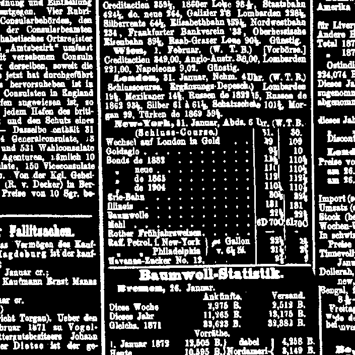
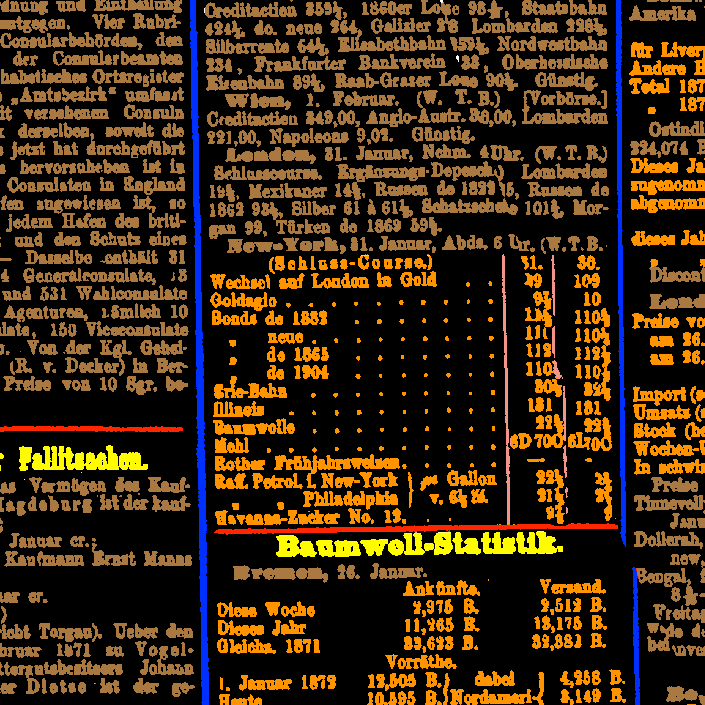
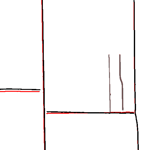
Figure 2: Left: Binarized version of BBZ page. Middle: Manually annotated version before preprocessing (using various label classes that were later combined to the ones given in the previous section). Right: Separator ground truth for warped (black) and unwarped (red) version of the image.

3.3 Postprocessing Ground Truth

The better the quality of the ground truth, the better a DNN can learn to deal with ambiguous situations. For this reason, we performed a number of rule-based normalization procedures on our manual annotations that aimed at generalizing them and removing noise that is inherent in manual, pixel-wise annotation. More concretely, we used rule-based cleanups tuned for our specific corpus. For example, for text and table blocks, we morphologically closed the annotated blocks into solid shapes without connecting adjacent blocks. For separators we detected broken lines and reconnected them, up to a certain threshold. We used heuristic rules to decide whether two blocks which got merged through a morphological closing operation should actually stay merged, based on their respective line heights (the latter were computed by running Tesseract on the polygonal text block’s image). We manually verified all these heuristic operations on our training data.

In the next step, images were scaled down to their intended image size (defined later below as part of our tiling configurations, see Table 3) during training. Since scaling schemes like linear interpolation or nearest neighbor would destroy indexed label information, our scaling approach used an area filter that gave weights to labels and then picked the one label in each source pixel area that had the highest summed weight. By choosing higher weights for separator labels, we ensured that their thin line annotations did not get destroyed or broken during the scaling process.

For data augmentation, we also added slightly warped versions of each image. We modified source images and annotations by identical projections onto a mesh derived from pseudorandom cubic splines. Once again, this operation used special area filters for scaling. We basically reversed the approach described in [18] (see Figure 2 for an illustration). Note that this data augmentation was independent of the later data augmentation during the training.

Both warped and non-warped images were then scaled and/or split into overlapping tiles, as described in section 4.1.7. Since folds were defined over pages (not tiles), so all tiles belonged to either validation or training set, i.e. there was no danger of information leakage between training and validation sets.

4 Training the DNN Model

In this section, we provide a review of existing DNN architectures and explain our choice of an architecture that – given the accompanying ground truth – is capable of learning and predicting our previously described segmentation tasks with the best possible quality.

4.1 Architectures and Hyperparameters

There are many parameters to consider when training a DNN for the specified tasks. In the following sections, we consider some fundamental options and explain how we came up with an optimal configuration that best suits our needs.

4.1.1 Configuration Space

Semantic segmentation networks consist of two architectures: (1) a backbone network that performs the visual recognition tasks and that acts as an encoder, and (2) an overall architecture for the segmentation network as a whole [12], to which we will refer to as s-model (for segmentation model) from here on. For example, ResNet [19] is a well-established recognition backbone used in many real-world U-Net implementations, whereas U-Net [20] is a well-established s-model architecture.

In our search for a specific segmentation DNN (i.e. a network consisting of both a backbone and a s-model), and following the terminology of configuration spaces as described by Feurer and Hutter [21], we defined a configuration space ${\mathbf{\Theta}}$ as

$$\mathbf{\Theta}=\Theta_{s-model}\times\Theta_{backbone}\times\Theta_{tiling}\times\Theta_{optimizer}\times\Theta_{loss}$$ (1)

$\Theta_{optimizer}$ is the optimization algorithm used for training the model, $\Theta_{loss}$ is the DNN’s loss function during training.

4.1.2 Evaluation Metric

There are various measures at hand when it comes to evaluating the pixel-segmentation tasks, among them the well-known F1 score [22], while others are based on pixel accuracy and intersection over union (IOU) [23]. However, it is unclear which of these measures is best suited as an indicator for overall quality in a ranking.. In the context of OCR of historical documents, Wick and Puppe [7] report issues with Long et al.’s proposed metrics and suggest an alternative pixel accuracy metric. At the same time, it is known that pixel accuracy is generally not well suited for imbalanced label classes like our blkx and sep tasks.

From this situation, we decided to evaluate the overall quality of our models using an altogether different metric, namely a multi-class extension of the Matthews Correlation Coefficient (MCC). For binary classification Chicco and Jurman report that ”F1 score and accuracy can mislead, but MCC does not” [25], and note that, in a ranking experiment of various classifier algorithms ”[t]he F1 score ranking and the accuracy ranking, in conclusion, are hiding [an] important flaw of the top classifier” [25]. While we are aware that for pixel segmentation, MCC does not seem to be a widely used metric at the moment, and that other metrics have also been studied and proposed in this context [4, 24, 26], we think the arguments in [25] are very plausible and believe that the MCC is also well-suited for our ranking experiments on highly unbalanced label classes.

4.1.3 Grid Search: General Approach

In order to identify the optimal configuration of hyperparameters, we performed a grid search. For both the grid search as well as the final model we made use of models pretrained on ImageNet [15, 22]. All models were trained on our full training data for 50 epochs with a batchsize of 3 and a learning rate of $2.5\text{\times}{10}^{-3}$. For evaluation we only used fold 1 of an 80-20 split between training data and validation data. Furthermore, we used automatic data augmentation via [27] with (1) rotation of up to $\pm 10$ degrees (applied always) and (2) contrast manipulation with a probability of 90% using default settings.

4.1.4 Choices for $\Theta_{optimizer}$ and $\Theta_{loss}$

In a first step, we pinned $\Theta_{s-model}$ to ResNet-18, $\Theta_{backbone}$ to U-Net, and $\Theta_{tiling}$ to an untiled 896 x 128 scaling, to find good values for $\Theta_{optimizer}$ and $\Theta_{loss}$. For $\Theta_{loss}$, categorical cross-entropy loss proved best for blk and blkx, whereas generalized dice loss [28] showed the best results for sep. For $\Theta_{optimizer}$ we obtained very stable convergence and good results with an Adam optimizer with decoupled weight decay regularization [29], lookahead [30] and cosine annealing. Various other current optimizers we tried showed numerical instabilities with our training data.

In a second step, we pinned $\Theta_{optimizer}$ and $\Theta_{loss}$ and performed a grid search over $\Theta_{s-model}$, $\Theta_{backbone}$ and $\Theta_{tiling}$ (see the following sections).

4.1.5 Choices for $\Theta_{s-model}$

$\Theta_{s-model}$ included U-Net [20] and FPNs [12]. We also evaluated LinkNet [31] and PSPNet in a large prior grid search, but they gave consistently worse results than U-Net and FPN, so for the sake of minimizing the already huge grid evaluation runtimes, we decided to exclude those models from the actual evaluation.

4.1.6 Choices for $\Theta_{backbone}$

Based on [16], our batch size, and GPU memory constraints, we picked the following architectures as representative of all possible choices: VGG16, ResNet-34, ResNet-50, SE-ResNet-34, SE-ResNet-50, SE-ResNeXt-50, Inception-v3, Inception-ResNet-v2. We also included variants of the rather new EfficientNet [32], namely EfficientNet-B1 and EfficientNet-B2, but omitted EfficientNet-B3 and higher since we ran out of GPU memory on our V100 with our standard batch size for them.

Note that in general we restricted ourselves to models that allowed us to carry out at least batch sizes of 3 (due to batch norm and other considerations) on all tile configurations.

4.1.7 Choices for $\Theta_{tiling}$

As document images are generally large (e.g. at least $2,400\times 3,400$ pixels in a medium-sized version of the BBZ) it is not possible to train a model on the entire, unscaled image with current GPUs. One important aspect thus is the scaling size of the images for training and prediction. Accordingly, three questions arise: should we (a) just scale down images (thereby losing information), (b) split images into smaller parts, i.e. into tiles or patches (thereby losing context), or (c) do both.

Unfortunately, in this general form, these three questions are rather intractable. Therefore, we need to generate specific examples that we can test and interpret. We also need to pick specific image resolutions, specific tile patterns (e.g. horizontal vs. vertical), specific GPU hardware and, finally, specific combinations of those factors that will allow us extrapolate answers to the above questions. In other words, we sample a small subset from a very large population of possible combinations and use these as parameters for $\Theta_{tiling}$ in our grid search.

In this manner, we first need to pick specific image resolutions to investigate. To this end, we explored the maximum (technically) possible size of an image or tile on certain GPUs (see below). Based on this maximum size, we then carefully designed a number of tiling configurations that include mixed and border cases that model important features from (a), (b) and (c).

As GPU hardware for all further tests, we picked two GPUs that seem representative of current top-tier and enterprise-grade GPU hardware and therefore are of large practical interest for institutions having one or the other: a NVIDIA GeForce RTX 2080 Ti with 12 GB GPU RAM and a NVIDIA Tesla V100 with 32 GB GPU RAM. We explored RAM limits of those GPUs by empirically searching for resolutions that (i) matched our corpus document image aspect ratio and other side constraints, (ii) were as large as possible, (iii) would allow us to train all models investigated in our grid search using [22] and (iv) use batch size 3. The largest feasible resolutions we found were $512\times 768$ (0.39 megapixels) on the GeForce RTX 2080 Ti, and $896\times 1280$ (1.15 megapixels) on the V100. From here on, we call these two pixel counts, i.e. 1.15M and 0.39M, maximum sizes - as they are the maximum number of pixels trainable on those GPUs. As these are the limits of current GPU hardware, they are of great practical importance and will become pivotal in the following discussion.

                               

Figure 3: Tiling patterns. Left: Horizontal tiling (h). Middle: Vertical tiling (v). Right: Rectangular tiling (h, v). Note that tiles have been slightly shifted for better illustration. All tiles exhibit overlap. During inference, tiles are merged halfway at their overlaps.

We now reframe our very general questions (a), (b) and (c) into two tractable research questions (1) and (2) that can be evaluated on our specific GPU hardware:

(1) Fix Total Size, Vary Tile Size.. Looking at a document image with a pixel count $N$, we ask ourselves, what is the difference between processing it as a whole vs. tiling it using h, v or hv patterns (see Figure 3)? In other words, what decrease in quality should we expect with tiled configurations of a fixed overall image resolution as opposed to processing the image as a whole?

(2) Fix Tile Size, Vary Total Size. Again, assuming some number of pixels $N$, we ask: what is the best use we can put these pixels to, i.e. should we train on a downscaled image of maximum size as a whole or should we use a bigger image (that does not fit on the GPU) and use tiles of maximum size?

While we could have evaluated (1) and (2) for many pixel counts $N$ and on both GPUs, because of the huge runtimes involved and to minimize GPU computation time, we chose to evaluate (1) only for $N=1.15M$ (i.e. the maximum size of the V100 case), and (2) partially (namely for -, h, v) for $N=0.39M$ (i.e. the maximum size of the GeForce RTX 1080 Ti case), and partially (namely for v and hv) for $N=1.15M$.

configuration	total size	tile size	tiling
GeForce RTX 2080 Ti
{34cm[ fixed tile size ] $0.3/-$	$max$	$max$	-
$0.6/h$	$>max$	$max$	h
$0.9/v$	$>max$	$max$	v
V100
{44cm[ fixed total size ] $1.1/-$	$max$	$max$	-
$1.1/h$	$max$	$<max$	h
$1.1/v$	$max$	$<max$	v
$1.1/hv$	$max$	$<max$	hv
{24cm[ fixed tile size ] $3.0/v$	$>max$	$max$	v
$3.9/hv$	$>max$	$max$	hv

Table 2: Tiling configurations and related research questions, grouped by GPUs. $max$ indicates the maximum number of pixels for the respective GPU. For tiling patterns referenced here, see Figure 3. As described in the text, configuration names consist of a prefix (e.g. $1.1$) indicating overall total size as pixel count followed by a tile pattern.

name	total size			tiling		tile size
	resolution	#pixels		pattern	#tiles	resolution	#pixels
$0.3/-$	$512\times 768$	0.39M		$-$	$-$	$-$	$-$
$0.6/h$	$640\times 1024$	0.66M		h	2	$384\times 1024$	0.39M
$0.9/v$	$768\times 1280$	0.98M		v	3	$768\times 512$	0.39M
$1.1/h$	$896\times 1280$	1.15M		h	5	$256\times 1280$	0.33M
$1.1/v$	$896\times 1280$	1.15M		v	4	$896\times 384$	0.25M
$1.1/hv$	$896\times 1280$	1.15M		h, v	4	$512\times 768$	0.39M
$1.1/-$	$896\times 1280$	1.15M		$-$	$-$	$-$	$-$
$3.0/v$	$1280\times 2400$	3.07M		v	3	$1280\times 896$	1.15M
$3.9/hv$	$1640\times 2400$	3.94M		h, v	4	$896\times 1280$	1.15M

Table 3: Details of the Tiling configurations. Maximum sizes are printed in bold.

Table 2 gives a concise overview of the main ideas just described. Table 3 gives more detailed information on the resolutions used. In both tables we use a naming scheme for tile configurations that consists of a prefix indicating the overall size of the scaled, untiled document (e.g., by definition, $1.15$ for a total size of 1.15 megapixels) followed by the kind of tiling applied on it (e.g. $/h$ indicating some kind of horizontal tiling). This notation is clearly inexact, as it does not specify the tile size, and is therefore only intended as a shorthand for the more detailed data in Tables 2 and 3.

As illustration of the notation, three specific scenarios from question (2) are as follows: (2a) use all pixels in one image without tiling ($0.39/-$), (2b) use a bigger sized image and use all available pixels for horizontal tiles ($0.66/h$), (2c) use an even bigger sized image and use available pixels for vertical tiles ($0.98/v$).

4.1.8 Results of Grid Search

The results of our grid search over the described configuration space are given in Table 4. Without preliminary studies and without dhSegment (which we evaluated separately), we evaluated $9\times 10\times 3\times 2$ (each configuration, each backbone, three tasks, for both U-Net and FPN) $=540$ data points. On average, each data point took about 15 hours of GPU time to compute.

configuration	$0.3/-$	$0.6/h$	$0.9/v$	$1.1/h$	$1.1/v$	$1.1/hv$	$1.1/-$	$3.0/v$	$3.9/hv$
results for sep:
VGG16	91.29	91.67	91.51	82.74	90.77	90.58	90.59	90.87	89.52
ResNet-34	89.45	90.60	90.85	82.46	90.54	90.34	90.24	90.72	89.82
ResNet-50	89.93	90.94	91.43	82.61	90.22	90.41	90.45	90.79	89.63
SE-ResNet-34	89.91	91.17	91.12	82.57	90.32	90.57	90.18	91.19	89.82
SE-ResNet-50	90.73	91.32	91.70	82.95	90.34	90.75	90.69	91.44	89.92
SE-ResNeXt-50	90.77	91.45	91.62	82.97	90.88	90.81	90.03	91.24	90.05
EfficientNet-B1	91.36	92.01	91.84	83.17	91.09	91.08	91.18	91.64	90.21
EfficientNet-B2	91.63	91.70	91.86	83.34	91.04	91.15	91.07	91.70	90.27
Inception-v3	91.06	91.42	91.19	82.80	90.69	90.96	89.99	91.21	89.84
Inception-ResNet-v2	91.18	91.64	91.41	82.92	90.70	90.85	90.94	91.09	89.96
dhSegment	65.24	80.42	77.57	80.79	75.92	74.91	69.69	73.47	83.52
results for blk:
VGG16	92.01	93.06	93.81	91.21	94.07	93.84	93.24	94.68	93.82
ResNet-34	93.56	93.59	94.20	91.97	94.27	94.00	94.33	95.00	94.50
ResNet-50	93.21	93.39	94.58	91.58	94.60	94.06	94.79	95.04	94.45
SE-ResNet-34	92.49	93.50	93.85	91.49	94.39	94.22	94.10	95.16	94.42
SE-ResNet-50	93.53	93.85	94.59	91.82	94.79	94.60	94.39	94.86	94.61
SE-ResNeXt-50	93.61	93.88	94.93	92.19	94.69	94.65	94.73	95.05	94.61
EfficientNet-B1	92.83	93.38	94.17	91.63	94.23	94.05	93.74	94.96	94.56
EfficientNet-B2	92.59	93.07	94.11	91.81	94.18	94.07	94.19	95.03	94.59
Inception-v3	93.15	93.25	93.70	91.59	94.52	94.24	94.53	95.30	94.76
Inception-ResNet-v2	94.14	93.98	94.85	91.64	95.01	94.47	95.07	95.79	95.32
dhSegment	92.95	94.03	94.48	94.09	94.47	94.17	93.41	94.37	94.36
results for blkx:
VGG16	91.50	93.32	93.61	91.03	93.44	93.37	93.23	93.94	93.21
ResNet-34	92.70	93.09	93.57	91.15	94.11	93.33	93.54	94.65	93.73
ResNet-50	92.42	93.28	94.03	91.29	94.17	93.66	93.80	94.59	93.81
SE-ResNet-34	92.59	92.83	94.08	91.43	93.93	93.62	93.68	94.60	94.41
SE-ResNet-50	92.60	93.70	94.11	91.65	94.30	93.90	94.27	94.67	94.14
SE-ResNeXt-50	93.37	93.80	94.19	91.59	94.16	94.36	94.29	94.52	93.95
EfficientNet-B1	92.32	92.96	94.02	90.90	93.65	93.77	93.60	94.61	94.28
EfficientNet-B2	92.26	93.11	93.65	91.35	93.82	93.60	93.87	94.85	94.27
Inception-v3	92.99	93.38	94.01	91.50	94.02	93.88	93.99	95.08	94.34
Inception-ResNet-v2	93.32	93.73	94.78	91.71	94.65	94.58	94.60	95.51	94.91
dhSegment	92.91	94.19	94.44	94.04	94.29	94.03	93.26	94.35	94.25

Table 4: Matthew correlation coefficients (MCCs) all evaluated models in grid search. Column titles are the tile configuration names described in Table 3. Shown results include $\Theta_{s-model}$ with both U-Net and FPN (only best variant is shown). Best values in each column are bold (per task).

The actual numbers make a simple comparison difficult, since they are relative to resolution. Seeing a similar number between a smaller resolution or tile size and a larger resolution does not indicate that the result on the larger resolution is worse, it might in fact be even better. On the other hand, a higher number on a higher resolution configuration (i.e. a more difficult problem) should always indicate a better result.

With these caveats in mind, here are some observations on this data:

Tasks. In general, blk yields better results (higher scores) than blkx, which is expected, as blk is a simpler task. See Figure 4 for how much better the results are for blk.

Backbone Architecture. For the sep task, EfficientNet outperforms all other architectures..

For blk, blkx we see three notable architectures: SE-ResNeXt-50, Inception-ResNet-v2, and dhSegment. The latter performs better (but not great) on h tilings than the other architectures, which might itself be an artefact due to dhSegment’s internal scaling. In general, Inception-ResNet-v2 (which is in fact the best backbone architecture among the tested ones [16]) seems to outperform all other architectures as the complexity of task gets harder (going from blk to blkx), or as the resolution of the image gets higher. We also observe that more powerful backbone architectures seem to expose a less severe drop of performance when going from blk to blkx (see Figure 4).

Figure 4: Left: Minimum, maximum and mean MCC (over all tiling configurations) for several backbones (color coded by family, e.g. Inception is green) regarding blk (thin lines, left) and blkx (thick lines, right). Sorted from lowest absolute mean decrease when going from blk to blkx (left) to largest decrease (right). Right: Quality of trained models vs. number of training pages used (using a constant test set). This analysis was done on configuration $3.0/v$ with Inception-ResNet-v2.

S-Model Architectures. We investigated both FPN and U-Net, but did not find systematic or large performance differences between the two. That said, our final models (based on $3.0/v$) achieved their best scores on all three tasks with FPN.

Tiling and Resolution. We find that higher resolutions generally seems to improve results, but observe a strong dependency on the mode of tiling used on how big that gain actually is, with v tiling showing the highest relative increase per resolution increase (see left plot in Figure 5). Notably, this general observation does not hold true for h tiling and for VGG16. The latter is the only tested model that decreases performance for the hv and even the untiled mode with increased resolution and shows no clear increase for v (see right plot in Figure 5).

Figure 5: Left: Solid areas of best (solid lines) and worst (dotted lines) performance of all blkx models in our grid search (without VGG16). Except for h, performance increases as overall image resolution increases, most notably for untiled and for v. Right: Performance of backbone VGG16, which bucks the general trend and tends to get worse as image resolution increases.

Our research questions concerning tiling can be answered as follows:

(1) when fixing total size while varying tile size, we see different results for different tasks. For sep and blkx, tile patterns v, hv and ”no tiling” are close, whereas h tiling is clearly worse (see $1.1$, $1.1/h$, $1.1/v$, $1.1/hv$). For blk, on the other hand, only v-tiling is close to the untiled version.

(2) when fixing tile size while varying total size, vertical tiles seem to work best for blk and blkx (see $0.9/v$ vs. $0.3/-$ and $0.6/h$). For sep, on the other hand, this does not seem true, as indeed $0.6/h$ performs best for various backbones.

Still, taking into account all tasks and the bad results for $1.1/h$, we argue that v-tiling seems to be the best general option for training newspaper data sets, as it yields results that are consistently close to untiled training across various tasks.

Partial Data. Additional experiments with using only parts of our training data indicate that a training data set of 20 to 40 pages already gives very good results (see Figure 4). More specifically, we already see $99\%$ of the performance of our full (84 page) training set at 24 pages for blkx and at 41 pages for sep. Thus, for blkx, tripling the amount of training data from 24 pages to 72 pages only yields a relative gain in MCC of less than $1\%$.

4.2 Final Model

In Table 5, we show results for our final models. We also reprint the results from [8] to illustrate that our approach seems to work reasonably well in its domain. Note that [7] also report a pixel accuracy of 98.4% on St. Gall. Inference for one fold takes about $0.63s$ per page on the V100. Following our reliance on MCC, we pick sep/fold2 (and not sep/fold4) as best fold for sep.

task	fold	pixel accuracy	mean acc.	mean IU	f.w. IU	MCC
sep	1	99.76	87.06	81.24	99.58	91.51
sep	2	99.77	89.58	85.03	99.58	92.08
sep	3	99.72	85.83	79.61	99.52	89.85
sep	4	99.79	86.90	81.50	99.62	91.39
sep	5	99.73	89.48	83.49	99.51	90.24
blkx	1	97.58	77.16	74.86	95.52	95.76
blkx	2	97.96	88.77	85.88	96.10	96.14
blkx	3	97.68	89.22	86.30	95.63	95.86
blkx	4	98.86	94.53	92.67	97.82	97.83
blkx	5	98.17	88.55	85.86	96.78	96.35
G. Washington [8]		91	91	77	86	-
Parzival [8]		94	75	68	89	-
St. Gall [8]		98	90	87	96	-

Table 5: Final $3.0/v$ models and reference scores from [8]. Best scores in each columns (and for each task) are bold.

5 Conclusion

We were able to re-support the claim that pixel-by-pixel segmentation approaches can be applied very successfully to newspapers, and furthermore showed that transfer learning works well in this context. We also showed that detection of table areas and separators works reasonably well for even complex layouts. Furthermore, we investigated the influence of various factors, such as tiling configurations or the influence of number of labels (i.e. blk vs blkx) and found data supporting the idea that vertical tilings work well. Finally, we showed that a training data set of 30 to 40 pages already gives reasonably good results.

Our study is intended to be a starting point for further research with more carefully chosen tile and resolution subsets. We hope our data can offer valuable guidelines for groups working on similar problems.

Appendix

Figure 6: Examples from blkx/fold-4. Left: Scanned page. Middle: Ground truth. Right: Prediction.

Figure 7: Examples from sep/fold-2. Text separators show as green lines, table column separators as blue lines. Left: Scanned page. Middle: Ground truth. Right: Prediction.

References

- [1] S. Graham, I. Milligan, and S. Weingart. Exploring Big Historical Data: The Historian’s Macroscope. Imperial College Press, 2015.
- [2] Faisal Shafait. Geometric layout analysis of scanned documents. Dissertation, Technical University of Kaiserslautern, 2008.
- [3] Amy Winder. Extending the Page Segmentation Algorithms of the OCRopus Documentation Layout Analysis System. PhD thesis, Boise State University, 2010.
- [4] Martin Thoma. A survey of semantic segmentation. CoRR, abs/1602.06541, 2016.
- [5] F. Shafait, D. Keysers, and T. Breuel. Performance evaluation and benchmarking of six-page segmentation algorithms. IEEE Transactions on Pattern Analysis and Machine Intelligence, 30(6):941–954, 2008.
- [6] Sofia Ares Oliveira, Benoit Seguin, and Frédéric Kaplan. dhsegment: A generic deep-learning approach for document segmentation. CoRR, abs/1804.10371, 2018.
- [7] Christoph Wick and Frank Puppe. Fully convolutional neural networks for page segmentation of historical document images. CoRR, abs/1711.07695, 2017.
- [8] Kai Chen and Mathias Seuret. Convolutional neural networks for page segmentation of historical document images. CoRR, abs/1704.01474, 2017.
- [9] Benjamin Bruno Meier, Thilo Stadelmann, Jan Stampfli, Marek Arnold, and Mark Cieliebak. Fully convolutional neural networks for newspaper article segmentation. In ICDAR, pages 414–419. IEEE, 2017.
- [10] Lorenzo Quirós. P2pala: Page to page layout analysis tookit. https://github.com/lquirosd/P2PaLA, 2017. GitHub repository.
- [11] Kaiming He, Georgia Gkioxari, Piotr Dollár, and Ross B. Girshick. Mask R-CNN. CoRR, abs/1703.06870, 2017.
- [12] Xiaolong Liu, Zhidong Deng, and Yuhan Yang. Recent progress in semantic image segmentation. CoRR, abs/1809.10198, 2018.
- [13] Asifullah Khan, Anabia Sohail, Umme Zahoora, and Aqsa Saeed Qureshi. A survey of the recent architectures of deep convolutional neural networks. CoRR, abs/1901.06032, 2019.
- [14] Jason Yosinski, Jeff Clune, Yoshua Bengio, and Hod Lipson. How transferable are features in deep neural networks? In Z. Ghahramani, M. Welling, C. Cortes, N. D. Lawrence, and K. Q. Weinberger, editors, Advances in Neural Information Processing Systems 27, pages 3320–3328. Curran Associates, Inc., 2014.
- [15] Olga Russakovsky, Jia Deng, Hao Su, Jonathan Krause, Sanjeev Satheesh, Sean Ma, Zhiheng Huang, Andrej Karpathy, Aditya Khosla, Michael S. Bernstein, Alexander C. Berg, and Fei-Fei Li. Imagenet large scale visual recognition challenge. CoRR, abs/1409.0575, 2014.
- [16] Simone Bianco, Rémi Cadène, Luigi Celona, and Paolo Napoletano. Benchmark analysis of representative deep neural network architectures. CoRR, abs/1810.00736, 2018.
- [17] Muhammad Zeshan Afzal, Martin Krämer, Syed Saqib Bukhari, Mohammad Reza Yousefi, Faisal Shafait, and Thomas M. Breuel. Robust binarization of stereo and monocular document images using percentile filter. In Masakazu Iwamura and Faisal Shafait, editors, CBDAR, volume 8357 of Lecture Notes in Computer Science, pages 139–149. Springer, 2013.
- [18] Matt Zucker. Page dewarping. https://mzucker.github.io/2016/08/15/page-dewarping.html, 2016.
- [19] Kaiming He, Xiangyu Zhang, Shaoqing Ren, and Jian Sun. Deep residual learning for image recognition. CoRR, abs/1512.03385, 2015.
- [20] Olaf Ronneberger, Philipp Fischer, and Thomas Brox. U-net: Convolutional networks for biomedical image segmentation. CoRR, abs/1505.04597, 2015.
- [21] Matthias Feurer and Frank Hutter. Hyperparameter optimization. In Frank Hutter, Lars Kotthoff, and Joaquin Vanschoren, editors, AutoML: Methods, Sytems, Challenges, chapter 1, pages 3–33. Springer, May 2019.
- [22] Pavel Yakubovskiy. Segmentation models. https://github.com/qubvel/segmentation_models, 2019. GitHub repository.
- [23] Evan Shelhamer, Jonathan Long, and Trevor Darrell. Fully convolutional networks for semantic segmentation. CoRR, abs/1605.06211, 2016.
- [24] Eduardo Fernández-Moral, Renato Martins, Denis Fernando Wolf, and Patrick Rives. A new metric for evaluating semantic segmentation: Leveraging global and contour accuracy. 2018 IEEE Intelligent Vehicles Symposium (IV), pages 1051–1056, 2018.
- [25] Davide Chicco and Giuseppe Jurman. The advantages of the matthews correlation coefficient (mcc) over f1 score and accuracy in binary classification evaluation. BMC Genomics, 21, 12 2020.
- [26] Gabriela Csurka and Diane Larlus. What is a good evaluation measure for semantic segmentation? In Tilo Burghardt, Dima Damen, Walterio W. Mayol-Cuevas, and Majid Mirmehdi, editors, British Machine Vision Conference, BMVC 2013, Bristol, UK, September 9-13, 2013, volume 26. BMVA Press, 01 2013.
- [27] Alexander V. Buslaev, Alex Parinov, Eugene Khvedchenya, Vladimir I. Iglovikov, and Alexandr A. Kalinin. Albumentations: fast and flexible image augmentations. CoRR, abs/1809.06839, 2018.
- [28] Carole H. Sudre, Wenqi Li, Tom Vercauteren, Sébastien Ourselin, and M. Jorge Cardoso. Generalised dice overlap as a deep learning loss function for highly unbalanced segmentations. CoRR, abs/1707.03237, 2017.
- [29] Ilya Loshchilov and Frank Hutter. Fixing weight decay regularization in adam. CoRR, abs/1711.05101, 2017.
- [30] Michael R. Zhang, James Lucas, Geoffrey E. Hinton, and Jimmy Ba. Lookahead optimizer: k steps forward, 1 step back. CoRR, abs/1907.08610, 2019.
- [31] Abhishek Chaurasia and Eugenio Culurciello. Linknet: Exploiting encoder representations for efficient semantic segmentation. CoRR, abs/1707.03718, 2017.
- [32] Mingxing Tan and Quoc V. Le. Efficientnet: Rethinking model scaling for convolutional neural networks. CoRR, abs/1905.11946, 2019.