Astronomy Letters, 2020, Vol. 46, No 2, pp. 131–143.

Kinematics of T Tauri Stars Close to the Sun from

the Gaia DR2 Catalogue

V.V. Bobylev

Pulkovo Astronomical Observatory, Russian Academy of Sciences,

Pulkovskoe sh. 65, St. Petersburg, 196140 Russia

Abstract—The spatial and kinematic properties of a large sample of young T Tauri stars from the solar neighborhood 500 pc in radius have been studied. The following parameters of the position ellipsoid have been determined from the most probable members of the Gould Belt: its sizes are $350\times 270\times 87$ pc and it is oriented at an angle of $14\pm 1^{\circ}$ to the Galactic plane with a longitude of the ascending node of $297\pm 1^{\circ}$. An analysis of the motions of stars from this sample has shown that the residual velocity ellipsoid with principal semiaxes $\sigma_{1,2,3}=(8.87,5.58,3.03)\pm(0.10,0.20,0.04)$ km s^-1 is oriented at an angle of $22\pm 1^{\circ}$ to the Galactic plane with a longitude of the ascending node of $298\pm 2^{\circ}$. It has been established that much of the expansion effect (kinematic $K$ effect) typical for Gould Belt stars, 5–6 km s^-1 kpc^-1, can be explained by the influence of a Galactic spiral density wave with a radial perturbation amplitude $f_{R}\sim 5$ km s^-1.

INTRODUCTION

The Gould Belt is a fairly flat system with semiaxes of $\sim 350\times 250\times 50$ pc, with the direction of its semimajor axis being near $l=40^{\circ}$ (Efremov 1989; Pöppel 1997, 2001; Torra et al. 2000; Olano 2001). The plane of its symmetry is inclined to the Galactic plane approximately at $i=18^{\circ}$. The longitude of the ascending node is $l_{\Omega}=280^{\circ}$. The Sun is at a distance of $\sim 40$ pc from the line of nodes. The system’s center lies at a heliocentric distance of 100–150 pc in the second Galactic quadrant. The estimate of the direction to the center $l_{0}$ depends on the sample age and, according to various published sources, ranges from $130^{\circ}$ to $180^{\circ}$. The spatial distribution of stars is highly nonuniform—a noticeable drop in density is observed within $\approx 80$ pc of the center, i.e., the entire system has the shape of a doughnut. The well-known open star cluster $\alpha$ Per with an age of $\sim 35$ Myr lies near the center of this doughnut. A number of nearby OB associations (de Zeeuw et al. 1999) and open star clusters (Piskunov et al. 2006; Bobylev 2006), dust (Dame et al. 2001; Gontcharov 2019) and molecular (Perrot and Grenier 2003; Bobylev 2016) clouds belong to the Gould Belt; a giant neutral hydrogen cloud called the Lindblad ring (Lindblad 1967, 2000) is associated with it.

We know about the kinematic properties of the Gould Belt from an analysis of the motions of young massive O- and B-type stars (Torra et al. 2000), young open star clusters (Piskunov et al. 2006; Bobylev 2006; Vasilkova 2014), and molecular clouds (Perrot and Grenier 2003; Bobylev 2016). In particular, evidence of expansion and intrinsic rotation of this system has been found. Using the Scorpius–Centaurus association closest to the Sun (on a scale of $\sim 150$ pc) as an example, Sartori et al. (2003) showed the absence of differences in distribution and kinematics between massive and low-mass (T Tauri) stars of comparable age. On a larger scale ($\sim 1$ kpc in diameter) a kinematic analysis of T Tauri stars has not yet been performed due to the absence of necessary measurements. With the appearance of the Gaia DR2 catalogue (Brown et al. 2018; Lindegren et al. 2018), it has become possible to select tens of thousands of such stars (Zari et al. 2018) that belong to known associations closely related to the Gould Belt. These include the Scorpius–Centaurus, Orion, Vela, Taurus, Cepheus, Cassiopeia, and Lacerta associations.

An expansion of individual OB associations (Blaauw 1964), groupings of young associations close to the Sun (Torres et al. 2008), samples of young massive OB stars (Torra et al. 2000), and a large complex of young open star clusters (Piskunov et al. 2006; Bobylev 2006) has been noticed in the Gould Belt region. There is no certainty in the question of what center or line the expansion originates from, because the effect manifests itself as a dependence of the velocities $U$ and $V$ on coordinates $x$ and $y.$ Bobylev (2014) suggested that much of the Gould Belt expansion could be explained by the influence of a spiral density wave. A practical allowance for the effect, apparently, has not yet been made and, therefore, the results of this approach are of great interest.

The goal of this paper is to determine the spatial and kinematic properties of a large sample of T Tauri stars from the Gaia DR2 catalogue selected by Zari et al. (2018). Such an analysis suggests a study of the system’s spatial orientation, a confirmation of the system’s expansion and intrinsic rotation typical for the Gould Belt, and an analysis of the residual stellar velocities.

DATA

In this paper we use the compilation by Zari et al. (2018) that contains more than 40 000 T Tauri stars selected from the Gaia DR2 catalogue by kinematic and photometric data. These stars are within 500 pc of the Sun, because the restriction on the sample radius $\pi>2$ milliarcseconds (mas) was used. They were selected by proper motions through an analysis of the smoothed distribution of points on the $\mu_{\alpha}\cos\delta\times\mu_{\delta}$ plane using the restriction on the tangential stellar velocity $\sqrt{\mu^{2}_{\alpha}\cos\delta+\mu^{2}_{\delta}}<40$ km s^-1.

The following three subsamples of T Tauri stars are presented in the catalogue by Zari et al. (2018):

(i) PMS1 that includes 43 719 stars within the outermost contour constructed when smoothing the points on the $\mu_{\alpha}\cos\delta\times\mu_{\delta},$ plane and, therefore, this sample contains the largest number (compared to the two remaining ones) of background objects;

(ii) PMS2 that contains 33 985 stars within the second contour on the $\mu_{\alpha}\cos\delta\times\mu_{\delta},$ plane;

(iii) PMS3 that contains 23 686 stars within the third contour and, therefore, they are the most probable members of the kinematic grouping (Gould Belt).

In addition, there is a sample of early-type stars from the Gaia DR2 catalogue located in the upper main sequence on the Hertzsprung–Russell (H–R) diagram designated as UMS. It contains 86 102 stars with an absolute magnitude $M_{G,0}$ less than 3.5${}^{m}.$ In the opinion of Zari et al. (2018), this sample includes stars of spectral types O, B, and A.

The line-of-sight velocities in the catalogue by Zari et al. (2018) were taken from various sources, in particular, from the Gaia DR2 catalogue. However, the stars with line-of-sight velocities are much fewer than the stars with proper motions. Figure 1 presents the H–R diagram constructed from the stars of the UMS and PMS3 samples. On this diagram the stars with measured line-of-sight velocities are marked; the stars with line-of-sight velocity measurement errors no more than 5 km s^-1 were taken. It can be seen that there are few very young stars and stars with measured line-of-sight velocities in the UMS sample, while in the PMS3 sample, on the contrary, the stars with measured line-of-sight velocities are relatively more luminous and evolutionally most advanced, because they are close to the main sequence on the H–R diagram.

As shown by Zari et al. (2018), the stars of all the samples presented by them, PMS1, PMS2, PMS3, and, to a lesser degree, UMS, have a close spatial association with the Gould Belt.

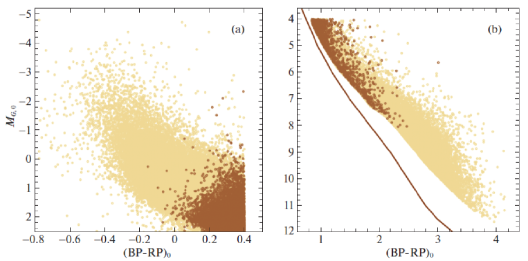
Figure 1: (Color online) The H–R diagram constructed from the UMS (a) and PMS3 (b) stars, the dark circles mark the stars with measured line-of-sight velocities, the solid line marks the main sequence.

METHODS

We use a rectangular coordinate system centered on the Sun in which the $x$ axis is directed toward the Galactic center, the $y$ axis is in the direction of Galactic rotation, and the $z$ axis is directed toward the north Galactic pole. Then, $x=r\cos l\cos b,$ $y=r\sin l\cos b$ and $z=r\sin b.$

We know three stellar velocity components from observations: the line-of-sight velocity $V_{r}$ and two tangential velocity components,$V_{l}=4.74r\mu_{l}\cos b$ and $V_{b}=4.74r\mu_{b},$ directed along the Galactic longitude $l$ and latitude $b,$ respectively, expressed in km s^-1. Here, the coefficient 4.74 is the ratio of the number of kilometers in an astronomical unit to the number of seconds in a tropical year and $r=1/\pi$ is the stellar heliocentric distance in kpc that we calculate via the stellar parallax $\pi$ in mas. The proper motion components $\mu_{l}\cos b$ and $\mu_{b}$ are expressed in mas yr^-1.

For each star the velocities $U,V,$ and $W$ can be calculated via the components $V_{r},V_{l},$ and $V_{b},$ where $U$ is directed from the Sun toward the Galactic center, $V$ is in the direction of Galactic rotation, and $W$ is directed to the north Galactic pole:

$$\begin{array}[]{lll}U=V_{r}\cos l\cos b-V_{l}\sin l-V_{b}\cos l\sin b,\\ V=V_{r}\sin l\cos b+V_{l}\cos l-V_{b}\sin l\sin b,\\ W=V_{r}\sin b+V_{b}\cos b.\end{array}$$ (1)

These velocities can be determined only for those stars for which both line-of-sight velocities and proper motions have been measured.

Let us estimate what stellar line-of-sight velocity errors must be in our sample for them to be comparable to the tangential velocity errors. In the Gaia DR2 catalogue the mean parallax errors for bright stars $(G<15^{m})$ lie within the range 0.02–0.04 mas, while for faint stars $(G=20^{m})$ they reach 0.7 mas. Similarly, the proper motion errors range from 0.05 mas yr^-1 for bright stars $(G<15^{m})$ to 1.2 mas yr^-1 for faint ones $(G=20^{m}).$ If we take a proper motion error of 0.1 mas yr^-1, then the tangential velocity error at a sample boundary of 0.5 kpc will be $4.74\times 0.5\times 0.1=0.2$ km s^-1, while for the extreme case, for a proper motion error of 1 mas yr^-1, the tangential velocity error at the sample boundary will be $4.74\times 0.5\times 1=2.4$ km s^-1. Thus, it is desirable to use the stellar line-of-sight velocities with their random measurement errors less than 2.4 km s^-1.

Residual Velocity Formation

When forming the residual velocities, we take into account primarily the peculiar solar velocity, $U_{\odot},$ $V_{\odot}$ and $W_{\odot}$. Since the diameter of the solar neighborhood considered by us is 1 kpc, the influence of the differential Galactic rotation should also be taken into account. Finally, it is interesting to take into account the influence of the Galactic spiral density wave. The expressions for a full allowance for the listed effects are

$$\begin{array}[]{lll}V_{r}=V^{*}_{r}-[-U_{\odot}\cos b\cos l-V_{\odot}\cos b\sin l-W_{\odot}\sin b\\ +R_{0}(R-R_{0})\sin l\cos b\Omega^{\prime}_{0}+0.5R_{0}(R-R_{0})^{2}\sin l\cos b\Omega^{\prime\prime}_{0}\\ +\tilde{v}_{\theta}\sin(l+\theta)\cos b-\tilde{v}_{R}\cos(l+\theta)\cos b],\end{array}$$ (2)

$$\begin{array}[]{lll}V_{l}=V^{*}_{l}-[U_{\odot}\sin l-V_{\odot}\cos l-r\Omega_{0}\cos b\\ +(R-R_{0})(R_{0}\cos l-r\cos b)\Omega^{\prime}_{0}+0.5(R-R_{0})^{2}(R_{0}\cos l-r\cos b)\Omega^{\prime\prime}_{0}\\ +\tilde{v}_{\theta}\cos(l+\theta)+\tilde{v}_{R}\sin(l+\theta)],\end{array}$$ (3)

$$\begin{array}[]{lll}V_{b}=V^{*}_{b}-[U_{\odot}\cos l\sin b+V_{\odot}\sin l\sin b-W_{\odot}\cos b\\ -R_{0}(R-R_{0})\sin l\sin b\Omega^{\prime}_{0}-0.5R_{0}(R-R_{0})^{2}\sin l\sin b\Omega^{\prime\prime}_{0}\\ -\tilde{v}_{\theta}\sin(l+\theta)\sin b+\tilde{v}_{R}\cos(l+\theta)\sin b],\end{array}$$ (4)

where $V^{*}_{r},V^{*}_{l},V^{*}_{b}$ on the right-hand sides of the equations are the original, uncorrected velocities, while $V_{r},V_{l},$ and $V_{b}$ on the left-hand sides are the corrected velocities with which we can calculate the residual velocities $U,V,$ and $W$ based on relations (1), $R$ is the distance from the star to the Galactic rotation axis, $R^{2}=r^{2}\cos^{2}b-2R_{0}r\cos b\cos l+R^{2}_{0}.$ The distance $R_{0}$ is assumed to be $8.0\pm 0.15$ kpc. We take the specific values of the peculiar solar velocity, $(U_{\odot},V_{\odot},W_{\odot})=(11.1,12.2,7.3)$ km s^-1, according to the definition by Schönrich et al. (2010). We use the following kinematic parameters: $\Omega_{0}=28.71\pm 0.22$ km s^-1 kpc^-1, $\Omega^{\prime}_{0}=-4.100\pm 0.058$ km s^-1 kpc^-2, and $\Omega^{\prime\prime}_{0}=0.736\pm 0.033$ km s^-1 kpc^-3, where $\Omega_{0}$ is the angular velocity of Galactic rotation at the distance $R_{0},$ the parameters $\Omega^{\prime}_{0}$ and $\Omega^{\prime\prime}_{0}$ are the corresponding derivatives of this angular velocity. These parameters were determined by analyzing a sample of young open star clusters with the proper motions, parallaxes, and line-of-sight velocities calculated from Gaia DR2 data (see Bobylev and Bajkova 2019a).

We can find two velocities, $V_{R}$ directed radially away from the Galactic center and the velocity $V_{\theta}$ orthogonal to it in the direction of Galactic rotation, based on the following relations:

$$\begin{array}[]{lll}V_{\theta}=U\sin\theta+(V_{0}+V)\cos\theta,\\ V_{R}=-U\cos\theta+(V_{0}+V)\sin\theta,\end{array}$$ (5)

where the position angle $\theta$ satisfies the relation $\tan\theta=y/(R_{0}-x);$ $x,y,$ and $z$ are the rectangular heliocentric coordinates of the star (the velocities $U,V,$ and $W$ are directed along the corresponding $x,y,$ and $z$ axes); and $V_{0}$ is the linear Galactic rotation velocity at the solar distance $R_{0}.$

Here, to take into account the influence of the spiral density wave, we use the simplest model based on the linear theory of density waves by Lin and Shu (1964), in which the potential perturbation is in the form of a traveling wave. Then,

$$\begin{array}[]{lll}\tilde{v}_{R}=f_{R}\cos\chi,\qquad\tilde{v}_{\theta}=f_{\theta}\sin\chi,\qquad\chi=m[{\rm\cot}(i)\ln(R/R_{0})-\theta]+\chi_{\odot},\end{array}$$ (6)

where $f_{R}$ and $f_{\theta}$ are the amplitudes of the radial (directed toward the Galactic center in the arm) and azimuthal (directed along the Galactic rotation) velocity perturbations; $i$ is the spiral pitch angle ($i<0$ for winding spirals); $m$ is the number of arms; $\chi_{\odot}$ is the phase angle of the Sun, in this paper we measure it from the center of the Carina–Sagittarius arm; $\lambda,$ the distance (along the Galactocentric radial direction) between adjacent segments of the spiral arms in the solar neighborhood (the wavelength of the spiral density wave), is calculated from the relation

$${\rm\tan}(i)=\lambda m/(2\pi R_{0}).$$ (7)

The presented method of allowance for the influence of the spiral density wave was used, for example, by Mishurov and Zenina (1999) or Fernández et al. (2001), where its detailed description can be found.

It can be seen that in a small solar neighborhood, as in our case, the position angle $\theta\rightarrow 0^{\circ}$ in Eq. (6) and, therefore, allowance for the spiral density wave does not depend on m. According to the analysis of various stellar samples (Dambis et al. 2015; Rastorguev et al. 2017; Bobylev and Bajkova 2019a; Loktin and Popova 2019), in this paper we adopt the following parameters of the spiral density wave: $\lambda=2.2$ kpc, $f_{R}=5$ km s^-1, $f_{\theta}=0$ km s^-1, and $\chi_{\odot}=-120^{\circ}.$

Residual Velocity Ellipsoid

To determine the parameters of the stellar residual velocity ellipsoid, we use the following well-known method (Trumpler and Weaver 1953; Ogorodnikov 1965). In the classical case, six second-order moments $a,b,c,f,e,$ and $d$ are considered:

$$\begin{array}[]{lll}a=\langle U^{2}\rangle-\langle U^{2}_{\odot}\rangle,\qquad\quad b=\langle V^{2}\rangle-\langle V^{2}_{\odot}\rangle,\qquad\quad c=\langle W^{2}\rangle-\langle W^{2}_{\odot}\rangle,\\ f=\langle VW\rangle-\langle V_{\odot}W_{\odot}\rangle,\quad e=\langle WU\rangle-\langle W_{\odot}U_{\odot}\rangle,\quad d=\langle UV\rangle-\langle U_{\odot}V_{\odot}\rangle,\end{array}$$ (8)

However, as has been noted above, the observed velocities can be freed not only from the peculiar solar motion, but also from other effects. The moments $a,b,c,f,e,$ and $d$ are the coefficients of the surface equation

$$ax^{2}+by^{2}+cz^{2}+2fyz+2ezx+2dxy=1,$$ (9)

and the components of the symmetric residual velocity moment tensor

$$\left(\matrix{a&d&e\cr d&b&f\cr e&f&c\cr}\right).$$ (10)

All elements of this tensor can be determined by solving the following system of conditional equations:

$$\begin{array}[]{lll}V^{2}_{l}=a\sin^{2}l+b\cos^{2}l\sin^{2}l-2d\sin l\cos l,\end{array}$$ (11)

$$\begin{array}[]{lll}V^{2}_{b}=a\sin^{2}b\cos^{2}l+b\sin^{2}b\sin^{2}l+c\cos^{2}b\\ -2f\cos b\sin b\sin l-2e\cos b\sin b\cos l+2d\sin l\cos l\sin^{2}b,\end{array}$$ (12)

$$\begin{array}[]{lll}V_{l}V_{b}=a\sin l\cos l\sin b+b\sin l\cos l\sin b\\ +f\cos l\cos b-e\sin l\cos b+d(\sin^{2}l\sin b-\cos^{2}\sin b),\end{array}$$ (13)

$$\begin{array}[]{lll}V_{b}V_{r}=-a\cos^{2}l\cos b\sin b-b\sin^{2}l\sin b\cos b+c\sin b\cos b\\ +f(\cos^{2}b\sin l-\sin l\sin^{2}b)+e(\cos^{2}b\cos l-\cos l\sin^{2}b)\\ -d(\cos l\sin l\sin b\cos b+\sin l\cos l\cos b\sin b),\end{array}$$ (14)

$$\begin{array}[]{lll}V_{l}V_{r}=-a\cos b\cos l\sin l+b\cos b\cos l\sin l\\ +f\sin b\cos l-e\sin b\sin l+d(\cos b\cos^{2}l-\cos b\sin^{2}l).\end{array}$$ (15)

Its solution is sought by the least-squares method for the six unknowns $a,b,c,f,e,$ and $d$. The eigenvalues of the tensor (10) $\lambda_{1,2,3}$ are then found from the solution of the secular equation

$$\left|\matrix{a-\lambda&d&e\cr d&b-\lambda&f\cr e&f&c-\lambda\cr}\right|=0.$$ (16)

The eigenvalues of this equation are equal to the reciprocals of the squares of the semiaxes of the velocity moment ellipsoid and, at the same time, the squares of the semiaxes of the residual velocity ellipsoid:

$$\begin{array}[]{lll}\lambda_{1}=\sigma^{2}_{1},\lambda_{2}=\sigma^{2}_{2},\lambda_{3}=\sigma^{2}_{3},\qquad\lambda_{1}>\lambda_{2}>\lambda_{3}.\end{array}$$ (17)

The directions of the principal axes of the tensor (16) $L_{1,2,3}$ and $B_{1,2,3}$ are found from the relations

$$\tan L_{1,2,3}={{ef-(c-\lambda)d}\over{(b-\lambda)(c-\lambda)-f^{2}}},$$ (18)

$$\tan B_{1,2,3}={{(b-\lambda)e-df}\over{f^{2}-(b-\lambda)(c-\lambda)}}\cos L_{1,2,3}.$$ (19)

The errors in $L_{1,2,3}$ and $B_{1,2,3}$ are estimated as follows:

$$\begin{array}[]{lll}\displaystyle\varepsilon(L_{2})=\varepsilon(L_{3})={{\varepsilon(\overline{UV})}\over{a-b}},\\ \displaystyle\varepsilon(B_{2})=\varepsilon(\varphi)={{\varepsilon(\overline{UW})}\over{a-c}},\\ \displaystyle\varepsilon(B_{3})=\varepsilon(\psi)={{\varepsilon(\overline{VW})}\over{b-c}},\\ \displaystyle\varepsilon^{2}(L_{1})={\varphi^{2}\varepsilon^{2}(\psi)+\psi^{2}\varepsilon^{2}(\varphi)\over{(\varphi^{2}+\psi^{2})^{2}}},\\ \displaystyle\varepsilon^{2}(B_{1})={\sin^{2}L_{1}\varepsilon^{2}(\psi)+\cos^{2}L_{1}\varepsilon^{2}(L_{1})\over{(\sin^{2}L_{1}+\psi^{2})^{2}}},\end{array}$$ (20)

where $\varphi={\rm\cot}B_{1}\cos L_{1}$ and $\psi={\rm\cot}B_{1}\sin L_{1}.$ In this case, the three quantities $\overline{U^{2}V^{2}}$, $\overline{U^{2}W^{2}}$ and $\overline{V^{2}W^{2}},$ should be calculated in advance. Then,

$$\begin{array}[]{lll}\displaystyle\varepsilon^{2}(\overline{UV})=(\overline{U^{2}V^{2}}-d^{2})/n,\\ \displaystyle\varepsilon^{2}(\overline{UW})=(\overline{U^{2}W^{2}}-e^{2})/n,\\ \displaystyle\varepsilon^{2}(\overline{VW})=(\overline{V^{2}W^{2}}-f^{2})/n,\end{array}$$ (21)

where $n$ is the number of stars. Here, the errors of each axis are estimated by an independent method, except for $L_{2}$ and $L_{3},$ whose errors are calculated from the same formula.

Based on this approach, Bobylev and Bajkova (2017) studied the kinematic properties of protoplanetary nebulae, while Bobylev and Bajkova (2019b) analyzed the properties of the residual velocity ellipsoid for hot subdwarfs from the Gaia DR2 catalogue, where only three Eqs. (11)–(13) were used, because there was not information about the line-of-sight velocities of such stars.

Position Ellipsoid

Let $m,n,k$ be the direction cosines of the pole of the sought-for great circle from the $x,y,$ and $z$ axes. The sought-for symmetry plane of the stellar system is then determined as the plane for which the sum of the squares of the heights, $h=mx+ny+kz$, is at a minimum:

$$\sum h^{2}=\hbox{min}.$$ (22)

The sum of the squares $h^{2}=x^{2}m^{2}+y^{2}n^{2}+z^{2}k^{2}+2yznk+2xzkm+2xymn$ can be designated as $2P=\sum h^{2}.$ As a result, the problem is reduced to searching for the minimum of the function $P:$

$$2P=Am^{2}+Bn^{2}+Ck^{2}+2Fnk+2Ekm+2Dmn,$$ (23)

where the second-order moments of the coordinates $A=[xx],$ $B=[yy],$ $C=[zz],$ $F=[yz],$ $E=[xz],$ $D=[xy],$ written via the Gauss brackets, are the components of a symmetric tensor:

$$\left(\matrix{A&D&E\cr D&B&F\cr E&F&C\cr}\right),$$ (24)

whose eigenvalues $\lambda_{1,2,3}$ are found from the solution of the secular equation

$$\left|\matrix{A-\lambda&D&E\cr D&B-\lambda&F\cr E&F&C-\lambda\cr}\right|=0.$$ (25)

The directions of the principal axes, $l_{1,2,3}$ and $b_{1,2,3}$ are determined similarly to the approach (18), (19) described above:

$${\rm\tan}~{}l_{1,2,3}={{EF-(C-\lambda)D}\over{(B-\lambda)(C-\lambda)-F^{2}}},$$ (26)

$${\rm\tan}~{}b_{1,2,3}={{(B-\lambda)E-DF}\over{F^{2}-(B-\lambda)(C-\lambda)}}\cos l_{1,2,3}.$$ (27)

The relations to estimate the errors in $l_{1,2,3}$ and $b_{1,2,3}$ are analogous to (20) and (21), where instead of the velocities$\overline{UV},$ $\overline{UW},$ $\overline{VW},$ $\overline{U^{2}V^{2}}$, $\overline{U^{2}W^{2}}$ and $\overline{V^{2}W^{2}},$ the corresponding coordinates $\overline{xy},$ $\overline{xz},$ $\overline{yz},$ $\overline{x^{2}y^{2}}$, $\overline{x^{2}z^{2}}$ and $\overline{y^{2}z^{2}}$ should be used.

Thus, the algorithm for solving the problem consists in (i) setting up the function $2P$ (23), (ii) seeking for the roots of the secular equation (25), and (iii) estimating the directions of the principal axes of the position ellipsoid $l_{1,2,3}$ and $b_{1,2,3}$. Based on this approach, for example, using masers with measured trigonometric parallaxes, Bobylev and Bajkova (2014) redetermined the spatial orientation parameters of the Local arm.

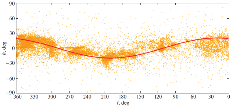
Figure 2: (Color online) Distribution of the PMS3 stars on the celestial sphere; the solid line indicates a cosine wave with an amplitude of 20^∘.

Kinematic Model

From an analysis of the residual velocities $V_{r},V_{l},V_{b}$ we can determine the mean group velocity $U_{G},V_{G},W_{G},$ and four analogs of the Oort constants $A_{G},B_{G},C_{G},K_{G}$ ($G$ is the Gould Belt), which, in our case, characterize the intrinsic rotation ($A_{G}$ and $B_{G}$) and expansion/contraction ($C_{G}$ and $K_{G}$) of the sample of low-mass stars closely associated with the Gould Belt based on the simple Oort–Lindblad kinematic model:

$$\begin{array}[]{lll}V_{r}=U_{G}\cos b\cos l+V_{G}\cos b\sin l+W_{G}\sin b\\ +rA_{G}\cos^{2}b\sin 2l+rC_{G}\cos^{2}b\cos 2l+rK_{G}\cos^{2}b,\end{array}$$ (28)

$$\begin{array}[]{lll}V_{l}=-U_{G}\sin l+V_{G}\cos l\\ +rA_{G}\cos b\cos 2l-rC_{G}\cos b\sin 2l+rB_{G}\cos b,\end{array}$$ (29)

$$\begin{array}[]{lll}V_{b}=-U_{G}\cos l\sin b-V_{G}\sin l\sin b+W_{G}\cos b\\ -rA_{G}\sin b\cos b\sin 2l-rC_{G}\cos b\sin b\cos 2l-rK_{G}\cos b\sin b.\end{array}$$ (30)

We find the unknowns $U_{G},V_{G},W_{G},$ and $A_{G},B_{G},C_{G},K_{G}$ by simultaneously solving the system of conditional equations (28)–(30) by the least-squares method (LSM).

RESULTS

Let us first consider the simplest method of estimating the geometric parameters of the Gould Belt from the distribution of stars on the celestial sphere. Figure 2 presents such a distribution for the PMS3 stars. The cosine wave with an amplitude of $20^{\circ}$ and a phase shift of $20^{\circ}$ is drawn in such a way that the longitude of the ascending node here is $l_{\Omega}=290^{\circ}$. The curve can also be fitted to the data more accurately. However, we should take into account the fact that this is only a projection of stars located at various heliocentric distances onto the sphere. Therefore, an analysis of the spatial coordinates of stars should yield more objective results.

The parameters of the position ellipsoids for three samples of stars are given in Table 1. The principal semiaxes of the position ellipsoid are determined to within a constant. As can be seen from the table, the ellipsoid becomes increasingly elongated along the $x$ axis from PMS1 to PMS3. If the size of the first semiaxis is taken to be 350 pc, then the ellipsoid, for example, for the PMS3 sample will have sizes $350\times 270\times 87$ pc very close to those of the Lindblad ring ($350\times 250\times 50$ pc).

Table 1: Parameters of the position ellipsoids for three samples of stars with relative trigonometric parallax errors less than 15%

Parameters	pms1	pms2	pms3
$N_{\star}$	43706	33978	23683
$\lambda_{1}$	$55.7\pm 0.1$	$49.2\pm 0.1$	$40.4\pm 0.1$
$\lambda_{2}$	$47.7\pm 0.1$	$40.2\pm 0.1$	$31.3\pm 0.1$
$\lambda_{3}$	$17.7\pm 0.1$	$14.0\pm 0.3$	$10.0\pm 0.1$
$\lambda_{1}:\lambda_{2}:\lambda_{3}$	$1:0.86:0.32$	$1:0.82:0.29$	$1:0.77:0.25$
$l_{1},b_{1}$	$~{}35.7\pm 0.5^{\circ},$ $~{}11.0\pm 0.1^{\circ}$	$~{}38.6\pm 0.7^{\circ},$ $12.1\pm 0.2^{\circ}$	$~{}35.0\pm 1.2^{\circ},$ $14.3\pm 0.6^{\circ}$
$l_{2},b_{2}$	$125.4\pm 0.5^{\circ},$ $~{}-2.0\pm 0.1^{\circ}$	$127.9\pm 0.9^{\circ},$ $-3.1\pm 0.1^{\circ}$	$124.5\pm 0.6^{\circ},$ $-2.0\pm 0.2^{\circ}$
$l_{3},b_{3}$	$206.1\pm 0.5^{\circ},$ $~{}78.9\pm 0.1^{\circ}$	$203.8\pm 0.9^{\circ},$ $77.5\pm 0.1^{\circ}$	$206.8\pm 0.6^{\circ},$ $75.6\pm 0.3^{\circ}$

Table 2: Parameters of the residual velocity ellipsoids for three samples of stars using only their propermotions (the upper part of the table) and in the simultaneous solution with the addition of line-of-sight velocities whose errors do not exceed 2 km s^-1 (the lower part of the table)

Parameters	pms1	pms2	pms3
$N_{\star}$	43706	33978	23683
$\sqrt{\sigma_{0}},$ km s-1	$8.7$	$7.7$	$6.9$
$\sigma_{1},$ km s-1	$10.20\pm 0.09$	$9.55\pm 0.10$	$8.70\pm 0.12$
$\sigma_{2},$ km s-1	$7.21\pm 0.12$	$5.96\pm 0.16$	$4.72\pm 0.23$
$\sigma_{3},$ km s-1	$3.86\pm 0.04$	$3.36\pm 0.05$	$2.93\pm 0.05$
$L_{1},B_{1}$	$~{}90\pm 2^{\circ},$ $~{}~{}2\pm 0^{\circ}$	$~{}98\pm 4^{\circ},$ $~{}~{}3\pm 1^{\circ}$	$111\pm 7^{\circ},$ $~{}~{}3\pm 1^{\circ}$
$L_{2},B_{2}$	$179\pm 1^{\circ},$ $-8\pm 1^{\circ}$	$187\pm 1^{\circ},$ $-15\pm 1^{\circ}$	$200\pm 2^{\circ},$ $-31\pm 2^{\circ}$
$L_{3},B_{3}$	$196\pm 1^{\circ},$ $~{}82\pm 1^{\circ}$	$199\pm 1^{\circ},$ $~{}74\pm 1^{\circ}$	$206\pm 2^{\circ},$ $~{}59\pm 1^{\circ}$
$N_{\star}$	41081	32125	22480
$\sqrt{\sigma_{0}},$ km s-1	$9.7$	$8.5$	$7.5$
$\sigma_{1},$ km s-1	$10.58\pm 0.08$	$9.76\pm 0.08$	$8.87\pm 0.10$
$\sigma_{2},$ km s-1	$8.47\pm 0.10$	$7.04\pm 0.14$	$5.58\pm 0.20$
$\sigma_{3},$ km s-1	$3.79\pm 0.03$	$3.33\pm 0.03$	$3.03\pm 0.04$
$L_{1},B_{1}$	$~{}77\pm 1^{\circ},$ $~{}~{}4\pm 0^{\circ}$	$~{}95\pm 2^{\circ},$ $~{}~{}~{}3\pm 1^{\circ}$	$112\pm 3^{\circ},$ $~{}~{}~{}2\pm 0^{\circ}$
$L_{2},B_{2}$	$167\pm 2^{\circ},$ $-6\pm 1^{\circ}$	$184\pm 2^{\circ},$ $-12\pm 1^{\circ}$	$202\pm 2^{\circ},$ $-22\pm 1^{\circ}$
$L_{3},B_{3}$	$197\pm 2^{\circ},$ $~{}83\pm 1^{\circ}$	$200\pm 2^{\circ},$ $~{}~{}78\pm 1^{\circ}$	$208\pm 2^{\circ},$ $~{}~{}68\pm 1^{\circ}$

Table 3: The parameters of the Oort–Lindblad kinematic model that we found based on two samples of stars only from the stars with line-of-sight velocities (upper part) and from all data (lower part)

Parameters	ums		pms3
	before correction	after correction	before correction	after correction
$N_{\star}$	13092	13092	1877	1877
$\sigma_{0},$ km s-1	12.7	12.4	10.1	9.9
$U_{\odot}/U_{G},$ km s-1	$6.43\pm 0.11$	$6.52\pm 0.11$	$5.25\pm 0.24$	$7.56\pm 0.24$
$V_{\odot}/V_{G},$ km s-1	$8.23\pm 0.11$	$3.95\pm 0.11$	$11.82\pm 0.24$	$-0.18\pm 0.24$
$W_{\odot}/W_{G},$ km s-1	$7.22\pm 0.11$	$-0.21\pm 0.11$	$5.36\pm 0.23$	$1.14\pm 0.23$
$V,$ km s-1	$12.70\pm 0.11$	$7.63\pm 0.11$	$14.00\pm 0.24$	$7.65\pm 0.24$
$l,$ deg.	$52\pm 1$	$31\pm 1$	$66\pm 1$	$9\pm 2$
$b,$ deg.	$35\pm 1$	$-2\pm 1$	$23\pm 1$	$9\pm 3$
$A,$ km s-1 kpc-1	$12.01\pm 0.35$	$-3.50\pm 0.35$	$14.38\pm 0.96$	$-0.64\pm 0.95$
$B,$ km s-1 kpc-1	$-7.89\pm 0.35$	$3.39\pm 0.33$	$-16.48\pm 0.92$	$-4.21\pm 0.91$
$C,$ km s-1 kpc-1	$-2.78\pm 0.35$	$-7.18\pm 0.35$	$-4.02\pm 0.95$	$-9.17\pm 0.94$
$K,$ km s-1 kpc-1	$6.42\pm 0.37$	$0.77\pm 0.36$	$5.76\pm 1.00$	$0.12\pm 0.99$
$l_{xy},$ deg.	$5\pm 1$	$-32\pm 1$	$8\pm 2$	$-43\pm 3$
$N_{\star}$	71594	71594	23668	23668
$\sigma_{0},$ km s-1	10.1	9.7	4.3	3.9
$U_{\odot}/U_{G},$ km s-1	$7.56\pm 0.05$	$5.35\pm 0.05$	$10.30\pm 0.05$	$2.55\pm 0.04$
$V_{\odot}/V_{G},$ km s-1	$8.36\pm 0.05$	$3.66\pm 0.05$	$12.61\pm 0.04$	$-0.62\pm 0.04$
$W_{\odot}/W_{G},$ km s-1	$7.03\pm 0.04$	$-0.09\pm 0.04$	$6.02\pm 0.03$	$0.79\pm 0.03$
$V,$ km s-1	$13.28\pm 0.05$	$6.49\pm 0.05$	$17.35\pm 0.04$	$2.75\pm 0.04$
$l,$ deg.	$47.9\pm 0.2$	$34.4\pm 0.4$	$5.8\pm 0.2$	$346\pm 2$
$b,$ deg.	$32.0\pm 0.2$	$-0.8\pm 0.3$	$20.3\pm 0.1$	$17\pm 1$
$A,$ km s-1 kpc-1	$10.45\pm 0.15$	$-4.84\pm 0.14$	$7.01\pm 0.12$	$-7.20\pm 0.11$
$B,$ km s-1 kpc-1	$-11.26\pm 0.11$	$0.32\pm 0.11$	$-16.72\pm 0.10$	$-3.83\pm 0.09$
$C,$ km s-1 kpc-1	$-3.70\pm 0.15$	$-8.68\pm 0.14$	$4.61\pm 0.15$	$0.22\pm 0.14$
$K,$ km s-1 kpc-1	$2.98\pm 0.26$	$-2.48\pm 0.25$	$7.03\pm 0.32$	$1.31\pm 0.29$
$l_{xy},$ deg.	$10\pm 1$	$-30\pm 1$	$-17\pm 1$	$1\pm 1$

We can judge the inclination typical for the Gould Belt by the angles $b_{1}$ and $b_{3}.$ It can be seen from Table 1 that the inclinations deduced from the PMS1 and PMS2 samples are small, 11–12^∘, they are quite far from the expected values. This suggests that the samples are contaminated by background stars and that it is difficult to separate two layers of stars—the layer of Gould Belt nonmembers lying in the Galactic plane and the inclined layer of Gould Belt members. The inclination of 14^∘ found from the PMS3 sample is not very large either. The position of the third axis of the ellipsoid allows the longitude of the ascending node of the PMS3 stellar system to be determined, $l_{\Omega}=l_{3}+90^{\circ}=297\pm 1^{\circ}$.

Table 2 gives the parameters of the residual velocity ellipsoids for three samples of stars. When forming them, we took into account the peculiar solar motion and the differential Galactic rotation in Eqs. (2)–(4). The solution was obtained by two methods. The results obtained only from the stellar proper motions are given in the upper part of the table, while the results obtained from the same stars, but the equation for the line-of-sight velocity (whose errors do not exceed 2 km s^-1), if available, is also used, are given in the lower part of the table.

When using only the stellar proper motions, we obtain the solution with the smallest errors of the parameters being determined. In this case, however, we slightly underestimate them, because we assumed the line-of-sight velocities to be zero when calculating the velocities $U,V,$ and $W$ and the corresponding errors (see Eqs. (20) and (21)). Therefore, the results obtained by invoking the stellar line-of-sight velocities should be deemed more reliable. The results obtained from the PMS3 sample are of greatest interest. In particular, note the position of the first axis of the velocity ellipsoid $L_{1}=112\pm 3^{\circ},$ which is closely related to the direction toward the kinematic center. For example, if we are dealing with the intrinsic rotation of the stellar system (in the absence of intrinsic expansion), then $L_{1}$ should point exactly to the expansion center. Conversely, in the presence of intrinsic expansion (and zero rotation) the direction $L_{1}$ will differ by 45^∘ from the direction toward the system’s kinematic center (Ogorodnikov 1965).

Figure 3 presents the distribution of the PMS3 stars in the $xy,xz,$ and $yz$ planes. The stellar position ellipsoid is shown. Note that the mean coordinates $({\overline{x}},{\overline{y}},{\overline{z}})=(-65,-79,-35)$ pc calculated from the entire PMS3 sample provide information about the concentration center of the sample stars. As can be seen from the figure, the ellipse center was moved along the y axis and placed in the region of the lowest concentration of stars. In this case, the direction to the ellipse center is in good agreement with the direction $L_{1}=112^{\circ}$ found by analyzing the residual velocity ellipsoid as a presumed direction to the kinematic center of the stellar system (Table 2). We clearly see from Fig. 3b that it is desirable to impart a slightly larger inclination to the ellipse. Thus, the inclination $B_{2}=22\pm 1^{\circ}$ found from our analysis of the residual velocity ellipsoid is closer to the value typical for the Gould Belt

To estimate the effects of intrinsic rotation and expansion/contraction of the stellar systems under consideration, we solve the system of conditional equations (28)–(30) by the LSM. We seek its solution based on two samples, UMS and PMS3, both without and with allowance for the influence of the spiral density wave.

The results are presented in Table 3. The model parameters are given in the first column, in the second and fourth columns the velocities were not freed from any effects, and in the third and fifth columns the stellar velocities were freed from the solar motion, the differential Galactic rotation, and the influence of the spiral density wave. Using the parameters $A$ and $C$ found, we calculated the angle $l_{xy}$ (vertex deviation) according to the well-known relation

$${\rm\tan}(2l_{xy})=-C/A,$$

which is valid in the absence of expansion. This angle specifies the direction to the kinematic center of the stellar system.

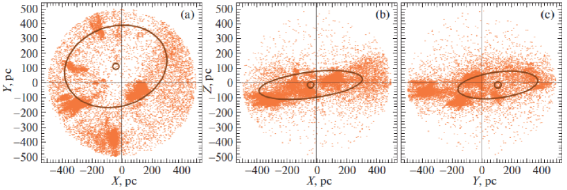
Figure 3: (Color online) Spatial distribution of the PMS3 stars; the ellipsoid was found by analyzing the positions of these stars.

The kinematic equations (28)–(30) were solved by two methods. The results obtained from the stars with complete information, i.e., the parallax, two proper motion components, and line-of-sight velocity are known for each star, are presented in the upper part of Table 3, while the results obtained from the stars with incomplete information, i.e., only the stellar proper motions were used in the absence of line-of-sight velocities, are presented in the lower part of Table 3.

Since the velocities in the second and fourth columns are free from the corrections, the velocities $U_{\odot},V_{\odot}$ and $W_{\odot}$ have the ordinary meaning of the sample group velocity. In contrast, the solar velocity relative to the local standard of rest (LSR) with the values from Schönrich et al. (2010), ($(U,V,W)_{\odot}=(11.1,12.2,7.3)$ km s^-1, was taken into account in the third and fifth columns; therefore, $U_{G},V_{G},W_{G},$ $V,$ $l$ and $b$ show the motion of the entire sample relative to the LSR. Here, the velocity is $V=\sqrt{U^{2}_{G}+V^{2}_{G}+W^{2}_{G}}$ and its direction is $l_{G}$ and $b_{G}.$ The values of these quantities strongly depend on the adopted peculiar solar velocity relative to the LSR. For example, based on open star clusters younger than 60 Myr from the Gould Belt, Bobylev (2004) found $(U,V,W)_{G}=(1.1,-11.8,1.3)$ km s^-1, $l_{G}=275^{\circ}$ and $b=6^{\circ},$, where the peculiar solar velocity components $(U,V,W)_{\odot}=(10.0,5.3,7.2)$ km s^-1 from Dehnen and Binney (1998) were used.

Similarly, in the second and fourth columns the Oort constants $A$ and $B,$ to a lesser degree $C$ and $K,$ describe the differential Galactic rotation, while in the third and fifth columns these parameters already reflect exclusively the intrinsic kinematic properties of the sample stars.

An analysis of the results in Table 3 shows that allowance for the spiral density wave removes almost completely the positive $K$ effect (the expansion of the stellar system). Furthermore, a positive intrinsic rotation of the system with the angular velocity $B-A$ is observed in the residual stellar velocities (the third and fifth columns) and only from the PMS3 sample; in the upper part of the table this rotation is negative (i.e., it coincides in direction with the Galactic one) and has $B-A=-3.57\pm 1.34$ km s^-1 kpc^-1. Strictly speaking (Ogorodnikov 1965), it should be slightly different, because there is a large value of the constant C here; therefore, $A_{\rm new}=\sqrt{A^{2}+C^{2}},$ and then $B-A_{\rm new}=5.0\pm 1.6$ km s^-1 kpc^-1. Thus, the rotation will be positive for the direction to the center $-43^{\circ}$ if in Eqs. (28)–(30) we substitute $l-(-43^{\circ})$ for $l.$ The direction $l_{xy}=-43\pm 3^{\circ}$ here can be interpreted as the fact that the direction to the center of the stellar system is on the line with longitudes $317-137^{\circ}$, with the direction $l=137^{\circ}$ pointing to the second Galactic quadrant, where the center of the Gould Belt is most likely located. In contrast, in the lower part of the table the intrinsic rotation of the PMS3 sample is positive with $B-A=3.37\pm 0.14$ km s^-1 kpc^-1 at an almost zero value of the constant $C.$

The results from Table 3 obtained from the young massive stars of the UMS sample are of interest. There is a positive $K$ effect in their uncorrected velocities, which is removed after allowance for the spiral density wave. For the stars of this sample the errors per unit weight $\sigma_{0}$ are noticeably larger. Since in the catalogue by Zari et al. (2018) the stars were selected with a fairly strong restriction on the absolute value of the tangential velocity, $V_{t}<40$ km s^-1, the Galactic rotation parameters ($A$ and $B$ in the second column of the table) may be underestimated.

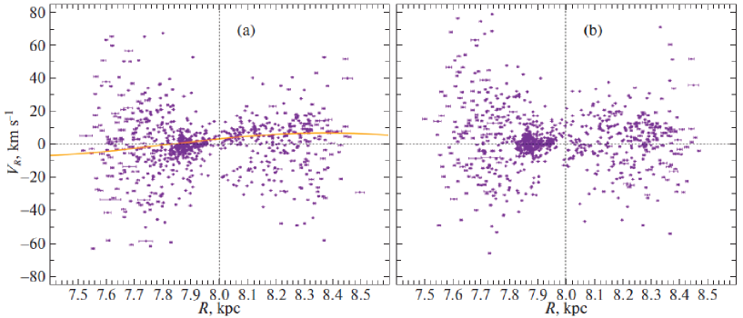
Figure 4: (Color online) Galactocentric radial velocities, $V_{R},$ of the PMS3 stars versus distance $R$ corrected for the solar motion (a) and for the Galactic rotation and the spiral density wave (b).

As we see from Fig. 1, the stars with line-of-sight velocities in both samples under consideration occupy slightly different regions on the H–R diagram compared to the entire sample. Thus, they have a slightly different evolutionary status. Most likely, there is a significant fraction of type-A stars among the stars with measured line-of-sight velocities in the UMS sample (the dark circles in Fig. 1a). In contrast, there is a large fraction of faint stars in the PMS3 sample without line-of-sight velocities (the light circles in Fig. 1b), where the parallax and proper motion errors increase significantly compared to the brighter stars from the Gaia DR2 catalogue. From this viewpoint, the differences in kinematic parameters between the upper and lower parts of the table should come as no surprise.

As a result, in our opinion, the most reliable values of the derived kinematic parameters are contained in the fourth and fifth columns of the upper part of Table. 3. These parameters were deduced from the PMS3 sample. It is also interesting to note that the group velocity of this sample shows a close association with the Gould Belt. Indeed, as can be seen from the last column of the table, the velocity $V$ has a direction $l$ from 179^∘ to 166^∘ and $b$ from $-9^{\circ}$ to $-17^{\circ}$, i.e., it lies virtually in the plane of the Gould Belt.

Figure 4 presents the Galactocentric radial velocities $V_{R}$ of the PMS3 stars. In the first case (Fig. 4a), they were corrected only for the solar motion. An inclined arrangement of points is clearly seen in the immediate solar neighborhood with a radius of about 200 pc. This graph shows the wave

$$-7\cos\biggl{[}-{2\pi R_{0}\over 2.2}\ln\biggl{(}{R\over R_{0}}\biggr{)}-120^{\circ}\biggr{]},$$

written according to relations (6) and (7), with a perturbation amplitude $f_{R}=7$ km s^-1, a wavelength $\lambda=2.2$ kpc, and the Sun’s phase in the wave $\chi_{\odot}=-120^{\circ}.$ Here the minus in front of the formula means that at the center of the spiral arm (for example, at $R\approx 7.2$ kpc) the perturbation is directed toward the Galactic center.

In the second case (Fig. 4b), the velocities corrected for the solar motion, the differential Galactic rotation, and the influence of the spiral density wave are given. As can be seen from the figure, allowance for all these effects makes the distribution of points horizontal. Interestingly, the densest clump of points in Fig. 4 at $R\approx 7.9$ kpc formed by stars from the Scorpio–Centaurus OB association also becomes more horizontal after allowance for the influence of the spiral density wave. However, the local inclination still remains, suggesting the presence of intrinsic expansion of this association.

DISCUSSION

Based on OB stars from the Hipparcos catalogue (1997) younger than 60 Myr, Torra et al. (2000) determined the inclination, 16–22^∘, and the longitude of the ascending node of the great circle, 275–295^∘. Bobylev (2016) showed that the system of nearby high-latitude molecular clouds could be fitted by an ellipse with sizes $350\times 235\times 140$ pc oriented at an angle of $17\pm 2^{\circ}$ to the Galactic plane with a longitude of the ascending node of $337\pm 1^{\circ}$. Since high-latitude molecular clouds very far from the symmetry plane of the Gould Belt were considered, the third axis of this ellipsoid turned out to be unusually large.

Dzib et al. (2018) analyzed twelve star-forming regions containing young stars and closely associated with the Gould Belt. Kinematic data from the Gaia DR2 catalogue were used. They showed that this system could be fitted by an ellipsoid with sizes $358\times 316\times 70$ pc and the center in the second Galactic quadrant $(x,y,z)_{0}=(-82,39,-25)\pm(15,7,4)$ pc. The ellipsoid is oriented at an angle of $21\pm 1^{\circ}$ to the Galactic plane with a longitude of the ascending node of $319\pm 2^{\circ}$. A new estimate of the Gould Belt expansion velocity was also obtained from these data, $2.5\pm 0.1$ km s^-1.

Having analyzed a large sample of clump giants from the Gaia DR2 catalogue, Gontcharov (2019) determined the inclination of the dust layer associated with the Gould Belt, $18\pm 2^{\circ}$. In addition, he estimate the scale height of this dust layer to be $170\pm 40$ pc. Thus, the geometric characteristics of the PMS3 stars found in this paper (an inclination of $14-22^{\circ}$ and a longitude of the ascending node of the great circle $297-298^{\circ}$) are in good agreement with the characteristics of the Gould Belt determined by various authors from other data. This suggests that the overwhelming majority of young T Tauri stars from the PMS3 sample belong to the Gould Belt structure.

It is interesting to estimate the $K$ effect in angular units. By definition, $2K=V_{R}/R+\partial V_{R}/\partial R$ if the rotation velocity $V_{\theta}$ is independent of the angle $V_{\theta},$ $\partial V_{\theta}/\partial\theta=0$ (Ogorodnikov 1965). Then, at a constant angular velocity (i.e., at $\partial V_{R}/\partial R=0$) $\partial V_{R}/\partial R=0$ and $2K=V_{R}/R$.

From our examination of a wave similar to that in Fig. 4 we find $2K=2f_{R}/(\lambda/2)$ and, consequently, $K=4.5$ km s^-1 kpc^-1. In this case, we should take into account the fact that the correction strongly depends on the Sun’s phase $\chi_{\odot}$. Thus, even if the influence of the Galactic spiral density wave is taken into account, the Gould Belt can have a slight residual expansion. For example, having analyzed OB stars from the Hipparcos catalogue younger than 30 Myr, Lindblad et al. (1997) obtained an estimate of $K=12$ km s^-1 kpc^-1. Based on OB stars younger than 60 Myr, Torra et al. (2000) found $K=7.1\pm 1.4$ km s^-1 kpc^-1. Based on a sample of young stars, Bobylev (2004) found $K=8\pm 2$ km s^-1 kpc^-1.

The probability that there is an intrinsic expansion of the Scorpio–Centaurus association even after allowance for the influence of the spiral density wave is great. For example, Blaauw (1964) found the expansion coefficient for it to be $K=50$ km s^-1 kpc^-1. Based on a sample of young stars with data from the Hipparcos catalogue, Bobylev and Bajkova (2007) refined this coefficient, $K=46\pm 8$ km s^-1 kpc^-1. As can be seen from Fig. 4, the stars of this association exert a strong influence on the K estimate for the Gould Belt. When analyzing young massive multiple systems, Bobylev and Bajkova (2013) noted a significant radial velocity gradient $V_{R}/R\sim 40$ km s^-1 kpc^-1 in the region of the Scorpio–Centaurus association. They suggested that the influence of the spiral density wave should be eliminated before determining the intrinsic expansion parameters of the Scorpio–Centaurus association. Indeed, as can be clearly seen from Fig. 4, the spiral density wave and the velocities of the Scorpio–Centaurus association are almost parallel to one another; therefore, it is difficult to separate one effect from the other.

The residual velocity dispersions of the PMS3 stars are low, for example, $\sigma_{0}=7.5$ km s^-1 (Table 2),and the principal semiaxes of the residual velocity ellipsoid $\sigma_{1,2,3}=(8.87,5.58,3.03)\pm(0.10,0.20,0.04)$ km s^-1 are comparable to the velocity dispersion of the gas clouds belonging to the Gould Belt, 1–5 km s^-1 (Galli et al. 2019).

CONCLUSIONS

We studied the spatial and kinematic properties of a large sample of young pre-main stars. For this purpose we used the catalogue by Zari et al. (2018) containing more than 40 000 T Tauri stars with their proper motions and parallaxes from the Gaia DR2 catalogue. We also considered the kinematic properties of a large (more than 80 000) sample of young stars (these are stars of spectral types O, B, and A) from this catalogue that occupy the upper part on the H–R diagram. The line-of-sight velocities are known for some of these stars.

We validated the hypothesis of Zari et al. (2018) that the stars belonging to the PMS3 sample have a very close spatial and kinematic association with the Gould Belt. The following characteristics of the position ellipsoid were estimated from the coordinates of thePMS3 stars: its sizes are $350\times 270\times 87$ pc and it is oriented at an angle of $14\pm 1^{\circ}$ to the Galactic plane with a longitude of the ascending node of $297\pm 1^{\circ}$.

Our analysis of the motions of PMS3 stars showed that the residual velocity ellipsoid with principal semiaxes $\sigma_{1,2,3}=(8.87,5.58,3.03)\pm(0.10,0.20,0.04)$ km s^-1 is oriented at an angle of $22\pm 1^{\circ}$ to the Galactic plane with a longitude of the ascending node of $298\pm 2^{\circ}$.

We showed that much ($\sim$5–7 km s^-1 kpc^-1) of the expansion effect (K effect) typical for Gould Belt stars could be explained by the influence of a Galactic spiral density wave. When making allowance for the influence of the spiral density wave, we took into account only the radial velocity perturbation component $f_{R}=5$ km s^-1 by assuming that it made a major contribution when allowing for the $K$ effect. After allowance for the peculiar solar motion relative to the LSR, the differential Galactic rotation, and the density wave in the residual stellar velocities, the intrinsic expansion becomes very small or even is replaced by contraction. At the same time, an intrinsic rotation with an magnitude of 3–6 km s^-1 kpc^-1 manifests itself, with the sign of this rotation being most likely positive. This effect should be studied further in more detail.

ACKNOWLEDGMENTS

I am grateful to the referee for the useful remarks that contributed to an improvement of the paper.

FUNDING

This work was supported in part by Program KP19–270 of the Presidium of the Russian Academy of Sciences “Questions of the Origin and Evolution of the Universe with the Application of Methods of Ground-Based Observations and Space Research”.

REFERENCES

1. A. Blaauw, Ann. Rev. Astron. Astrophys. 2, 213 (1964).

2. V. V. Bobylev, Astron. Lett. 30, 784 (2004).

3. V. V. Bobylev, Astron. Lett. 32, 816 (2006).

4. V. V. Bobylev, Astrophysics 57, 583 (2014).

5. V. V. Bobylev and A. T. Bajkova, Astron. Lett. 33, 571 (2007).

6. V. V. Bobylev and A. T. Bajkova, Astron. Lett. 39, 532 (2013).

7. V. V. Bobylev and A. T. Bajkova, Astron. Lett. 40, 783 (2014).

8. V. V. Bobylev, Astron. Lett. 42, 544 (2016).

9. V. V. Bobylev and A. T. Bajkova Astron. Lett. 43, 452 (2017).

10. V. V. Bobylev and A. T. Bajkova, Astron. Lett. 45, 208 (2019a).

11. V. V. Bobylev and A. T. Bajkova, Astron. Rep. 63, 932 (2019b).

12. A. G. A. Brown, A. Vallenari, T. Prusti, de Bruijne, C. Babusiaux, C. A. L. Bailer-Jones, M. Biermann, D.W. Evans, et al. (Gaia Collab.), Astron. Astrophys. 616, 1 (2018).

13. A. K. Dambis, L. N. Berdnikov, Yu. N. Efremov, A. Yu. Knyazev, A. S. Rastorguev, E. V. Glushkova, V. V. Kravtsov, D. G. Turner, D. J. Majaess, and R. Sefako, Astron. Lett. 41, 489 (2015).

14. T. M. Dame, D. Hartmann, and P. Thaddeus, Astrophys. J. 547, 792 (2001).

15. W. Dehnen and J. J. Binney, Mon. Not. R. Astron. Soc. 298, 387 (1998).

16. S. A. Dzib, L. Loinard, G. N. Ortiz-León, L. F. Rodriguez, and P. A. B. Galli, Astrophys. J. 867, 151 (2018).

17. Yu.N. Efremov, Sites of Star Formation inGalaxies (Nauka, Moscow, 1989) [in Russian].

18. D. Fernández, F. Figueras, and J. Torra, Astron. Astrophys. 372, 833 (2001).

19. P. A. B. Galli, L. Loinard, H. Bouy, L. M. Sarro, G. N. Ortiz-León, S. A. Dzib, J. Olivares, M. Heyer, et al., Astron. Astrophys. 630, 137 (2019).

20. G. A. Gontcharov, Astron. Lett. 45, 605 (2019).

21. C. C. Lin and F. H. Shu, Astrophys. J. 140, 646 (1964).

22. P. O. Lindblad, Bull. Astron. Inst. Netherland 19, 34 (1967).

23. P. O. Lindblad, J. Palouš, K. Loden, and L. Lindegren, in HIPPARCOS Venice’97, Ed. by B. Battrick (ESA Publ. Div., Noordwijk, 1997), p. 507.

24. P. O. Lindblad, Astron. Astrophys. 363, 154 (2000).

25. L. Lindegren, J. Hernandez, A. Bombrun, S. Klioner, U. Bastian, M. Ramos-Lerate, A. de Torres, H. Steidelmuller, et al. (Gaia Collab.), Astron. Astrophys. 616, 2 (2018).

26. A. V. Loktin and M. E. Popova, Astrophys. Bull. 74, 270 (2019).

27. Yu. N.Mishurov and I. A. Zenina, Astron. Astrophys. 341, 81 (1999).

28. K. F. Ogorodnikov, Dynamics of Stellar Systems (Fizmatgiz, Moscow, 1965; Pergamon, Oxford, 1965).

29. C. A. Olano, Astron. Astrophys. 121, 295 (2001).

30. C. A. Perrot and I. A. Grenier, Astron. Astrophys. 404, 519 (2003).

31. A. E. Piskunov, N. V. Kharchenko, S. Röser, E. Schilbach, and R.-D. Scholz, Astron. Astrophys. 445, 545 (2006).

32. W.G. L. Pöppel, Fundam. Cosmic Phys. 18, 1 (1997).

33. W. G. L. Pöppel, ASP Conf. Ser. 243, 667 (2001).

34. A. S. Rastorguev, M. V. Zabolotskikh, A. K. Dambis, N. D. Utkin, V. V. Bobylev, and A. T. Bajkova, Astrophys. Bull. 72, 122 (2017).

35. M. J. Sartori, J. R. D. Lepine, andW. S. Dias, Astron. Astrophys. 404, 913 (2003).

36. R. Schönrich, J. Binney, and W. Dehnen, Mon. Not. R. Astron. Soc. 403, 1829 (2010).

37. The HIPPARCOS and Tycho Catalogues, ESA SP–1200 (1997).

38. J. Torra, D. Fernández, and F. Figueras, Astron. Astrophys. 359, 82 (2000).

39. C. A. O. Torres, R. Quast, C. H. F. Melo, and M. F. Sterzik, Handbook of Star Forming Regions, Vol. 2,, Vol. 5 of The Southern Sky ASPMonograph Publications, Ed. by Bo Reipurth (ASP, San Francisco, 2008).

40. R. J. Trumpler and H. F. Weaver, Statistical Astronomy (Univ. of Calif. Press, Berkely, 1953).

41. O. O. Vasilkova, Astron. Lett. 40, 59 (2014).

42. E.Zari, H. Hashemi, A.G. A. Brown, K. Jardine, and P. T. de Zeeuw, Astron. Astrophys. 620, 172 (2018).

43. P. T. de Zeeuw, R. Hoogerwerf, J. H. J. de Bruijne, A. G. A. Brown, and A. Blaauw, Astron. J. 117, 354 (1999).