First Light And Reionisation Epoch Simulations
(FLARES) I: Environmental Dependence of High-Redshift Galaxy Evolution

Abstract

We introduce the First Light And Reionisation Epoch Simulations (Flares), a suite of zoom simulations using the Eagle model. We resimulate a range of overdensities during the Epoch of Reionisation (EoR) in order to build composite distribution functions, as well as explore the environmental dependence of galaxy formation and evolution during this critical period of galaxy assembly. The regions are selected from a large $(3.2\;\mathrm{cGpc})^{3}$ parent volume, based on their overdensity within a sphere of radius $14$ h^-1 cMpc. We then resimulate with full hydrodynamics, and employ a novel weighting scheme that allows the construction of composite distribution functions that are representative of the full parent volume. This significantly extends the dynamic range compared to smaller volume periodic simulations. We present an analysis of the galaxy stellar mass function (GSMF), the star formation rate distribution function (SFRF) and the star forming sequence (SFS) predicted by Flares, and compare to a number of observational and model constraints. We also analyse the environmental dependence over an unprecedented range of overdensity. Both the GSMF and the SFRF exhibit a clear double-Schechter form, up to the highest redshifts ($z=10$). We also find no environmental dependence of the SFS normalisation. The increased dynamic range probed by Flares will allow us to make predictions for a number of large area surveys that will probe the EoR in coming years, carried out on new observatories such as Roman and Euclid.

1 Introduction

A goal of numerical galaxy evolution studies is to model a representative population of galaxies, resolving all of the relevant physics at the required scales, in order to provide a test bed for the study and interpretation of observed galaxies (Benson, 2010). In order to achieve this it is necessary to simulate large volumes (in order to sample a representative volume of the Universe) at high resolution (e.g. spatial, mass, time; in order to resolve the internal physical processes within individual galaxies) and with all of the key physics included (such as full hydrodynamics, magnetic fields, etc.). Unfortunately this is not computationally feasible; compromises must be made with volume, resolution or choice of physics, depending on the scientific questions posed (for a review, see Somerville & Davé, 2015).

The most common approach to obtain a representative population of galaxies is to simulate a large periodic cube, tens of Mpc across on a side. This approach has been used in a number of leading projects to simulate large volumes down to redshift zero, producing thousands of galaxies across a wide range of stellar masses. Projects such as Eagle (Schaye et al., 2015; Crain et al., 2015), Simba (Davé et al., 2019), Illustris (Vogelsberger et al., 2014; Genel et al., 2014), Illustris-TNG (Pillepich et al., 2017; Nelson et al., 2017), Romulus (Tremmel et al., 2016) and Horizon-AGN (Dubois et al., 2014) have mass resolutions of order $10^{6}\mathrm{M_{\odot}}$, sufficiently high to resolve the internal structure of galaxies. However, despite these large volumes, the rarest peaks of the overdensity distribution are still poorly sampled due to the lack of large scale modes in constrained periodic volumes. Much larger volumes are required to sample the rare overdensities on large scales that are likely to evolve in to the most massive clusters by the present day. For example, the Eagle simulation contains just 7, relatively low-mass clusters ($M_{200,c}>10^{14}\,\mathrm{M_{\odot}}$) at $z=0$ within the fiducial 100 Mpc volume (Schaye et al., 2015).

One means of overcoming the limitations of relatively small periodic volumes is to use much larger, dark matter-only simulations, with box lengths of order Gpc, as sources for zoom simulations. These use regions selected from the dark matter only simulation as source initial conditions, and resimulate them at higher resolution with extra physics, such as full hydrodynamics (Katz & White, 1993; Tormen et al., 1997). This technique preserves the large scale power and tidal forces by simulating the dark matter at low resolution outside the high resolution region. A recent example is the C-Eagle simulations, high-resolution hydrodynamic simulations of 30 clusters with a range of descendant masses (Barnes et al., 2017b; Bahé et al., 2017). These were selected from a parent dark matter simulation with volume $(3.2\;\mathrm{cGpc})^{3}$ (Barnes et al., 2017a). This enormous volume contains $185\,150$ clusters ($\mathrm{M_{200,c}}>10^{14}\,\mathrm{M_{\odot}}$) and $1701$ high-mass clusters ($\mathrm{M_{200}}>10^{15}\,\mathrm{M_{\odot}}$). The C-Eagle zoom approach allowed the application of the Eagle model to cluster environments, without having to simulate a large periodic box.

The zoom technique can also be used to sample a range of overdensities, not just the peaks of the overdensity distribution. The GIMIC simulations (Crain et al., 2009) are one example of this approach; they picked 5 different regions of radius $20$ h^-1 cMpc  at $z=1.5$ from the Millennium simulation (Springel et al., 2005), with overdensities (-2,-1,0,1,2)$\sigma$ from the cosmic mean at z = 1.5. These were then resimulated at high resolution with full hydrodynamics. This not only allowed the investigation of the environmental effect of galaxy evolution, without having to simulate a whole periodic box, but also, by appropriately weighting each region according to its overdensity, the regions could be combined to produce composite distribution functions. These composite functions have much larger dynamic range than those obtained from smaller periodic boxes, and at much lower computational expense than running a large periodic volume.

In this paper we use a similar approach to GIMIC to produce composite distribution functions of galaxy intrinsic properties, but focused on the Epoch of Reionisation (EoR). The EoR approximately covers the first 1.2 billion years of the Universe’s history ($4\leqslant z\leqslant 15$), from the birth of the first Population III stars, to when the majority of the intergalactic medium is ionized (Bromm & Yoshida, 2011; Zaroubi, 2013; Stark, 2016; Dayal & Ferrara, 2018; Cooray et al., 2019). A number of surveys over the past 15 years, with both space- and ground-based observatories, have discovered thousands of galaxies during this epoch (Beckwith et al., 2006; Warren et al., 2007; Wilkins et al., 2011; Koekemoer et al., 2011; Grogin et al., 2011; McCracken et al., 2012; Bouwens et al., 2015). Using intervening clusters as gravitational lenses has pushed the measurement of luminosity functions to even fainter magnitudes (Castellano et al., 2016; Livermore et al., 2017; Atek et al., 2018; Ishigaki et al., 2018). Spectral energy distribution fitting has been used to characterise the intrinsic properties of these galaxies, measuring for example their stellar masses (e.g. Gonzalez et al., 2011; Duncan et al., 2014; Song et al., 2016; Stefanon et al., 2017) and star formation rates (e.g. Smit et al., 2012; Katsianis et al., 2017). However, we have yet to unambiguously detect Population III stars (Yoshida, 2019), and the first stages of galaxy assembly are yet to be probed, particularly the seeding and early growth of super massive black holes (Smith et al., 2017).

However, this situation may soon change with the introduction of a number of new observatories, each with unique capabilities for exploring the EoR. JWST will provide unprecedented sensitive imaging with NIRCam, and follow up spectroscopy with NIRSpec and MIRI, to detect and characterise potentially the very first forming galaxies in the Universe (Gardner et al., 2006). In tandem, Roman and Euclid will produce wide-field surveys of the EoR (Spergel et al., 2015; Laureijs et al., 2011). These surveys will predominantly probe the bright end of the rest-frame UV Luminosity Function (UVLF), which is currently poorly constrained by periodic hydrodynamic simulations due to their small volume. They will also discover some of the most extreme galaxies, in terms of luminosity and intrinsic mass, in the observable Universe at these redshifts (Behroozi & Silk, 2018). These observations will be important to constrain models of galaxy formation and evolution, but it is also possible to predict observed populations in advance and test the recovery of intrinsic parameters (Pforr et al., 2012, 2013; Smith & Hayward, 2015; Lower et al., 2020).

Predictions for upcoming wide-field surveys have so far typically been made using phenomenological models. One such class of methods are Semi-Analytic Models (SAMs), run on halo merger trees extracted from dark matter-only simulations (for a review, see Baugh, 2006). Due to their efficiency they can be applied to large cosmological volumes, and used to probe distribution functions of intrinsic properties and observables over a large dynamic range. A number of these models have been tested during the EoR (Henriques et al., 2015; Clay et al., 2015; Somerville et al., 2015; Poole et al., 2016; Rodrigues et al., 2017; Yung et al., 2019b; Lagos et al., 2019). Mock observables can also be produced and directly compared with observed luminosity functions (Lacey et al., 2016; Yung et al., 2019a; Vijayan et al., 2019). Such models can be run relatively quickly, allowing parameter estimation through Monte Carlo approaches (Henriques et al., 2015), a powerful means of exploring large degenerate parameter spaces. However, despite recent progress in resolving SAM galaxies in to multiple components (e.g. Henriques et al., 2020), such models necessarily do not self-consistently model physical processes on small scales, relying on analytic recipes.

Most existing periodic hydrodynamic simulations during the EoR are not able to achieve the large dynamic ranges accessible by SAMs. This is illustrated in Figure 1, which shows where a number of existing simulations lie on a plane of simulated volume against hydrodynamic element mass. There is a strong negative correlation, with some outliers. The BlueTides simulation (Feng et al., 2016, 2015), based on the Massive Black suite of simulations (Matteo et al., 2012; Khandai et al., 2015), was performed within a (500  / h cMpc)³ periodic box, $\sim$125 times as massive as the fiducial Eagle volume, whilst at a similar resolution. They make predictions for a number of intrinsic and observational properties during the EoR (e.g. Waters et al., 2016; Di Matteo et al., 2017; Wilkins et al., 2016b, a, 2017, 2018; Wilkins et al., 2020) Unfortunately, due to the increased computational cost it has only been run down to $z=7$, and the model cannot therefore be tested against low redshift observables. Other simulations have taken a different approach, instead simulating smaller volumes at much higher resolution, allowing them to investigate the effect of a number of physical processes in greater detail (O’Shea et al., 2015; Jaacks et al., 2019). However, these must similarly be stopped at intermediate redshifts due to the higher computational expense.

In this paper we introduce Flares, zoom resimulations during the EoR using the Eagle model. The Eagle project (Schaye et al., 2015; Crain et al., 2009) is a suite of Smoothed Particle Hydrodynamics (SPH) simulations, calibrated to reproduce the stellar mass function and sizes of galaxies in the local Universe. Eagle has been shown to be in good agreement with a large number of observables not used in the calibration (e.g. Lagos et al., 2015; Bahé et al., 2016; Furlong et al., 2017; Trayford et al., 2015, 2017; Crain et al., 2017). This includes predictions at high-redshift: Furlong et al. (2015) found reasonably good agreement with observationally inferred distribution functions of stellar mass and star formation rate out to $z=7$. Unfortunately, there are very few galaxies in the fiducial Eagle volume during the EoR. This is particularly the case for the most massive objects, which predominantly reside in protocluster environments, the progenitors of today’s collapsed clusters (Chiang et al., 2017; Lovell et al., 2018). Flares allows us to significantly increase the number of galaxies simulated during the EoR with Eagle. It also allows us to test the already incredibly successful Eagle model in a new regime of extreme, high-$z$ environments, whilst still resolving hydrodynamic processes at $10^{6}\,M_{\odot}$ resolution, and provide predictions for a number of key upcoming observatories.

In this, the first Flares paper, we introduce the resimulation method, our suite of zoom simulations, and present our first predictions for the distribution of galaxies by stellar mass and star formation rate using the composite approach. This is the first in a series of papers studying the galaxy properties in the Flares sample; in Paper II we forward-model the full spectro-photometric properties, and predict the UV luminosity function and its high redshift evolution (Vijayan et al., in prep.). We assume a Planck year 1 cosmology ($\Omega_{0}=0.307$, $\Omega_{\Lambda}=0.693$, $h=0.6777$, Planck Collaboration et al., 2014) and a Chabrier stellar initial mass function (IMF) throughout (Chabrier, 2003), and have corrected observational results accordingly.

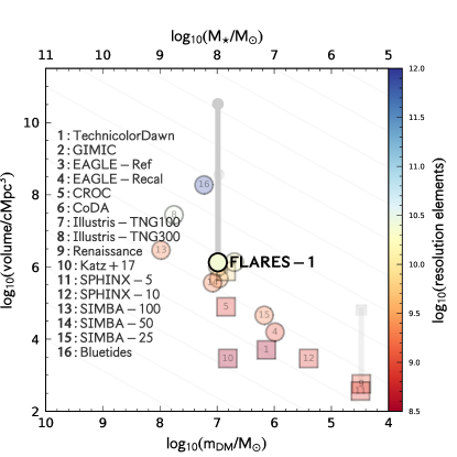
Figure 1: Dark matter element resolution against simulated volume. The colour of individual points describes the approximate number of resolution elements (dark matter + baryonic gas, excluding stars). We show the following simulation projects: Technicolor Dawn (Finlator et al., 2018), GIMIC (Crain et al., 2009), EAGLE (Schaye et al., 2015; Crain et al., 2015), CROC (Gnedin, 2014), CoDa (Ocvirk et al., 2016), Illustris (Vogelsberger et al., 2014), Renaissance (Barrow et al., 2017), the Katz et al. (2017) simulations, SPHINX (Rosdahl et al., 2018), and BlueTides (Feng et al., 2016). We also show Flares with the total resimulated high-resolution volume, as well as a vertical line showing the representative volume, given by that of the parent box. There is a strong negative correlation for periodic volumes between the volume that can be simulated and the resolution that can be achieved. The resimulation approach, with appropriate weighting, allows us to extend the volume axis significantly.

2 The Flare Simulations

We will now detail our simulations, including the Eagle model, selection of the regions, the zoom resimulation technique, and our method for constructing composite distribution functions.

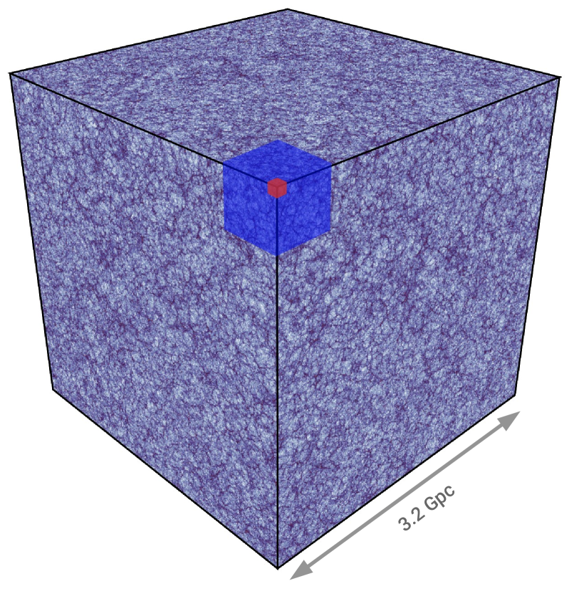
Figure 2: Diagram of the 3.2 cGpc box from which we select our regions (Barnes et al., 2017a). To demonstrate the increase in volume, we show the Bluetides simulation ($L=570$ cMpc; Feng et al., 2016) inset in blue, and the fiducial EAGLE simulation ($L=100$ cMpc; Schaye et al., 2015) inset in red.

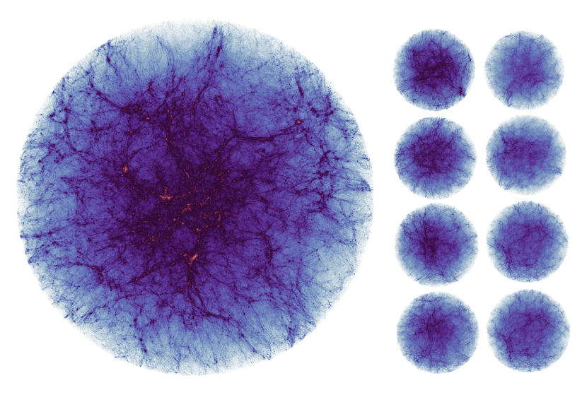
Figure 3: Visualisation of the dark matter integrated density in a number of resimulation regions of differing overdensity ($\delta$), made with Py-SPHViewer (Benitez-Llambay, 2015). The region on the left shows the most overdense region ($00$, $\delta=0.970$). The regions to the right are (anticlockwise from top left) $17$, $20$, $22$, $24$, $26$, $28$, $30$, $38$, with overdensities $\delta=[0.616,0.266,0.121,-0.007,-0.121,-0.222,-0.311,-0.479]$, respectively.

2.1 The Eagle Model

The Eagle physics model is based on that developed for the OWLS project (Schaye et al., 2010), which is a heavily modified version of P-Gadget-3 (Springel et al., 2005), an $N$-body tree-PM SPH code. The hydrodynamics suite is collectively known as ‘Anarchy’, (described in Appendix A of Schaye et al. (2015), and Schaller et al. (2015)). In short, it consists of the Hopkins (2013) pressure-entropy SPH formalism, an artifical viscosity switch (Cullen & Dehnen, 2010), an artificial conductivity switch (e.g. Price, 2008), the Wendland (1995) $C^{2}$ smoothing kernel with 58 neighbours, and the Durier & Dalla Vecchia (2012) time-step limiter.

Radiative cooling, formation of stars, black hole seeding, and feedback from stars and black holes are all handled by subgrid models. Full details are provided in Schaye et al. (2015); Crain et al. (2015). We use the AGNdT9 parameter configuration, which produces similar mass functions to the reference model but better reproduces the hot gas properties in groups and clusters (Barnes et al., 2017b). This is identical to that used in the C-Eagle simulations, but differs from the fiducial Reference simulation (see Table 1). It uses a higher value for $C_{\mathrm{visc}}$, which controls the sensitivity of the BH accretion rate to the angular momentum of the gas, and a higher gas temperature increase from AGN feedback, $\Delta T$. A larger $\Delta T$ leads to fewer, more energetic feedback events, whereas a lower $\Delta T$ leads to more continual heating. These parameter changes impact the central black hole accretion, which has been shown to be efficient only at halo masses $>\,10^{12}\,M_{\odot}$ (Bower et al., 2017). At $z=10$ no Flares galaxies reside in such halos, however at $z=5$ a minority do ($<0.2\%$), which may affect the early star formation histories of cluster galaxies (Bahé et al., 2017). We use an identical resolution to the fiducial Eagle simulation, with gas particle mass $m_{g}=1.8\times 10^{6}\;\mathrm{M_{\odot}}$, and a softening length of $2.66\;\mathrm{ckpc}$.

Table 1: Variation of subgrid parameters between models.

Simulation Prefix	$C_{\mathrm{visc}}$	$\Delta T_{\mathrm{AGN}}$
		$\mathrm{[K]}$
Ref	$2\pi$	$10^{8.5}$
AGNdT9	$2\pi\times 10^{2}$	$10^{9}$

2.2 Region Selection

We use the same parent simulation as that used in the C-Eagle simulations (Barnes et al., 2017a): a (3.2 cGpc)³ dark matter-only simulation with a particle mass of $8.01\,\times\,10^{10}$ M_⊙, using a Planck Collaboration et al. (2014) cosmology. Figure 2 shows a diagram of the box compared to the fiducial Eagle reference volume, as well as the BlueTides simulation (Feng et al., 2016). The highest redshift snapshot available for this simulation is at $z=4.67$, which we use for our selection. Within this snapshot, we select spherical volumes that sample a range of overdensities. By taking a sufficiently large radius we can ensure that the density fluctuations averaged on that scale are linear, such that the distortion in the shape of the Lagrangian volume during the simulation will not be too extreme and that the ordering of the density fluctuations is preserved. The regions, and their overdensities, are given in Table 4.

To determine the density, we first distribute the mass onto a high resolution, $3.2\;\mathrm{cGpc}\,/\,1200\sim 2.67\;\mathrm{cMpc}$ cubic grid using a nearest grid point assignment scheme. We then find the density on larger scales by convolving the grid with a spherical top-hat filter of radius $14$ h^-1 cMpc. We find, in test volumes, that this gives densities very close to those calculated from the raw particle data. The overdensity is then defined as

$$\delta(\textbf{x})=\frac{\rho(\textbf{x})}{\bar{\rho}}-1,$$ (1)

where $\rho$ is the density at grid coordinates x, and $\bar{\rho}$ is the mean density in the box. The upper panel of Figure 4 shows the distribution of overdensity in log-space, alongside a fitted log-normal distribution.

We select regions for resimulation with two different goals: firstly, we select a number of regions of high overdensity in order to obtain a large sample of the first massive galaxies to form in the Universe; and secondly we select regions with a range of overdensities in order to explore the environmental impact (bias) on galaxy formation. In order to achieve the first goal we select the 16 most overdense regions in the volume, which have $\delta\geqslant 0.8$. For the second goal, we select two regions at each overdensity based on their rms overdensity $\sigma$, in the range $\sigma\in[4,3,2,1,0.5,0,-0.5,-1,-2,-3]$. We choose two regions of each overdensity in order to minimise the effect of cosmic variance at fixed overdensity; we also select an additional two mean density regions, to increase the sampled volume of these common regions. Finally, we also select the two most underdense regions ($\delta\sim-0.45$) in order to cover the whole dynamic range. This gives a total of 40 regions. Figures 9 and 12 show the overdensity dependence of the GSMF and SFRF, respectively; at fixed overdensity the poisson noise is low, which suggests the effect of cosmic variance is low, and that the number of regions chosen was sufficient to demonstrate the trends presented in this article. However, we plan to run a greater number of simulations to further reduce the noise above the knee of the stellar mass function; an advantage of the resimulation approach is that this can simply be achieved by running more simulations to increase the total simulated volume.

The selected regions are listed in Appendix A and the range of overdensities that each covers (evaluated at each point on the 2.67 cMpc grid enclosed by that volume) is shown in the lower panel of Figure 4. We discuss how to combine the resimulations so as to obtain a representative sample of the whole Universe in Section 2.4.

2.3 The Resimulation Method

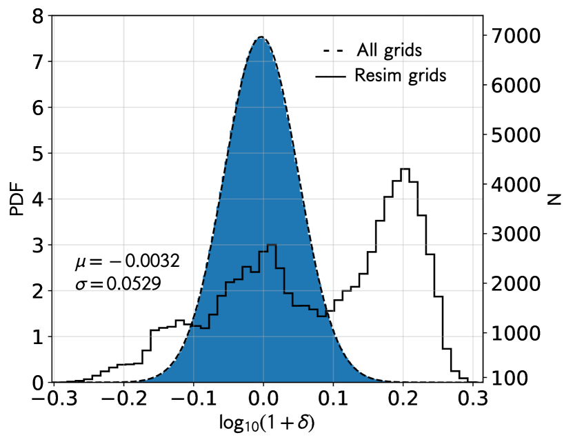
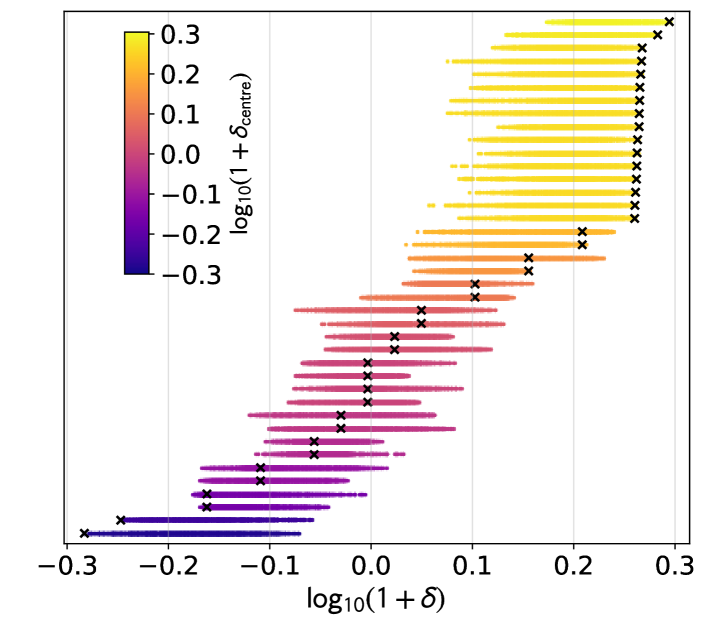
Figure 4: Upper panel: the probability distribution function of sampled overdensities. The dashed black line shows a lognormal fit with the given parameters. The solid blue histogram shows the grid locations that lie within one of our resimulation volumes. The solid black histogram shows the distribution of our selected regions in overdensity, binned into 50 equal width bins, with the right y-axis showing only their number counts. Lower panel: the distribution of overdensities within each simulation volume. The vertical displacement is arbitrary. The cross shows the overdensity measured at the centre of the resimulated volume and the spread of values shows the overdensities within each volume evaluated at each point on the 2.67 cMpc grid.

Galaxies on the edge of the high resolution region will not be modelled correctly due to the presence of a pressureless boundary. To avoid this we resimulate a region 15 h^-1 cMpc  in radius, and ignore all galaxies within 1 h^-1 cMpc  of the edge of the sphere in post-processing. At higher redshift the Lagrangian high resolution region can deform, but we found that it is close to spherical out to the highest redshifts considered in this work ($z=10$). Figure 3 shows the dark matter distribution within the cutout radius for a range of resimulations of differing overdensity, at $z=4.7$. We also show the fiducial periodic Eagle volume to provide a visual comparison of the differing environments probed.

As in the standard Eagle analysis, structures are first found using a Friends-Of-Friends (FOF, Davis et al., 1985) finder, then split into bound substructures using the Subfind algorithm (Springel et al., 2001). Their properties are then defined using those stellar particles within 30 pkpc of the location of the most tightly-bound stellar particle. We limit our analysis to galaxies sampled by at least 50 star particles, which corresponds to a mass limit of approximately $\mathrm{log_{10}}(M_{\star}\,/\,\mathrm{M_{\odot}})\geqslant 7.95$.

2.4 Distribution Function Weighting

In this section we describe how we combine our resimulations to obtain a statistically-correct representation of the universal cosmological distribution of galaxies. As we show below in Section 3.2, distribution functions, such as the galaxy stellar mass function, vary with the overdensity of the resimulated volume. Therefore, it is necessary to weight each resimulation to reproduce the correct distribution of those overdensities averaged over the whole Universe, i.e. the cosmic mean.

As mentioned in Section 2.2, the overdensity within spherical top-hat regions of radius 14 h^-1 cMpc  is sampled on a 2.67 cMpc grid; we label this sample $\delta_{g}$. Since the grid sampling is finer than the size of the resimulation volume, each resimulation volume is associated with just under 2000 different values of $\delta_{g}$. We show the distribution of those $\delta_{g}$ within each resimulation volume in the lower panel of Figure 4. The most overdense regions, whilst containing a single highly overdense point, in fact contain points covering a range of overdensities. It is, therefore, important to account for this spread in sampled overdensity, rather than just using the central overdensity when determining the contribution from any particular resimulation volume.

The top panel of Figure 4 contrasts the PDFs of $\delta_{g}$ for the whole box and for our resimulated sample. To generate the correct mean distibutions, we divide into bins of overdensity as shown by the histogram in Figure 4 (black solid line), then weight the resimulations appropriately to reproduce the cosmic distribution. Specifically, we do the following:

• The overdensity domain is split up into 50 bins of equal width in $\log_{10}(1+\delta)$, $i=1\ldots N_{\delta}$. For each of these, it is possible to assign a weight, $w_{\mathrm{true},i}$, in proportion to the fraction of $\delta_{g}$ that lie in that bin, such that $\Sigma_{i}w_{\mathrm{true},i}=1$.

• Each resimulation, $j$, is similarly distributed over these overdensity bins with weights, $w_{ij}$, in proportion to the enclosed values of $\delta_{g}$. Thus $\Sigma_{i}w_{ij}=1$.

• The sample weight associated with each bin is $w_{\mathrm{sample},i}=\Sigma_{j}w_{ij}$.

• To obtain the correct universal average, we therefore have to weight each density bin by the ratio $r_{i}=w_{\mathrm{true},i}/w_{\mathrm{sample},i}$.

Ideally, we would associate each galaxy with the local value of $\delta_{g}$. However, for the purposes of simplicity in this paper, we give all galaxies within a particular resimulation equal weight – this will give some dispersion over the more correct method, which we will implement in a future paper.

• Hence we adjust the contribution of each resimulation by a factor $f_{j}=\Sigma_{i}r_{i}w_{ij}$.

We note that

$$\Sigma_{j}f_{j} =\Sigma_{j}\Sigma_{i}r_{i}w_{ij}=\Sigma_{i}r_{i}\Sigma_{j}w_{ij}$$

$$=\Sigma_{i}r_{i}w_{\mathrm{sample},i}=\Sigma_{i}w_{\mathrm{true},i}=1.$$ (2)

These simulation weighting factors are listed in Table 4.

We further note that, at higher redshifts, the overdensities will evolve. Nevertheless, because even the most extreme perturbations are only mildly non-linear, we would expect that the ordering of the overdensities would largely be preserved. Hence, we use the same sampling at all redshifts. That also allows for a much more direct comparison of the evolution within each overdensity sample.

3 Results

3.1 Galaxy Number Counts

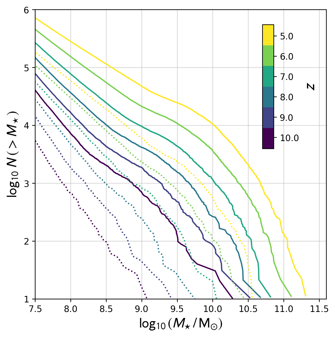
Figure 5: Cumulative distribution of stellar masses for all Flares regions combined (solid) and the fiducial Eagle Reference volume (dashed).

We begin by examining the raw number counts of galaxies. Figure 5 shows the cumulative distribution function of galaxies with stellar mass for both Flares and the Reference periodic volume ($V=(100\,\mathrm{cMpc})^{3}$). We produce over $\sim 20$ times more $10^{10}\,\mathrm{M_{\odot}}$ galaxies at $z=5$ than obtained in the 100 cMpc periodic volume, despite the fact that the total high-resolution volume of all resimulated regions is only 50% larger than the periodic volume. This confirms that the first galaxies are significantly biased to higher overdensity regions.

3.2 The Galaxy Stellar Mass Function

The Galaxy Stellar Mass Function (GSMF) describes the number of galaxies per unit volume per unit stellar mass interval d$\log_{10}M$,

$$\phi(M)=N\,/\,\mathrm{Mpc^{-3}\,dex^{-1}}\;\;,$$ (3)

and is commonly described using a Schechter function (Schechter, 1976),

$$\phi(M)\,\mathrm{d}\log_{10}M=\mathrm{ln}(10)\,\phi^{*}\,e^{-M/M^{*}}\,\left(\frac{M}{M^{*}}\right)^{\alpha+1},$$ (4)

which describes the high- and low-mass behaviour with an exponential and a power law dependence on stellar mass, respectively. Recent studies have found that a double Schechter function can better fit the full distribution (e.g. the GAMA survey, Baldry et al., 2008).

$$\phi(M)\,\mathrm{d}\log_{10}M =\mathrm{ln}(10)\,e^{-M/M^{*}}\times$$

$$\left[\,\phi^{*}_{1}\,\left(\frac{M}{M^{*}}\right)^{\alpha_{1}+1}+\phi^{*}_{2}\,\left(\frac{M}{M^{*}}\right)^{\alpha_{2}+1}\right].$$ (5)

The low mass slope of the second schechter function contributes to only a very narrow dynamic range. Above this range the exponential dominates, and below this the low mass slope of the first schechter function dominates. It is therefore poorly constrained by the binned data, and so as not to introduce further degrees of freedom into our fit we fix it at $\alpha_{2}=-1$. We define the stellar mass $M_{\star}$ as the total mass of all star particles, associated with the bound subhalo, within a 30 kpc aperture (proper) centred on the potential minimum of the subhalo.

3.2.1 The cosmic GSMF

In this section, we present results for the universal GSMF, averaged within our (3.2 cGpc)³ box. This is obtained by combining the individual GSMFs from each of our resimulation volumes with appropriate weighting, as described in Section 2.4.

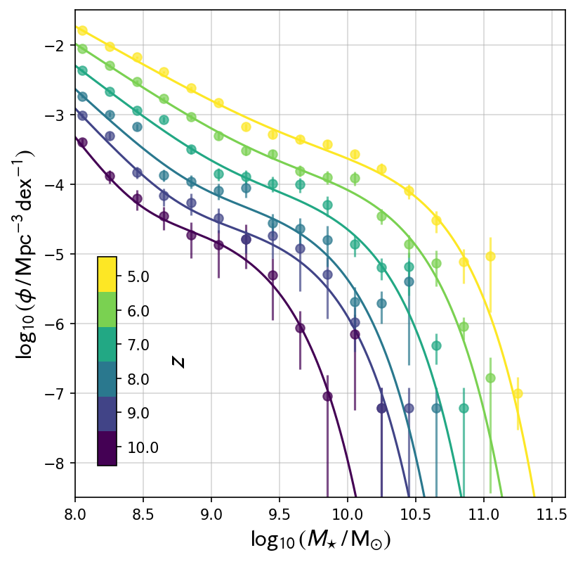
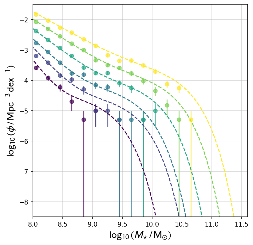
Figure 6: Top: Redshift evolution of the Flares composite galaxy stellar mass function. Points show binned differential counts with Poisson $1\sigma$ uncertainties from the simulated number counts. Solid lines show double-Schechter function fits, quoted in Table 6. The parameter evolution is shown in Figure 7. Bottom: as for the top panel, but points show the counts from the periodic Reference volume. The dashed lines show the double-Schechter fitted relation from Flares. The coverage of the massive end in the periodic volume is poor.

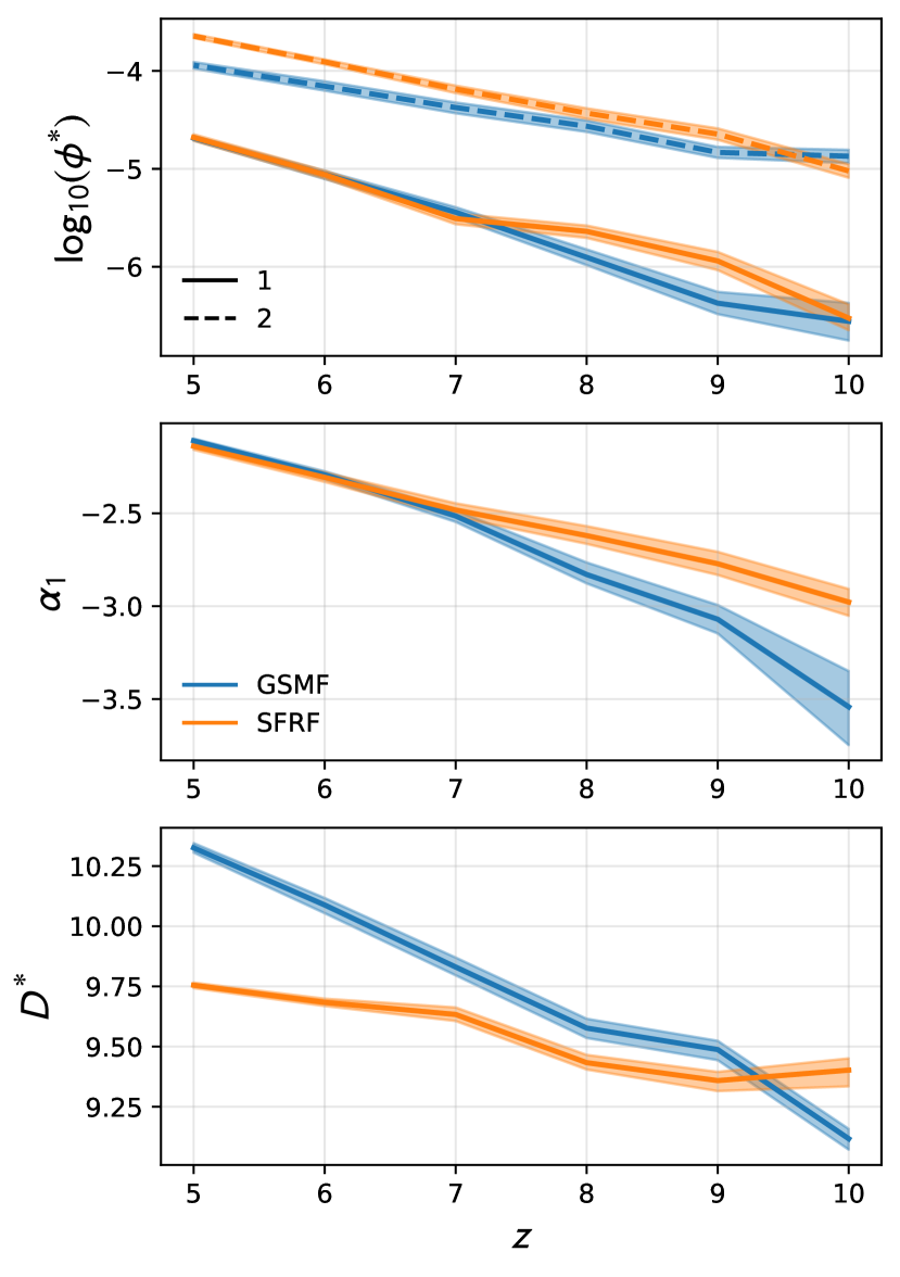
Figure 7: Parameter evolution for double-Schechter function fits to the Flares composite galaxy stellar mass function (GSMF, blue) and star formation rate function (SFRF, orange). The low (1) and high (2) mass components are shown with solid and dashed lines, respectively. Shaded regions show the $16^{\mathrm{th}}-84^{\mathrm{th}}$ percentile uncertainty obtained from the fit posteriors (see Appendix C for details) The low-mass slope of the high-mass component ($\alpha_{2}$) is fixed at -1. The characteristic mass of the GSMF ($\mathrm{M_{\star}}$) and the characteristic SFR of the SFRF ($\psi_{*}$) are shown in the bottom panel, labelled $D_{*}$. $\psi_{*}$ is offset by $+10^{8}$ to aid comparison with $M_{\star}$. The GSMF and SFRF show very similar behaviour; the normalisation of both components and the low-mass slope all increase with decreasing redshift. The characteristic mass increases with decreasing redshift for the GSMF, whereas the characteristic star formation rate of the SFRF shows a flatter redshift relation.

The top panel of Figure 6 shows the GSMF for redshifts between $z=10\mapsto 5$. We show differential counts in bins $0.2\,\mathrm{dex}$ in width (with 1$\sigma$ poisson uncertainties). The solid lines show double-Schechter function fits at each integer redshift. The normalisation increases with decreasing redshift, and the characteristic mass (or knee) of the distribution shifts to higher masses. This is more clearly seen in Figure 7, which shows the evolution of the double-Schechter parameters with redshift. The low-mass slope also gets shallower with decreasing redshift, from $-3.5$ at $z=10$ to $-2.0$ at $z=5$.

Our composite GSMF significantly extends the dynamic range of the GSMF compared to the periodic volumes. To demonstrate, the bottom panel of Figure 6 shows the Flares double-Schechter fits, alongside the binned counts from the Reference periodic volume. At each redshift the maximum stellar mass probed is approximately an order of magnitude larger in Flares. In fact, the periodic reference volume barely probes the exponential tail of the high mass component of the GSMF. When fitting a double-Schechter to the binned Reference volume counts we found that the parameters of the high mass component were completely unconstrained. However, it is clear from the bottom panel of Figure 6 that the low-mass slope is consistent between the Reference volume and Flares. We have also tested that this is the case for the $(50\;\mathrm{Mpc})^{3}$ AGNdT9 periodic volume. This provides evidence that our weighting method is accurately recovering the composite GSMF, without suffering from completeness bias. We note that the GSMF in the AGNdT9 and Reference periodic volumes is also in agreement at the low mass end, which gives us confidence that model incompleteness is not affecting our results.

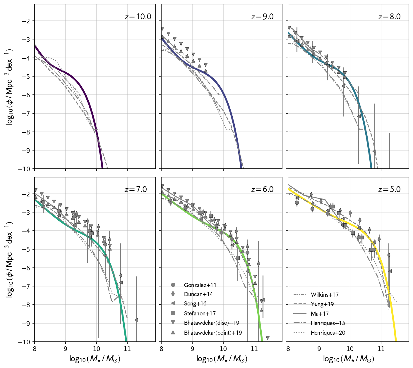
Figure 8: Flares composite galaxy stellar mass function evolution, alongside observational constraints (Gonzalez et al., 2011; Duncan et al., 2014; Song et al., 2016; Stefanon et al., 2017; bhatawdekar_evolution_2018) as well as predictions from other models (Wilkins et al., 2017; Ma et al., 2018; Yung et al., 2019b; Henriques et al., 2015; Henriques et al., 2020). There is some disagreement over the normalisation of the GSMF between different observational studies, however Flares is consistent up to $z=9$.

In Figure 8 we show the composite Flares GSMF against a number of high-$z$ observational constraints in the literature (Gonzalez et al., 2011; Duncan et al., 2014; Song et al., 2016; Stefanon et al., 2017; Bhatawdekar et al., 2019). These studies show a spread of $\sim 0.5\;\mathrm{dex}$ at $z=5$, which highlights the difficulty of accurately measuring the GSMF at high redshift. The Flares composite GSMF lies within this inter-study scatter, most closely following the relations derived by Song et al. (2016) up to $z=7$. At $z\geqslant 8$ observational constraints are limited to cluster lensing studies such as the Hubble Frontier Fields, which do not probe the high-mass end due to the limited volume probed, but can reach very lower stellar masses ($\sim 10^{7}\;M_{\odot}$). The fits presented in Bhatawdekar et al. (2019) have a higher normalisation than in Flares over the accessible mass range, though they quote an uncertainty at $10^{8.5}\;M_{\odot}$ of $\sim 0.6$ dex at $z=9$; Flares lies within this uncertainty for the point sources, but is still in tension with the normalisation for disc-like sources. There is good agreement with the low-mass slope for both sources.

We also compare in Figure 8 to predictions from other galaxy formation models. The Feedback In Realistic Environments (Fire) project performed zoom simulations of individual halos with masses between $10^{8}\;-\;10^{12}\,M_{\odot}$, which were then combined to provide a composite galaxy stellar mass function probing the low-mass regime (Ma et al., 2018). Flares is consistent with Fire at all redshifts where their mass range overlaps. Figure 8 also shows both the 2015 and 2020 versions of L-Galaxies. Both models are in reasonably good agreement at all redshifts shown, but tend to underestimate the number density of massive galaxies at $z=5$ compared to both Flares and the observations.

Yung et al. (2019b) presented results from the Santa Cruz semi-analytic model (Somerville et al., 2015), which extends to a wide dynamic range. Whilst Flares is consistent with this model for $z\leqslant 7$, at $z\geqslant 8$ the Santa Cruz model predicts a more power-law shape to the GSMF, with a lower normalisation at the characteristic mass. This is in agreement with the observed flattening of the GSMF with increasing redshift.

3.2.2 Environmental dependence of the GSMF

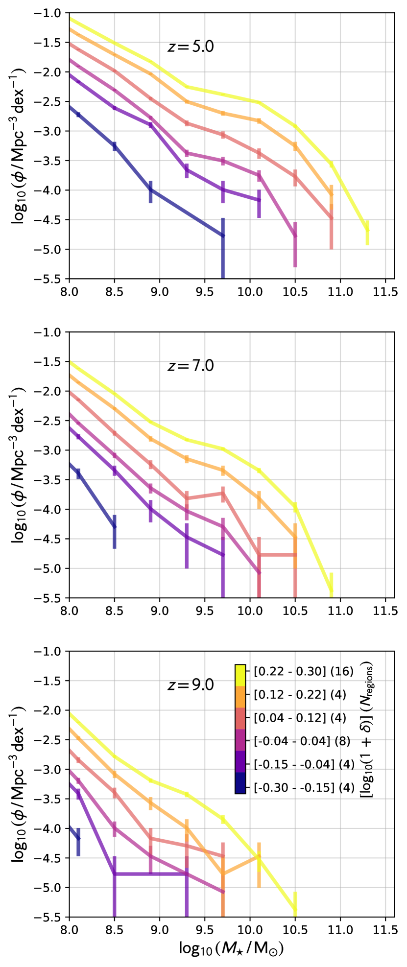
Figure 9: The Flares GSMF between $z=5$ and $9$ split by binned log-overdensity. The binning is shown in the legend, along with the number of regions in each bin. Poisson 1$\sigma$ uncertainties are shown for each bin from the simulated number counts. The normalisation increases with increasing overdensity, and probes higher stellar masses.

Our zoom simulations of a range of overdensities not only allow us to construct a composite GSMF for the entire $(3.2\,\mathrm{Gpc})^{3}$ volume, but also investigate the environmental effect on the GSMF. Section 2 demonstrates the wide range of environments probed, from extremely underdense void regions, to the most overdense high redshift structures that are likely to collapse in to massive, $>10^{15}\;\mathrm{M_{\odot}}$ clusters by $z=0$ (Chiang et al., 2013; Lovell et al., 2018).

Figure 9 shows the GSMF in bins of log-overdensity from $z=5-9$. We use wider bins than previously ($0.4\,\mathrm{dex}$) due to the lower galaxy numbers in each resimulation. As expected, higher overdensity regions have a higher normalisation, $\sim+2\;\mathrm{dex}$ above the lowest overdensity regions at $M_{\star}\,/\mathrm{M_{\odot}}=10^{9.5}\;(z=5)$. There is also an apparent difference in the shape as a function of log-overdensity: lower overdensity regions exhibit a distribution that is more power-law -like, whereas higher overdensity regions clearly show a double-Schechter -like knee. This may be due to the higher number of galaxies in the overdense regions, better sampling the knee, but may also point to differing assembly histories for galaxies in different environments. We will explore the star formation and assembly histories more closely in future work.

The dependence of the GSMF on overdensity may explain the tension between the composite Flares GSMF and other models at $z>7$ seen in Figure 8. Our much larger box allows us to sample extreme overdensities that are not present in smaller volumes. Observationally, the Song et al. (2016) results show a more power law-like form at $z=8$. Double-Schechter forms of the GSMF at low-$z$ have been attributed to the contribution of a passive and star forming population, each fit individually by a single Schechter function (Kelvin et al., 2014; Moffett et al., 2016), though this separation is not perfect (e.g. Ilbert et al., 2013; Tomczak et al., 2016). The robust double-Schechter shape measured in Flares at $z\geqslant 8$ is therefore curious; we see in Appendix B that there is no significant passive population as a function of stellar mass. We therefore tentatively suggest that the tension may be due to the small volume probed observationally at these depths, which does not probe extreme environments that contribute significantly to the cosmic GSMF.

We do not fit each binned GSMF in log-overdensity as there are insufficient galaxies to provide a robust fit. However, we do provide fits to the normalisation at a given stellar mass and redshift, in the following form,

$$\mathrm{log_{10}}\;\phi\,(\mathrm{log_{10}}(1+\delta)\,|\,M_{\star},z)=m\,[\mathrm{log_{10}}(1+\delta)]+c,$$ (6)

where $\mathrm{log_{10}}(1\,+\,\delta)$ is the overdensity of the region. Table 2 shows these fits for bins $\pm 0.2$ dex wide centred at $\mathrm{log_{10}}(M_{\star}\,/\,\mathrm{M_{\odot}})=[8.5,\,9.7]$.

Table 2: Fits to the normalisation, $\log_{10}(\phi/$Mpc^-3dex^-1), of the GSMF at different redshifts and masses (see Section 3.2.2).

$z$	$\mathrm{log_{10}(M_{\star}/M_{\odot})}$	$m$	$c$
5	8.5	3.5	-2.4
7	8.5	4.4	-3.2
9	8.5	4.6	-4.0
5	9.7	4.8	-3.6
7	9.7	4.4	-4.2
9	9.7	4.0	-4.9

3.3 The Star Formation Rate Distribution Function

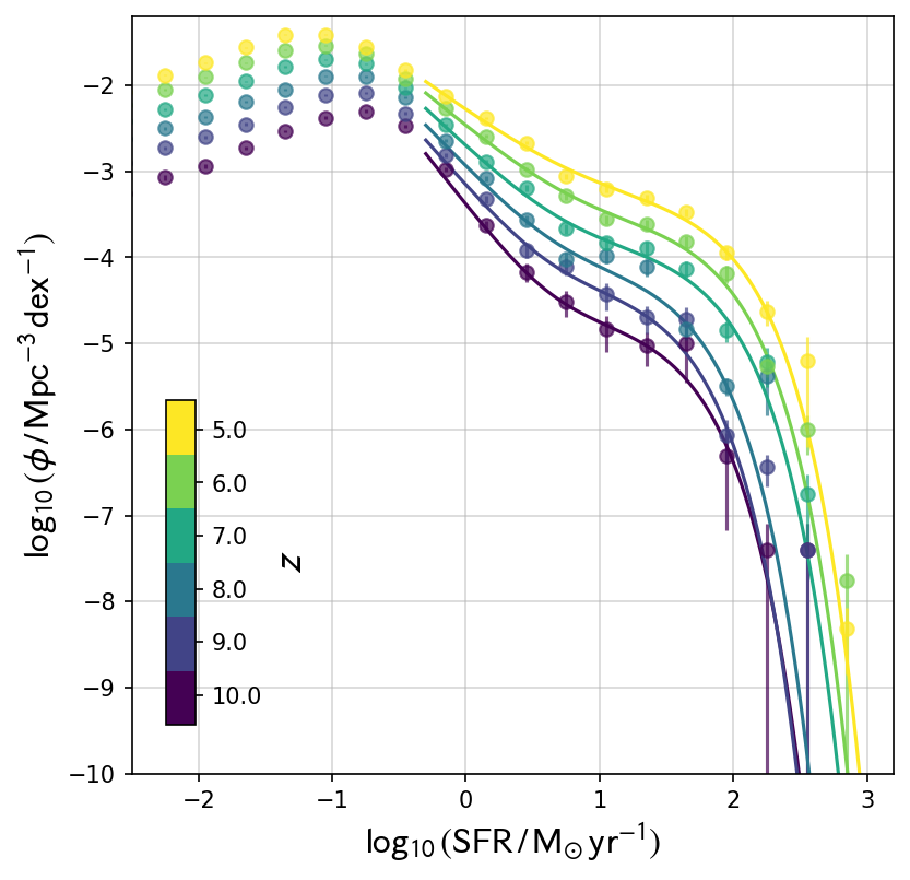
Figure 10: Redshift evolution of the Flares composite star formation rate distribution function. Points show binned differential counts with Poisson 1$\sigma$ uncertainties from the simulated number counts. Solid lines show double-Schechter function fits, quoted in Table 7.

The Star Formation Rate distribution Function (SFRF) describes the number of galaxies per unit volume per unit star formation rate interval d$\log_{10}\psi$, where $\psi$ is the star formation rate,

$$\phi(\psi)=N\,/\,\mathrm{Mpc^{-3}\,dex^{-1}}\;\;.$$ (7)

We define the SFR as the sum of the instantaneous SFR of all star forming gas particles, associated with the bound subhalo, within a 30 kpc aperture (proper) centred on the potential minimum of the subhalo.

3.3.1 The cosmic SFRF

In Figure 10 we plot the evolution of the Flares composite SFRF. We provide counts in bins 0.3 dex in width. There is a clear low-mass turnover between $\sim 0.1\,-\,0.3\,\mathrm{M_{\odot}\;yr^{-1}}$, but above this the shape is well described by a double-Schechter function. Salim & Lee (2012) argue that a single-Schecter is inadequate to describe the SFRF, as we find, though they propose a ’Saunders’ function that does not provide a good fit to the Flares SFRF. We provide fits using the following parametrisation,

$$\phi(\psi)\,\mathrm{d}\log_{10} \psi=\mathrm{ln}(10)\,e^{-\psi/\psi^{*}}\times$$

$$\left[\,\phi^{*}_{1}\,\left(\frac{\psi}{\psi^{*}}\right)^{\alpha_{1}+1}+\phi^{*}_{2}\,\left(\frac{\psi}{\psi^{*}}\right)^{\alpha_{2}+1}\right].$$ (8)

We limit our fits to those galaxies with $\psi>0.5\,\mathrm{M_{\odot}\;yr^{-1}}$; these fits are provided in Table 7. We also plot the parameter evolution with redshift in Figure 7. The characteristic star formation rate, $\psi_{*}$, is offset by $+10^{8}$ to aid comparison with the GSMF characteristic mass, $\mathrm{M_{\star}}$.

The normalisation of both components ($\phi_{1};\,\phi_{2}$), as well as the low-SFR slope ($\alpha_{1}$), increase with decreasing redshift. These trends are surprisingly similar to those seen for the equivalent parameters in the GSMF. The low-SFR normalisation is almost identical, as is the high-SFR normalisation, with a small $\sim+0.2\;\mathrm{dex}$ offset. The low-SFR slope $\alpha_{1}$ is shallower than that of the GSMF at the highest redshifts ($z\geqslant 8$), but identical at lower redshifts. However, the evolution of the characteristic SFR is significantly flatter compared to that of the characteristic mass for the GSMF. This suggests a redshift-independent upper limit to the SFR. The strong correspondence between the shape of the GSMF and the SFRF may be the result of the tight star-forming sequence relation at all redshifts (see Section 3.4).

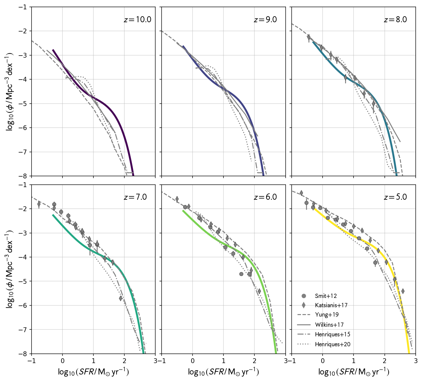
Figure 11: Evolution of the Flares composite star formation rate distribution function (coloured, solid lines), compared with observational constraints from UV data and other model predictions. Smit et al. (2012) derive SFRs from UVLF data, as do Katsianis et al. (2017) using Bouwens et al. (2015) data. Both are corrected to a Chabrier IMF using the conversion factors quoted in Kennicutt Jr & Evans II (2012). The Santa-Cruz SAM (Yung et al., 2019b, dashed line) and BlueTides simulation (Wilkins et al., 2017) show a different behaviour, with a power law shape at higher redshifts, in contrast to the prominent knee seen in Flares up to $z=10$. Both L-Galaxies models also show similar behaviour, though with lower normalisation at the high-SFR end (Henriques et al., 2015; Henriques et al., 2020).

This double-Schechter form of the SFRF is in some tension with observational constraints. Figure 11 shows a comparison with UV derived relations from Smit et al. (2012) and Katsianis et al. (2017) (the latter using Bouwens et al. 2015 data). For low-SFRs the observed normalisation is slightly higher ($\sim\,0.3$ dex) from $z=5$ to $7$. There is no prominent knee in the observed relations, and the exponential tail drops off at lower SFRs than in the simulations.

Figure 11 also shows results from recent cosmological models. As with the GSMF, there is some tension with the SFRF produced by the Santa Cruz models (Yung et al., 2019b). Flares has a distinct double-Schechter shape, whereas the SC model appears as a single schechter at $z=5$, before evolving to a power law at $z=10$. The BlueTides results (Wilkins et al., 2017) also show a similar power law relation at $z\geqslant 8$, in tension with the prominent knee in Flares. Both L-Galaxies models show similar power law-like behaviour, though with lower normalisation at the high-SFR end (Henriques et al., 2015; Henriques et al., 2020), though in better agreement with the existing observational data at $z=6$ compared to the Santa Cruz model and Flares.

The offset in normalisation of the Flares SFRF at high SFRs with the observations may be a selection effect due to highly dust-obscured galaxies. These galaxies, with number densities of $\sim 10^{-5}\;\mathrm{cMpc^{-3}}$ at $z\sim 2$ (Simpson et al., 2014), will be missed in higher redshift rest frame-UV observations. We will perform a direct comparison with the UV luminosity function, including selfconsistent modelling of dust attentuation, in Paper II, Vijayan et al., in prep.. The offset may also be a modelling issue; Eagle was not compared to high redshift observables during calibration, only to data at much lower redshifts ($z=0.1$) than those studied here ($z\geqslant 5$). Improvements to the subgrid modelling at high-redshift, particularly that of star-formation feedback, may improve the agreement.

To investigate what effect our sampling of highly overdense regions has on the composite shape of the SFRF, we now look at the overdensity dependence of the SFRF.

3.3.2 Environmental dependence of the SFRF

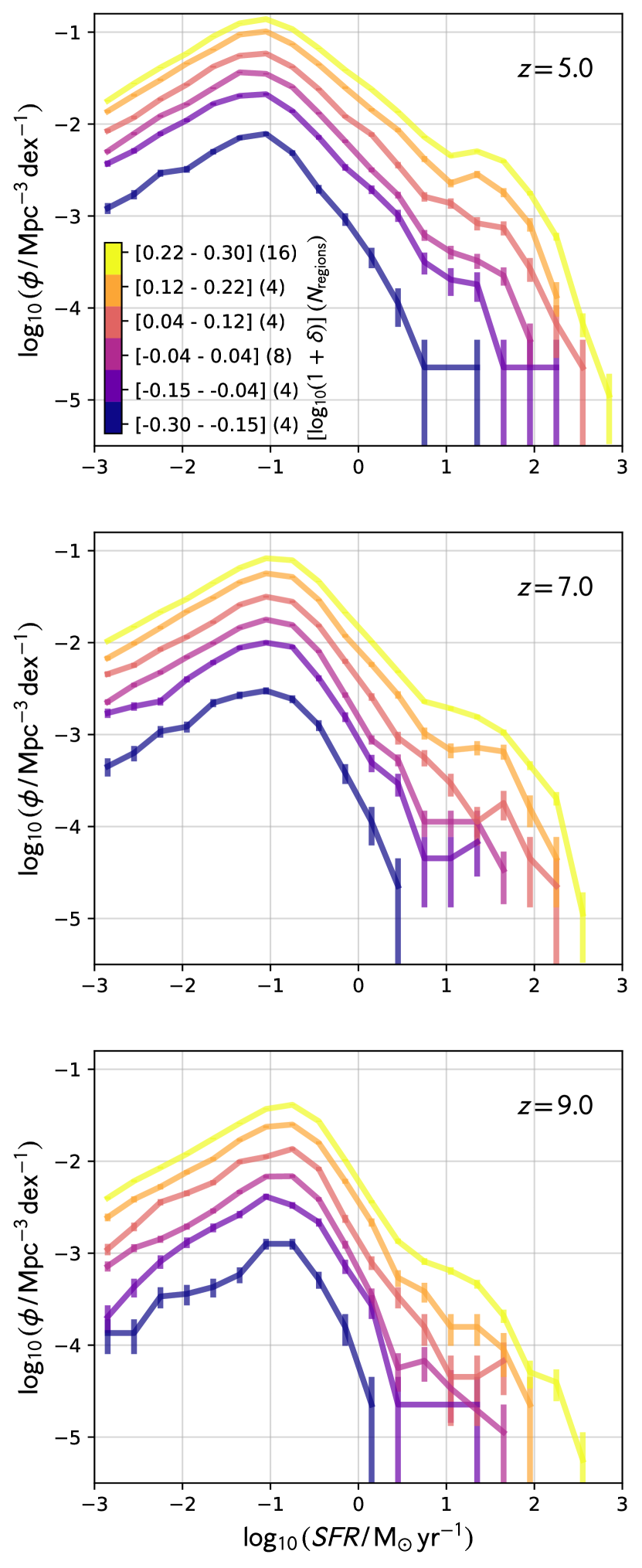
Figure 12: The Flares SFRF between $z=5$ and $9$ split by binned log-overdensity. The binning is shown in the legend, along with the number of regions in each bin. Poisson 1$\sigma$ uncertainties are shown for each bin from the simulated number counts. The normalisation increases with increasing overdensity, and the maximum SFR increases.

Figure 12 shows the SFRF for regions binned by their log-overdensity. There is almost no variation in the shape as a function of overdensity except for the highest overdensities, which show a more prominent double-Schechter knee in the high-SFR regime. This behaviour is identical to that seen for the GSMF. This may explain why the shape of the Flares composite SFRF differs with those of other cosmological models. Flares better samples the rare, high-density regions that contribute significantly to the high-SFR ($\psi>100\,\mathrm{M_{\odot}yr^{-1}}$) tail of the SFRF. Both BlueTides and the Santa-Cruz model are run on regions with much smaller volumes ($500^{3}$ and $357^{3}$ $\mathrm{cMpc^{3}}$, respectively), which may not probe the extreme regions sampled in the Flares parent volume. The mean density region in Figure 12 appears power law-like at all redshifts, which may present a better comparison with these models.

As for the GSMF, we provide fits to the normalisation at a given SFR and redshift, in the following form,

$$\phi\,(\mathrm{log_{10}}(1+\delta)\,|\,\psi,z)=m\,[\mathrm{log_{10}}(1+\delta)]+c,$$ (9)

where $\mathrm{log_{10}}(1\,+\,\delta)$ is the overdensity of the region. Table 3 shows these fits for bins $\pm 0.2$   dex wide centred at $\mathrm{log_{10}}(\psi\,/\,\mathrm{M_{\odot}}\,yr^{-1})=[-0.5,\,0.5]$. The normalisation increases with increasing overdensity as expected. The trends with redshift are also broadly similar to those seen for the GSMF.

Table 3: Fits to the normalisation, $\log_{10}(\phi_{\psi}/\mathrm{Mpc^{-3}\,dex^{-1}}$) of the SFRF at different redshifts and star formation rates (see Section 3.3.2).

$z$	$\log_{10}(\psi\,/\,\mbox{M${}_{\odot}$}\,\mathrm{yr}^{-1})$	$m$	$c$
5	-0.5	3.0	-2.0
7	-0.5	3.2	-2.2
9	-0.5	3.5	-2.6
5	0.5	3.8	-2.8
7	0.5	4.4	-3.4
9	0.5	4.5	-4.0

3.4 The Star-Forming Sequence

Observations at both high- and low-$z$ suggest a tight relation between star formation rate and stellar mass, known as the ‘main sequence’, or star-forming sequence (SFS, Brinchmann et al., 2004; Noeske et al., 2007; Speagle et al., 2014). The SFS is typically parametrised as a linear relation,

$$\mathrm{log_{10}(\psi)}=\alpha\;\mathrm{log_{10}}(M_{\star}\,/\,\mathrm{M_{\odot}})+\beta\;\;.$$ (10)

Observations suggest that the normalisation $\beta$ increases with redshift, whilst the slope $\alpha$ remains relatively constant (Daddi et al., 2007; Santini et al., 2009; Salmon et al., 2015).

There have been suggestions of a turnover in the SFS at high stellar masses, though the turnover mass, and its evolution with redshift, are less clear (Lee et al., 2015; Tasca et al., 2015; Santini et al., 2017). Such a turnover is necessary to explain the GSMF at low redshift; a single power law slope would lead to too many massive galaxies being formed (between $10^{10}<M_{\star}\,/\,\mathrm{M_{\odot}}<10^{11}$, Leja et al., 2015). The turnover may be evidence for a change in the dominant channel of stellar mass growth, from smooth gas accretion to merger-driven growth.

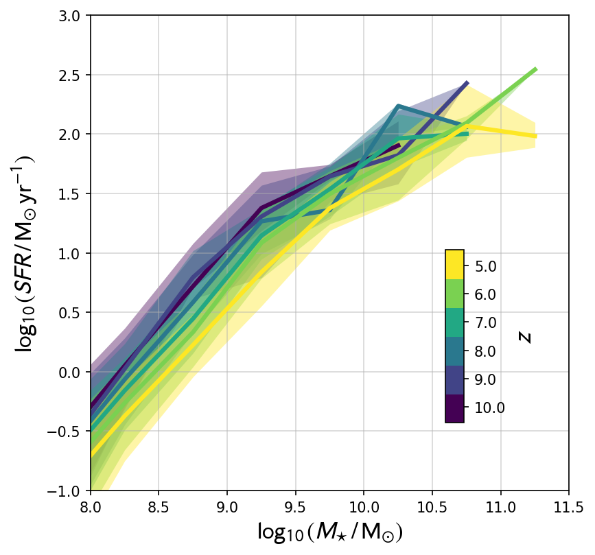
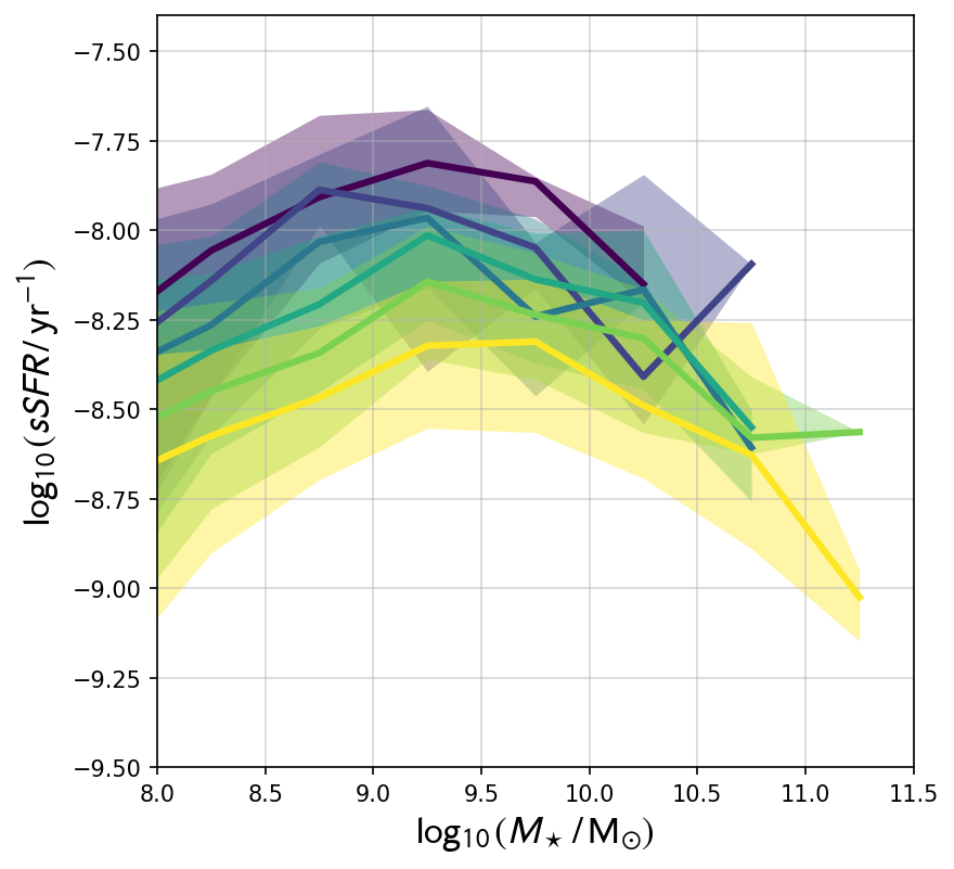
Figure 13: Top: Redshift evolution of the Flares composite star forming sequence. Solid lines show the weighted composite SFS for centrals + satellites, with the 16^th-84^th spread shaded. Bottom: as for the top panel, but showing the specific-star formation rate - stellar mass relation.

The top panel of Figure 13 shows the redshift evolution of the SFS in Flares. In the bottom panel of Figure 13 we also show the specific-star formation rate (sSFR) against $M_{\star}$ relation. To construct the median lines, we weight each galaxy in the sample by the appropriate factor for the overdensity of the resimulation volume, as described in Section 2.4. There is a clear trend of decreasing normalisation with decreasing redshift, approximately $0.5$ dex between $z=10\,-\,5$. There is some noise in the weighted relation at $z=8$ for galaxies with $M_{\star}>10^{9.5}\,M_{\odot}$; we checked, and found that this is due to a small number of galaxies in mean density regions above this mass limit with low SFRs, biasing the normalisation down.

We have not excluded ‘passive’ galaxies from our measurement of the SFS. We present results for the SFS assuming different specific-SFR cuts in Appendix B, though note here that they make negligible difference to the relations at $z\geqslant 5$ for even the most liberal cuts.

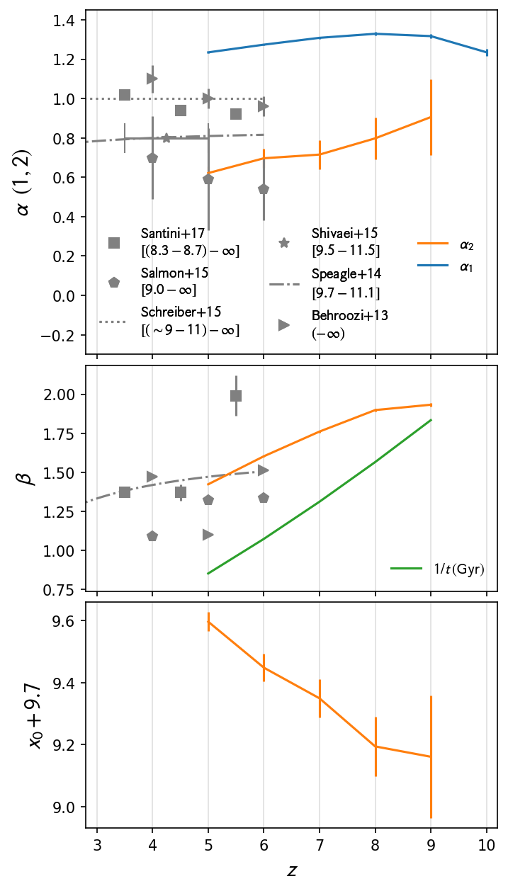
Figure 14: Redshift evolution of the piecewise-linear fit to the SFS. Observational results are plotted where available in grey, from Behroozi et al. (2013); Speagle et al. (2014); Shivaei et al. (2015); Salmon et al. (2015); Schreiber et al. (2015); Santini et al. (2017). The lower- and upper-mass completeness limits for these studies are quoted in the legend. Top: high- and low-mass slope, in orange and blue respectively. Middle: normalisation, $\beta$, in orange. The inverse age of the Universe in Gyr is shown in green; the normalisation approximately follows the same relation, but with a slightly shallower evolution. Bottom: turnover mass in log-solar masses, in orange.

There is a clear turnover in the Flares star-forming sequence at high masses ($\sim\,>\,10^{9.3}\mathrm{M_{\odot}}$). We account for this by fitting a piecewise-linear relation, with an upper- and lower-mass part, for stellar mass re-normalised at $10^{9.7}\mathrm{M_{\odot}}$,

$$\log_{10}\psi=\alpha_{1}\,\mathrm{log_{10}}(M_{\star}\,/\,10^{9.7}\mathrm{M_{\odot}})+\beta_{1}\quad x\leqslant x_{0}$$ (11)

$$\log_{10}\psi=\alpha_{2}\,\mathrm{log_{10}}(M_{\star}\,/\,10^{9.7}\mathrm{M_{\odot}})+\beta_{2}\quad x\geq x_{0}\;,$$ (12)

where $\alpha_{1}$ is the low-mass slope, $\alpha_{2}$ is the high-mass slope, and $x_{0}$ is the turnover mass in log-solar masses. The normalisation at the turnover, $\beta_{0}$, is then given by

$$\beta_{0} =\beta_{2}+\alpha_{2}\,x_{0}$$ (13)

$$=\beta_{1}+\alpha_{1}\,x_{0}\;\;.$$ (14)

We use the scipy implementation of non-linear least squares to perform the fit, combined with a non-parametric bootstrap approach for estimating parameter uncertainties. The bootstrap is implemented as follows: we select, with replacement, 10 000 times from the original data, each resample being the same size as the original data. We then fit each sample independently; parameter estimates are given by the median of the resampled fit distributions, and uncertainties are given as the 1$\sigma$ spread in the distributions (unless otherwise stated). The parameter fits are quoted in Table 5.

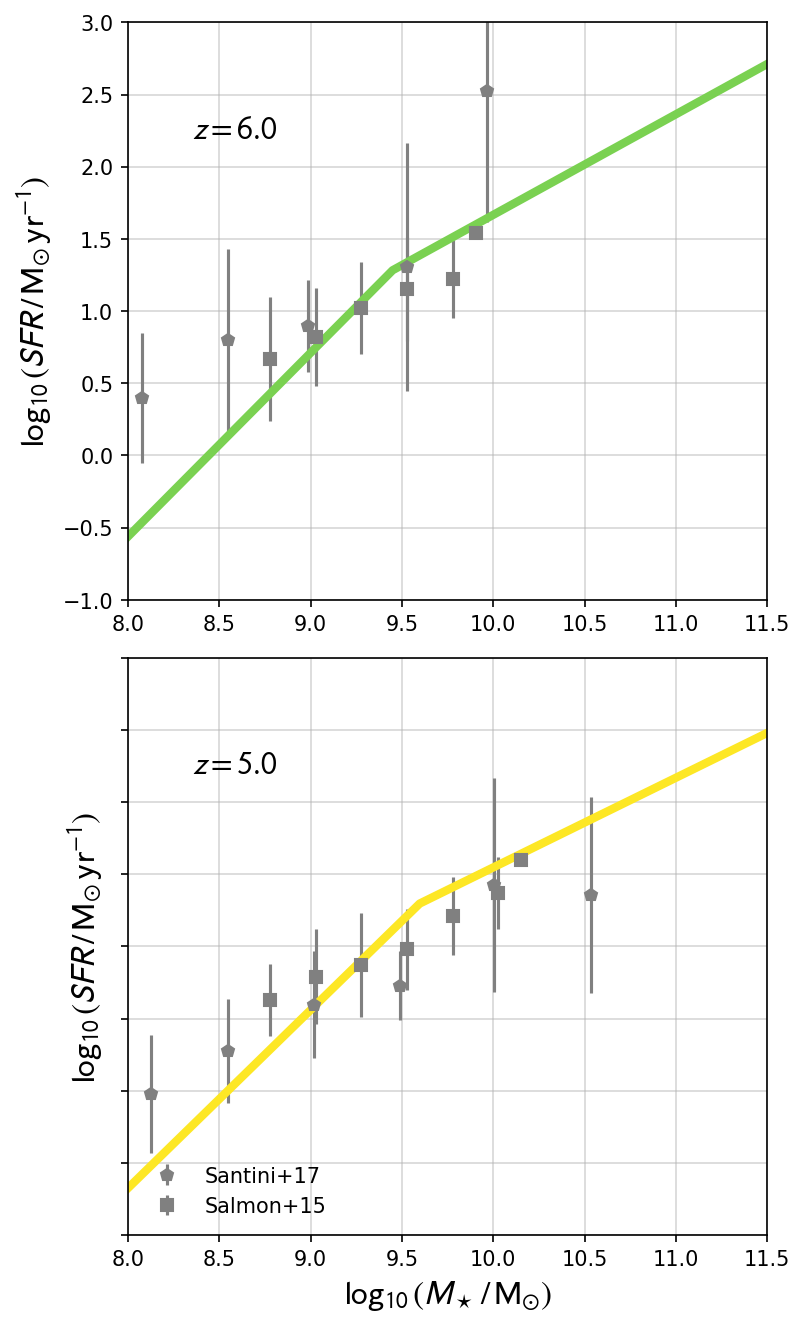
Figure 15: Flares composite SFS at $z=5.0$ and $6.0$ compared to high redshift observational constraints from Santini et al. (2017) and Song et al. (2016).

Figure 14 shows the redshift evolution of each parameter against observational constraints where available. There are few robust observational constraints at $z>6$, so we show constraints down to $z=3$ to provide context to the redshift evolution (Behroozi et al., 2013; Schreiber et al., 2015; Shivaei et al., 2015; Salmon et al., 2015; Santini et al., 2017), including the compilation of pre-2014 measurements from Speagle et al. (2014). These all represent single power-law measurements. For all observations we quote the approximate lower mass completeness limit for the whole fit in the legend. We also show a direct comparison of the fits to binned data from Santini et al. (2017) and Salmon et al. (2015) in Figure 15 at $z=5\,-\,6$.

The normalisation is within the errors of the binned observations at these redshifts. The fitted normalisation $\beta$ is also within the spread of the fitted relations at these redshifts, and continues the apparent increasing normalisation with increasing redshift from $z=3$. We also show the inverse age of the Universe (in Gyr); the fall in SFS normalisation approximately follows the same relation, but slightly shallower.

The slope of the observed relations shows considerable scatter spanning the range $\sim\,0.5-1.1$. We suggest that this is due to the lower-mass limit of these observations (quoted in the legend of Figure 14). Since these studies fit a single power-law, and assume a high lower-mass completeness limit, ($M_{\star}\,/\,M_{\odot}>10^{9.5}$), the measured slope will be biased to shallower slopes. This can also be seen clearly in the binned relations in Figure 15; both Santini et al. (2017) and Song et al. (2016) straddle the turnover mass in Flares. Finally, this can also be seen in the redshift evolution of these studies. The observed slopes of Salmon et al. (2015), Behroozi et al. (2013) and Santini et al. (2017) all show a negative correlation with redshift. The lower-mass completeness limit of these studies also increases with increasing redshift; as it increases, they tend to probe just the high-mass end of the SFS, rather than the steeper low-mass end. This suggests that many high redshift measures of the SFS, where the mass completeness does not extend to very low masses, are only probing the SFS at stellar masses above the turnover, and the measured slopes do not represent a universal relation for all masses.

The turnover mass shows a negative correlation with redshift, increasing from $\sim 10^{9.2}$ to $10^{9.6}\,M_{\star}\,/\,M_{\odot}$ between $z=9-5$. Ceverino et al. (2018) show no turnover in their FirstLight simulation results, but they do not probe above $10^{9.5}$ at $z=6$, which is consistent with where we constrain the turnover. There are unfortunately no observational constraints on the turnover mass at $z>3$. We note that the turnover mass is much lower than that measured in low-$z$ studies ($>10^{10}\,M_{\star}\,/\,M_{\odot}$ at $z\leqslant 3$, Whitaker et al., 2014; Tasca et al., 2015).

3.4.1 Environmental dependence of the SFS

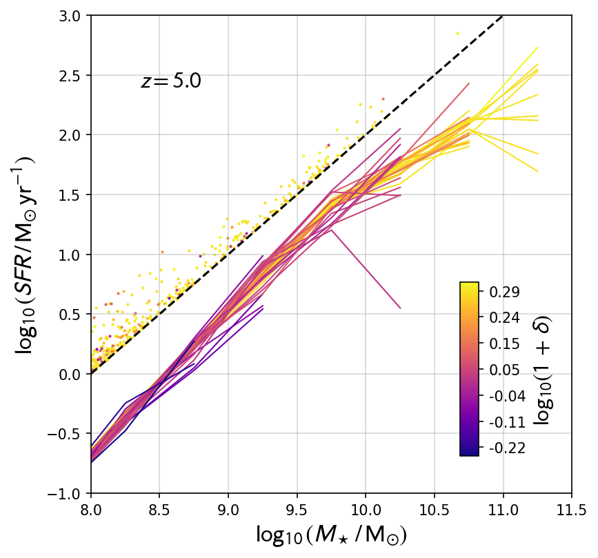
Figure 16: Coloured lines show the SFS for each region at $z=5$, coloured by overdensity. The black dashed line shows a fixed $\mathrm{SSFR}=10^{-8}\;\mathrm{yr^{-1}}$, and points above this show starbursting galaxies, coloured by their host region overdensity.

Figure 16 shows the SFS for each region individually at $z=5$, coloured by overdensity. The highest overdensities reach to higher stellar masses, as expected. However, there is no dependence on overdensity of either the normalisation nor shape of the SFS, and we see this up to $z=10$. Observationally, at $z\sim 2$ there is a similar lack of dependence on environment as measured between protocluster and field regions (Koyama et al., 2013; Koyama et al., 2014; Shimakawa et al., 2017, 2018), though these authors do note some differences in dense subgroups in protocluster candidates (we leave an investigation of the small-scale overdensity dependence of the SFS to future work). However, at $z>5$ Harikane et al. (2019) find a $5\,\times$ enhancement in the SFR (at fixed stellar mass) of Lyman-$\alpha$ emitters in protoclusters compared to the field, though they only probe the low-mass regime ($M_{*}<10^{9}\;M_{\odot}$). It is as yet unclear whether these galaxies represent the main star-forming sequence, or starbursts that lie above it. Harikane et al. (2019) show that dusty star forming galaxies traced in the sub-mm are also spatially correlated with these structures (Geach et al., 2017), and lead to significant enhancements in the cosmic star formation rate density compared to the Madau & Dickinson (2014) relation. In Flares, whilst the normalisation of the SFS at $z=5-6$ is low in the stellar mass regime $M_{*}<10^{9}\;M_{\odot}$ compared to observational constraints (Song et al., 2016; Santini et al., 2017), Figure 16 shows that Flares does produce a number of galaxies with SFRs at least $5\times$ higher than on the main relation, and these are biased to high density regions.

We leave a thorough exploration of the passive and star-bursting galaxy populations in Flares to future work.

4 Conclusions

We have presented the first results from the Flares simulations, resimulations with full hydrodynamics of a range of overdensities during the Epoch of Reionisation (EoR, $z\geqslant 5$) using the Eagle (Schaye et al., 2015) physics. We described our novel weighting procedure that allows the construction of composite distribution functions that mimic extremely large periodic volumes, significantly extending the dynamic range without incurring prohibitively large computational expense. To demonstrate we presented results for the galaxy stellar mass function (GSMF), the star formation rate distribution function (SFRF) and the star-forming sequence (SFS: SFR versus $M_{\star}$). Our findings are as follows:

• The Flares GSMF exhibits a clear double-Schechter shape up to $z=10$. Fits assuming this form show an increasing normalisation, shallower low-mass slope and higher characteristic turnover mass with decreasing redshift. The GSMF is in good agreement with observational constraints at all redshifts up to $z=8$, at which point there is some tension at the knee of the distribution. The normalisation, and to a lesser extent the shape, of the GSMF shows a strong environmental dependence (i.e. bias).

• The SFRF also exhibits a clear double-Schechter shape in the high-SFR regime. As for the GSMF, the normalisation increases and the low-mass slope decreases with decreasing redshift; however the characteristic turnover mass varies only weakly with redshfit. There is a mild tension with observational results, which tend to more closely resemble power law-like distributions. The SFRF shape and normalisation shows a similar environmental dependence to the GSMF.

• The SFS shows no obvious dependence on environment. The low-mass slope is relatively invariant with redshift, whereas the high mass slope decreases with decresing redshift. The characteristic turnover mass increases slowly with decreasing redshift, and the normalisation decreases by about a factor of 3 between redshifts 10 and 5. There is reasonably good agreement with observational constraints at $z=5-6$.

Upcoming space based observatories, such as JWST, Euclid and Roman will provide further probes of the GSMF and SFRF up to $z=10$. The large volumes probed by Euclid and Roman in particular will provide stronger constraints on those extreme galaxies that populate the high-mass / high-SFR tails of each distribution. Our weighting scheme provides a means of testing the latest, high resolution hydrodynamic simulations against such constraints. We will also be able to test the impact of cosmic variance on these large surveys.

Data Availability

The data underlying this article (stellar masses and star formation rates between $z=5-10$) are available at flaresimulations.github.io/data. All of the codes used for the data analysis are public and available at github.com/flaresimulations.

Appendix A Selected regions

Table 4 lists the regions selected from the parent volume for resimulation.

Table 4: Regions selected from the parent volume for resimulation. We provide their positions within the parent volume, their overdensity $\delta$ as defined by Equation 1, their rms overdensity $\sigma$, and weights, $f_{j}$, calculated as per Section 2.4

index	(x, y, z)/(h-1 cMpc)	$\delta$	$\sigma$	$f_{j}$
0	(623.5, 1142.2, 1525.3)	0.970	5.62	0.000027
1	(524.1, 1203.6, 1138.5)	0.918	5.41	0.000196
2	(54.2, 1709.6, 571.1)	0.852	5.12	0.000429
3	(153.6, 1762.0, 531.3)	0.849	5.11	0.000953
4	(39.8, 1686.1, 1850.6)	0.846	5.09	0.000444
5	(847.6, 1444.0, 1062.6)	0.842	5.07	0.000828
6	(1198.2, 135.5, 1375.3)	0.841	5.07	0.000666
7	(1012.0, 1514.4, 1454.8)	0.839	5.06	0.001178
8	(591.0, 359.6, 1610.2)	0.839	5.06	0.000265
9	(746.4, 820.5, 945.2)	0.833	5.03	0.001029
10	(1181.9, 1171.1, 974.1)	0.830	5.02	0.000387
11	(38.0, 670.5, 47.0)	0.829	5.02	0.000719
12	(1989.7, 368.7, 2076.5)	0.828	5.01	0.000668
13	(1659.0, 1306.6, 760.8)	0.824	4.99	0.000488
14	(57.8, 883.7, 2098.2)	0.821	4.98	0.001190
15	(609.0, 2018.6, 115.7)	0.820	4.98	0.000757
16	(122.9, 1124.1, 1304.8)	0.616	4.00	0.003738
17	(1395.2, 415.7, 1575.9)	0.616	4.00	0.004678
18	(128.3, 216.9, 258.4)	0.431	3.00	0.009359
19	(1400.6, 1686.1, 806.0)	0.431	3.00	0.012324
20	(699.4, 1760.2, 1725.9)	0.266	2.00	0.029311
21	(1951.8, 2022.3, 1709.6)	0.266	2.00	0.027954
22	(755.4, 1122.3, 867.5)	0.121	1.00	0.057876
23	(516.9, 325.3, 603.6)	0.121	1.00	0.062009
24	(937.9, 1382.5, 1077.1)	-0.007	0.00	0.074502
25	(1675.3, 1492.8, 1335.5)	-0.007	0.00	0.080377
26	(1270.5, 518.7, 862.0)	-0.121	-1.00	0.063528
27	(242.2, 1881.3, 1624.7)	-0.121	-1.00	0.058231
28	(1454.8, 1720.5, 1608.4)	-0.222	-2.00	0.034467
29	(430.1, 296.4, 359.6)	-0.222	-2.00	0.024216
30	(1733.1, 1097.0, 1060.8)	-0.311	-3.00	0.012087
31	(1821.7, 947.0, 1431.3)	-0.311	-3.00	0.013127
32	(1913.8, 1033.7, 45.2)	-0.066	-0.50	0.064280
33	(2009.6, 2024.1, 1693.4)	-0.066	-0.50	0.066277
34	(339.8, 934.3, 1646.4)	-0.007	0.00	0.076001
35	(1693.4, 914.5, 1977.1)	-0.007	-0.00	0.076486
36	(778.9, 900.0, 1866.8)	0.055	0.50	0.070408
37	(1790.9, 1239.7, 1765.6)	0.055	0.50	0.062451
38	(2078.3, 77.7, 141.0)	-0.479	-5.29	0.002721
39	(818.7, 110.2, 1628.3)	-0.434	-4.61	0.003366

Appendix B The impact of cutting passive galaxies from the star forming sequence

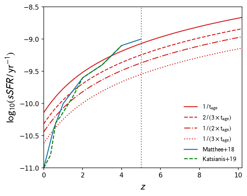
Figure 17: Evolving sSFR cuts for passive galaxies. Cuts used in Katsianis et al. (2019); Matthee & Schaye (2019) shown for comparison.

In Section 3.4 we showed the SFS assuming no cut for passive galaxies. We now briefly explore the impact of applying an evolving cut in specific star formation rate (sSFR), and how this impacts the SFS. We employ an sSFR cut that excludes those galaxies whose current star formation is insufficient to double the mass of the galaxy within twice the current age of the Universe,

$$\mathrm{sSFR}>\frac{1}{2\times t_{\mathrm{age}}}\;\;,$$ (15)

which leads to an evolving threshold for quiescence with redshift, shown in Figure 17. Using this cut, we exclude 979 galaxies at $z=5$ (out of a total of 32824 with stellar masses above $10^{8}\,M_{\odot}$).

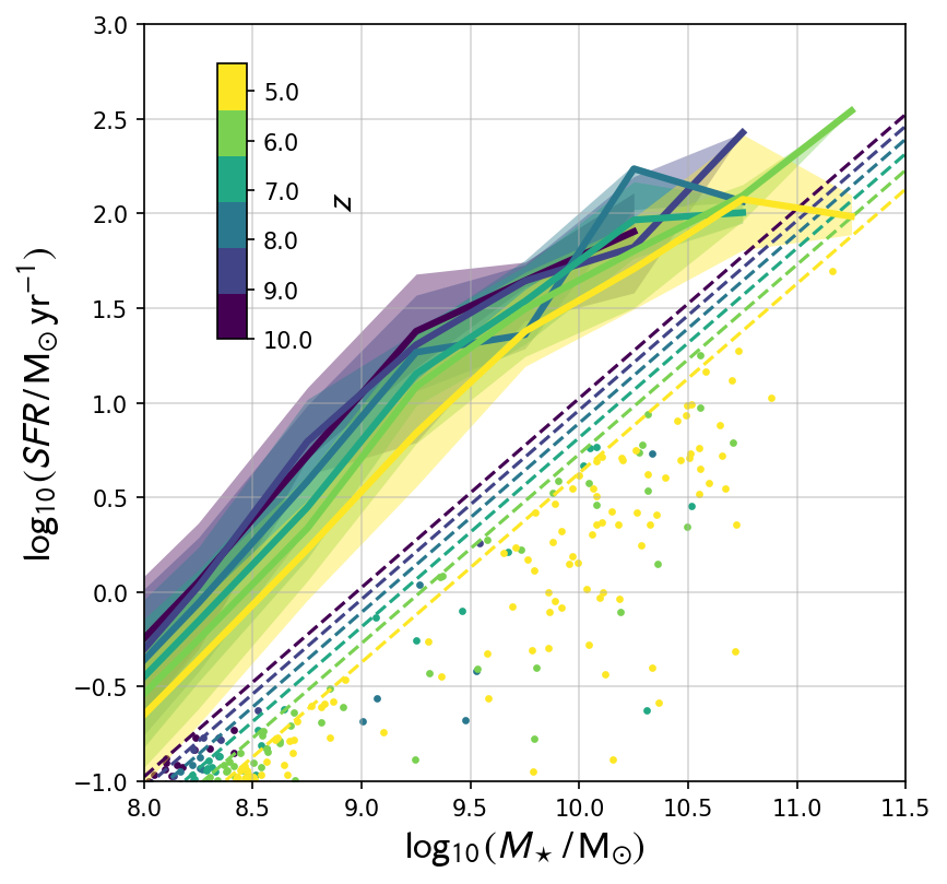
Figure 18: SFS assuming a sSFR cut for passive galaxies. These cuts are shown by the coloured dashed lines at each redshift. Points show individual passive galaxies that satisfy the cut. The relations are essentially identical to those without a passive galaxy cut.

Figure 18 shows the SFS assuming this cut. There is almost no difference between this relation and that shown in Figure 13. We tested using different thresholds (mass multiples of $\times\frac{3}{2}$ and $\times 3$) and found that all our results are insensitive to the multiple of mass chosen. Observations typically use UVJ colour to discriminate quiescent objects (e.g. Whitaker et al., 2011); at $z\sim 2$, this leads to a similar threshold for quiescence as a sSFR cut (Fang et al., 2018).

Appendix C Fitted distribution functions

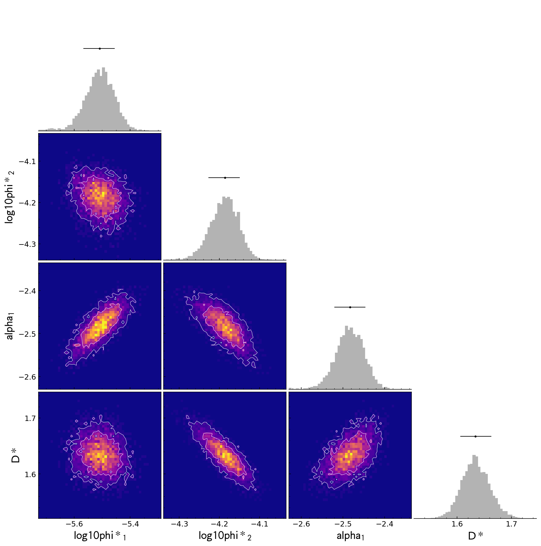
Figure 19: Posteriors from the Galaxy Stellar Mass Function fit at $z=7$. $\alpha_{2}$ is fixed at -1 and is not shown.

Table 6 and 7 show double-Schechter fit parameters to the GSMF and SFRF. We use FitDF, a python module for fitting arbitrary distribution functions using Markov Chain Monte Carlo (MCMC). FitDF is built around the popular emcee package (v3.0, Foreman-Mackey et al., 2013). The code can be found at https://github.com/flaresimulations/fitDF.

A Poisson form of the likelihood is typically used for distribution function analyses in Astronomy due to the relatively small number of observations. Due to our resimulation approach we cannot use this form of the likelihood, since the number counts obtained from the composite approach, scaled to the size of the parent box volume, significantly underestimate the errors. Instead, we use a Gaussian form for the likelihood,

$$\mathrm{log}(\mathcal{L})=-\frac{1}{2}\,\left[\sum_{i}\,\frac{(N_{i,\mathrm{obs}}-N_{i,\mathrm{exp}})^{2}}{\sigma_{i}^{2}}\,+\mathrm{log}(\sigma_{i}^{2})\right]\;\;,$$ (16)

where the subscript $i$ represents the bin of the property being measured, $N_{i,\mathrm{obs}}$ is the inferred number of galaxies using the composite number density multiplied by the parent box volume, $N_{i,\mathrm{exp}}$ is the expected number from the model, and $\sigma_{i}$ is the error estimate. Using this form, $\sigma$ can be explicitly provided from the resimulated number counts, $\sigma_{i}=N_{i,\mathrm{obs}}/\sqrt{n_{i,\mathrm{obs}}}$, where $n_{i,\mathrm{obs}}$ is the number counts in bin $i$ from the resimulations.

We use flat uniform priors in $\mathrm{log_{10}}(D^{*})$, $\alpha_{1}$, $\mathrm{log_{10}}(\phi^{*}_{1})$ and $\mathrm{log_{10}}(\phi^{*}_{2})$. We fix $\alpha_{2}=-1$ by setting a narrow top-hat prior around this value. We run chains of length $10^{4}$, then calculate the autocorrelation time, $\tau$, on these chains (Goodman & Weare, 2010). We use $\tau$ to estimate the burn-in ($\tau\times 4$) and thinning ($\tau/2$) on our chains. Example posteriors for each parameter in a fit to the $z=7$ GSMF are shown as a corner plot in Figure 19.

Table 5 shows the piecewise-fits to the SFS; the fitting procedure is described in Section 3.4.

z	$x_{0}+9.7$	$\alpha_{1}$	$\alpha_{2}$	$\beta$
5	9.60	1.23	0.62	1.42
6	9.45	1.27	0.70	1.60
7	9.35	1.31	0.72	1.76
8	9.20	1.33	0.80	1.90
9	9.16	1.31	0.91	1.93
10	-	1.24	-	-

Table 5: Best fitting two-part piecewise-linear fits to the star-forming sequence.

z	M∗	log10($\phi^{*}_{1}$ /(Mpc-3 dex-1))	log10($\phi^{*}_{2}$ /(Mpc-3 dex-1))	$\alpha_{1}$
10	$9.117_{-0.045}^{+0.041}$	$-6.557_{-0.197}^{+0.188}$	$-4.871_{-0.07}^{+0.065}$	$-3.542_{-0.206}^{+0.193}$
9	$9.488_{-0.044}^{+0.036}$	$-6.372_{-0.112}^{+0.116}$	$-4.832_{-0.057}^{+0.056}$	$-3.07_{-0.077}^{+0.076}$
8	$9.577_{-0.041}^{+0.039}$	$-5.904_{-0.08}^{+0.081}$	$-4.565_{-0.058}^{+0.059}$	$-2.83_{-0.048}^{+0.065}$
7	$9.831_{-0.035}^{+0.039}$	$-5.443_{-0.054}^{+0.051}$	$-4.374_{-0.059}^{+0.052}$	$-2.515_{-0.032}^{+0.03}$
6	$10.089_{-0.035}^{+0.029}$	$-5.057_{-0.047}^{+0.036}$	$-4.156_{-0.046}^{+0.05}$	$-2.293_{-0.023}^{+0.019}$
5	$10.326_{-0.02}^{+0.019}$	$-4.686_{-0.024}^{+0.023}$	$-3.942_{-0.034}^{+0.033}$	$-2.11_{-0.011}^{+0.012}$

Table 6: Best fitting double-Schechter function parameter values for the Galaxy Stellar Mass Function. $\alpha_{2}$ is fixed at $-1$.

z	SFR∗	log10($\phi^{*}_{1}$ /(Mpc-3 dex-1))	log10($\phi^{*}_{2}$ /(Mpc-3 dex-1))	$\alpha_{1}$
5	$1.402_{-0.067}^{+0.049}$	$-6.525_{-0.123}^{+0.142}$	$-5.022_{-0.069}^{+0.07}$	$-2.978_{-0.074}^{+0.071}$
5	$1.359_{-0.044}^{+0.036}$	$-5.941_{-0.093}^{+0.093}$	$-4.645_{-0.058}^{+0.058}$	$-2.772_{-0.06}^{+0.064}$
5	$1.433_{-0.028}^{+0.032}$	$-5.639_{-0.066}^{+0.059}$	$-4.431_{-0.058}^{+0.049}$	$-2.62_{-0.045}^{+0.051}$
5	$1.633_{-0.027}^{+0.03}$	$-5.509_{-0.057}^{+0.052}$	$-4.186_{-0.04}^{+0.036}$	$-2.482_{-0.038}^{+0.036}$
5	$1.684_{-0.015}^{+0.015}$	$-5.059_{-0.039}^{+0.041}$	$-3.907_{-0.026}^{+0.024}$	$-2.307_{-0.025}^{+0.026}$
5	$1.755_{-0.012}^{+0.011}$	$-4.68_{-0.033}^{+0.033}$	$-3.644_{-0.02}^{+0.02}$	$-2.139_{-0.019}^{+0.02}$

Table 7: Best fitting double-Schechter function parameter values for the Star Formation Rate distribution function. $\alpha_{2}$ is fixed at $-1$.

References

- Atek et al. (2018) Atek H., Richard J., Kneib J.-P., Schaerer D., 2018, MNRAS, 479, 5184
- Bahé et al. (2016) Bahé Y. M., et al., 2016, MNRAS, 456, 1115
- Bahé et al. (2017) Bahé Y. M., et al., 2017, MNRAS, 470, 4186
- Baldry et al. (2008) Baldry I. K., Glazebrook K., Driver S. P., 2008, MNRAS, 388, 945
- Barnes et al. (2017a) Barnes D. J., Kay S. T., Henson M. A., McCarthy I. G., Schaye J., Jenkins A., 2017a, MNRAS, 465, 213
- Barnes et al. (2017b) Barnes D. J., et al., 2017b, MNRAS, 471, 1088
- Barrow et al. (2017) Barrow K. S. S., Wise J. H., Norman M. L., O’Shea B. W., Xu H., 2017, MNRAS, 469, 4863
- Baugh (2006) Baugh C. M., 2006, Rep. Prog. Phys., 69, 3101
- Beckwith et al. (2006) Beckwith S. V. W., et al., 2006, AJ, 132, 1729
- Behroozi & Silk (2018) Behroozi P., Silk J., 2018, Monthly Notices of the Royal Astronomical Society, 477, 5382
- Behroozi et al. (2013) Behroozi P. S., Wechsler R. H., Conroy C., 2013, ApJ, 770, 57
- Benitez-Llambay (2015) Benitez-Llambay A., 2015, py-sphviewer: Py-SPHViewer v1.0.0, doi:10.5281/zenodo.21703, http://dx.doi.org/10.5281/zenodo.21703
- Benson (2010) Benson A. J., 2010, Phys. Rep., 495, 33
- Bhatawdekar et al. (2019) Bhatawdekar R., Conselice C. J., Margalef-Bentabol B., Duncan K., 2019, Monthly Notices of the Royal Astronomical Society, 486, 3805
- Bouwens et al. (2015) Bouwens R. J., et al., 2015, ApJ, 803, 34
- Bower et al. (2017) Bower R. G., Schaye J., Frenk C. S., Theuns T., Schaller M., Crain R. A., McAlpine S., 2017, MNRAS, 465, 32
- Brinchmann et al. (2004) Brinchmann J., Charlot S., White S. D. M., Tremonti C., Kauffmann G., Heckman T., Brinkmann J., 2004, MNRAS, 351, 1151
- Bromm & Yoshida (2011) Bromm V., Yoshida N., 2011, Annu. Rev. Astron. Astrophys., 49, 373
- Castellano et al. (2016) Castellano M., et al., 2016, ApJ, 823, L40
- Ceverino et al. (2018) Ceverino D., Klessen R. S., Glover S. C. O., 2018, Monthly Notices of the Royal Astronomical Society, 480, 4842
- Chabrier (2003) Chabrier G., 2003, PASP, 115, 763
- Chiang et al. (2013) Chiang Y.-K., Overzier R., Gebhardt K., 2013, ApJ, 779, 127
- Chiang et al. (2017) Chiang Y.-K., Overzier R. A., Gebhardt K., Henriques B., 2017, ApJL, 844, L23
- Clay et al. (2015) Clay S., Thomas P., Wilkins S., Henriques B., 2015, MNRAS, 451, 2692
- Cooray et al. (2019) Cooray A., et al., 2019, Conference Proceedings, 51, 48
- Crain et al. (2009) Crain R. A., et al., 2009, MNRAS, 399, 1773
- Crain et al. (2015) Crain R. A., et al., 2015, MNRAS, 450, 1937
- Crain et al. (2017) Crain R. A., et al., 2017, MNRAS, 464, 4204
- Cullen & Dehnen (2010) Cullen L., Dehnen W., 2010, Mon Not R Astron Soc, 408, 669
- Daddi et al. (2007) Daddi E., et al., 2007, ApJ, 670, 156
- Davé et al. (2019) Davé R., Anglés-Alcázar D., Narayanan D., Li Q., Rafieferantsoa M. H., Appleby S., 2019, MNRAS, 486, 2827
- Davis et al. (1985) Davis M., Efstathiou G., Frenk C. S., White S. D. M., 1985, ApJ, 292, 371
- Dayal & Ferrara (2018) Dayal P., Ferrara A., 2018, Physics Reports, 780, 1
- Di Matteo et al. (2017) Di Matteo T., Croft R. A. C., Feng Y., Waters D., Wilkins S., 2017, MNRAS, 467, 4243
- Dubois et al. (2014) Dubois Y., et al., 2014, MNRAS, 444, 1453
- Duncan et al. (2014) Duncan K., et al., 2014, MNRAS, 444, 2960
- Durier & Dalla Vecchia (2012) Durier F., Dalla Vecchia C., 2012, Mon Not R Astron Soc, 419, 465
- Fang et al. (2018) Fang J. J., et al., 2018, ApJ, 858, 100
- Feng et al. (2015) Feng Y., Di Matteo T., Croft R., Tenneti A., Bird S., Battaglia N., Wilkins S., 2015, ApJ, 808, L17
- Feng et al. (2016) Feng Y., Di-Matteo T., Croft R. A., Bird S., Battaglia N., Wilkins S., 2016, MNRAS, 455, 2778
- Finlator et al. (2018) Finlator K., Keating L., Oppenheimer B. D., Davé R., Zackrisson E., 2018, preprint, 1805, arXiv:1805.00099
- Foreman-Mackey et al. (2013) Foreman-Mackey D., Hogg D. W., Lang D., Goodman J., 2013, Publications of the Astronomical Society of the Pacific, 125, 306
- Furlong et al. (2015) Furlong M., et al., 2015, MNRAS, 450, 4486
- Furlong et al. (2017) Furlong M., et al., 2017, MNRAS, 465, 722
- Gardner et al. (2006) Gardner J. P., et al., 2006, Space Science Reviews, 123, 485
- Geach et al. (2017) Geach J. E., et al., 2017, MNRAS, 465, 1789
- Genel et al. (2014) Genel S., et al., 2014, Monthly Notices of the Royal Astronomical Society, 445, 175
- Gnedin (2014) Gnedin N. Y., 2014, ApJ, 793, 29
- Gonzalez et al. (2011) Gonzalez V., Labbe I., Bouwens R., Illingworth G., Franx M., Kriek M., 2011, ApJ, 735, L34
- Goodman & Weare (2010) Goodman J., Weare J., 2010, Communications in Applied Mathematics and Computational Science, 5, 65
- Grogin et al. (2011) Grogin N. A., et al., 2011, ApJS, 197, 35
- Harikane et al. (2019) Harikane Y., et al., 2019, The Astrophysical Journal, 883, 142
- Henriques et al. (2015) Henriques B. M. B., White S. D. M., Thomas P. A., Angulo R., Guo Q., Lemson G., Springel V., Overzier R., 2015, MNRAS, 451, 2663
- Henriques et al. (2020) Henriques B. M. B., Yates R. M., Fu J., Guo Q., Kauffmann G., Srisawat C., Thomas P. A., White S. D. M., 2020, MNRAS, 491, 5795
- Hopkins (2013) Hopkins P. F., 2013, Mon Not R Astron Soc, 428, 2840
- Hunter (2007) Hunter J. D., 2007, Computing in Science & Engineering, 9, 90
- Ilbert et al. (2013) Ilbert O., et al., 2013, A&A, 556, A55
- Ishigaki et al. (2018) Ishigaki M., Kawamata R., Ouchi M., Oguri M., Shimasaku K., Ono Y., 2018, ApJ, 854, 73
- Jaacks et al. (2019) Jaacks J., Finkelstein S. L., Bromm V., 2019, MNRAS, 488, 2202
- Katsianis et al. (2017) Katsianis A., et al., 2017, MNRAS, 472, 919
- Katsianis et al. (2019) Katsianis A., et al., 2019, ApJ, 879, 11
- Katz & White (1993) Katz N., White S. D. M., 1993, ApJ, 412, 455
- Katz et al. (2017) Katz H., Kimm T., Sijacki D., Haehnelt M. G., 2017, MNRAS, 468, 4831
- Kelvin et al. (2014) Kelvin L. S., et al., 2014, MNRAS, 444, 1647
- Kennicutt Jr & Evans II (2012) Kennicutt Jr R. C., Evans II N. J., 2012, ARAA, 50, 531
- Khandai et al. (2015) Khandai N., Di Matteo T., Croft R., Wilkins S. M., Feng Y., Tucker E., DeGraf C., Liu M.-S., 2015, MNRAS, 450, 1349
- Koekemoer et al. (2011) Koekemoer A. M., et al., 2011, ApJS, 197, 36
- Koyama et al. (2013) Koyama Y., et al., 2013, MNRAS, 434, 423
- Koyama et al. (2014) Koyama Y., Kodama T., Tadaki K.-i., Hayashi M., Tanaka I., Shimakawa R., 2014, ApJ, 789, 18
- Lacey et al. (2016) Lacey C. G., et al., 2016, MNRAS, 462, 3854
- Lagos et al. (2015) Lagos C. d. P., et al., 2015, MNRAS, 452, 3815
- Lagos et al. (2019) Lagos C. d. P., et al., 2019, MNRAS, 489, 4196
- Laureijs et al. (2011) Laureijs R., et al., 2011, arXiv e-prints, 1110, arXiv:1110.3193
- Lee et al. (2015) Lee N., et al., 2015, ApJ, 801, 80
- Leja et al. (2015) Leja J., Dokkum P. G. v., Franx M., Whitaker K. E., 2015, ApJ, 798, 115
- Livermore et al. (2017) Livermore R. C., Finkelstein S. L., Lotz J. M., 2017, ApJ, 835, 113
- Lovell et al. (2018) Lovell C. C., Thomas P. A., Wilkins S. M., 2018, MNRAS, 474, 4612
- Lower et al. (2020) Lower S., Narayanan D., Leja J., Johnson B. D., Conroy C., Davé R., 2020, arXiv:2006.03599 [astro-ph]
- Ma et al. (2018) Ma X., et al., 2018, MNRAS, 478, 1694
- Madau & Dickinson (2014) Madau P., Dickinson M., 2014, ARAA, 52, 415
- Matteo et al. (2012) Matteo T. D., Khandai N., DeGraf C., Feng Y., Croft R. A. C., Lopez J., Springel V., 2012, ApJ, 745, L29
- Matthee & Schaye (2019) Matthee J., Schaye J., 2019, MNRAS, 484, 915
- McAlpine et al. (2016) McAlpine S., et al., 2016, A&C, 15, 72
- McCracken et al. (2012) McCracken H. J., et al., 2012, A&A, 544, A156
- Moffett et al. (2016) Moffett A. J., et al., 2016, MNRAS, 457, 1308
- Nelson et al. (2017) Nelson D., et al., 2017, preprint, 1707, arXiv:1707.03395
- Noeske et al. (2007) Noeske K. G., et al., 2007, ApJL, 660, L43
- O’Shea et al. (2015) O’Shea B. W., Wise J. H., Xu H., Norman M. L., 2015, ApJ, 807, L12
- Ocvirk et al. (2016) Ocvirk P., et al., 2016, MNRAS, 463, 1462
- Pforr et al. (2012) Pforr J., Maraston C., Tonini C., 2012, MNRAS, 422, 3285
- Pforr et al. (2013) Pforr J., Maraston C., Tonini C., 2013, MNRAS, 435, 1389
- Pillepich et al. (2017) Pillepich A., et al., 2017, arXiv:1707.03406 [astro-ph]
- Planck Collaboration et al. (2014) Planck Collaboration et al., 2014, A&A, 571, A1
- Poole et al. (2016) Poole G. B., Angel P. W., Mutch S. J., Power C., Duffy A. R., Geil P. M., Mesinger A., Wyithe S. B., 2016, MNRAS, 459, 3025
- Price (2008) Price D. J., 2008, Journal of Computational Physics, 227, 10040
- Robitaille et al. (2013) Robitaille T. P., et al., 2013, A&A, 558, A33
- Rodrigues et al. (2017) Rodrigues L. F. S., Vernon I., Bower R. G., 2017, MNRAS, 466, 2418
- Rosdahl et al. (2018) Rosdahl J., et al., 2018, MNRAS
- Salim & Lee (2012) Salim S., Lee J. C., 2012, The Astrophysical Journal, 758, 134
- Salmon et al. (2015) Salmon B., et al., 2015, ApJ, 799, 183
- Santini et al. (2009) Santini P., et al., 2009, A&A, 504, 751
- Santini et al. (2017) Santini P., et al., 2017, ApJ, 847, 76
- Schaller et al. (2015) Schaller M., Dalla Vecchia C., Schaye J., Bower R. G., Theuns T., Crain R. A., Furlong M., McCarthy I. G., 2015, Mon Not R Astron Soc, 454, 2277
- Schaye et al. (2010) Schaye J., et al., 2010, Monthly Notices of the Royal Astronomical Society, 402, 1536
- Schaye et al. (2015) Schaye J., et al., 2015, MNRAS, 446, 521
- Schechter (1976) Schechter P., 1976, ApJ, 203, 297
- Schreiber et al. (2015) Schreiber C., et al., 2015, A&A, 575, A74
- Shimakawa et al. (2017) Shimakawa R., et al., 2017, MNRAS
- Shimakawa et al. (2018) Shimakawa R., et al., 2018, MNRAS, 481, 5630
- Shivaei et al. (2015) Shivaei I., et al., 2015, ApJ, 815, 98
- Simpson et al. (2014) Simpson J. M., et al., 2014, ApJ, 788, 125
- Smit et al. (2012) Smit R., Bouwens R. J., Franx M., Illingworth G. D., Labbé I., Oesch P. A., Dokkum P. G. v., 2012, ApJ, 756, 14
- Smith & Hayward (2015) Smith D. J. B., Hayward C. C., 2015, MNRAS, 453, 1597
- Smith et al. (2017) Smith A., Bromm V., Loeb A., 2017, A&G, 58, 3.22
- Somerville & Davé (2015) Somerville R. S., Davé R., 2015, ARAA, 53, 51
- Somerville et al. (2015) Somerville R. S., Popping G., Trager S. C., 2015, MNRAS, 453, 4337
- Song et al. (2016) Song M., et al., 2016, ApJ, 825, 5
- Speagle et al. (2014) Speagle J. S., Steinhardt C. L., Capak P. L., Silverman J. D., 2014, ApJS, 214, 15
- Spergel et al. (2015) Spergel D., et al., 2015, arXiv:1503.03757 [astro-ph]
- Springel et al. (2001) Springel V., White S. D. M., Tormen G., Kauffmann G., 2001, MNRAS, 328, 726
- Springel et al. (2005) Springel V., et al., 2005, Nature, 435, 629
- Stark (2016) Stark D. P., 2016, Annu. Rev. Astron. Astrophys., 54, 761
- Stefanon et al. (2017) Stefanon M., Bouwens R. J., Labbé I., Muzzin A., Marchesini D., Oesch P., Gonzalez V., 2017, ApJ, 843, 36
- Tasca et al. (2015) Tasca L. a. M., et al., 2015, A&A, 581, A54
- Tomczak et al. (2016) Tomczak A. R., et al., 2016, ApJ, 817, 118
- Tormen et al. (1997) Tormen G., Bouchet F. R., White S. D. M., 1997, MNRAS, 286, 865
- Trayford et al. (2015) Trayford J. W., et al., 2015, MNRAS, 452, 2879
- Trayford et al. (2017) Trayford J. W., et al., 2017, MNRAS, 470, 771
- Tremmel et al. (2016) Tremmel M., Karcher M., Governato F., Volonteri M., Quinn T., Pontzen A., Anderson L., 2016, arXiv:1607.02151 [astro-ph]
- Vijayan et al. (2019) Vijayan A. P., Clay S. J., Thomas P. A., Yates R. M., Wilkins S. M., Henriques B. M., 2019, MNRAS, 489, 4072
- Virtanen et al. (2020) Virtanen P., et al., 2020, Nature Methods, 17, 261
- Vogelsberger et al. (2014) Vogelsberger M., et al., 2014, MNRAS, 444, 1518
- Warren et al. (2007) Warren S. J., et al., 2007, MNRAS, 375, 213
- Waters et al. (2016) Waters D., Di Matteo T., Feng Y., Wilkins S. M., Croft R. A. C., 2016, MNRAS, 463, 3520
- Wendland (1995) Wendland H., 1995, Adv Comput Math, 4, 389
- Whitaker et al. (2011) Whitaker K. E., et al., 2011, ApJ, 735, 86
- Whitaker et al. (2014) Whitaker K. E., et al., 2014, ApJ, 795, 104
- Wilkins et al. (2011) Wilkins S. M., Bunker A. J., Lorenzoni S., Caruana J., 2011, MNRAS, 411, 23
- Wilkins et al. (2016a) Wilkins S. M., Feng Y., Di Matteo T., Croft R., Stanway E. R., Bouwens R. J., Thomas P., 2016a, MNRAS, 458, L6
- Wilkins et al. (2016b) Wilkins S. M., Feng Y., Di-Matteo T., Croft R., Stanway E. R., Bunker A., Waters D., Lovell C., 2016b, MNRAS, 460, 3170
- Wilkins et al. (2017) Wilkins S. M., Feng Y., Di Matteo T., Croft R., Lovell C. C., Waters D., 2017, MNRAS, 469, 2517
- Wilkins et al. (2018) Wilkins S. M., Feng Y., Di Matteo T., Croft R., Lovell C. C., Thomas P., 2018, MNRAS, 473, 5363
- Wilkins et al. (2020) Wilkins S. M., et al., 2020, MNRAS
- Yoshida (2019) Yoshida N., 2019, Proc Jpn Acad, 95, 17
- Yung et al. (2019a) Yung L. Y. A., Somerville R. S., Finkelstein S. L., Popping G., Davé R., 2019a, MNRAS, 483, 2983
- Yung et al. (2019b) Yung L. Y. A., Somerville R. S., Popping G., Finkelstein S. L., Ferguson H. C., Davé R., 2019b, MNRAS, 490, 2855
- Zaroubi (2013) Zaroubi S., 2013, in Wiklind T., Mobasher B., Bromm V., eds, Astrophysics and Space Science Library, The First Galaxies: Theoretical Predictions and Observational Clues. Springer, Berlin, Heidelberg, pp 45–101, doi:10.1007/978-3-642-32362-1_2, https://doi.org/10.1007/978-3-642-32362-1_2