DIV=10,\KOMAoptionsnumbers=noenddot \KOMAoptionstwoside=semi, twocolumn=false, headinclude=false,footinclude=false,mpinclude=false,headlines=2.1,headsepline=true,footsepline=false,cleardoublepage=empty \KOMAoptionsparskip=relative, \KOMAoptions\KOMAoptions\KOMAoptionsbibliography=totoc \KOMAoptions\KOMAoptions\KOMAoptions ection]section \setkomafontsection \setkomafontsubsection \setkomafontsubsubsection \setkomafontparagraph \setkomafontpageheadfoot
Sampling Rates for -Synthesis
[2em]2em
Maximilian März§, Claire Boyer∗, Jonas Kahn†, Pierre Weiss‡
Affiliations: §Technische Universität Berlin; ∗LPSM, Sorbonne Université, ENS Paris; †Université de Toulouse; ‡ITAV, CNRS, Université de Toulouse
E-Mail of corresponding author: §maerz@math.tu-berlin.de
Abstract. This work investigates the problem of signal recovery from undersampled noisy sub-Gaussian measurements under the assumption of a synthesis-based sparsity model. Solving the -synthesis basis pursuit allows for a simultaneous estimation of a coefficient representation as well as the sought-for signal. However, due to linear dependencies within redundant dictionary atoms it might be impossible to identify a specific representation vector, although the actual signal is still successfully recovered. The present manuscript studies both estimation problems from a non-uniform, signal-dependent perspective. By utilizing recent results on the convex geometry of linear inverse problems, the sampling rates describing the phase transitions of each formulation are identified. In both cases, they are given by the conic Gaussian mean width of an -descent cone that is linearly transformed by the dictionary. In general, this expression does not allow a simple calculation by following the polarity-based approach commonly found in the literature. Hence, two upper bounds involving the sparsity of coefficient representations are provided: The first one is based on a local condition number and the second one on a geometric analysis that makes use of the thinness of high-dimensional polyhedral cones with not too many generators. It is furthermore revealed that both recovery problems can differ dramatically with respect to robustness to measurement noise – a fact that seems to have gone unnoticed in most of the related literature. All insights are carefully undermined by numerical simulations.
Key words. Compressed sensing, inverse problems, sparse representations, redundant dictionaries, non-uniform recovery, Gaussian mean width, circumangle.
1 Introduction
In the last two decades, the methodology of compressive sensing promoted the use of sparsity based methods for many signal processing tasks. Following the seminal works of Candès, Donoho, Romberg and Tao [CRT06, CT06, Don06], a vast amount of research has extended the understanding, how additional structure can be exploited for solving ill-posed inverse problems. The classical setup in this area considers a non-adaptive, linear measurement model, which reads as follows:
The goal of compressive sensing is to solve this inverse problem by reconstructing an approximation of the signal from its indirect measurements . Remarkably, even if , this task can be achieved by incorporating additional information during the reconstruction process. Most classical compressive sensing works directly assume that is -sparse, i.e., that at most entries of are nonzero or in symbols . However, this assumption is hardly satisfied in any real-world application. Nevertheless, many signals allow for sparse representations using specific transforms, such as Gabor dictionaries, wavelet systems or data-adaptive representations, which are inferred from a given set of training samples. Such a model is referred to as synthesis formulation, since it assumes that there exists a matrix and a low-complexity representation such that can be “synthesized” as
| (1.2) |
Following the standard terminology of the field, the matrix will be henceforth refered to as dictionary and its columns as dictionary atoms. It can be expected that the coefficient vector is dominated by just a few large entries, provided that allows to capture the signal’s inherent structure reasonably well.
The synthesis formulation of compressive sensing exploits such a representation model, for instance, by employing greedy-based reconstruction algorithms or by utilizing the sparsity-promoting effect of the -norm. In this work, we will consider the following convex program, which we refer to as synthesis basis pursuit for coefficient recovery:
| () |
Under suitable assumptions, one might hope that solutions of this minimization program approximate reasonably well. Indeed, if , the formulation () turns into the classical basis pursuit. It allows to recover any -sparse vector with overwhelming probability, if additionally follows a suitable random distribution and [FR13].
In many practical and theoretical situations, it turns out that using redundant dictionaries, i.e., choosing , is beneficial. For instance, the stationary wavelet transform overcomes the lack of translation invariance and learned dictionaries typically infer a larger set of convolutional filters, which are adapted to a particular data distribution. If does not form a basis, representations as in (1.2) are not necessarily unique anymore. Hence, it is not to be expected that a specific representation can be identified by solving (). However, in many situations of interest, the representation vector itself is irrelevant and a recovery of the actual signal is of primary interest. Thus, one rather cares about the synthesis basis pursuit for signal recovery, which amounts to solving
| () |
In the noiseless case (i.e., when and ), it might be the case that , but there is still hope that . In other words, although solving () might fail in identifying a specific coefficient representation, it is still possible that the actual signal is successfully recovered by a subsequent synthesis with .
1.1 What This Paper Is About
The goal of this work is to broaden the understanding of the conditions that guarantee coefficient and signal recovery by solving () and (), respectively. To that end, we believe that addressing the following, non-exhaustive list of questions will be of particular importance:
-
(Q1)
Under which circumstances does coefficient and signal recovery differ, i.e., when is it impossible to reconstruct a specific coefficient representation although the signal itself might still be identified?
-
(Q2)
If possible, how many measurements are required to reconstruct a specific coefficient representation? Analogously, how many measurements are required to recover the associated signal?
-
(Q3)
In case that coefficients and signals can both be identified, are there still differences between the two formulations, for instance with respect to robustness to measurement noise?
Set out to find answers to these questions, we first restrict ourselves to the following sub-Gaussian measurement model, which will be considered in this work unless stated otherwise:
This model has been established as a somewhat classical benchmark setup in the context of compressive sensing. It allows us to follow the methodology initiated in [RV07, MPT07] and extended in [Sto09, CRPW12, Tro15, ALMT14]. In a nutshell, the aim is to determine the sampling rate of a convex program (i.e., the number of required measurements for successful recovery) by calculating the so-called Gaussian mean width.
We now briefly outline our work and summarize its main contributions:
-
(C1)
A cornerstone of our analysis is formed by the set of minimal -representers of :
() Independently of Model 1.1, Section 3.1 reveals that if , exact recovery of via () is equivalent to perfect recovery of by solving (). Furthermore, exact recovery of a coefficient vector by () is only possible, if is the unique minimal -representer of , i.e., if .
-
(C2)
In Section 3.2 and Section 3.3, it will be shown that the sampling rate of both formulations can be expressed by the squared conic mean width , where denotes the descent cone of the -norm at any (see Section 2 for a brief summary of the general recovery framework and definitions of these notions). This observation holds unconditionally true in the case of signal recovery by (). For coefficient recovery the additional assumption that is a singleton needs to be satisfied.
-
(C2’)
While forms a precise description of the sampling rate, it is a quantity that is hard to analyze and compute, in general. Therefore, an important goal of our work is to derive more informative upper bounds for this expression. First, under the assumption that is a singleton, we show a condition number bound that relates to the classical complexity , where (see Section 4.1).
The second upper bound of Section 4.2 is central to our work. It is based on a geometric analysis that makes use of generic arguments from high-dimensional convex geometry. In comparison to the first bound, it is more general since we do not assume that is a singleton. Hence, it particularly addresses the recovery of signals, without requiring the identification of a coefficient representation. The resulting upper bound on the conic mean width relies on the thinness of high-dimensional polyhedral cones with not exponentially many generators. We believe that such an argument might be of general interest beyond its application to the synthesis formulation of compressive sensing. Again, is related to the sparsity of a minimal -representation and a further geometrical parameter (referred to as circumangle) that measures the narrowness of the associated cone.
- (C3)
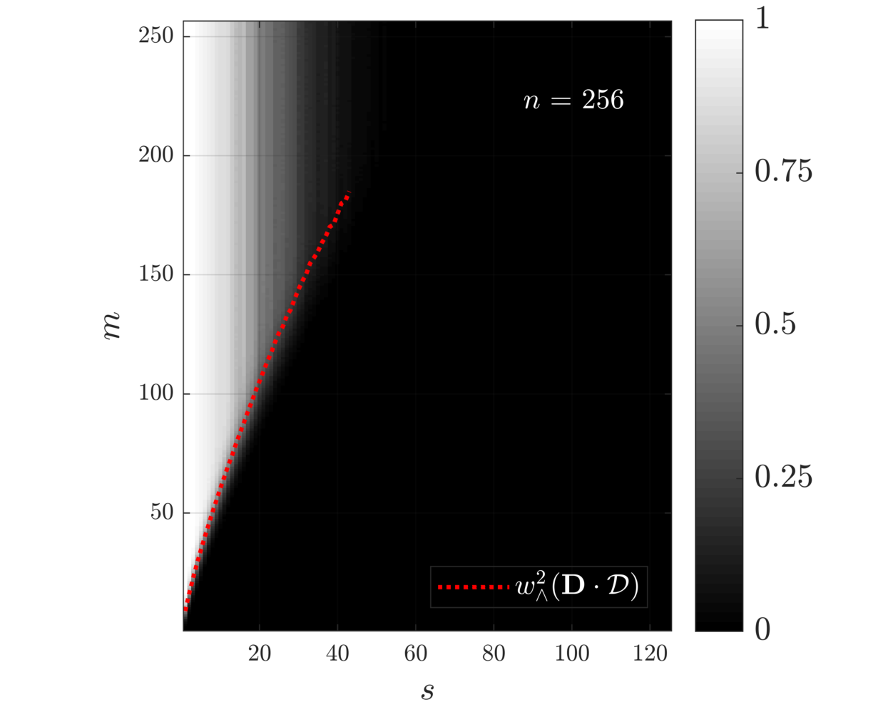
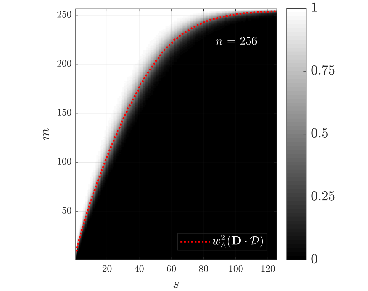
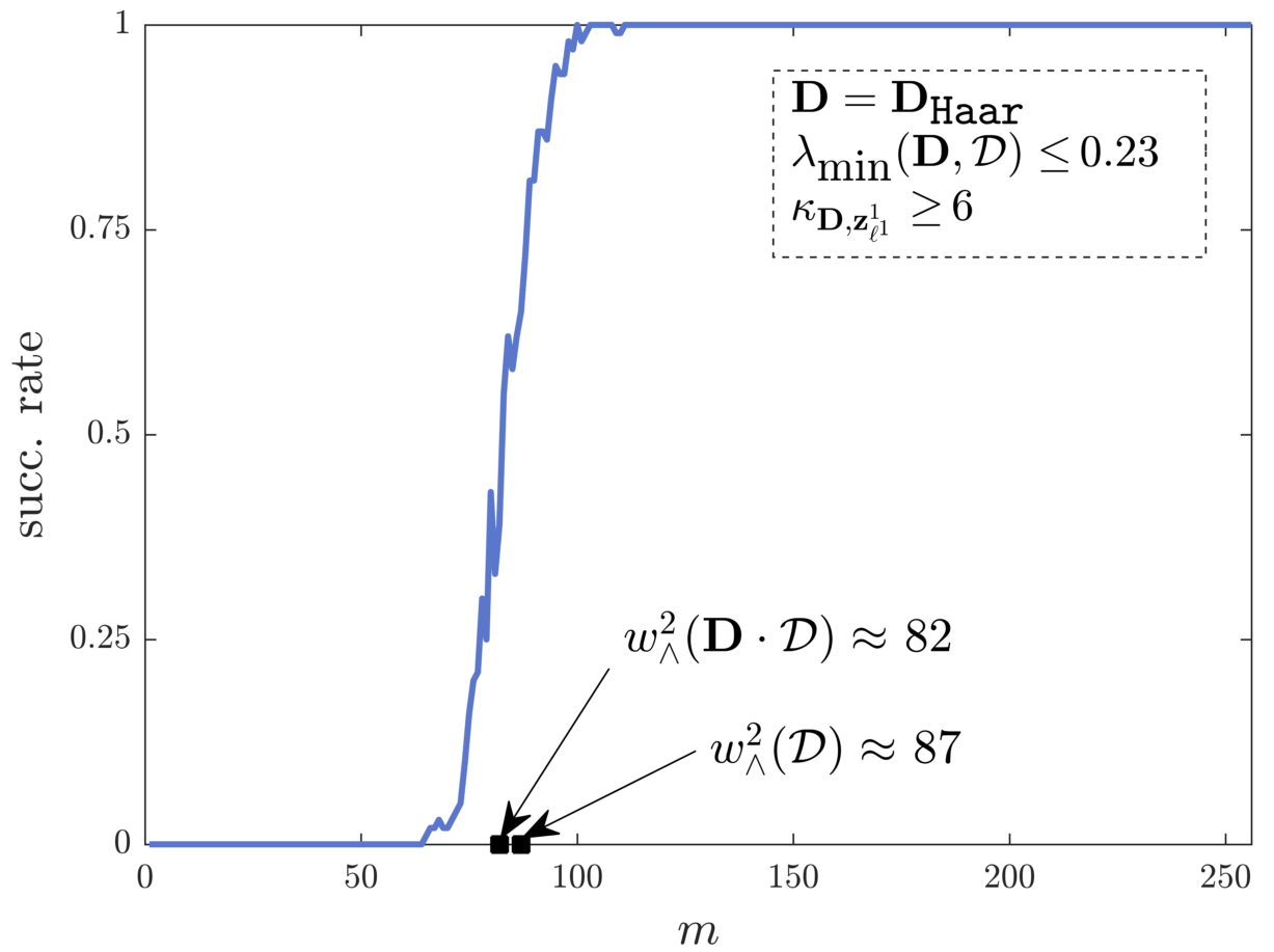
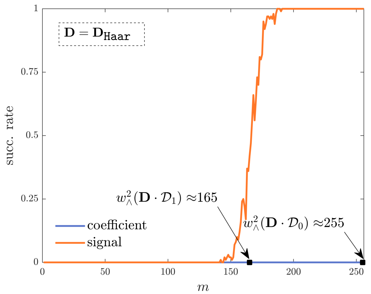
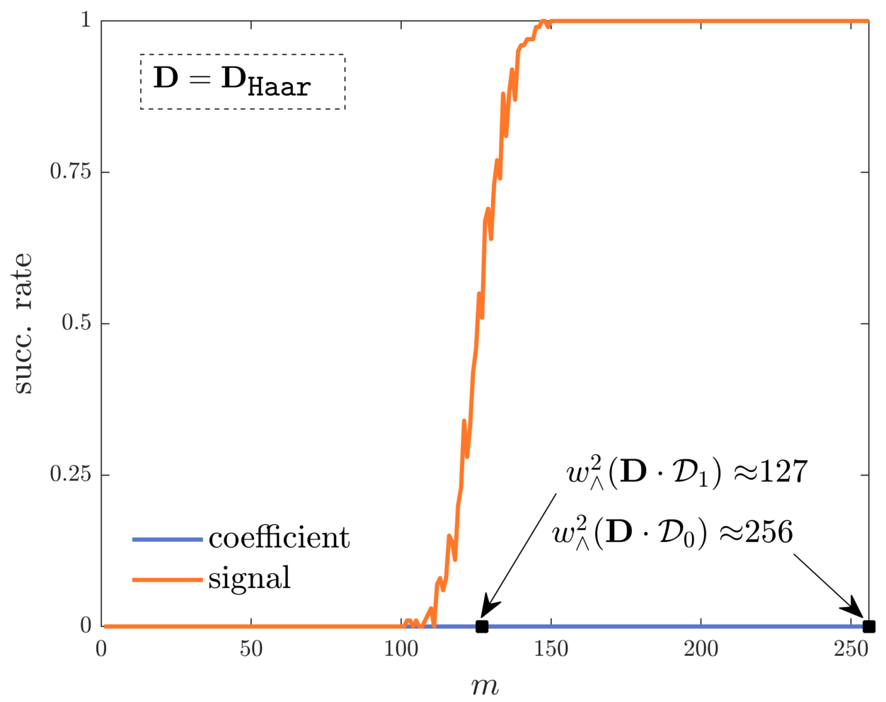
All our findings are underpinned by extensive numerical experiments; see Section 5. As a first “teaser” we refer the reader to Figure 1, which displays two phase transition plots and our sampling rates for a redundant Haar wavelet system .
1.2 Related Literature
In the following, we first briefly discuss some historical references that are of general interest for -norm minimization, sparse representations in redundant dictionaries and compressive sensing. Subsequently, we focus on the existing literature on the synthesis formulation in more depth.
1.2.1 Some Historical Landmarks
The idea of promoting sparsity in discrete or continuous dictionaries by -norm minimization can be traced back to the works of Beurling [Beu38] and Krein [Kre38]. Motivated by questions in Banach space geometry, first theorems establishing sparsity of solutions of related minimization problems can be found in the 1940’s [Zuh48]. In his PhD-thesis of 1965, Logan utilized -minimization for sparse frequency estimation [Log65] and in the 1970’s it was employed for solving deconvolution problems in geophysics [CM73, TBM79]. Of particular importance became the so-called Rudin-Osher-Fatemi-model [ROF92], which pioneered the use of total variation minimization for image processing tasks.
The field of sparse representations arose with the development of (greedy) algorithms for finding expansions in redundant dictionaries such as time-frequency systems [MZ93, PRK93]. Subsequently, the work [CDS98] triggered notable interest in achieving this task by solving the basis pursuit (); see for instance [EB02, DH01, DE03]. A special emphasis was thereby given to unions of orthogonal bases [EB02, GN03, CR06]. Next to the classical concepts of coherence and spark, which are uniform across all -sparse signals, also the non-uniform notions of dual certificates and exact recovery conditions were progressively introduced [Fuc04, Tro04, Fuc05, Tro06].
Under the notion of compressive sensing, Candès, Romberg and Tao [CRT06, CRT06a] and Donoho [Don06] first proposed to capitalize on randomized models in the basis pursuit. In these works, the structured dictionary is replaced by a random matrix , which follows for instance Model 1.1. Such a design allows to overcome severe shortcomings of previous results, in particular the quadratic/square root-bottleneck; see next subsection or [FR13, Chapter 5.4]. Indeed, under such a randomness assumption, it can be shown that any -sparse vector can be recovered with overwhelming probability if the number of measurements obeys . These seminal works can furthermore be acknowledged for highlighting the remarkable potential of sparsity-based methods for many signal recovery tasks.
1.2.2 Results on the Synthesis Formulation of Compressed Sensing
An important insight on solving the inverse problem of Model 1 by means of redundant dictionaries was provided by Elad, Milanfar and Rubinstein [EMR07]. Therein, the authors compare two different formulations: The synthesis basis pursuit () and an alternative formulation, which is referred to as -analysis basis pursuit:
| (1.4) |
The analysis operator is thereby chosen in such a way that the coefficient vector is of low-complexity. It turns out that the latter formulation and the program () are only equivalent if (or ) forms a basis. In particular for redundant choices of and , the geometry of both formulations departs significantly from each other. While the synthesis variant appears to be more natural from a historical perspective, its analysis-based counterpart gained considerable attention in the past years [CENR11, NDEG13, GNEGD14, KNW15, KR15, KRZ15]. Recently, the non-uniform approach of [GKM20] revealed that the measure of “low-complexity” in the analysis model goes beyond pure sparsity of . Instead, a novel sampling-rate bound was proposed that is based on a generalized notion of sparsity, taking the support and the coherence structure of the underlying analysis operator into account.
The earliest reference that deals with the synthesis formulation for the recovery of coefficient vectors appears to be by Rauhut, Schnass and Vandergheynst [RSV08]. Therein, the formulation () is studied under a randomized measurement model. The main result roughly reads as follows: Assume that the dictionary satisfies a restricted isometry property (RIP) with sparsity level . If the random matrix follows Model 1.1 and , then the composition will also satisfy an RIP with sparsity level with high probability. This property then implies stable and robust recovery of all -sparse coefficient vectors by solving (). The assumption that satisfies an RIP is crucial for the previous result. It can be for instance achieved if the dictionary is sufficiently incoherent, i.e., if it satisfies
| (1.5) |
However, as the authors of [RSV08] point out, such a coherence-based estimate is rather crude and suffers from the so-called square-root bottleneck: The Welch bound [FR13, Theorem 5.7] reveals that condition (1.5) can only be satisfied for mild sparsity values .
In [CWW14], Chen, Wang and Wang study conditions for signal recovery via a dictionary-based null space property (NSP): For a given dictionary , a matrix is said to satisfy the -NSP of order , if for any index set with and any , there exists , such that . It can be shown that this condition is necessary and sufficient for the uniform recovery of all signals with via (). Note that the -NSP is in general weaker than requiring that satisfies the standard NSP. This means that the previous result is addressing signal recovery without necessarily requiring coefficient recovery. However, the authors then show that under the additional assumption that is of full spark (i.e., every columns of are linearly independent), both conditions are in fact equivalent. Hence, in this case, signal and coefficient recovery are also equivalent. In the recent work [CCL19], this serves as a motivation to study coefficient recovery by analyzing how many measurements are required in order to guarantee that has an NSP. To that end, a result is provided that is conceptually similar to [RSV08], however, it reduces the assumptions on . Instead of requiring that satisfies an RIP, the authors operate under the weaker assumption that satisfies an NSP. The main result essentially reads as follows: Under a sub-Gaussian measurement setup similar to Model 1.1 and under the assumption that satisfies an NSP of order , a number of measurements guarantees that also satisfies an NSP. This condition then allows for robust recovery of all -sparse coefficient vectors by solving ().
To the best of our knowledge, the only work that provides a bound on the required number of measurement for signal recovery (without necessarily requiring coefficient recovery) is the tutorial [Ver15, Theorem 7.1]: Assume that , and that for an -sparse representation . For a Gaussian measurement matrix , Vershynin establishes the following recovery bound in expectation:
| (1.6) |
where is a constant and is a solution of (). Note that we have slightly adapted the statement of [Ver15, Theorem 7.1] for a better match with our setup. Due to the first summand on the right hand side, the previous error bound is suboptimal, cf. Theorem 3.8. In particular, it does not guarantee exact recovery from noiseless measurements. We emphasize that parts of our work are inspired by Vershynin, who also studies the gauge of the set in [Ver15].
We conclude by mentioning a few more works in the literature on synthesis based compressed sensing that appear to be of less relevance for this work. The influential paper [CRPW12] studies signal recovery via atomic minimization, however, it does not provide specific insights when redundant dictionaries are used. In [DNW13], a (theoretical) CoSaMP algorithm is adapted to the recovery of signals with sparse representations in redundant dictionaries. Based on the -RIP [CENR11] and on a connection to the analyis formulation with so-called optimal dual frames, [LLMLY12] derives a theorem concerning signal recoery. Finally, [SF09] provides numerical experiments, which empirically compare the analysis and the synthesis formulation.
1.2.3 The Gap that We Intend to Fill
In order to obtain statements that are uniform across all -sparse signals, most existing results assume that the dictionary satisfies strong assumptions, e.g., incoherent atoms, an NSP or an RIP [RSV08, CWW14, CCL19]. Such notions are well established and allow for appealing results that often resemble known principles of compressive sensing. However, in many situations of interest, these assumptions are too restrictive. In particular, redundant representation systems (such as Gabor systems, wavelets, curvelets, …) or data-adaptive dictionaries do not satisfy any such property. Their atoms are typically highly coherent and share many linear dependencies. We aim to address this issue by following a local, non-uniform approach, which avoids strong assumptions on the dictionary. We believe that such a signal-dependent refinement is crucial for redundant representation systems, cf. [GKM20].
Similarly, it is occasionally argued that distinguishing signal and coefficient recovery is of minor importance, cf. [CCL19]. This is justified by the observation that exact recovery of coefficients and signals is equivalent if is in general position. However, due to the linear dependencies in many structured representation systems, such an argumentation is often not valid. Indeed, simple numerical experiments with popular dictionaries reveal that signal recovery can be frequently observed without reconstructing a specific coefficient representation, see Figure 1 and Section 5. Hence, we believe that it is important to study both formulations and to identify under which conditions coefficient recovery might be expected, see (C1) above.
To the best of our knowledge, this is the first work that provides a precise description of the phase transition behavior of both formulations, see (C2). While the identified conic mean width of a linearly transformed set is a rather implicit quantity, it constitutes an important step towards the understanding of -synthesis. By deriving more explicit upper bounds on the sampling rate, coefficient sparsity is identified as an important factor. However, additional properties that account for the local geometry are also taken into account, see (C2’).
Last but not least, we establish that both formulations behave differently with respect to robustness to measurement noise, see (C3). To the best of our knowledge, this aspect has gone unnoticed in the literature so far, although it might have dramatic implications on the reconstruction quality of coefficient representations.
1.3 Notation
For the convenience of the reader, we have collected the most important and frequently used objects in Table 1.
Throughout this manuscript we will use the following notation and conventions: for an integer we set . If , we let denote the complement of in . Vectors and matrices are symbolized by lower- and uppercase bold letters, respectively. Let . For an index set , we let the vector denote the restriction to the components indexed by . The support of is defined by the set of its non-zero entries and the sparsity of is . For , denotes the -norm on . The associated unit ball is given by and the Euclidean unit sphere is . The -th standard basis vector of is refered to as and denotes the identity matrix. Furthermore, let denote the conic hull of a set . If is a linear subspace, the associated orthogonal projection onto is given by . Then, we have , where is the orthogonal complement of . The letter is usually reserved for a (generic) constant, whose value could change from time to time. We refer to as a numerical constant if its value does not depend on any other involved parameter. If an (in-)equality holds true up to a numerical constant , we sometimes write instead of . For a matrix we let denote its spectral norm. For a set , and we set and . Lastly, the term orthonormal basis is abbreviated by ONB.
2 A Primer on the Convex Geometry of Linear Inverse Problems
In this section, we give a brief introduction to a well-established methodology that addresses the recovery of structured signals from independent linear random measurements. This summary mainly serves the purpose of introducing the required technical notions for our subsequent analysis of the -synthesis formulation. It is inspired by [CRPW12, Tro15, ALMT14] and we refer the interested reader to these works for a more detailed discussion of the presented material.
2.1 Minimum Conic Singular Value
Assume that Model 1 is satisfied. For a robust recovery of from its linear, noisy measurements , we consider the generalized basis pursuit
| () |
where is a convex function that is supposed to reflect the “low complexity” of the signal . Hence, the previous minimization problem searches for the most structured signal that is still consistent with the given measurements .
The recovery performance of () can be understood by a fairly standard geometric analysis. It seeks to understand the geometric interplay of the structure-promoting functional and the measurement matrix in a neighborhood of the signal vector . To that end, we first introduce the following notions of descent cones and minimum conic singular values.
Definition 2.1 (Descent cone)
Let be a convex function and let . The descent set of at is given by
| (2.1) |
and the corresponding descent cone is defined by .
The notion of minimum conic singular values describes the behavior of a matrix when it is restricted to a cone .
Definition 2.2 (Minimum conic singular value)
Consider a matrix and a cone . The minimum conic singular value of with respect to the cone is defined by
| (2.2) |
The following result characterizes exact recoverability of the signal and provides a deterministic error bound for the solutions to (). The statement is an adapted version of Proposition 2.1 and Proposition 2.2 in [CRPW12]; see also Proposition 2.6 in [Tro15].
Proposition 2.3 (A deterministic error bound for ())
Assume that and follow Model 1 and let be a convex function. Then the following holds true:
2.2 Conic Mean Width
While Proposition 2.3 provides an elegant analysis of the solutions to the optimization problem (), it can be difficult to apply. The notion of a minimum conic singular value is related to the concept of co-positivity [HS10b] and its computation is known to be an NP-hard task for general matrices and cones [MK87, HS10b].
However, when is chosen at random, sharp estimates can be obtained by exploring a connection to the statistical dimension or Gaussian mean width. These geometric parameters stem from geometric functional analysis and convex geometry (e.g., see [Gor85, Gor88, GM04, Mil85]), but they also show up in Talagrand’s -functional in stochastic processes [Tal14], or under the name of Gaussian complexity in statistical learning theory [BM02]. Their benefits for compressive sensing have first been exploited in [RV07, MPT07]. More important for our work is their use in the more recent line of research [Sto09, CRPW12, ALMT14, Tro15], which aims for non-uniform signal recovery statements.
Definition 2.4
Let be a set.
-
(a)
The (global) mean width of is defined as
(2.4) where is a standard Gaussian random vector.
-
(b)
The conic mean width of is given by
(2.5)
We refer to as the conic mean width of at .
The next theorem is known as Gordon’s Escape Through a Mesh and dates back to [Gor88]. The version presented here follows from [LMPV17].
Theorem 2.5 (Theorem 3 in [LMPV17])
Assume that satisfies the assumption in Model 1.1 and let be a set. Then there exists a numerical constant such that, for every , we have
| (2.6) |
with probability at least . If , we have .
Thus, a straightforward combination the error bound in (2.3) and the estimate in (2.6) for the set reveals that robust recovery via () is possible if the number of sub-Gaussian measurements obeys
| (2.7) |
In the case of Gaussian measurements, it is known that this bound yields a tight description of the so-called phase transition of (). Indeed, for a convex cone it can be shown that with high probability when , where denotes a numerical constant. Applying this statement to the descent cone reveals that exact recovery of by solving () fails with high probability when
| (2.8) |
Hence, exact signal recovery by solving () obeys a sharp phase transition at Gaussian measurements. We refer to [ALMT14] and [Tro15, Remark 3.4] for more details on this matter and conclude our discussion by the following summary:
3 Coefficient and Signal Recovery
Our study of the synthesis formulation in this section is based on the differentiation between coefficient and signal recovery. First, we introduce the set of minimal -representers in Section 3.1 and discuss its importance for the relationship between both formulations. Section 3.2 is then dedicated to the fact that signal recovery via () can be cast as an instance of atomic norm minimization, in which the gauge of the synthesis defining polytope is minimized. Finally, in Section 3.3, we derive two non-uniform recovery theorems that determine the sampling rates of robust coefficient and signal recovery, respectively.
3.1 Recovery and Minimal -Representers
In this section, we discuss how the uniqueness of a minimal -representer impacts coefficient and signal recovery.
Definition 3.1 (Minimal -representers)
The set of minimal -representers of a signal with respect to a dictionary is defined by
| () |
In general, may not be a singleton. Indeed, a coefficient vector can only be the unique minimal -representer of the associated signal , if the set of atoms is linearly independent [FR13, Theorem 3.1]. However, many dictionaries of practical interest possess linear dependent and coherent atoms. Hence, typical notions that would certify uniqueness for all signals with sparse representations in (e.g., the NSP [FR13, Theorem 4.5]) are not expected to hold for such dictionaries.
The following simple lemma shows that exact coefficient recovery by solving () requires to be a singleton. Otherwise, it is impossible to recover a specific coefficient representation, while a retrieval of the signal by () might still be possible.
Lemma 3.2
Assume that and follow Model 1 with . Let be a dictionary such that .
A short proof of the previous result is given in Appendix A.1. Thus, under the assumption that has a unique minimal -representer, exact coefficient recovery by () and signal recovery by () are equivalent.
3.2 Signal Recovery and the Convex Gauge
The literature on compressive sensing predominantly focuses on a recovery of coefficient representations. However, if the goal is to recover the associated signal, this approach may be insufficient for structured dictionaries, as argued previously. In this section, we express the initial optimization problem over the coefficient domain () as a minimization problem over the signal space. The -ball in the coefficient domain is thereby mapped to the convex body , which is referred to as synthesis defining polytope in [EMR07]. The formulation () can be equivalently expressed as a constrained minimization of its corresponding convex gauge.
Definition 3.3 (Convex gauge)
Let be a closed convex set that contains the origin. The gauge of (also referred to as Minkowski functional) is defined as
For a symmetric set (i.e., ) the gauge defines a semi-norm on , which becomes a norm if is additionally bounded.
Lemma 3.4
Assume that and follow Model 1 and let be a dictionary. Then we have:
| (3.1) |
A short proof for his equivalence is given in Appendix A.2. Under the heading of atomic norm minimization, problems of the form (3.1) were previously considered in greater generality in [CRPW12]: Given a collection of atoms , Chandrasekaran et al. study the geometry of signal recovery based on minimizing the associated gauge in (3.1). It turns out that many popular methods such as classical -, or nuclear norm-minimization can be cast in such a form, e.g., by choosing as the set of one-sparse unit-norm vectors, or the set of rank-one matrices with unit-Euclidean-norm. Note that in the considered case of signal recovery via (), one would choose the atoms to obtain . With this reformulation it is evident that dictionary atoms that are convex combinations of the remaining atoms in can be removed without altering [EMR07, Corollary 1].
For some specific problem instances novel sampling rate bounds are derived in [CRPW12]. Although this work plays a key role for the foundation of our work, we wish to emphasize that no explicit insights or bounds are derived in the case of signal recovery with dictionaries. In particular, the connection between () and () has not been studied.
With regard to the recovery framework of Section 2.1, it is of interest to determine the descent cone of the functional at . The following lemma shows how this cone is related to descent cones of the -norm in the coefficient space.
Lemma 3.5
Let be a dictionary and let . For any we have
The proof is given in Appendix A.3.
3.3 Sampling Rates for Signal and Coefficient Recovery
The purpose of this section is to determine the sampling rates for robust coefficient and signal recovery from sub-Gaussian measurements.
Coefficient recovery
With Lemma 3.2 in mind, studying coefficient recovery is meaningful only if the signal has a unique minimal -representer with respect to . Proposition 2.3 implies that this condition can be equivalently expressed by
| (3.2) |
Equipped with this assumption, we now state our main theorem regarding the recovery of coefficient vectors via ().
Theorem 3.6 (Coefficient recovery)
Assume that and follow Model 1, where is drawn according to the sub-Gaussian Model 1.1 with sub-Gaussian norm . Let be a dictionary and be a coefficient vector for the signal , such that
Then there exists a numerical constant such that for every , the following holds true with probability at least : If the number of measurements obeys
| (3.3) |
then any solution to the program () satisfies
| (3.4) |
If , then .
A proof is given in Appendix A.4. Before turning towards signal recovery, let us highlight a few observations regarding the previous theorem.
Remark 3.7
-
(a)
Note that Theorem 3.6 does not assume anything on the dictionary and the coefficient representation , except for , which is a necessary condition for the theorem to hold true. As pointed out above, it reflects that is a unique -representer of with respect to , i.e., that is the unique solution to (). In general, verifying this property is involved (cf. the discussion in Section 2.2) and forms a trail of research on its own, e.g., see [Mal09, Chapter 12] or [CK13, Chapter 9]. In this regard, we think that an important contribution of Theorem 3.6 is that it allows to isolate the minimum prerequisite of a unique -representer in from the actual task of compressive coefficient recovery.
-
(b)
Equation (3.3) identifies as the essential component of the sampling rate for coefficient recovery by (). Indeed, the proof reveals (in combination with the discussion subsequent to Theorem 2.5) that is a tight description of the required number of noiseless Gaussian measurements for exact recovery.
-
(c)
Lastly, the error bound (3.4) shows that coefficient recovery is robust to measurement noise, provided that ; cf. the numerical experiments in Section 5, which confirm this observation. However, we note that this bound might not be tight, in general (cf. the intermediate inequality (A.5) in the proof, which is not necessarily sharp).
Signal recovery
Considering signal recovery by (), a combination of the gauge formulation (3.1), its description of the descent cone in Lemma 3.5, and Theorem 2.5 directly yields the next result.
Theorem 3.8 (Signal recovery)
Let us discuss the previous result in view of its counterpart for coefficient recovery, Theorem 3.6.
Remark 3.9
-
(a)
Similarly as for coefficient recovery, (3.5) identifies as the main quantity of the sampling rate for signal recovery by (). An important difference is that the set minimal of -representers is not required to be a singleton: The descent cone in the signal space may be evaluated at any possible and the resulting sampling rate for signal recovery does not depend on this choice.
-
(b)
In the case of noiseless Gaussian measurements, the number is a tight description of the phase transition of signal recovery, cf. the discussion subsequent to Theorem 2.5.
-
(c)
While the sampling rates for coefficient and signal recovery are similar, the error bounds of the two theorems differ. The inequality (3.6) does not involve the minimal conic singular value as in Theorem 3.6. This suggests the following noteworthy consequence: In the case of simultaneous coefficient and signal recovery, the robustness to noise of () and () might still be different. Indeed, while a reconstruction of is independent of the value of – in fact, even 0 is allowed–, the error with respect to is directly influenced by it. We emphasize that the bound (3.6) cannot be retrieved from the analysis conducted for coefficient recovery. Indeed, the estimate (3.4) of Theorem 3.6 only implies that
(3.7) which is worse than (3.6), in general.
While the bound (3.5) is accurate for an exact recovery from noiseless measurements, it can be improved when an approximate recovery of is already sufficient. This is reflected by the following proposition on stable recovery, which is an adaptation of a result in [GKM20]; see Appendix A.5 for a proof. Note that such an argumentation does not allow for a similar statement about stable coefficient recovery, due to the product in ().
Proposition 3.10 (Stable signal recovery)
The previous result extends Theorem 3.8 by an intuitive trade-off regarding stable signal recovery: By allowing for a lower recovery precision , the number of required measurements can be significantly lowered in comparison to in (3.5). Indeed, (3.8) searches for surrogate representations of in that yield a minimal sampling rate. Note that the original coefficient vector is not required to be a minimal -representer of with respect to . Thus, Proposition 3.10 enables to trade off the required number of measurements against the desired recovery accuracy. The factor is an additional oversampling parameter that may assist in balancing out this trade-off.
We emphasize that this approach to stability is centered around a Euclidean approximation in the signal domain . This is in stark contrast to a stability theory in the coefficient domain, which is typically based on an approximation of compressible vectors by ordinary best -term approximations. We refer to Section 2.4 and 6.1 in [GKM20] as well as Section 2.4 in [GMS20] for more details on the presented approach to stable recovery and related results in the literature.
Remark 3.11
The normalization condition in (3.8) can be discarded at the expense of a slightly worse error bound. Under the same conditions as in Proposition 3.10, we can also derive the following result. Set and let
For every and
the inequality
| (3.11) |
holds true with probability larger than for some constant depending only on the distribution of . For instance, letting with as an oversampling factor, the latter bound essentially becomes:
We conclude this section by an illustration of stable recovery in two simple examples.
Example 3.12
-
(a)
Assume that and let denote a fully populated vector, which is without loss of generality assumed to be positive and nonincreasing. Standard results on the computation of the conic mean width (see for instance [Tro15, Example 4.3]) stipulate that . Hence, it is impossible to exactly recover from noiseless compressive measurements. However, if we are satisfied with an approximate recovery of , we can set the precision for instance to , where denotes the -error of the best -term approximation to . Then, the surrogate vector defined as for and for , satisfies . A straightforward calculation shows that , which eventually leads to . Furthermore, a computation of the conic mean width yields that . Hence, Proposition 3.10 shows that () allows for the reconstruction of an approximation from noiseless sub-Gaussian measurements that satisfies . A comparison with [FR13, Theorem 4.22 and Section 11.1] shows that such a stability result is essentially optimal.
-
(b)
Let us provide another simple result highlighting the important difference between signal and coefficient recovery. Consider a dictionary consisting of a convolution with a low pass filter , i.e., for any , . The problem () then becomes a deconvolution problem and it could be turned to a super-resolution problem by considering non integer shifts of the kernel. In this setting, it is well known [CF14] that coefficients of the form are hard to recover by solving () since . There is a minimum separation distance to respect to guarantee the recovery of sparse spikes with arbitrary signs. We can however use the result (3.11) by setting . In that case, we obtain by picking . Hence, we can recover an -approximation of with a few measurements.
4 Upper Bounds on the Conic Gaussian Width
The previous results identify the conic mean width as the key quantity that controls coefficient and signal recovery by -synthesis. However, this expression does not convey an immediate understanding without further simplification. While tight and informative upper bounds are available for simple dictionaries such as orthogonal matrices, the situation becomes significantly more involved for general, possibly redundant transforms. Indeed, note that the polar cone of is given by . The appearance of the preimage hinders the application of the standard approach based on polarity; see for instance [ALMT14, Recipe 4.1].
Hence, the goal of this section is to provide two upper bounds for that are more accessible and intuitive: Section 4.1 is based on a local conditioning argument, and addresses recovery when a unique minimal -representer exists. The second bound of Section 4.2 follows a geometric analysis that explores the thinness of high-dimensional polyhedral cones with not too many generators. This approach possesses a broader scope and plays a central role in our work.
4.1 A Condition Number Bound
In this section, we aim at “pulling” the dictionary “out of” the expression , in order to make use of the fact that is well understood. We begin by introducing the following notation of a local condition number.
Definition 4.1 (Local condition number)
Let be a dictionary and let be closed convex cone. Then, we define the local condition number of with respect to by
| (4.1) |
with the convention if . We also use the notation , which we refer to as local condition number of at with respect to the -norm.
Before the previous quantity will be used to simplify , we first comment on the origin of its name and give an intuitive interpretation of its meaning in the following remark.
Remark 4.2
-
(a)
First, recall that the classical, generalized condition number of a matrix is defined as the ratio of the largest and the smallest nonzero singular value. Hence, referring to as a local condition number is motivated by the fact that it can also be written as
(4.2) where is the largest singular value of .
-
(b)
Furthermore, note that acts as a local measure for the conditioning of at with respect to the -norm. It quantifies how robustly can be recovered as the minimal -representer of : Consider the perturbation , where with . Thus, in the signal domain we obtain . Proposition 2.3 then yields that any solution of the program
(4.3) satisfies
(4.4) which shows that can be seen as a measure for the stability of with respect to -minimization with .
The following proposition provides a generic upper bound for the conic mean width of a linearly transformed cone.
Proposition 4.3
Let denote a closed convex cone. For any dictionary , we have
| (4.5) |
Proof.
See Appendix B. ∎
Note that for sparse coefficient vectors the quantity is well understood and has been frequently calculated in the literature, see for instance [Tro15, Example 4.3]. It turns out that it can be bounded from above by
| (4.6) |
where . Hence, we directly obtain the following corollary.
Corollary 4.4
We have assumed to be a unique minimal -representer since otherwise the previous statement becomes meaningless due to . Thus, the condition number bound of Corollary 4.4 foremost addresses coefficient recovery via (), as well as a reconstruction of signals with unique minimal -representers in by (). In both cases, sub-Gaussian measurements are sufficient (recall that the two formulations might nevertheless differ with respect to robustness to measurement noise). Hence, the results of this section identify the following three decisive factors for successful recovery:
-
(i)
The uniqueness of as the minimal -representer of ;
-
(ii)
The complexity of with respect to -norm, which is measured by , or by its sparsity ;
-
(iii)
The quantity , which resembles a local measure for the conditioning of at .
We demonstrate in the numerical experiments of Section 5.1 that such a condition number approach might be accurate for some specific problems, however, it is overly pessimistic in general. Indeed, it is possible that , but . We suspect that a more accurate description might require a detailed analysis of random conic spectra [ST03].
Remark 4.5
-
(a)
In the case , observe that Corollary 4.4 is consistent with standard compressed sensing results. Indeed, in this situation, it holds true that
(4.8) implying that measurements are sufficient for robust recovery of -sparse signals.
-
(b)
During completion of this work, we discovered that similar bounds as (4.5) were recently derived in [ALW20]. Amelunxen et al. do not address the synthesis formulation of compressed sensing, but they study the statistical dimension of linearly transformed cones in a general setting. Their results are based on a notion of Renegar’s condition number, which can be defined as
(4.9) where is a closed, convex cone, and denotes the orthogonal projection on . [ALW20, Theorem A] then establishes the bound , where denotes the statistical dimension, which is essentially equivalent to the conic mean width; see proof of Proposition 4.3 in Appendix B for details.
Additionally, the authors of [ALW20] provide a “preconditioned”, probabilistic version of the latter bound: For let denote the projection onto the first coordinates and define the quantity , where the expectation is with respect to a random orthogonal matrix , distributed according to the normalized Haar measure on the orthogonal group. [ALW20, Theorem B] then states that for any parameter and , we have that . Due to the second term in (4.9), both versions of Renegar’s condition number will be not greater than , in general. Hence, ignoring the dependence on and the condition on for simplicity, the bound on the required samples of Corollary 4.4 could also be formulated with or instead of .
4.2 A Geometric Bound
In this section, we derive an upper bound for that is based on generic arguments from high-dimensional convex geometry. We exploit the fact that the cone is finitely generated by at most vectors (see the proof of Proposition 4.16 in Appendix C.3) – a number that is typically significantly smaller than exponential in the ambient dimension . The resulting upper bound depends on the maximal sparsity of elements in and on a single geometric parameter that we refer to as circumangle, whereas the number of generators only has a logarithmic influence. This is comparable to the mean width of a convex polytope, which is mainly determined by its diameter (cf. Lemma C.1) and by the logarithm of its number of vertices.
In Section 4.2.1, we first introduce the required notation and show an upper bound on the conic mean width of pointed polyhedral cones. We then focus on the geometry of the descent cone (see Section 4.2.2) in order to derive the desired upper bound on the expression in Section 4.2.3. Finally, we show how this bound can be used in practical examples; see Section 4.2.4.
4.2.1 The Circumangle
The goal of this section is to relate the conic mean width of a pointed polyhedral cone to its circumangle, which describes the angle of an enclosing circular cone. To that end, recall that a circular cone (also referred to as revolution cone) with axis and (half-aperture) angle is defined as
| (4.10) |
The conic mean width of a circular cone depends linearly on the ambient dimension , i.e., , see for instance [ALMT14, Proposition 3.4]. Although not directly related, it will be insightful to compare this result with the subsequent upper bound of Proposition 4.9.
The following definition introduces the so-called circumangle of a nontrivial (different from and ) closed convex cone . It describes the angle of the smallest circular cone that contains .
Definition 4.6 (Circumangle)
Let denote a nontrivial closed convex cone. Its circumangle is defined by
| (4.11) |
The previous notion can be found under various names in the literature, see for instance [FV99, Ren95, IS08, HS10a]. In particular, the previous quantity arises in the definition of an outer center of a cone [HS10]. It turns out that the circumangle satisfies
| (4.12) |
where a vector that maximizes the right hand side is referred to as circumcenter (or outer center222Note that the notions of circumcenter and outer centers generally differ, however, in the Euclidean setting of this work they are equivalent [HS10, Section 5].) of [HS10, IS08]. Furthermore, if is pointed (i.e., if it does not contain a line), the circumcenter is unique and [HS10].
Note that the function is concave as a minimum of concave functions. Hence, if is pointed, it is easy to see that determining the circumcenter and the circumangle amounts to solving the following convex optimization problem:
| (4.13) |
We now show that this characterization can be further simplified for pointed polyhedral cones. The simple characterization of the following proposition makes it possible to numerically compute the circumangle of such cones. We emphasize that this stands in contrast to previously discussed notions such as the minimum conic singular value, which is intractable in general. A short proof is included in Appendix C.1.
Proposition 4.7 (Circumangle and circumcenter of polyhedral cones)
Let for and let be a nontrivial pointed polyhedral cone. Finding the circumcenter and circumangle of amounts to solving the convex problem:
| (4.14) |
The goal of this section is to upper bound the conic mean width of all polyhedral cones with generators that are contained in a circular cone of angle . To that end, we first introduce the following notation:
Definition 4.8
A -polyhedral -cone is a nontrivial pointed polyhedral cone generated by vectors that is included in a circular cone with angle . Furthermore, we let denote the set of all -polyhedral -cones.
Note that being a nontrivial pointed polyhedral cone implies that such an encompassing circular cone with angle exists. The next result provides a simple upper bound on the quantity
| (4.15) |
The underlying geometric idea is explained in Figure 2 and its proof is detailed in Appendix C.2. Note that the bound does not depend on the ambient dimension , which is in contrast to the conic width of a circular cone.
Proposition 4.9
For , the conic mean width of a -polyhedral -cone in is bounded by
| (4.16) |
We conclude this section with the following remark:
Remark 4.10
The previous upper bound is based on Lemma C.1, which provides a basic bound on the Gaussian mean width of a convex polytope; see also [Ver18, Ex. 7.5.10 & Prop. 7.5.2]. Using a tighter estimate there (possibly an implicit description as in [ALMT14, Proposition 4.5]) would in turn also improve Proposition 4.9.
4.2.2 Geometry of the Descent Cone
In order to derive an upper bound for the quantity based on the previous result, we first need a more geometrical description of the descent cones of the -norm and of the gauge .
Lemma 4.11
Let with support and . Then,
| (4.18) |
where is any vector such that and , e.g., or .
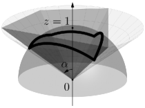
A proof of the previous lemma can be found in Appendix C.3. The statement is illustrated in Figure 3 for dimension . Observe that sliding along the edge linking with leaves the descent cone unchanged.

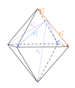
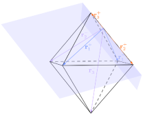
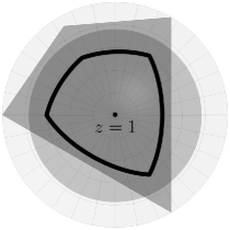
Whenever a convex cone contains a subspace, its circumangle is and the bound of Proposition 4.9 is not applicable. As can be seen in Figure 3, the descent cone of the -norm at contains the subspace spanned by the face of minimal dimension containing . To avoid this pitfall, let us recall the notion of lineality.
Definition 4.12 (Lineality [Roc70])
For a non-empty convex set , the lineality space of is defined as
| (4.19) |
It defines a subspace of and its dimension is referred to as the lineality of .
Any non-empty convex set can be expressed as the direct sum
| (4.20) |
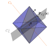
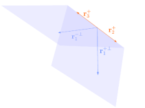
where is the orthogonal projection onto . The notation is used in analogy to the range in linear algebra. The set is “line-free” (i.e., its lineality is ) and its dimension is called the rank of . If is a convex cone, the lineality space is the largest subspace contained in and the circumangle of the range is less than . In the following, we will therefore apply Proposition 4.9 to the latter set only. Figure 4 illustrates the orthogonal decomposition of (4.20) for the descent cone of Figure 3.
The following lemma characterizes the lineality space and the range for descent cones of the -norm. A proof is given in Appendix C.3.
Lemma 4.13
Let be a vector with support and . The lineality space of is then given by
| (4.21) |
with lineality .
Notice that the lineality space is nothing but the face of the -ball of smallest dimension containing .
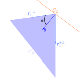
We now turn to the decomposition of the descent cone of the gauge into lineality space and range. To that end, let us first make the following simple observation.
Lemma 4.14 (Sign pattern of -representers)
All minimal -representers of with respect to share the same sign pattern, in the sense that for all , , the coordinate-wise product is nonnegative.
This lemma allows us to define the maximal -support.
Definition 4.15 (Maximal -support)
Let and be a dictionary. The maximal -support of in (or simply maximal support) is defined as . In what follows, we let denote its cardinality.
Since all solutions have the same sign pattern, any point in the relative interior of has maximal support. The next decomposition forms the main result of this section; see Appendix C.3 for a proof.
Proposition 4.16
Let be a dictionary and let . Let denote the descent cone of the gauge at . Let be any minimal -representer of in with maximal support and set as well as . Assume . Then we have:
-
(a)
The lineality space of has a dimension less than and is given by
(4.22) -
(b)
The range of is a -polyhedral -cone given by:
(4.23)
4.2.3 Consequence for the Sampling Rates
We now combine the main results of the previous two sections to derive an upper bound on the conic mean width of .
Theorem 4.17
A proof of the previous result is given in Appendix C.4. As a direct consequence, we get the following upper bound on the sampling rates for coefficient and signal recovery.
This result shows that robust coefficient and signal recovery is possible, when the number of measurements obeys . Hence, the sampling rate is mainly governed by the sparsity of maximal support -representations of in and the “narrowness” of the remaining cone , which is captured by its circumangle . The number of dictionary atoms only has a logarithmic influence. The next section is devoted to applying the previous result to various examples.
Remark 4.19
For the sake of clarity, the previous results are given in terms of the maximal sparsity. However, (potentially) more precise bounds can be achieved when replacing by . Furthermore note, that the proof of Theorem 4.17 reveals that is a necessary component in the required number of measurements. Indeed, since is a sharp description for the required number of measurements, equation (C.31) shows that the number of measurements for successful recovery is lower bounded by .
4.2.4 Examples
In this section, we discuss four applications of the previous upper bound on the conic mean width. First, we show that prediction for the required number of measurements agrees with the standard theory of compressed sensing. We then analytically compute the sampling rate of Corollary 4.18 for a specific scenario, in which the dictionary is formed by a concatenation of convolutions. The third example focuses on a numerical simulation in the case of 1D total variation. Lastly, we demonstrate how the circumangle can be controlled by the classical notion of coherence.
The Standard Basis
Our first example is dedicated to showing that the result of Corollary 4.18 is consistent with the standard theory of compressed sensing when . Hence, assume that we are given a sparse vector with and . Trivially, is then its own, unique -representation with respect to . According to Lemma 4.13, the -dimensional lineality space of is given by
| (4.25) |
where . For a simple calculation shows that where and . Furthermore, for it holds true that
| (4.26) |
so that the vectors generate a -polyhedral -cone with . Hence, Corollary 4.18 states that robust recovery of is possible for measurements. This bound is to be compared with the classical compressed sensing result, which prescribes to take measurements. Note that the slight difference in the logarithmic factor is due to our simple bound on , cf. Remark 4.10.
A Convolutional Dictionary
Consider a dictionary defined by the concatenation of two convolution matrices and with convolution kernels and , respectively. For instance, in dimension , this would yield the following matrix:
| (4.27) |
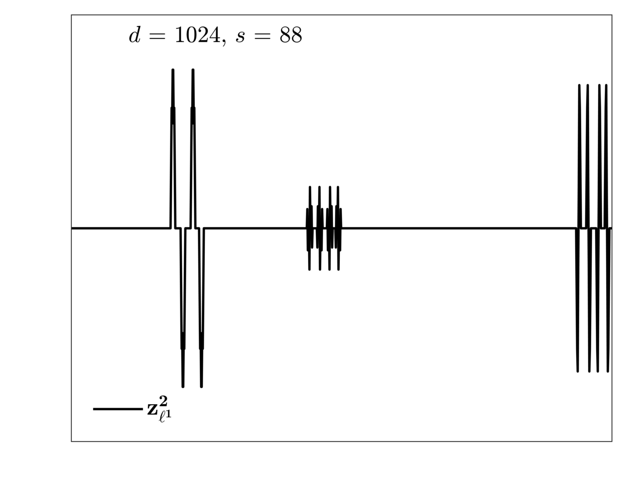
In particular for imaging applications, popular signal models are based on sparsity in such concatenations of convolutional matrices, e.g., translation invariant wavelets [Mal09] or learned filters in the convolutional sparse coding model [Woh14, BEL13]. Note that the resulting dictionary is highly redundant and correlated, so that existing coherence- and RIP-based arguments cannot provide satisfactory recovery guarantees. For the same reason, a recovery of a unique minimal -representer by () is unlikely, cf. the numerical simulation in Section 5.2. However, in the following, we will show how the previous upper bound based on the circumangle can be used in order to analyze signal recovery by ().
To that end, we consider the recovery of a simple vector supported on the first and the last component only, i.e., for all . A generalization to vectors supported on supports made of pairs of contiguous indices separated by pairs of contiguous zeros is doable, but we prefer this simple setting for didactic reasons. In this case, the set of minimal -representers can be completely characterized. Assuming additionally that , one can show that
Let denote any representer with maximal support and set . According to Proposition 4.16, we then decompose the descent cone into , where is the lineality space given by
and the range is given by . It is easy to see that , and that the projection on can be expressed as
The goal is now to show that is contained in a circular cone with angle and axis . Indeed, a straightforward computation shows that for we have
Hence, Corollary 4.18 implies that robust recovery of is possible for measurements.
1D Total Variation
As a third example we consider the problem of total variation minimization in 1D. Assume that and follow Model 1 with and that obeys Model 1.1. Total variation minimization is based on the assumption that is gradient-sparse, i.e., that , where denotes a discrete gradient operator, which is for instance based on forward differences with von Neumann boundary conditions. In order to recover from its noiseless, compressed measurements , one solves the program
| (4.28) |
For signals with it is easy to see that the previous formulation is equivalent to solving the synthesis basis pursuit () with , where denotes the Moore-Penrose inverse of .
The research of the past three decades demonstrates that encouraging a small total variation norm often efficaciously reflects the inherent structure of real-world signals. Although not as popular as its counterpart in 2D, total variation methods in one spatial dimension find application in many practical applications, see for instance [LJ11]. Somewhat surprisingly, Cai and Xu have shown that a uniform recovery of all -gradient-sparse signals is possible if and only if the number of (Gaussian) measurements obeys ; see [CX15]. Recently, [GMS20] has proven that this square-root bottleneck can be broken for signals with well separated jump discontinuities. This result is also based on establishing a non-trivial upper bound on the conic mean width. For such “natural” signals, measurements are already sufficient for exact recovery. See also [GLCS20, DHL17] for closely related results in a denoising context.
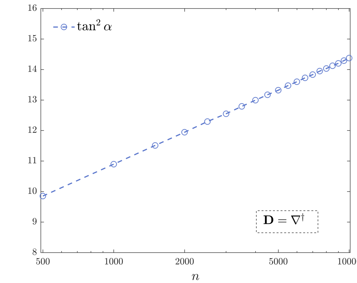
We want to demonstrate that the upper bound on the conic mean width based on the circumangle is capable of breaking the square-root bottleneck of the synthesis-based reformulation above. A theoretical analysis appears to be doable, however, it is beyond the scope of this work. Instead, we restrict ourselves to a simple numerical simulation. We consider signals that are defined by the pointwise discretization of a function on an interval with a few equidistant discontinuities and zero average. Note that for such a signal the unique minimal -representer with respect to is simply given by . Hence, we are only left with numerically computing the circumangle of the range in Proposition 4.16, which is done by means of Proposition 4.7. In order to confirm that required number of measurements scales logarithmically in the ambient dimension , we analyze the behavior of when the resolution is increased, i.e., for . The result is shown in Figure 5. The logarithmic scaling of (note that the -axis is logarithmic) indeed suggests that the bound of Corollary 4.18 predicts that measurements suffice for exact recovery. Hence, the presented upper bound based on the circumangle appears to be sharp enough to break the square-root bottleneck of total variation minimization in 1D.
Coherence and Circumangle
In our last example, we show that the circumangle of of Proposition 4.16 can be controlled in terms of the mutual coherence of the dictionary (see Equation (1.5)). This notion is a classical concept in the literature on sparse representations, which is frequently used to derive uniform recovery statements; see for instance [FR13, Chapter 5] for an overview. Note that the assumption of the following result guarantees that every -sparse is the unique minimal -representer of its associated signal [DE03, GN03]. Hence, in this situation, coefficient and signal recovery are equivalent, and both formulations are governed by the conic mean width of the cone .
Proposition 4.20
Let be a dictionary that spans with for and mutual coherence . Let denote an arbitrary -sparse vector with . Then the circumangle of the range of the descent cone obeys:
A proof of the previous result can be found in Appendix C.5. The statement allows us to retrieve a bound of the order for the needed number of measurements. For example, with , the bound of Corollary 4.18 results in a sampling rate of . Observe that this is essentially the same result as [RSV08, Corollary II.4], however, the constants of Proposition 4.20 are better controlled.
Note that the mutual coherence of a dictionary (sometimes also referred to as worst-case coherence [CK13, Chapter 9]) is a global quantity that is usually used to derive recovery guarantees that are uniform across all -sparse signals. Approaches based on this notion suffer from the so-called square-root bottleneck: The Welch bound [FR13, Theorem 5.7] reveals that the condition can only be satisfied for mild sparsity values . We emphasize that this is in contrast to the strategy of this work, which is tailored for a non-uniform recovery of individual signals. Indeed, the circumangle is a signal-dependent notion that allows to describe the local geometry.
5 Numerical Experiments
In this section, we illustrate our main findings regarding the -synthesis formulation by performing numerical simulations. First, we study the recovery of coefficient representations by (); see Section 5.1. In Section 5.2, we then focus on signal recovery by () in situations, where the identification of a coefficient representation is impossible. Section 5.3 is dedicated to the experiment of Figure 1, in which both formulations are compared. Lastly, we investigate the differences concerning robustness to measurement noise in Section 5.4. For general design principles and more details on our simulations we refer the interested reader to Appendix D.
To the best of our knowledge, all other compressed sensing results on the -synthesis formulation with redundant dictionaries describe the sampling rate as an asymptotic order bound. Hence, these results are not compatible with the experiments in this section and will not be further considered.
5.1 Sampling Rates for Coefficient Recovery
In order to study coefficient recovery by (), we create phase transition plots by running Experiment 5.1 for different dictionary and signal combinations reported below.
Experiment 5.1 (Phase transition for a fixed coefficient vector)
Input: Dictionary , coefficient vector .
Simulation Settings
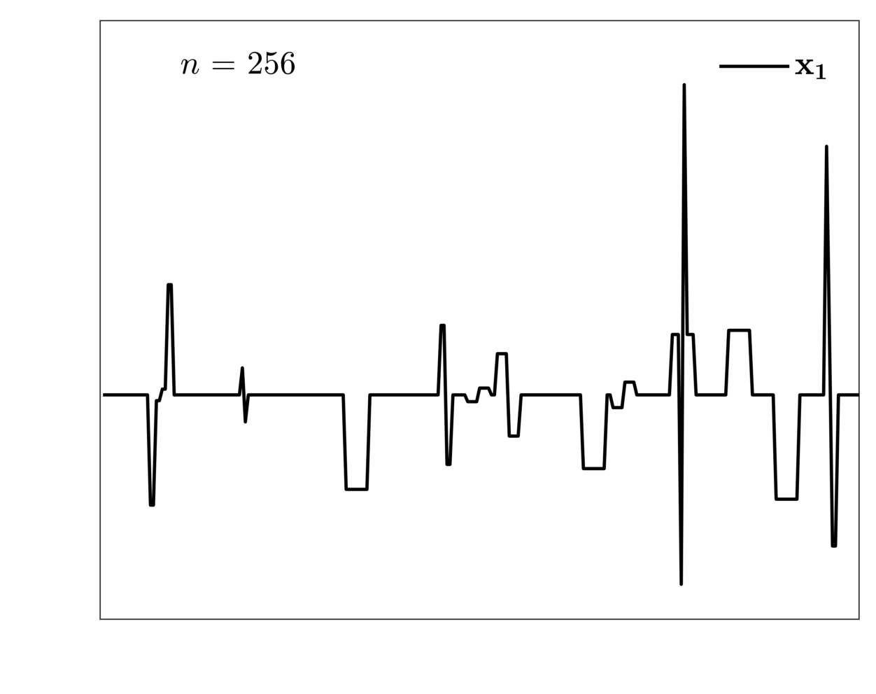
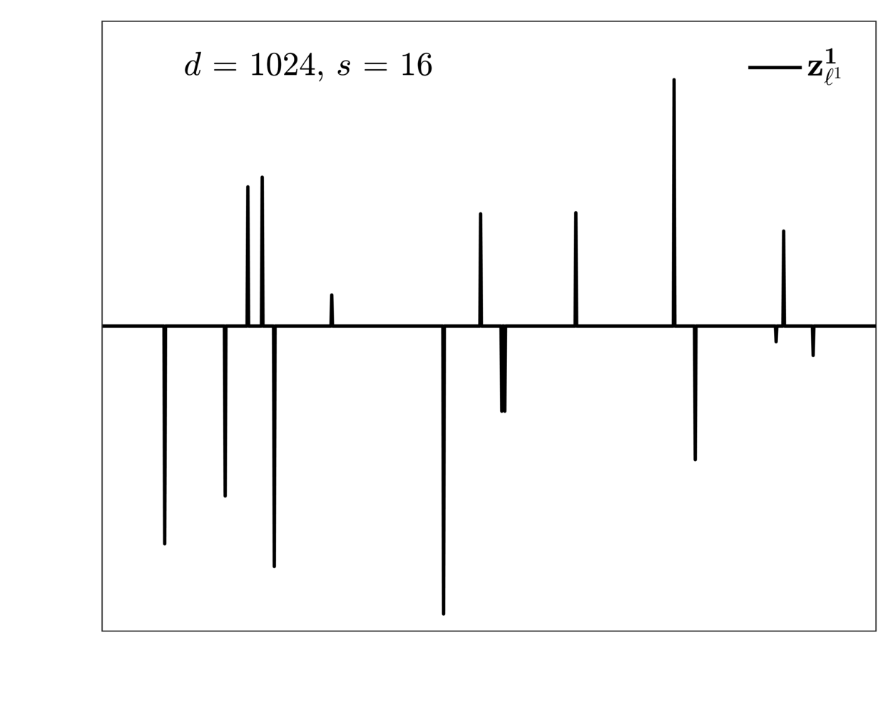
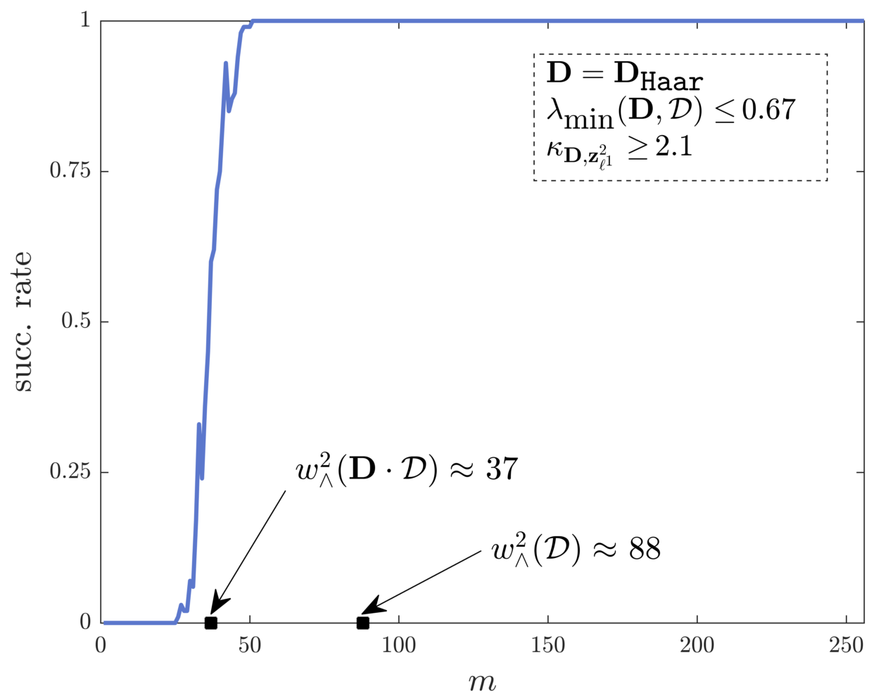
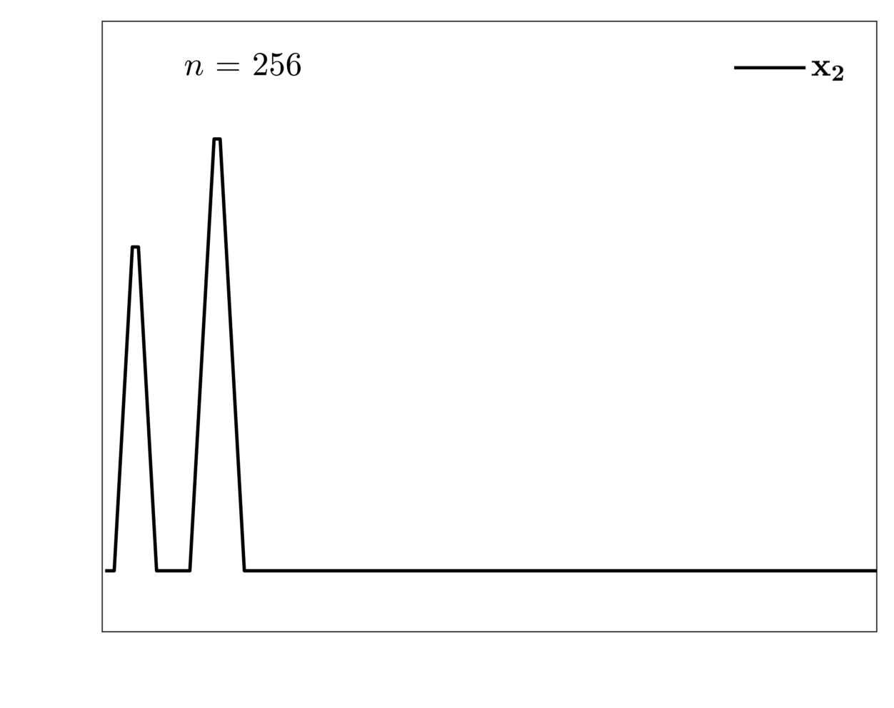
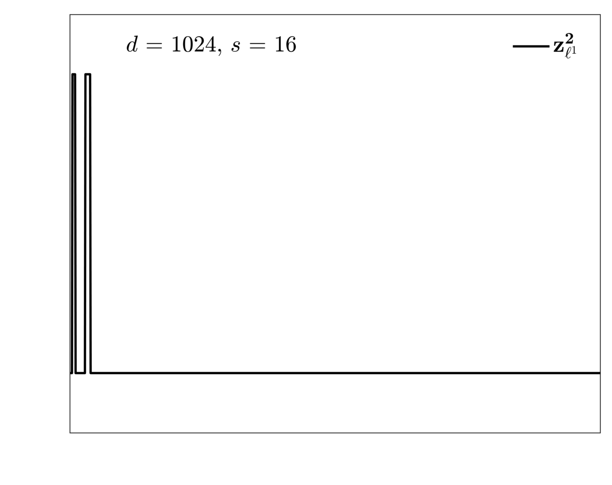
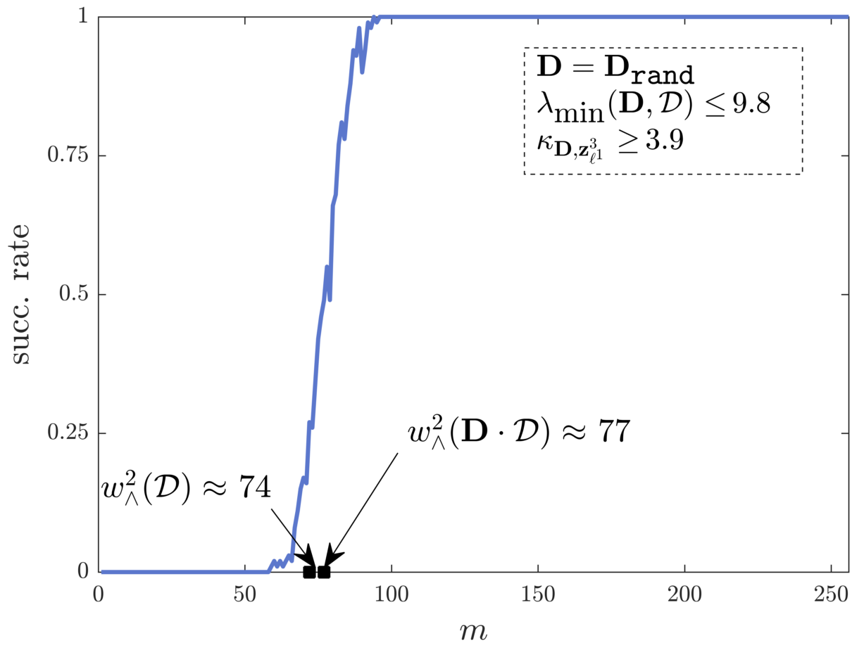
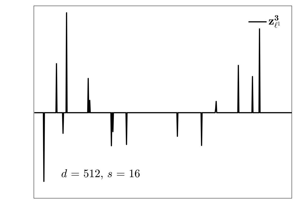
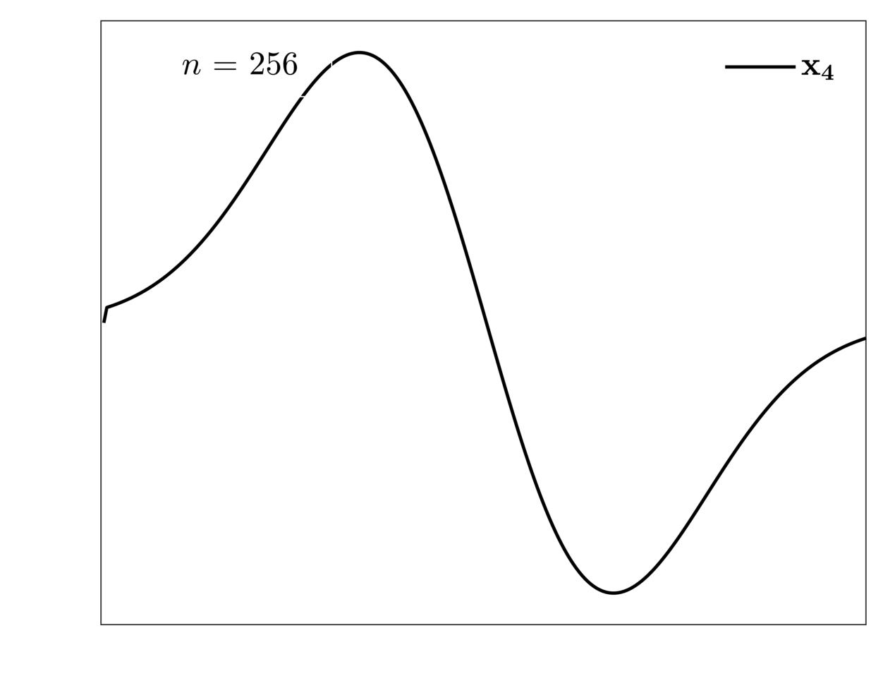
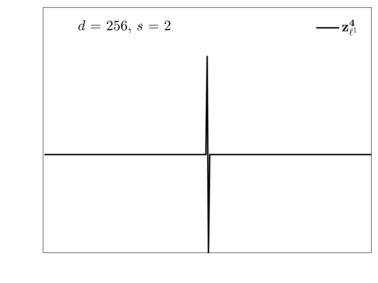
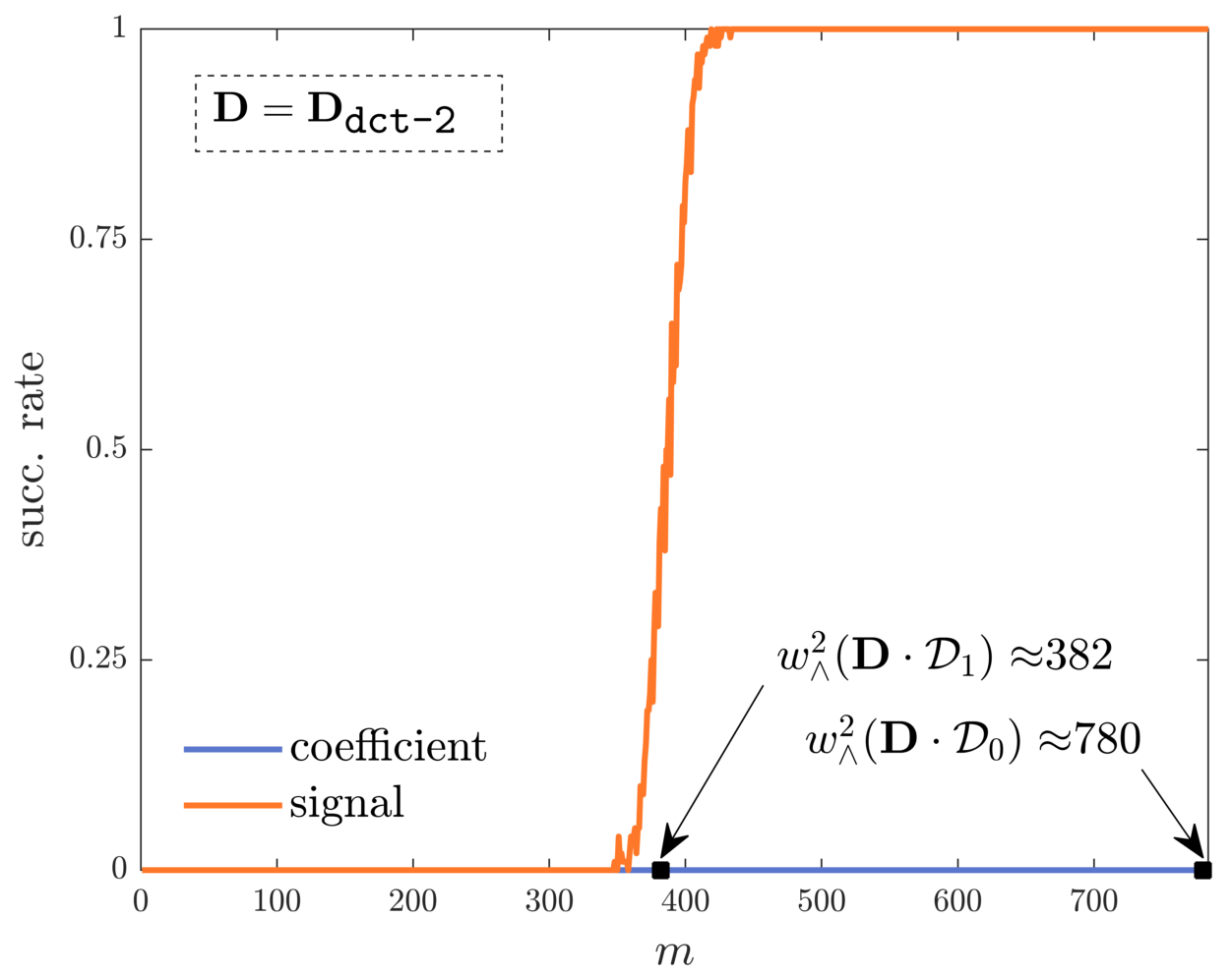
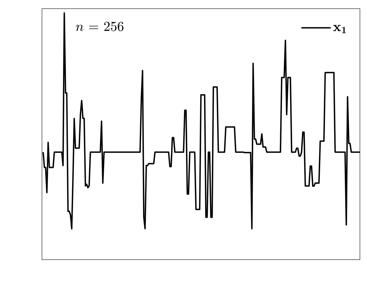
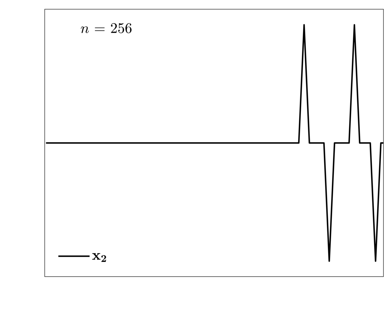
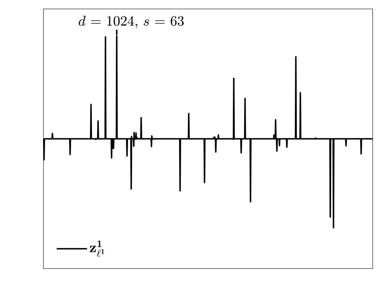
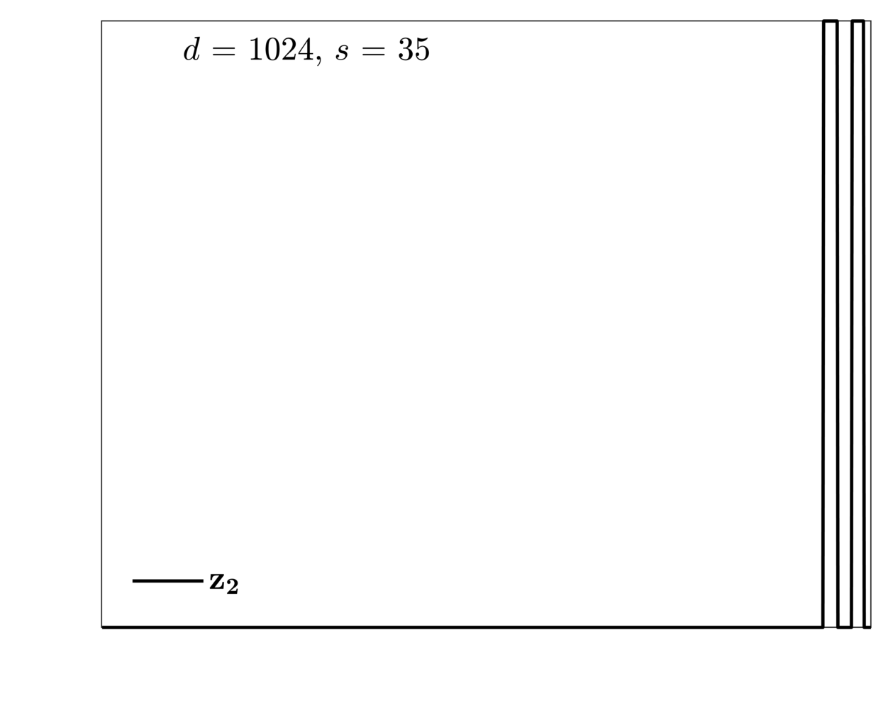
Our first two examples are based on a redundant Haar wavelet frame, which can be seen as a typical representation system in the field of applied harmonic analysis, see [Mal09] for more details on wavelets and Section 3.1 in [GKM20] for a short discussion in the context of compressed sensing. As a back-end for defining the wavelet transform, we are using the Matlab software package spot [BF13], which is in turn based on the Rice Wavelet Toolbox [B+17]. We set the ambient dimension to and consider a Haar system with decomposition levels and normalized atoms. The resulting dictionary is denoted by . The first coefficient vector is obtained by selecting a random support set of cardinality , together with random coefficients; see Subfigure 6(c) for a visualization of and Subfigure 6(b) for the resulting signal . The second coefficient vector is created by defining two contiguous blocks of non-zero coefficients in the low frequency part, again with ; see Subfigure 6(f) for a plot of and Subfigure 6(e) for the resulting signal . For each signal we run Experiment 5.1 and report the empirical success rate in the Subfigures 6(a), 6(d), respectively.
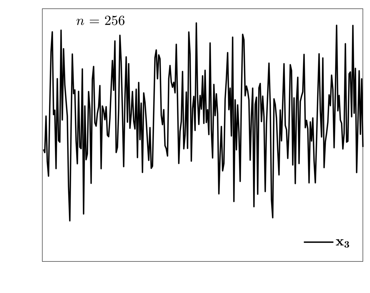
In the third example, the dictionary is chosen as a Gaussian random matrix, which is a typical benchmark system for compressed sensing with redundant frames, see for instance [GKM20, KR15, CWW14]. Also in this case, we set , but we choose . The resulting dictionary is denoted by . The coefficient vector is defined in the same manner as above (see Subfigure 6(i)), where we again have . The resulting signal is shown in Subfigure 6(h) and the empirical success rate in Subfigure 6(g).
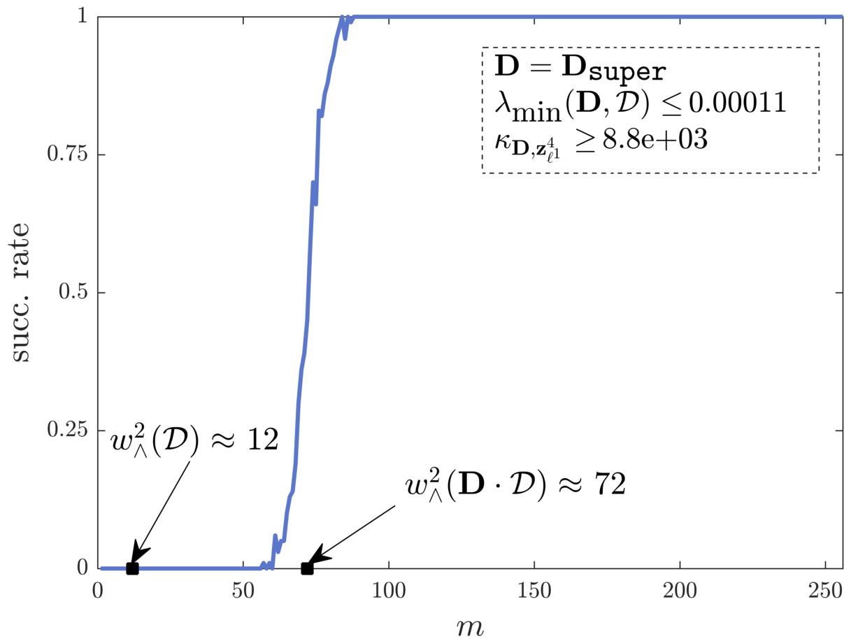
Our fourth and last dictionary is inspired by super-resolution; see for instance [CF14]. We again set and choose the dictionary as a convolution with a discrete Gaussian function of large variance. This example can therefore be considered as a finely discretized super-resolution problem. The coefficient vector is then chosen as a sparse vector with and , see Subfigure 6(l). Hence, in the signal , the two neighboring peaks almost cancel out and result in the low amplitude signal shown in Subfigure 6(k). Finally, the empirical success rate is depicted in Subfigure 6(j). Note that for each example we have verified the condition heuristically by verifying that , respectively.
Results
Let us now analyze the empirical success rates of Figure 6 and compare them with the estimates of and . Our findings are summarized in the following:
-
(i)
The convex program () obeys a sharp phase transition in the number of measurements : Recovery of a coefficient vector fails if is below a certain threshold and succeeds with overwhelming probability once a small transition region is surpassed. This observation could have been anticipated, given for instance the works [ALMT14, Tro15]. However, note that the product structure of the matrix in () does not allow for a direct application of these results.
- (ii)
- (iii)
-
(iv)
For two minimal -representations with the same sparsity, but with different supports, the quantities and might differ significantly, while ; see Subfigures 6(a) and 6(d). Hence, sparsity alone does not appear to be a good proxy for the sampling complexity of (). A refined understanding of coefficient recovery requires a theory that is non-uniform across the class of all -sparse signals.
-
(v)
The local condition number might explode, which often renders a condition bound as in Proposition 4.3 unusable. Indeed, we report upper bounds for in the first column of Figure 6. Since the norms of each dictionary are well controlled, this quantity is responsible for the large values of the local condition number.
5.2 Sampling Rates for Signal Recovery
For the investigation of signal recovery via (), we also create phase transition plots by running Experiment 5.1 for different dictionary and signal combinations. Note that we also compute and store the signal error in the third step of the experiment (in addition to ). Recovery is declared successful if .
Simulation Settings
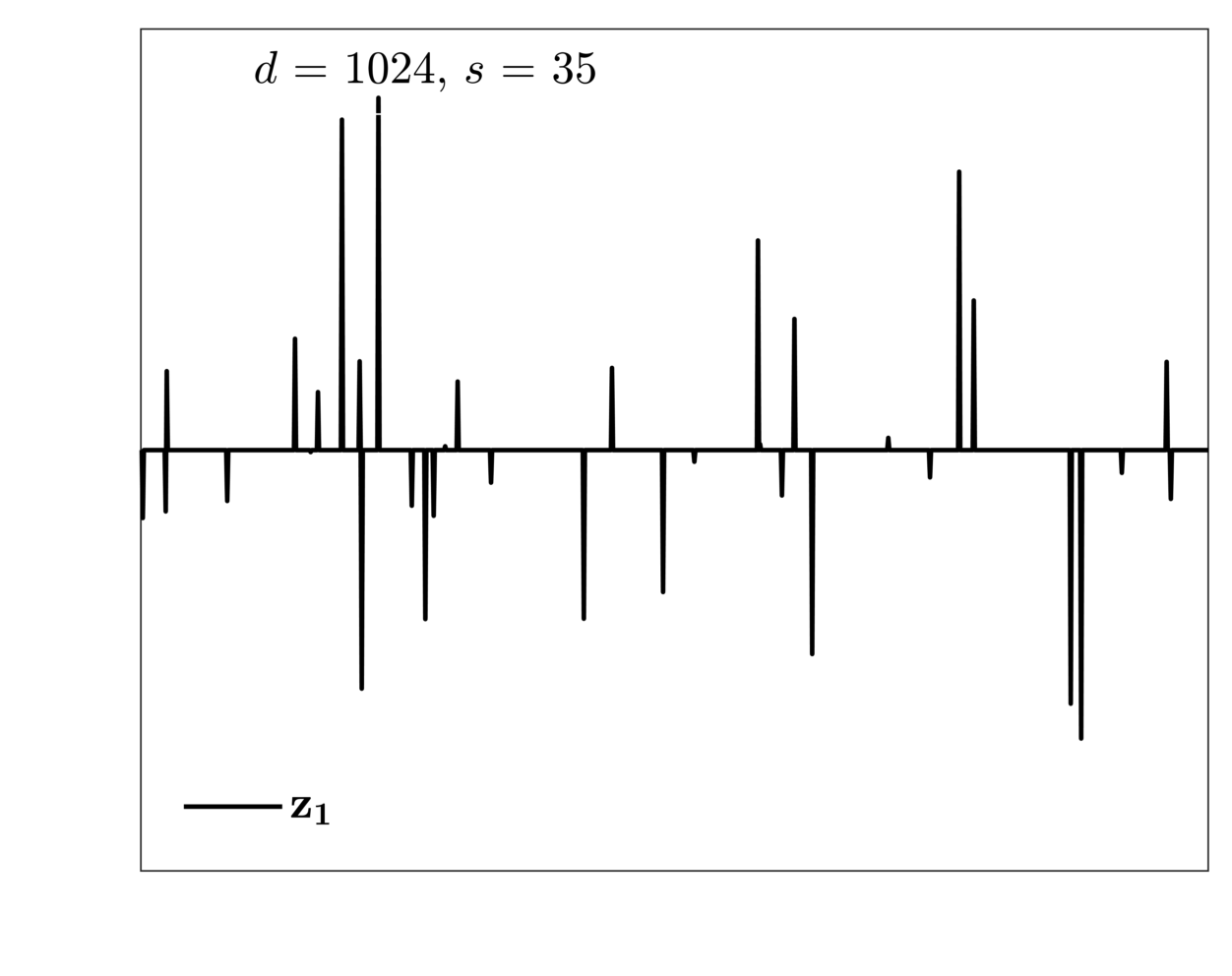
Our first two examples are based on the same Haar wavelet system with 3 decomposition levels that is used in Section 5.1. The first signal is constructed by defining a coefficient vector with a random support set of cardinality and random coefficients; see Subfigure 7(j) for a visualization of and Subfigure 7(d) for the resulting signal . In order to apply the result of Theorem 3.8, we compute a minimal -representer of ; see Subfigure 7(g). The second coefficient vector is created by defining two contiguous blocks of non-zero coefficients in a lower frequency decomposition scale, again with ; see Subfigure 7(k) for a plot of and Subfigure 7(e) for the resulting signal . A corresponding minimal -representer of is shown in Subfigure 7(h).
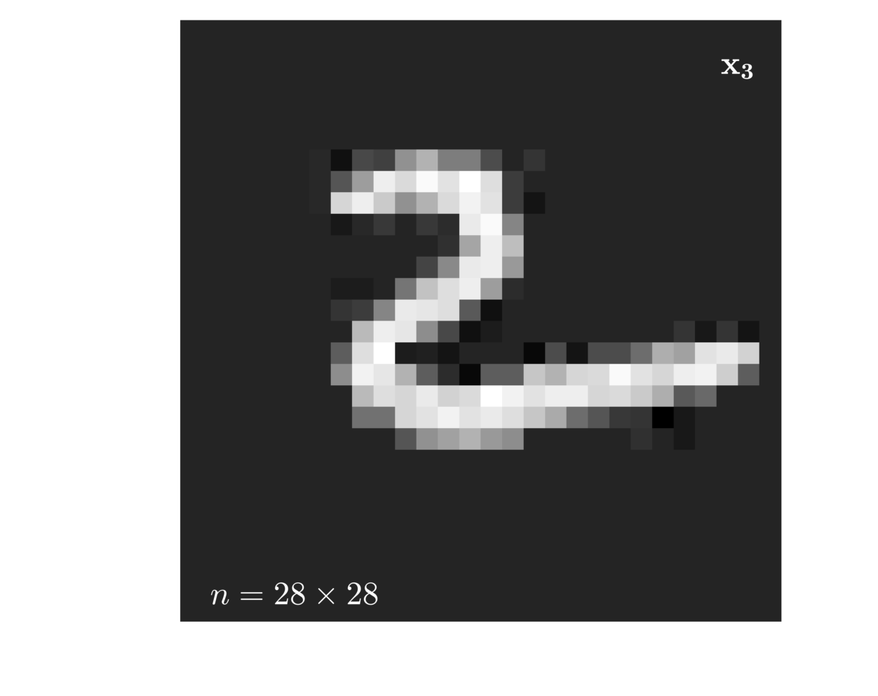
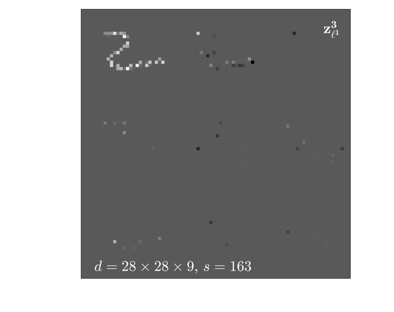
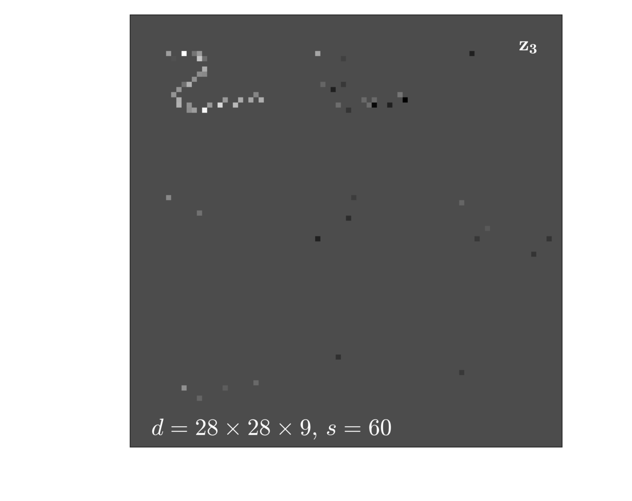
Finally, for the third setup we are choosing a simple example in 2D. In order to keep the computational burden manageable, we restrict ourselves to a -dimensional digit from the MNIST data set [LBBH98], i.e., the vectorized image is of size . As a sparsifying system we utilize a dictionary that is based on the 2D discrete cosine transform (dct-2). It makes use of Matlab’s standard dct-2 transform as convolution filters on patches. The resulting operator is denoted by , i.e., . Note that such a convolution sparsity model is frequently used in the literature, in particular also with learned filters, e.g., see convolutional sparse coding in [BEL13]. Although the dct-2 filters might not be a perfect match for MNIST digits, we consider them as a classical representative that is well suited to demonstrate the predictive power of our results. In order to construct a suitable sparse representation of an arbitrarily picked digit in the database, we make use of the orthogonal matching pursuit algorithm [PRK93]; see Subfigure 7(l) for a visualization of . The resulting digit is displayed in Figure 7(f). A minimal -representer , which is needed to apply Theorem 3.8, is shown in Subfigure 7(i).
Results
Our conclusions on the numerical experiments shown in Figure 7 are reported in the following:
-
(vi)
The convex program () obeys a sharp phase transition in the number of measurements. Due to the equivalent, gauge-based reformulation (3.1) of (), this observation is predicted by the works [ALMT14, Tro15]. However, a recovery of a coefficient representation via solving () is impossible in all three examples, even for .
- (vii)
-
(viii)
In contrast, for any other sparse representation , the conic width does not describe the sampling rate of (), in general. Indeed, observe that we have in all three examples. Also note that , however, the locations of the phase transitions deviate considerably. Similarly, although , we have that . This observation is yet another indication that sparsity alone is not a good proxy for the sampling rate of -synthesis, in general.
5.3 Creating a “Full” Phase Transition
Let us now focus on the phase transition plots shown in Figure 1. Up to now, we have only considered one specific signal at a time. However, it is also of interest to assess the quality of our results if the “complexity” of the underlying signals is varied. In the classical situation of being an ONB, the location of the phase transition is entirely determined by the sparsity of the underlying signal. Hence, it is a natural choice to create phase transitions over the sparsity, as it is for instance done in [ALMT14]. Recalling Claims (iv) and (viii), it might appear odd to do the same in the case of a redundant dictionary. However, as the result of Figure 1 shows, if the support is chosen uniformly at random, sparsity is still a somewhat reasonable proxy for the sampling rate. Indeed, these plots are created by running Experiment 5.2 with , maximal sparsity and displaying the empirical success rates of coefficient and signal recovery, respectively. Additionally the dotted line shows the averaged conic mean width values .
Experiment 5.2 (Phase transition of Figure 1)
Input: Dictionary , maximal sparsity .
Compute: Repeat the following procedure times for each :
-
Select a set uniformly at random with . Then draw a standard Gaussian random vector and define by setting and .
-
Define the signal and compute a minimal -representation of . Compute the conic mean width .
-
Run Experiment 5.1 with and as input, where the number of repetitions is lowered to 5. In the third step, coefficient/signal recovery is declared successful if or if , respectively.
First note, that the averaged values of the conic mean width perfectly match the center of the phase transition of() in Subfigure 1(b), as it is predicted by Theorem 3.8. However, observe that for sparsity values between and the transition region is spread out in the vertical direction, cf. [ALMT14]. This phenomenon can be related to Claim (viii): Given that sparsity alone is not a good proxy for the sample complexity of (), averaging over different instances with the same sparsity necessarily results in a smeared out transition area.
Regarding the phase transition in Subfigure 1(a), we observe that the location of the phase transition is also determined by ; provided that coefficient recovery is possible, i.e., if . For sparsity values , recovery of coefficients appears to be impossible, whereas signal and coefficient recovery seems to be equivalent for very small sparsity values (i.e., ). The interval in between forms a transition region, in which coefficient recovery becomes gradually less likely. We suspect that with more repetitions in Experiment 5.2, the empirical success rates on this interval would eventually smooth out.
We conclude that:
-
(ix)
Whether , i.e., whether coefficient recovery is possible, is again a property that is non-uniform in the sparsity of .
5.4 Robustness to Noise
The purpose of this last numerical simulation is to analyze coefficient and signal recovery with respect to robustness to measurement noise. To that end, we run Experiment 5.3 for different setups, which are reported below.
Experiment 5.3 (Robustness to Measurement Noise)
Input: Dictionary , number of measurements , minimal -representation of the signal , range of noise levels .
Simulation settings
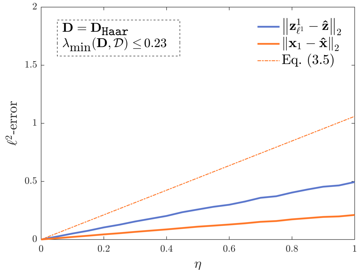
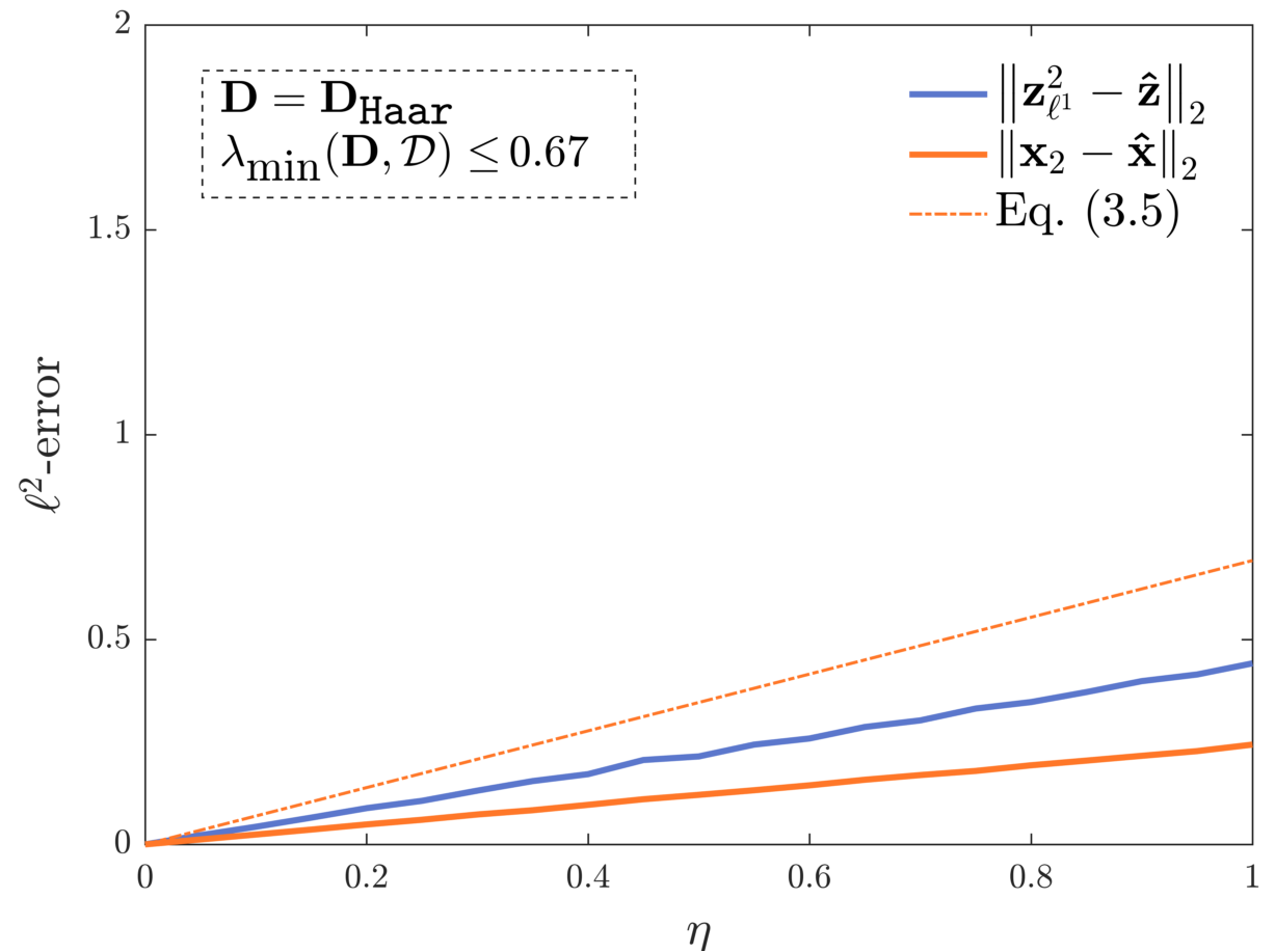
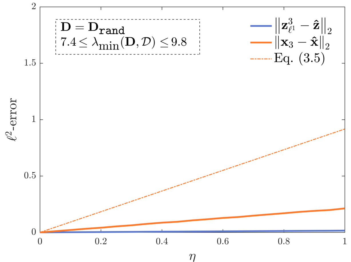
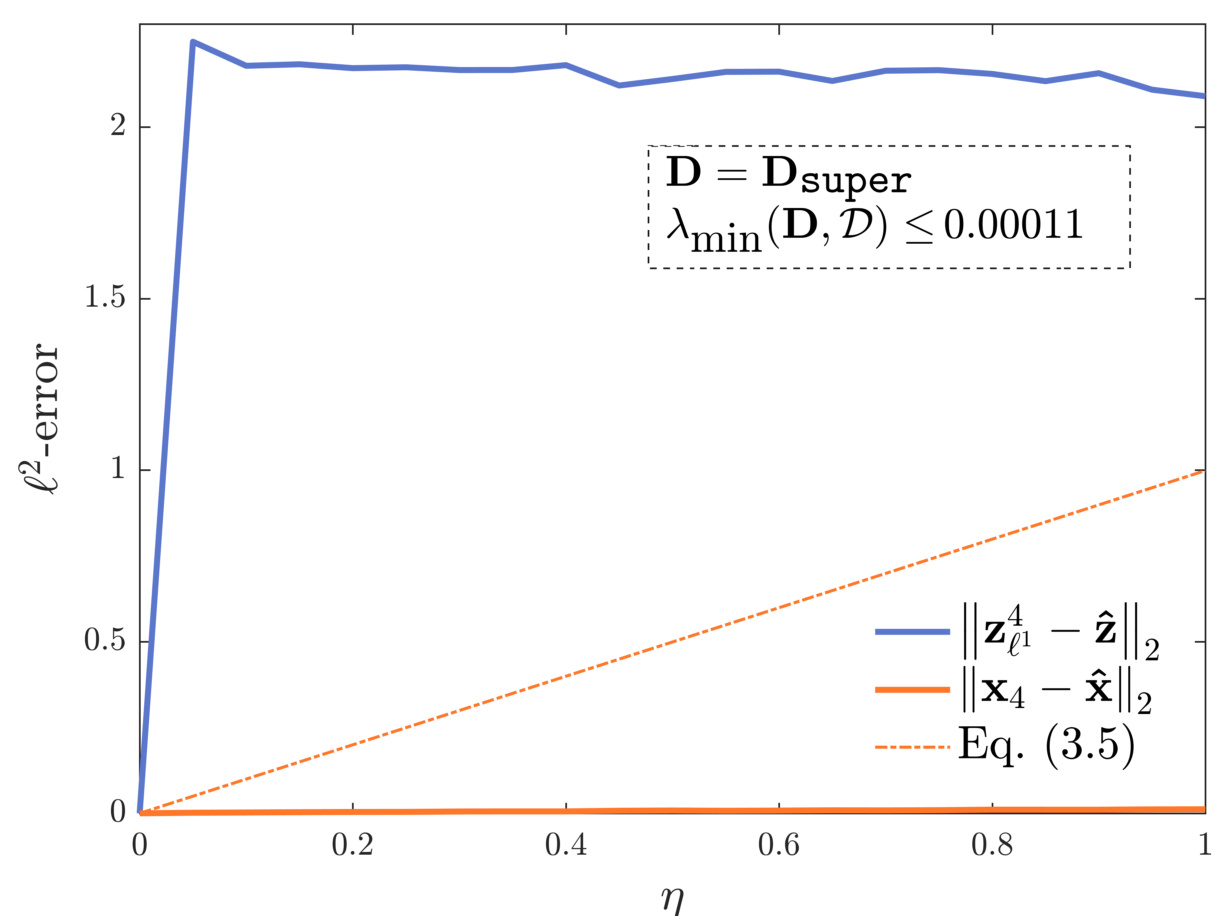
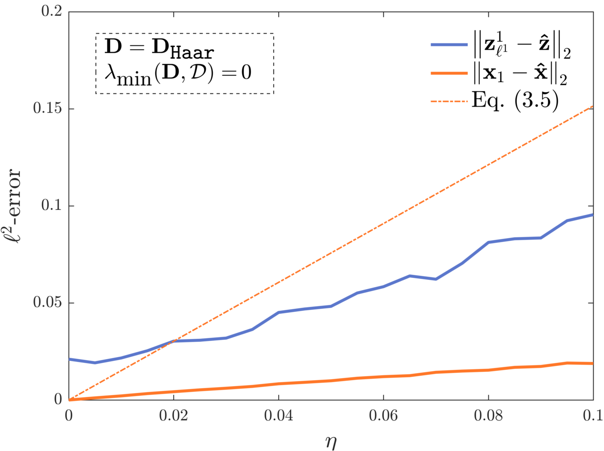
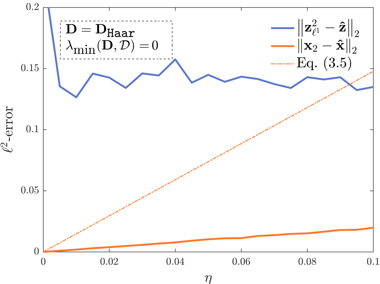
First, we choose the same dictionary and signal combination as in Section 5.1 and restrict the noise level to . Furthermore, we consider the 1D examples of Section 5.2, together with the noise range . Recall that the difference of these two setups is that in the first case, whereas in the second case. In all experiments, we roughly pick the number of measurements as to ensure that Theorem 3.6 (or Theorem 3.8, respectively) is applicable. The averaged coefficient and signal recovery errors are displayed in Figure 8, together with the theoretical upper bound on the signal error of Equation (3.6). Note that it is not possible to show the corresponding error bound for coefficient recovery. In the first set of examples, we do not have access to and in the last two cases, and therefore Theorem 3.6 is not applicable. Nevertheless, it is possible to obtain an upper bound for the latter quantity, as outlined in the Appendix D. If , it is additionally possible to use the result on minimum conic singular values of Gaussian matrices to get a lower bound with high probability [Tro15, Proposition 3.3].
Results
We summarize the findings of the results shown in Figure 8 below:
-
(x)
If the number of measurements exceeds the sampling rate in Theorem 3.8, signal recovery via solving the Program () is robust to measurement noise. This phenomenon holds true without any further assumptions. Indeed, observe that in all simulations of Figure 8, the signal error lies below its theoretical upper bound of Equation (3.6).
-
(xi)
If is the unique minimal -representation of (i.e., if ) and if the number of measurements exceeds the sampling rate in Theorem 3.6, it is possible to robustly recovery . However, in contrast to signal recovery, the robustness is influenced by the “stability” of the minimal -representation of in , i.e., by the value of in the error bound (3.4). Indeed, it is possible that the signal is more robustly recovered than its coefficients , or vice versa. This can be seen by comparing coefficient and signal recovery in the Subfigures 8(a)-8(d).333Note that the quantity is very small. Hence, even for a small amount of noise the error of Equation (3.4) explodes. For the error stays roughly constant since the solution of () is always close to . If , coefficient recovery is less robust than signal recovery, see Subfigures 8(a), 8(b) and 8(d). However, if , the contrary holds true, see Subfigure 8(c).
Acknowledgments
Acknowledgements: M.M. is supported by the DFG Priority Programme DFG-SPP 1798. He wishes to thank Martin Genzel for inspiring discussions. C.B. have been supported by a PEPS « Jeunes chercheuses et jeunes chercheurs » funding in 2017 and 2018 for this work. P.W. and J.K. are supported by the ANR JCJC OMS.
References
- [ALMT14] Dennis Amelunxen, Martin Lotz, Michael B. McCoy and Joel A. Tropp “Living on the edge: phase transitions in convex programs with random data” In Inf. Inference 3.3, 2014, pp. 224–294
- [ALW20] D. Amelunxen, M. Lotz and J. Walvin “Effective condition number bounds for convex regularization” in press In IEEE Trans. Inf. Theory, 2020
- [B+17] Richard Baraniuk, Hyeokho Choi and Ramesh Neelamani “Rice Wavelet Toolbox, Version 3”, URL: https://github.com/ricedsp/rwt, 2017
- [BEL13] H. Bristow, A. Eriksson and S. Lucey “Fast Convolutional Sparse Coding” In 2013 IEEE Conference on Computer Vision and Pattern Recognition, 2013
- [Beu38] A. Beurling “Sur les intégrales de Fourier absolument convergentes et leur application à une transformation fonctionnelle” In Ninth Scandinavian Mathematical Congress, 1938, pp. 345–366
- [BF13] Ewout Berg and Michael P. Friedlander “Spot – A Linear-Operator Toolbox”, URL: http://www.cs.ubc.ca/labs/scl/spot/index.html, 2013
- [BM02] Peter L. Bartlett and Shahar Mendelson “Rademacher and Gaussian complexities: Risk bounds and structural results” In J. Mach. Learn. Res. 3, 2002, pp. 463–482
- [CCL19] Peter G. Casazza, Xuemei Chen and Richard G. Lynch “Preserving Injectivity under Subgaussian Mappings and Its Application to Compressed Sensing” arXiv preprint: 1710.09972, 2019
- [CDS98] S. Chen, D. Donoho and M. Saunders “Atomic Decomposition by Basis Pursuit” In SIAM J. Sci. Comput. 20.1, 1998, pp. 33–61
- [CENR11] Emmanuel J. Candès, Yonina C. Eldar, Deanna Needell and Paige Randall “Compressed sensing with coherent and redundant dictionaries” In Appl. Comput. Harmon. Anal. 31.1, 2011, pp. 59–73
- [CF14] Emmanuel J. Candès and Carlos Fernandez-Granda “Towards a Mathematical Theory of Super-resolution” In Commun. Pur. Appl. Math. 67.6, 2014, pp. 906–956
- [CK13] “Finite Frames: Theory and Applications”, Applied and Numerical Harmonic Analysis Birkhäuser, 2013
- [CM73] J.. Claerbout and F. Muir “Robust Modeling With Erratic Data” In Geophysics 38.5, 1973, pp. 826–844
- [CR06] Emmanuel J Candès and Justin Romberg “Quantitative robust uncertainty principles and optimally sparse decompositions” In Found. Comput. Math. 6.2 Springer, 2006, pp. 227–254
- [CRPW12] Venkat Chandrasekaran, Benjamin Recht, Pablo A. Parrilo and Alan S. Willsky “The convex geometry of linear inverse problems” In Found. Comput. Math. 12.6, 2012, pp. 805–849
- [CRT06] E.. Candès, J. Romberg and T. Tao “Robust Uncertainty Principles: Exact Signal Reconstruction from Highly Incomplete Frequency Information” In IEEE Trans. Inf. Theor. 52.2, 2006, pp. 489–509
- [CRT06a] Emmanuel J. Candès, Justin K. Romberg and Terence Tao “Stable signal recovery from incomplete and inaccurate measurements” In Comm. Pure Appl. Math. 59.8, 2006, pp. 1207–1223
- [CT06] E.. Candès and T. Tao “Near-Optimal Signal Recovery From Random Projections: Universal Encoding Strategies?” In IEEE Trans. Inf. Theor. 52.12, 2006, pp. 5406–5425
- [CWW14] Xuemei Chen, Haichao Wang and Rongrong Wang “A null space analysis of the -synthesis method in dictionary-based compressed sensing” In Appl. Comput. Harmon. Anal. 37.3, 2014, pp. 492–515
- [CX15] Jian-Feng Cai and Weiyu Xu “Guarantees of total variation minimization for signal recovery” In Inf. Inference 4.4, 2015, pp. 328–353
- [DE03] D.. Donoho and M. Elad “Optimally sparse representation in general (nonorthogonal) dictionaries via minimization” In Proc. Natl. Acad. Sci. 100.5, 2003, pp. 2197–2202
- [DH01] D.. Donoho and X. Huo “Uncertainty principles and ideal atomic decomposition” In IEEE Trans. Inf. Theory 47.7, 2001, pp. 2845–2862
- [DHL17] Arnak S. Dalalyan, Mohamed Hebiri and Johannes Lederer “On the prediction performance of the Lasso” In Bernoulli 23.1, 2017, pp. 552–581
- [DNW13] M.. Davenport, D. Needell and M.. Wakin “Signal Space CoSaMP for Sparse Recovery With Redundant Dictionaries” In IEEE Trans. Inf. Theory 59.10, 2013, pp. 6820–6829
- [Don06] David L. Donoho “Compressed sensing” In IEEE Trans. Inf. Theory 52.4, 2006, pp. 1289–1306
- [EB02] Michael Elad and Alfred M Bruckstein “A Generalized Uncertainty Principle and Sparse Representation in Pairs of Bases” In IEEE Trans. Inf. Theory 48.9 Citeseer, 2002
- [EMR07] M. Elad, P. Milanfar and R. Rubinstein “Analysis versus synthesis in signal priors” In Inverse Probl. 23.3, 2007, pp. 947–968
- [FR13] Simon Foucart and Holger Rauhut “A Mathematical Introduction to Compressive Sensing”, Applied and Numerical Harmonic Analysis Birkhäuser, 2013
- [Fuc04] J.-J. Fuchs “On sparse representations in arbitrary redundant bases” In IEEE Trans. Inf. Theory 50.6, 2004, pp. 1341–1344
- [Fuc05] Jean-Jacques Fuchs “Recovery of exact sparse representations in the presence of bounded noise” In IEEE Trans. Inf. Theory 51.10 IEEE, 2005, pp. 3601–3608
- [FV99] Robert M. Freund and Jorge R. Vera “Condition-Based Complexity of Convex Optimization in Conic Linear Form via the Ellipsoid Algorithm” In SIAM J. Optim. 10.1, 1999, pp. 155–176
- [GB08] Michael Grant and Stephen Boyd “Graph implementations for nonsmooth convex programs” In Recent Advances in Learning and Control 371, Lecture Notes in Control and Information Sciences Springer London, 2008, pp. 95–110
- [GB14] Michael Grant and Stephen Boyd “CVX: Matlab Software for Disciplined Convex Programming, version 2.1”, URL: http://cvxr.com/cvx, 2014
- [GKM20] M. Genzel, G. Kutyniok and M. März “-Analysis Minimization and Generalized (Co-)Sparsity: When Does Recovery Succeed?” Accepted, arXiv preprint: 1710.04952 In Appl. Comput. Harmon. Anal., 2020
- [GLCS20] Adityanand Guntuboyina, Donovan Lieu, Sabyasachi Chatterjee and Bodhisattva Sen “Adaptive risk bounds in univariate total variation denoising and trend filtering” In Ann. Statist. 48.1, 2020, pp. 205–229
- [GM04] A.. Giannopoulos and V.. Milman “Asymptotic Convex Geometry Short Overview” In Different Faces of Geometry Springer, 2004, pp. 87–162
- [GMS20] M. Genzel, M. März and R. Seidel “Compressed Sensing with 1D Total Variation: Breaking Sample Complexity Barriers via Non-Uniform Recovery” arXiv preprint: 2001.09952, (2020) arXiv:2001.09952
- [GN03] R. Gribonval and M. Nielsen “Sparse representations in unions of bases” In IEEE Trans. Inf. Theory 49.12, 2003, pp. 3320–3325
- [GNEGD14] R. Giryes, S. Nam, M. Elad, R. Gribonval and M.. Davies “Greedy-like algorithms for the cosparse analysis model” In Linear Algebra Appl. 441, 2014, pp. 22–60
- [Gor85] Yehoram Gordon “Some inequalities for Gaussian processes and applications” In Isr. J. Math. 50.4, 1985, pp. 265–289
- [Gor88] Yehoram Gordon “On Milman’s inequality and random subspaces which escape through a mesh in ” In Geometric aspects of functional analysis 1317, Lecture Notes in Mathematics Springer, 1988, pp. 84–106
- [HS10] R Henrion and A. Seeger “On Properties of Different Notions of Centers for Convex Cones” In Set-Valued Anal. 18, 2010, pp. 205–231
- [HS10a] René Henrion and Alberto Seeger “Inradius and Circumradius of Various Convex Cones Arising in Applications” In Set-Valued Anal. 18, 2010, pp. 483–511
- [HS10b] J-B Hiriart-Urruty and Alberto Seeger “A variational approach to copositive matrices” In SIAM Rev. 52.4, 2010, pp. 593–629
- [IS08] A. Iusem and A. Seeger “Normality and modulability indices. Part I: Convex cones in normed spaces” In J. Math. Anal. Appl. 338.1, 2008, pp. 365–391
- [KNW15] Felix Krahmer, Deanna Needell and Rachel Ward “Compressive Sensing with Redundant Dictionaries and Structured Measurements” In SIAM J. Math. Anal. 47.6, 2015, pp. 4606–4629
- [KR15] Maryia Kabanava and Holger Rauhut “Analysis -recovery with Frames and Gaussian Measurements” In Acta Appl. Math. 140.1, 2015, pp. 173–195
- [Kre38] M.G. Kreǐn “The L-problem in an abstract normed linear space” English Transl. Amer. Math. Soc., Providence, R.I., 1962. MR 29 # 5073 In Some questions in the theory of moments Gos. Naučno-Tehn. Izdat. Ukraine, 1938
- [KRZ15] M. Kabanva, H. Rauhut and H. Zhang “Robust analysis -recovery from Gaussian measurements and total variation minimization” In Eur. J. Appl. Math. 26.6, 2015, pp. 917–929
- [LBBH98] Yann LeCun, Léon Bottou, Yoshua Bengio and Patrick Haffner “Gradient-based learning applied to document recognition” In Proc. IEEE 86.11, 1998, pp. 2278–2324
- [LJ11] Max A. Little and Nick S. Jones “Generalized methods and solvers for noise removal from piecewise constant signals. I. Background theory” In Proc. Royal Soc. Lond. A 467.2135, 2011, pp. 3088–3114
- [LLMLY12] Y. Liu, S. Li, T. Mi, H. Lei and W. Yu “Performance analysis of -synthesis with coherent frames” In 2012 IEEE International Symposium on Information Theory Proceedings, 2012, pp. 2042–2046
- [LMPV17] Christopher Liaw, Abbas Mehrabian, Yaniv Plan and Roman Vershynin “A Simple Tool for Bounding the Deviation of Random Matrices on Geometric Sets” In Geometric Aspects of Functional Analysis 2169, Lecture Notes in Mathematics Springer, 2017, pp. 277–299
- [Log65] B. Logan “Properties of High-Pass Signals”, 1965
- [Mal09] S. Mallat “Cover image A Wavelet Tour of Signal Processing: The Sparse Way” Elsevier, 2009
- [Mil85] V.. Milman “Random subspaces of proportional dimension of finite dimensional normed spaces: Approach through the isoperimetric inequality” In Banach Spaces 1166, Lecture Notes in Mathematics Springer Berlin Heidelberg, 1985, pp. 106–115
- [MK87] Katta G Murty and Santosh N Kabadi “Some NP-complete problems in quadratic and nonlinear programming” In Math. Program. 39.2 Springer, 1987, pp. 117–129
- [MPT07] Shahar Mendelson, Alain Pajor and Nicole Tomczak-Jaegermann “Reconstruction and subgaussian operators in asymptotic geometric analysis” In Geom. Funct. Anal. 17.4, 2007, pp. 1248–1282
- [MZ93] S.. Mallat and Zhifeng Zhang “Matching pursuits with time-frequency dictionaries” In IEEE Trans. Signal Process. 41.12, 1993, pp. 3397–3415
- [NDEG13] S. Nam, M.. Davies, M. Elad and R. Gribonval “The cosparse analysis model and algorithms” In Appl. Comput. Harmon. Anal. 34.1, 2013, pp. 30–56
- [PRK93] Y.. Pati, R. Rezaiifar and P.. Krishnaprasad “Orthogonal matching pursuit: recursive function approximation with applications to wavelet decomposition” In Proceedings of 27th Asilomar Conference on Signals, Systems and Computers, 1993, pp. 40–44 vol.1
- [Ren95] J. Renegar “Linear programming, complexity theory and elementary functional analysis” In Math. Program. 70, 1995, pp. 279–351
- [Roc70] Ralph Tyrell Rockafellar “Convex Analysis” Princeton University Press, 1970
- [ROF92] L. Rudin, S. Osher and E. Fatemi “Nonlinear total variation based noise removal algorithms” In Physica D 60.1–4, 1992, pp. 259–268
- [RSV08] H. Rauhut, K. Schnass and P. Vandergheynst “Compressed Sensing and Redundant Dictionaries” In IEEE Trans. Inf. Theory 54.5, 2008, pp. 2210–2219
- [RV07] M. Rudelson and R. Vershynin In Comm. Pure Appl. Math. 61.8, 2007, pp. 1025–1045
- [SF09] Ivan W. Selesnick and Mário A.. Figueiredo “Signal restoration with overcomplete wavelet transforms: comparison of analysis and synthesis priors” In Proceedings of SPIE, Wavelets XIII 7446, 2009
- [ST03] Alberto Seeger and Mounir Torki “On eigenvalues induced by a cone constraint” In Linear Algebra Appl. 372 Elsevier, 2003, pp. 181–206
- [Sto09] Mihailo Stojnic “Various thresholds for -optimization in compressed sensing” Preprint arXiv:0907.3666, 2009
- [Syl57] James Joseph Sylvester “A question in the geometry of situation” In Quarterly Journal of Pure and Applied Mathematics 1.1, 1857, pp. 79–80
- [Tal14] Michel Talagrand “Upper and Lower Bounds for Stochastic Processes: Modern Methods and Classical Problems” Springer, 2014
- [TBM79] H.. Taylor, S.. Banks and J.. McCoy “Deconvolution with the norm” In Geophysics 44.1, 1979, pp. 39–52
- [Tro04] J.. Tropp “Greed is good: algorithmic results for sparse approximation” In IEEE Trans. Inf. Theory 50.10, 2004, pp. 2231–2242
- [Tro06] Joel A Tropp “Just relax: Convex programming methods for identifying sparse signals in noise” In IEEE Trans. Inf. Theory 52.3, 2006, pp. 1030–1051
- [Tro15] Joel A. Tropp “Convex Recovery of a Structured Signal from Independent Random Linear Measurements” In Sampling Theory, a Renaissance, Applied and Numerical Harmonic Analysis Birkhäuser, 2015, pp. 67–101
- [Ver12] Roman Vershynin “Introduction to the non-asymptotic analysis of random matrices” In Compressed Sensing Theory and Applications Cambridge University Press, 2012, pp. 210–268
- [Ver15] Roman Vershynin “Estimation in High Dimensions: A Geometric Perspective” In Sampling Theory, a Renaissance: Compressive Sensing and Other Developments Cham: Springer International Publishing, 2015, pp. 3–66
- [Ver18] Roman Vershynin “High-Dimensional Probability: An Introduction with Applications in Data Science”, Cambridge Series in Statistical and Probabilistic Mathematics Cambridge University Press, 2018
- [Woh14] B. Wohlberg “Efficient convolutional sparse coding” In 2014 IEEE International Conference on Acoustics, Speech and Signal Processing (ICASSP), 2014, pp. 7173–7177
- [Zuh48] S.I. Zuhovickiĭ “Remarks on problems in approximation theory” (Ukrainian) In Mat. Zbirnik KDU, 1948, pp. 169–183
Appendix A Proofs of Section 3
A.1 Proof of Lemma 3.2 (Minimal -Representers)
-
(b)
“”: Assume that . First, we show that : Let . Since , is in the feasible set of (). Furthermore, due to it holds true that for each . Thus also and therefore . Secondly, we show . For a it holds true that since we have assumed that . Thus, is also feasible for . Since each is in turn feasible for , we obtain that and therefore .
“”: If , then . -
(a)
If , then also and (b) would imply .
A.2 Proof of Lemma 3.4 (The Gauge Formulation)
By definition,
| (A.1) | ||||
| (A.2) | ||||
| (A.3) |
A.3 Proof of Lemma 3.5 (Descent Cone of the Gauge)
We will only prove the first equality and note that the other one follows essentially the same argumentation. Pick any and note that .
“”: Let , i.e., there exists a such that . Hence,
and therefore .
“”: Let , i.e., there exists such that
Now, choose such that and write . Observe that
and therefore .
Remark A.1
The proof of “” shows that could be replaced by any other with , which is not necessarily a minimal -representer of . Hence, and for any with , with inequality if .
A.4 Proof of Theorem 3.6 (Coefficient Recovery)
Recalling Proposition 2.3, the goal of the proof is to find a lower bound for the minimum conic singular value , where we use the abbreviated notation and . Note that by assumption for all . Thus, we obtain
| (A.4) | ||||
| (A.5) |
Theorem 2.5 now implies that there is a numerical constant such that with probability at least , we have
| (A.6) |
Thus, with probability at least , we conclude from the previous steps that
| (A.7) |
The claim of the theorem is then a direct consequence of Proposition 2.3.
Remark A.2
The above argumentation may be compared with [CCL19, Theorem 3.1]. We also show that if is bounded away from 0 on the intersection of a closed convex cone and the sphere, then also stays away from 0 on with high probability. However, an important difference is that our result does not involve as a multiplicative factor in the rate . It therefore allows for a tight description of the sampling rate in the case of noiseless Gaussian measurements; cf. the discussion subsequent to Theorem 2.5. Indeed, the numerical experiments of Section 5.1 reveal that may be very small, while () still allows for exact recovery from measurements.
A.5 Proof of Proposition 3.10 (Stable Recovery)
Let be chosen according to (3.8), i.e., it satisfies and , where is any vector with . The goal is to invoke [GKM20, Theorem 6.4] with
| (A.8) |
Thus, we need to verify that satisfies
| (A.9) |
where denotes the local mean width at scale ; see [GKM20, Definition 6.1] for details on this notion. To that end, we first observe that
| (A.10) | ||||
| (A.11) |
where we have used that for any with in the first step (see Remark A.1), and the monotonicity of the local mean width in the second step. Observe that we have , due to the assumption . Hence, we can make use of [GKM20, Lemma A.2] for in order to obtain
| (A.12) | ||||
| (A.13) |
where the equality follows from:
| (A.14) | ||||
| (A.15) |
We conclude that
| (A.16) | ||||
| (A.17) |
Hence, [GKM20, Theorem 6.4] then implies that any minimizer of () satisfies .444This argument does actually not cover the case of , but here we can simply use that if .
Appendix B Proof of Proposition 4.3 (Width and Condition Number)
Let us start with a preliminary lemma, which generalizes Proposition 10.2 in [ALMT14].
Lemma B.1
For a closed convex cone , a dictionary and a standard Gaussian vector , we have that
| (B.1) |
Proof.
Define the random variable . In a first step, we prove that
| (B.2) |
Indeed, since is a nonnegative random variable, we obtain
where denotes the polar cone of . Furthermore, it holds true that
Indeed, for an such that the equality holds true, because the supremum over the ball occurs at a vector of length 1. On the other hand, when , one has . Therefore, (B.2) is established.
Moreover, observe that the function is -Lipschitz. Indeed, for and we obtain that
and therefore by taking the supremum
By swapping the roles of and , an analogue estimate can be obtained, which verifies the claimed Lipschitz continuity. Thus, the fluctuation of can be bounded as follows:
where the last estimate follows from Fact C.3 in [ALMT14]. ∎
Back to the proof of Proposition 4.3.
In order to prove Proposition 4.3, we continue as follows: First observe that
| (B.3) |
where denotes the statistical dimension555The statistical dimension of a convex cone can be defined as ; see [ALMT14, Prop. 3.1] for details. It holds true that , which is why both notions are often interchangeable [ALMT14, Prop. 10.2].. Next, it is straightforward to see that
| (B.4) |
which immediately implies that
| (B.5) |
Exercise 7.5.4 in [Ver18] and Lemma B.1 now allow us to derive the desired bound:
| (B.6) | ||||
| (B.7) | ||||
| (B.8) | ||||
| (B.9) |
Appendix C Proofs of Section 4.2
C.1 Proof of Proposition 4.7 (Circumangle of Polyhedral Cones)
Consider a nontrivial pointed polyhedral cone with for and let denote its circumangle. Let . Since does not contain a line, its circumcenter is unique, belongs to the cone and , see [HS10]. This implies that (element-wise). We have:
where denotes -th standard basis vector in and we have used an inclusion of sets argument in the inequality. We now argue that the inequality is in fact an equality. To that end, observe that for any such that , we also have that
In this sequence of inequalities, we first used the inclusion of sets, the triangular inequality together with the inclusion of sets and finally the fact that a linear program attains its minimum (if it exists) on an extremal point . Note that the condition ensures the existence of a solution.
Finally the infimum over can be relaxed to , since the supremum is attained on the boundary of the domain. This concludes the proof.
C.2 Proof of Proposition 4.9 (Maximal Width of Polyhedral Cones)
The proof of Proposition 4.9 necessitates a basic preliminary result on the Gaussian width of general convex polytopes, which we will proof first.
Bounding the Gaussian Width of Convex Polytopes
Lemma C.1
Let be a convex polytope with vertices that is contained in the unit ball of . Then:
Proof.
Denote by the set of vertices of . Since the maximum of the scalar products with points of a convex set is attained on a vertex, we get the following union bound for and :
| (C.1) | ||||
| (C.2) |
Recall the following standard bound on the tail probability of a Gaussian, which will be used in the remainder of the proof:
Let and note that . We may now use the bound (C.2) in order to obtain:
∎
Back to the proof of Proposition 4.9
Equipped with this lemma, we can now prove Proposition 4.9.
Let be a -polyhedral -cone and let be an axis vector such that . Without loss of generality assume that for . Define the affine hyperplane and let . Observe that is a convex polyhedron with vertices belonging to the set . Since for all , any can be written as , where and . Hence, for all it holds true that
| (C.3) |
Let denote the orthogonal projections onto and , respectively. Observe that for and it holds true that
| (C.4) |
where the first equality follows from . Furthermore, since , we have that and hence for all ,
| (C.5) |
This allows us to conclude that
| (C.6) |
Hence, we obtain
| (C.7) | ||||
| (C.8) | ||||
| (C.9) | ||||
| (C.10) |
where the last equality follows from and the fact that is an -dimensional standard Gaussian vector on .
C.3 Proofs of Section 4.2.2
Descent Cone of -Norm (Lemma 4.11)
We begin by showing a polyhedral description of the descent cone of the -norm:
Let be any vector such that and . Note that and enjoy the same descent cone associated to the -norm, which is easy to see by observing that
| (C.12) |
Therefore, the descent set of at can be obtained by scaling up the cross-polytope by the factor and shifting it by , i.e.,
We conclude by taking the conic hull of the previous set to obtain
Lineality of Descent Cone of -Norm (Lemma 4.13)
Next, we describe the lineality space and lineality of :
The lineality space of the descent cone at point corresponds to the span of the face of the -ball of minimal dimension containing . It can therefore be defined as the span of the vectors joining to the vertices of this face, which are exactly the vectors .
For a more formal proof for this fact, one could argue as follows: First note that (see for instance Appendix B in [ALMT14])
| (C.13) |
Since , it follows that the polar cone is closed, pointed (i.e., ) and therefore finitely generated by its extreme rays
| (C.14) |
where and on all combinations . Hence, we obtain the following polyhedral description for the descent cone
| (C.15) |
Using the matrix , the lineality space can then be conveniently expressed as .
On the other hand, observe that for any , we can find such that and therefore (by choosing small enough)
| (C.16) |
Similarly, since also , we obtain (again by choosing a small enough )
| (C.17) |
Adding up these two inequalities, we obtain that and hence for all .
Combining this fact with the previous observation, we obtain that
| (C.18) |
which is of dimension . From this description, we can conclude that for each the vector is contained in the later space. Hence, if we can show that
| (C.19) |
we have succeeded in proving the lemma. Indeed, consider the matrix where the columns are formed by for each , except for one. Then, the matrix has the value on its diagonal and everywhere else. Thus it is strictly diagonal dominant and invertible, implying that is of full rank, as desired.
Lineality and Range for Gauge (Proposition 4.16)
Lastly, we characterize the range and lineality of :
First, observe that a combination of Lemma 3.5 and Lemma 4.11 yields that
| (C.20) | ||||
| (C.21) | ||||
| (C.22) |
By Lemma 4.13, we know how to characterize the lineality of . Note that for any convex set , it holds true that , however, the reverse inclusion is not satisfied, in general. Hence, Lemma 3.5 immediately implies . For proving the reverse inclusion , we will now show that if , then did not have maximal support. To that end, pick any vector and write , where . Since , we can also chose a with . Due to for , we have that for all
| (C.23) |
however, there exists a small enough such that
| (C.24) |
For small enough , inequality (C.23) implies that
| (C.25) |
whereas (C.24) means that
| (C.26) |
Summing up the previous two inequalities, we obtain that . Now, define and observe that for all it holds true that . Furthermore, for a small enough , we have that . Hence, we can conclude that and therefore even . If is chosen small enough, this allows us to write
| (C.27) |
and we can conclude that . However, this means that there is at least one such that , which shows that was indeed not maximal. Finally, Lemma 4.13 implies that
| (C.28) |
which concludes the proof of first part of the proposition concerning the lineality of .
The characterization of the range follows easily. Indeed, let and consider the vector . Observe that we can write . Hence, for any we obtain that
| (C.29) |
Thus, , which concludes the proof.
C.4 Proof of Theorem 4.17
Let and use the orthogonal decomposition provided in Proposition 4.16:
| (C.30) |
This allows us to estimate
| (C.31) |
where denotes the statistical dimension; see proof of Proposition 4.3 in Appendix B for further details on this notion and a justification of . Using the statistical dimension as a summary parameter for convex cones brings several advantages. For a direct sum of two closed convex cones it holds true that , explaining in the previous inequalities. Furthermore, for a subspace we have that , which, together with , justifies . Observe that the estimate of (C.31) is essentially tight.
C.5 Proof of Proposition 4.20 (Coherence Bound)
First, observe that we have
| (C.32) |
where with and .
Obsere that the assumptions of Proposition 4.16 are satisfied. Indeed, guarantees that is the unique minimal -representer of the associated signal and that [DE03, GN03]. Hence, we want to evaluate the circumangle of the cone generated by the vectors for , where . As a proxy for the circumcenter, we can consider the vector and therefore obtain:
We can now use the inequality (C.32) with and ; note that , since otherwise we would have . The expression (C.32) is decreasing w.r.t. . Hence, we shall find a lower bound for . The projection can be written as for some vector . According to the characterization of the lineality space in Proposition 4.16, this amounts to saying that
| (C.33) |
This yields
| (C.34) | ||||
| (C.35) | ||||
| (C.36) |
The optimality conditions for this program yield the existence of a Lagrange multiplier such that and , i.e., for all . Plugging this expression in (C.36), we obtain that
Together with the following inequalities:
| (C.37) | ||||
| (C.38) |
we obtain the desired bound
Appendix D Details on Numerical Experiments
In this subsection, we report on the setup that we have used in all our numerical experiments.
Phase Transition Plots
While our results encompass the more general class of subgaussian measurements, we only consider the benchmark of Gaussian matrices, as it is typically done in the compressed sensing literature. When illustrating the performance of results such as Theorem 3.6, we only report the quantity , ignoring for instance the probability parameter , cf. [ALMT14].
Some Details on Computations
Unless stated otherwise, we solve the convex recovery programs such as () or () using the Matlab toolbox cvx [GB14, GB08]. We employ the default settings and set the precision to best. For creating phase transitions, a solution is considered to be “perfectly recovered” if the error to the ground truth vector satisfies . This threshold produces stable transitions and seems to reflect the numerical accuracy of cvx.
Computing the Statistical Dimension
When analyzing the sampling rate predictions of our results, we often report the conic mean width of a convex cone . We will now briefly sketch how this quantity is numerically approximated: First recall that the conic mean width is essentially equivalent to the statistical dimension ; cf. the proof of Proposition 4.3 in Appendix B. Due to the convexity of , the statistical dimension is preferred over the conic mean width for numerical simulations. In order to obtain an approximation of , we draw independent samples and for each of them we evaluate the projection using quadratic programming. Due to a concentration phenomenon of empirical Gaussian processes, the arithmetic mean over samples yields tight estimates of .
Minimal Conic Singular Values
As already mentioned computing is out of reach in general. In our numerical experiments on coefficient recovery, we nevertheless provide empirical upper bounds on . Those are obtained as follows: Let and consider the perturbed , where such that . We then define as a solution of the program
| (D.1) |
Proposition 2.3 then implies that . Rearranging the terms in the previous inequality then yields an upper bound for . Note thereby that a clever choice of the perturbation may result in a tighter bound.
Computing the Circumcenter and the Circumangle
Computing the circumcenter amounts to solving:
| (D.2) |
where the vectors are the normalized generators of a nontrivial pointed polyhedral cone; see Proposition 4.7. This problem is closely related to the so-called smallest bounding sphere problem [Syl57], which has a long and rich history.
Let and denote the set of active indices , i.e., the indices satisfying . Then standard convex analysis results state that and the optimality conditions read
| (D.3) |
i.e., the normal cone to the constraint set should intersect the subdifferential .
Problem (D.2) can be solved globally with projected subgradient descents or second order cone programming techniques available in CVX.