MeshingNet: A New Mesh Generation Method based on Deep Learning
Abstract
We introduce a novel approach to automatic unstructured mesh generation using machine learning to predict an optimal finite element mesh for a previously unseen problem. The framework that we have developed is based around training an artificial neural network (ANN) to guide standard mesh generation software, based upon a prediction of the required local mesh density throughout the domain. We describe the training regime that is proposed, based upon the use of a posteriori error estimation, and discuss the topologies of the ANNs that we have considered. We then illustrate performance using two standard test problems, a single elliptic partial differential equation (PDE) and a system of PDEs associated with linear elasticity. We demonstrate the effective generation of high quality meshes for arbitrary polygonal geometries and a range of material parameters, using a variety of user-selected error norms.
Keywords:
mesh generation error equidistribution machine learning artificial neural networks.1 Introduction
Mesh generation is a critical step in the numerical solution of a wide range of problems arising in computational science. The use of unstructured meshes is especially common in domains such as computational fluid dynamics (CFD) and computational mechanics, but also arises in the application of finite element (FE) and finite volume (FV) methods for estimating the solutions of general partial differential equations (PDEs): especially on domains with complex geometries [19, 20]. The quality of the FE/FV solution depends critically on the nature of the underlying mesh. For an ideal mesh the error in the FE solution (we focus on the FE method (FEM) in this paper) will be distributed equally across the elements of the mesh, implying the need for larger elements where the local error density is small and smaller elements where the local error density is large. This “equidistribution” property tends to ensure that a prescribed global error tolerance (i.e. an acceptable error between the (unknown) true solution and the computed FE solution) can be obtained with the fewest number of elements in the mesh [9, 22]. This is a desirable feature since the computational work generally grows superlinearly with the number of elements (though, in some special cases, this can be linear [18]).
The conventional approach to obtain high quality meshes involves multiple passes, where a solution is initially computed on a relatively coarse uniform mesh and then a post-processing step, known as a posteriori error estimation, is undertaken [2, 4, 24]. This typically involves solving many auxiliary problems (e.g. one per element or per patch of elements) in order to estimate the local error in the initial solution [11]. These local errors can be combined to form an overall (global) error estimate but they can also be used to determine where the local mesh density most needs to be increased (mesh refinement), and by how much, and where the local mesh density may be safely decreased (mesh coarsening), and by how much. A new mesh is then generated based upon this a posteriori error estimate and a new FE solution is computed on this mesh. A further a posteriori error estimate may be computed on this new mesh to determine whether the solution is satisfactory (i.e. has an error less than the prescribed tolerance) or if further mesh refinement is required.
A necessary requirement for efficient a posteriori error estimators is that they should be relatively cheap to compute (whilst still, of course, providing reliable information about the error in a computed solution). For example, the approaches of [2, 3, 4] each solve a supplementary local problem on each finite element in order to estimate the 2-norm of the local error from the local residual. Alternatively, recovery-based error estimators use local “superconvergence” properties of finite elements to estimate the energy norm of the local error based purely on a locally recovered gradient: for example the so-called ZZ estimator of [24]. Here, the difference between the original gradient and a patch-wise recovered gradient indicates the local error. In the context of linear elasticity problems, the elasticity energy density of a computed solution is evaluated at each element and the recovered energy density value at each vertex is defined to be the average of its adjacent elements. The local error is then proportional to the difference between the recovered piece-wise linear energy density and the original piece-wise constant values.
In this paper we exploit a data-driven method to improve the efficiency of non-uniform mesh generation compared with existing approaches. The core of non-uniform mesh generation is to find an appropriate mesh density distribution in space. Rather than utilizing expensive error estimators at each step, we compute and save high quality mesh density distributions obtained by FEM, followed by accurate error estimation, as a pre-processing step. If a model can successfully learn from the data, it no longer needs an FE solution and error estimator to predict a good mesh density distribution, but instead can reply on learning from a set of similar problems for prediction. Artificial Neural Networks (ANNs) are mathematical models that use a network of “neurons” with activation functions to mimic biological neural networks. Even a simple ANN can approximate continuous functions on compact subsets of [8]. An ANN is composed of a large number of free parameters which define the network that connects the “neurons”. These trainable parameters are generally not explainable. However, with them ANNs can approximate the mapping between inputs and outputs. A training loss function reflects how well the predicted output of an ANN performs for a given input (i.e. measured by the difference between the ANN’s prediction and the ground truth). Furthermore, an ANN can be trained by gradient decent methods because this loss function is generally differentiable with respect to the network parameters. In recent years, With the developments of parallel hardware, larger/deeper neural networks (DNNs) have been proven to supersede existing methods on various high-level tasks such as object recognition [15]. Within computational science, DNNs have also been explored to solve ordinary differential equations (ODEs) and PDEs under both supervised [6, 16] and unsupervised [12] settings.
In the work reported here we propose a DNN model, MeshingNet, to learn from the a posteriori error estimate on an initial (coarse) uniform mesh and predict non-uniform mesh density for refinement, without the need for (or computational expense of) solving an FE system or computing an a posteriori error estimate. MeshingNet is trained using an accurate error estimation strategy which can be expensive but is only computed offline. Hence, the mesh generation process itself is extremely fast since it is able to make immediate use of standard, highly-tuned, software (in our case [19]) to produce a high quality mesh at the first attempt (at similar cost to generating a uniform mesh with that number of elements). Note that it is not our intention in this work to use deep learning to solve the PDEs directly (as in [16, 21] for example): instead we simply aim to provide a standard FE solver with a high quality mesh, because we can provide more reliable predictions in this way, based upon the observation that a greater variation in the quality of predictions can be tolerated for the mesh than for the solution itself. For example, in an extreme worst case where the DNN predicts a constant output for all inputs, the result would be a uniform mesh (which is tolerable) however such a poor output would be completely unacceptable in the case where the network is used to predict the solution itself.
Formally, we propose, what is to the best of our knowledge, the first DNN-based predictor of a posteriori error, that can: (i) efficiently generate non-uniform meshes with a desired speed; (ii) seamlessly work with existing mesh generators, and; (iii) generalize to different geometric domains with various governing PDEs, boundary conditions (BCs) and parameters.
The remainder of this paper is structured as follows. In the next section we describe our proposed deep learning algorithm. This is not the first time that researchers have attempted to apply ANNs to mesh generation. However, previous attempts have been for quite specific problems [5, 17] and have therefore been able to assume substantially more a priori knowledge than our approach. Consequently, the novelty in section 2 comes through both the generality of the approach used in formulating the problem (i.e. generality of the inputs and outputs of the DNN) as well as the network itself. In Section 3, we demonstrate and assess the performance of our approach on two standard elliptic PDE problems. These tests allow us to account for variations in the PDE system, the domain geometry, the BCs, the physical problem parameters and the desired error norm when considering the efficacy of our approach. Finally, in Section 4 we discuss our plans to further develop and apply this deep learning approach.
2 Proposed method
2.1 Overview
We consider a standard setting where the FEM is employed. Given a geometry and a mesh generator, a low density uniform mesh (LDUM) can be easily computed, then refined non-uniformly based on the a posteriori error distribution, for better accuracy. Since this iterative meshing process is very time-consuming, we propose a DNN-based supervised learning method to accelerate it.
Given a family of governing PDEs and material parameters, we assume that there is a mapping
| (1) |
that can be learned, where is a collection of domain geometries, is a set of BCs, is a set of PDE parameters (e.g. material properties), is a location in the domain and is the target area upper bound distribution over the whole domain. To represent an interior location, we use Mean Value Coordinates [10] because they provide translational and rotational invariance with respect to the boundary. Given , , and , we aim to predict quickly. The mapping is highly non-linear and is therefore learned by our model, MeshingNet. Under the supervised learning scheme, we first build up our training data set by computing high-accuracy solutions (HASs) on high-density uniform meshes (HDUMs) using a standard FE solver. The same computation is also done on LDUMs to obtain lower accuracy solutions (LAS). Then an a posteriori error distribution is computed based upon interpolation between these solutions. According to , we compute for refinement. The training data is enriched by combining different geometries with different parameters and BCs. Next, MeshingNet is trained, taking as input the geometry, BCs and material properties, with the predicted local area upper bound as output. After training, MeshingNet is used to predict over a new geometry with a LDUM. The final mesh is generated either by refining the LDUM non-uniformly or using it to generate a completely new mesh (e.g. using the method in [19]), guided by the predicted target local area upper bound. Fig. 1 illustrates the whole workflow of our mesh generation system.
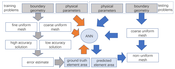
The approach that we propose has a number of components that are not fixed and may be selected by the user. MeshingNet is agnostic about both the mesh generator and the particular FE/FV solver that are used. It is designed to work with existing methods. Furthermore, the a posteriori error can be computed using any user-defined norm (in this paper we consider L1 and energy norms respectively in our two validation tests). Some specific examples of governing equations, geometries, boundary conditions and material parameters are illustrated in the evaluation section. Prior to this however we provide some additional details of the components used in our paper.
2.2 Component Details
Mesh generation. All meshes (LDUM, HDUM and the refined mesh) are created using the software Triangle [19] which conducts Delaunay triangulations. Triangle reads a planar graph, representing the boundary of a two-dimensional polygonal domain as its input and the user may define a single maximum element area across the entire polygon when a uniform mesh is desired. To refine a mesh non-uniformly the user specifies, within each coarse element, what the element area upper bound should be after refinement. Triangle ensures a smooth spatial variation of the element size. The refinement is not nested since, although it does not eliminate the pre-existing vertices of the original mesh, it does break the original edges.
Mesh refinement via error estimation. Broadly speaking, the finer the mesh is, the closer the FE result is expected to be to the ground truth. We regard the HAS as the ground truth by ensuring that HDUMs are always significantly finer than LDUMs. Linear interpolation is used to project the LAS to the fine mesh to obtain LAS*, where LAS* has the same dimension as HAS. An error estimate approximates the error by comparing LAS* and HAS in the selected norm, on the HDUM, and this is then projected back to the original LDUM. The target area upper bound for the refined mesh within each LDUM element is then defined to be inversely correlated with . In this paper, we select as the area upper bound for element number of the LDUM (to be refined), where is the center of the th element, and determines the overall target element number and, in the examples given here, we always choose . By varying appropriately it is possible to adjust the refined mesh to reach a target total number of elements.
MeshingNet model and training. As outlined in subsection 2.1, for a given PDE system, MeshingNet approximates the target local element area upper bound at a given point within a polygonal domain based upon inputs which include: the coordinates of the polygon’s vertices, key parameters of the PDE and the mean value coordinates of the specified point (mean value coordinates, [10], parameterizes a location within a 2D polygon as a convex combination of polygon vertices). Two types of DNNs are considered: a fully connected network (FCN) and two residual networks (ResNets). The dimensions of our FCN layers are X-32-64-128-128-64-32-8-1 (where X represents the dimension of the input and is problem-specific) and each hidden layer uses rectified linear units (ReLU) as the activation function. To further improve and accelerate training, two ResNets are also experimented with to enhance FCN (Fig. 2). ResNet1 enhances FCN by adding a connection from the first hidden layer to the output of the last one. Note that residual connections can help to resolve the vanishing gradient problem in deep networks and improve training [23]. ResNet2 enhances FCN by adding multiple residual connections. This is inspired by recent densely connected convolutional networks [13] which shows superior data-fitting capacity with a relatively small number of parameters. The training data set samples over geometries, BCs and parameter values. Each geometry with fixed BCs and parameters uniquely defines a problem. In a problem, each LDUM element centroid (represented by its mean value coordinates) and its target forms an input-output training pair. We randomly generated 3800 problems of which 3000 are used for training and 800 for testing (because each LDUM contains approximately 1000 elements, there are over 3 million training pairs). We then use stochastic gradient descent, with a batch size 128, to optimize the network. We use mean square error as the loss function and Adam [14] as the optimizer. The implementation is done using Keras [7] on Tensorflow [1] and the training is conducted on a single NVIDIA Tesla K40c graphics card.
Guiding mesh generation via MeshingNet. After training, the network is able to predict the target distribution on a previously unseen polygonal domain. Given a problem, a LDUM is first generated; next, MeshingNet predicts the local target area upper bound, , at the centre, , of the th element; Triangle then refines the LDUM to generate the non-uniform mesh based upon within each element of the LDUM (to be refined). Optionally, this last step may be repeated with an adjusted value of to ensure that the refined mesh has a desired total number of elements (this allows an automated approximation to “the best possible mesh with X elements”).


Error norms. Error estimation provides a means of quantifying both the local and the global error in an initial FE solution. However the precise magnitude and distribution of the error depends on the choice of the norm used to compute the difference between the LAS and the HAS. Different norms lead to different non-uniform meshes. Consequently, for any given PDE system, a single norm should be selected in order to determine from , and (Equation (1)). The appropriate choice of norm is a matter for the user to decide, similar to the choice of specific a posteriori error estimate in the conventional adaptive approach. In the following section two different norms are considered for the purposes of illustration.
3 Validation results
We now assess the performance of MeshingNet through two computational examples: a single PDE, for which we consider only the effect of the domain geometry on the optimal mesh; and a system of PDEs, for which we consider the influence of geometry, BCs and material parameters on the optimal mesh.
3.1 2D Poisson’s equation
We solve Poisson’s equation () on a simply connected polygon with boundary (on which ). The polygons in our data set are all octagons, generated randomly, subject to constraints on the polar angle between consecutive vertices and on the radius being between 100 to 200 (so the polygons are size bounded). The L1 norm relative error estimate is
| (2) |
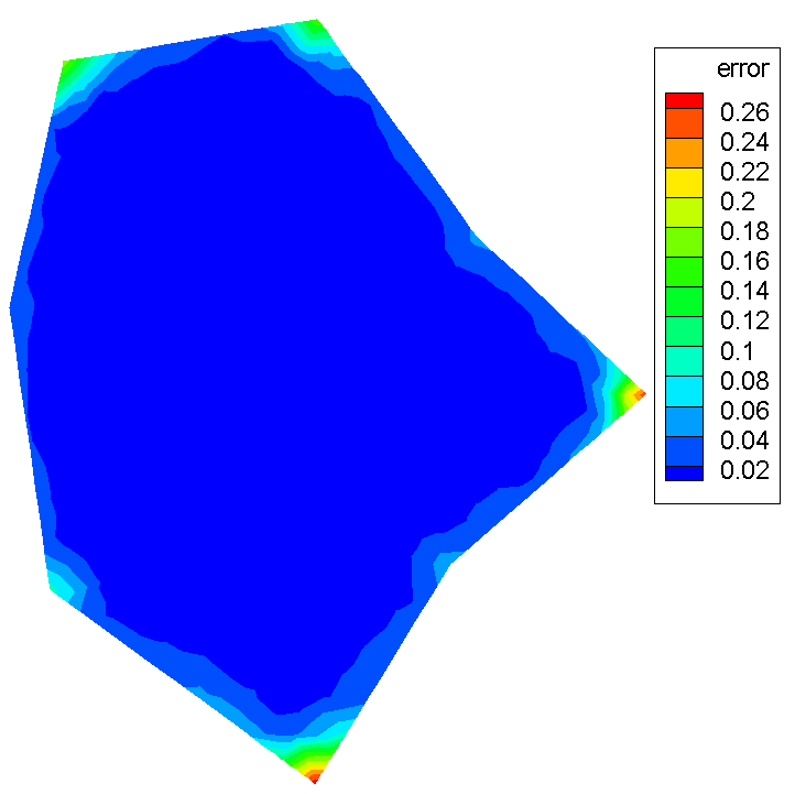
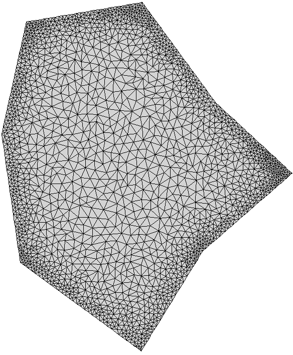
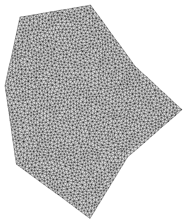
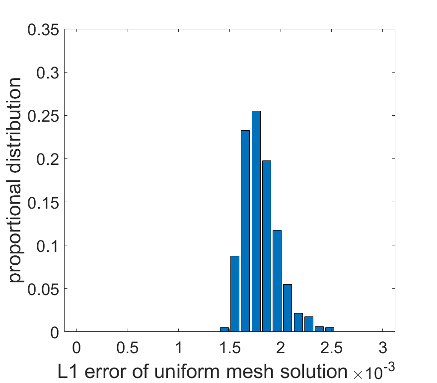
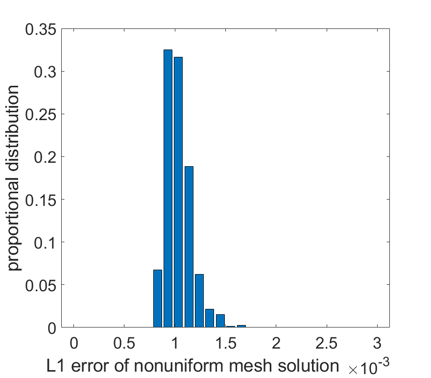
As expected, in Fig. 3 (which shows a typical test geometry), the mesh generated by MeshingNet is dense where the error for the LAS is high and coarse where it is low. Fig. 4 quantifies the improvement of MeshingNet relative to an uniform mesh (Fig. 3 right) by showing, for the entire test data set, the error distributions of the computed FE solutions (relative to the ground truth solutions) in each case.
3.2 2D linear elasticity
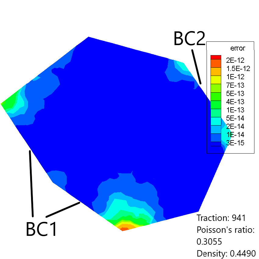
We solve 2D plane stress problems on a set of different polygons (6-8 edges). Each polygon edge is associated with one of three possible BCs. BC1: zero displacement; BC2: uniformly distributed pressure or traction (with random amplitude up to ); and BC3: unconstrained. For different geometries, we number the vertexes and edges anti-clockwise with the first vertex always on the positive x-axis, without loss of generality. To get a combinations of BCs, we always apply BC1 on the first edge, BC2 on the fourth and fifth edges and BC3 on the rest. We also allow different (homogeneous) material properties: density up to a value of and Poisson’s ratio between to . The error approximation uses energy norm
| (3) |
where and are strains of LAS* and HAS, and are stresses of LAS* and HAS. This is the “natural norm” for this problem since the PDEs are the Euler-Lagrange equations for the minimization of the following energy functional:
| (4) |
where is the body force and is the displacement. Due to the linearity of the problem, the relative accuracy of two FE solutions may be determined equivalently by which has the lower error in the energy norm or which has the lower total potential energy (we exploit this in our validation below).
There are 27 dimensions in MeshingNet’s input: 16 for the polygon vertices, 8 for the mean value coordinates of the target point, and 1 each for the traction BC magnitude, density and Poisson’s ratio. We train FCN, Resnet1 and Resnet2 for 50 epochs, each taking 142, 134 and 141 minutes respectively. Fig. 5 shows that the training processes all converge, with ResNet training typically converging faster than FCN. After training, predicting the target (on all LDUM elements) for one problem takes 0.046 seconds on average, which is over 300 times faster than using the a posteriori error method that generates the training data set.
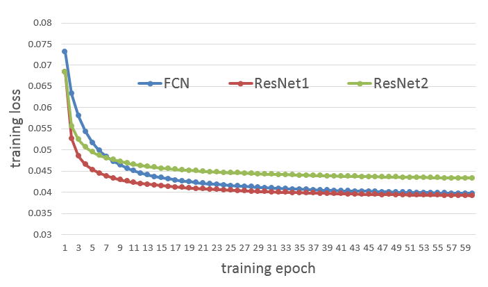
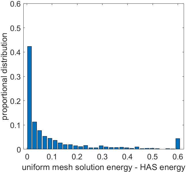
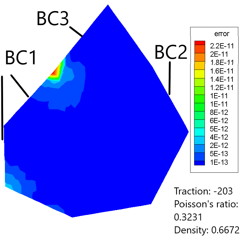
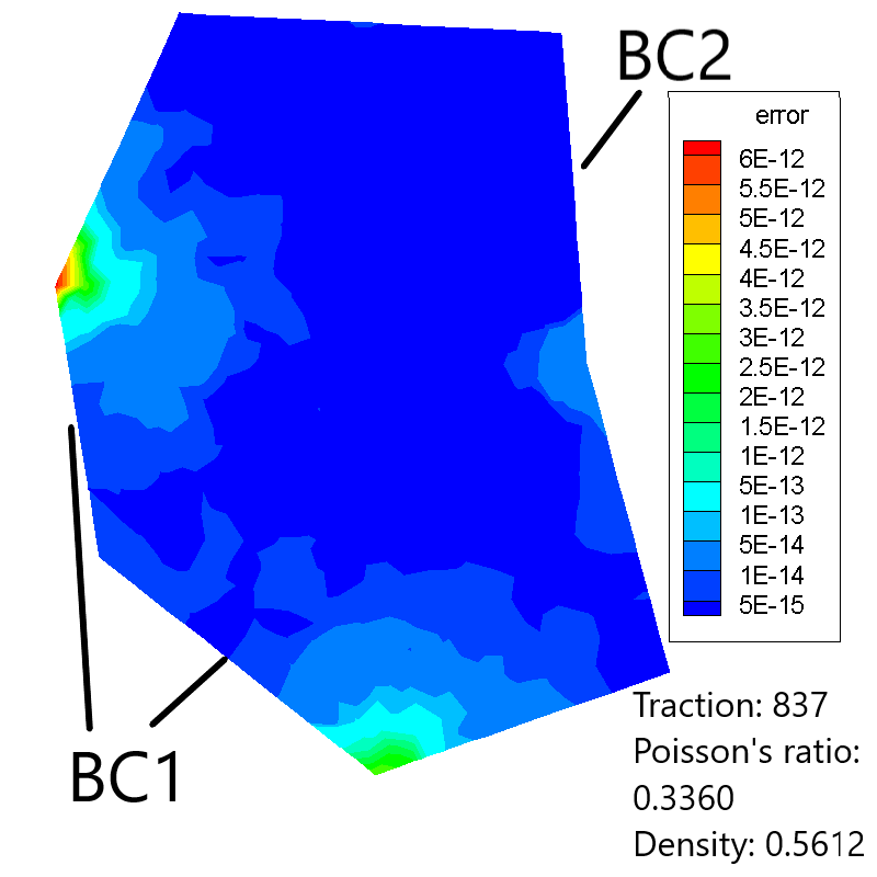
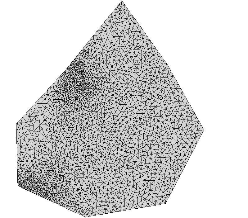
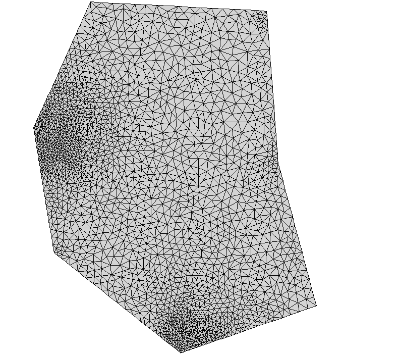
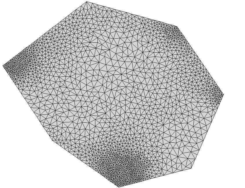
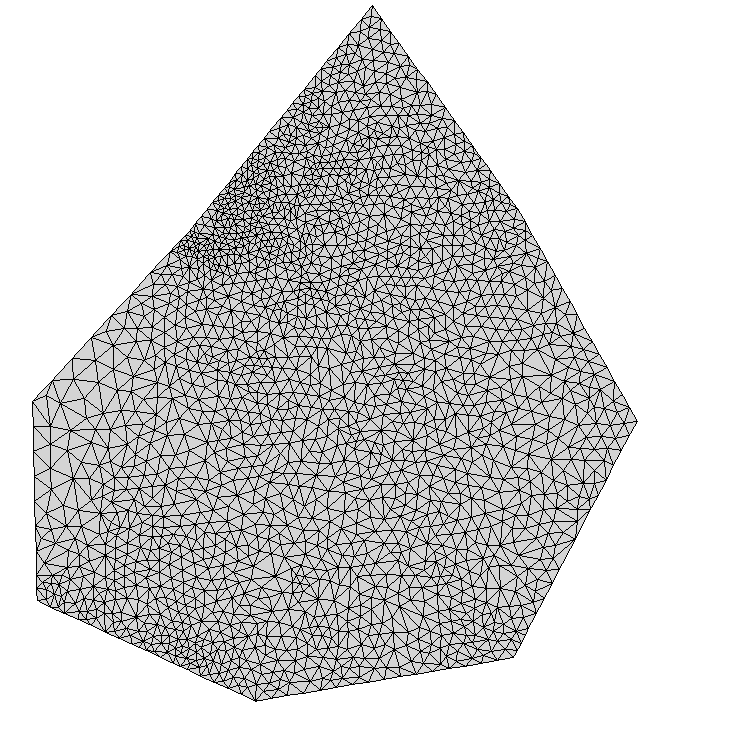
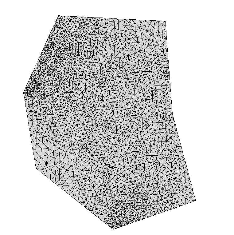
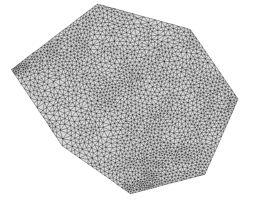
Fig. 6 shows a comparison of FE results computed on MeshingNet meshes, uniform meshes of the same number of elements (4000 elements) and non-uniform meshes (also of the same number of elements) computed based upon local refinement following ZZ error estimation. The former meshes have FE solutions with potential energy significantly lower than the uniform mesh and ZZ refined mesh (and much closer to the HAS potential energy). Fig. 7 illustrates some typical meshes obtained using MeshingNet: the non-uniform meshes correspond to the error distributions in the LAS. Though not shown here due to space constraints, we also find that the traction-to-density ratio impacts the non-uniform mesh most significantly. Overall, this example shows that MeshingNet can generate high quality meshes that not only account for geometry but also the given material properties and BCs.
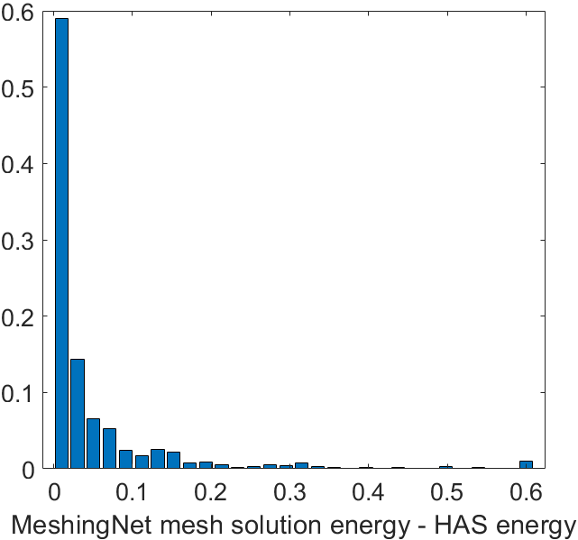
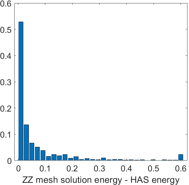
Finally we compare different DNN models, using the average potential energy on the testing data set. The baseline is from the HDUMs, whose FE solutions have a mean energy of , followed by the meshes from ResNet2 (mean energy ), ResNet1 (), and FCN (). The lower the better. These are all far superior to the uniform meshes of the same size (4000 elements), which yield FE solutions with a mean energy of . Note that ResNet not only shortens the training time over FCN but, on average, produces better solutions.
4 Discussion
In this paper, we have proposed a new non-uniform mesh generation method based on DNN. The approach is designed for general PDEs with a range of geometries, BCs and problem parameters. We have implemented a two-dimensional prototype and validated it on two test problems: Poisson’s equation and linear elasticity. These tests have shown the potential of the technique to successfully learn the impact of domain geometries, BCs and material properties on the optimal finite element mesh. Quantitatively, meshes generated by MeshingNet are shown to be more accurate than uniform meshes and non-uniform ZZ meshes of the number of elements. Most significantly, MeshingNet avoids the expense of a posteriori error estimation whilst still predicting these errors efficiently. Even though generating the training data set is expensive, it is offline and is thus acceptable in practice.
The meshes generated via MeshingNet may be used in a variety of ways. If our goal is to obtain a high quality mesh with a desired number of elements then the approach described in this paper provides a cost-effective means of achieving this. If however the goal is to produce a solution with an estimated a posteriori error that is smaller than a desired tolerance, then the generated mesh may not meet this criterion. This may be addressed either by regenerating the mesh based upon a higher target number of elements in the final mesh, or through the use of a traditional a posteriori estimate on the computed solution in order to guide further mesh refinement. In the latter case we can view MeshingNet as a means to obtaining an improved initial mesh within a traditional mesh adaptivity workflow.
In future, we plan to generalize MeshingNet onto more general problems: 3D geometries, more complex PDE systems and BCs (e.g. Navier-Stokes and fluid-structure interactions), and time-dependent cases. For 3D problems, Tetgen [20] is able to do a similar refinement process to what Triangle does in 2D in this paper, which will enable us to directly apply MeshingNet to 3D problems. Furthermore, it would be desirable to develop an interface to enable the mesh generator to read geometries from standard computer aided design software. For complex three-dimensional problems it also seems unlikely that the accurate, but very expensive, approach to training the error estimator that is used in this paper will always be computationally viable (despite its excellent performance). In such cases we may replace this estimator with a more traditional method such as [2, 4, 24], on relatively fine uniform grids for training purposes.
Finally, we note that the ANNs used in this initial investigation are relatively simple in their structure. In the future the use of new DNN models, such as Convolutional/Graph Neural Networks, should be considered. These may be appropriate for problems in three dimensions or with larger data sets, such as arising from more general geometries and boundary conditions.
References
- [1] Abadi, M., et al.: TensorFlow: Large-scale machine learning on heterogeneous systems (2015), http://tensorflow.org/, software available from tensorflow.org
- [2] Ainsworth, M., Oden, J.T.: A posteriori error estimation in finite element analysis. Computer methods in applied mechanics and engineering 142(1-2), 1–88 (1997)
- [3] Apel, T., Grosman, S., Jimack, P.K., Meyer, A.: A new methodology for anisotropic mesh refinement based upon error gradients. Applied Numerical Mathematics 50(3-4), 329–341 (2004)
- [4] Bank, R.E., Weiser, A.: Some a posteriori error estimators for elliptic partial differential equations. Mathematics of computation 44(170), 283–301 (1985)
- [5] Chedid, R., Najjar, N.: Automatic finite-element mesh generation using artificial neural networks-part i: Prediction of mesh density. IEEE Transactions on Magnetics 32(5), 5173–5178 (1996)
- [6] Chen, T.Q., Rubanova, Y., Bettencourt, J., Duvenaud, D.K.: Neural ordinary differential equations. In: Advances in neural information processing systems. pp. 6571–6583 (2018)
- [7] Chollet, F., et al.: Keras. https://keras.io (2015)
- [8] Csáji, B.C.: Approximation with artificial neural networks. Faculty of Sciences, Etvs Lornd University, Hungary 24, 48 (2001)
- [9] Dörfler, W.: A convergent adaptive algorithm for poisson’s equation. SIAM Journal on Numerical Analysis 33(3), 1106–1124 (1996)
- [10] Floater, M.S.: Mean value coordinates. Computer aided geometric design 20(1), 19–27 (2003)
- [11] Grätsch, T., Bathe, K.J.: A posteriori error estimation techniques in practical finite element analysis. Computers & structures 83(4-5), 235–265 (2005)
- [12] Han, J., Jentzen, A., Weinan, E.: Solving high-dimensional partial differential equations using deep learning. Proceedings of the National Academy of Sciences 115(34), 8505–8510 (2018)
- [13] Huang, G., et al.: Densely connected convolutional networks. In: 2017 IEEE Conference on Computer Vision and Pattern Recognition (CVPR). pp. 2261–2269 (July 2017). https://doi.org/10.1109/CVPR.2017.243
- [14] Kingma, D.P., Ba, J.: Adam: A method for stochastic optimization. arXiv preprint arXiv:1412.6980 (2014)
- [15] Krizhevsky, A., Sutskever, I., Hinton, G.E.: Imagenet classification with deep convolutional neural networks. In: Advances in neural information processing systems. pp. 1097–1105 (2012)
- [16] Long, Z., Lu, Y., Ma, X., Dong, B.: Pde-net: Learning pdes from data. arXiv preprint arXiv:1710.09668 (2017)
- [17] Lowther, D., Dyck, D.: A density driven mesh generator guided by a neural network. IEEE transactions on magnetics 29(2), 1927–1930 (1993)
- [18] Notay, Y.: An aggregation-based algebraic multigrid method. Electronic transactions on numerical analysis 37(6), 123–146 (2010)
- [19] Shewchuk, J.R.: Delaunay refinement algorithms for triangular mesh generation. Computational geometry 22(1-3), 21–74 (2002)
- [20] Si, H.: Tetgen, a delaunay-based quality tetrahedral mesh generator. ACM Transactions on Mathematical Software (TOMS) 41(2), 11 (2015)
- [21] Sirignano, J., Spiliopoulos, K.: Dgm: A deep learning algorithm for solving partial differential equations. Journal of Computational Physics 375, 1339–1364 (2018)
- [22] Stevenson, R.: Optimality of a standard adaptive finite element method. Foundations of Computational Mathematics 7(2), 245–269 (2007)
- [23] Veit, A., Wilber, M.J., Belongie, S.: Residual networks behave like ensembles of relatively shallow networks. In: Advances in neural information processing systems. pp. 550–558 (2016)
- [24] Zienkiewicz, O., Zhu, J.: Adaptivity and mesh generation. International Journal for Numerical Methods in Engineering 32(4), 783–810 (1991)