Connecting measurements of solar and stellar brightness variations

Abstract

Context. Comparing solar and stellar brightness variations is hampered by the difference in spectral passbands used in observations as well as by the possible difference in the inclination of their rotation axes from the line of sight.

Aims. We calculate the rotational variability of the Sun as it would be measured in passbands used for stellar observations. In particular, we consider the filter systems used by the CoRoT, Kepler, TESS, and Gaia space missions. We also quantify the effect of the inclination of the rotation axis on the solar rotational variability.

Methods. We employ the Spectral And Total Irradiance REconstructions (SATIRE) model to calculate solar brightness variations in different filter systems as observed from the ecliptic plane. We then combine the simulations of the surface distribution of the magnetic features at different inclinations using a surface flux transport model (SFTM) with the SATIRE calculations to compute the dependence of the variability on the inclination.

Results. For an ecliptic-bound observer, the amplitude of the solar rotational variability, as observed in the total solar irradiance (TSI) is 0.68 mmag (averaged over solar cycles 21-24). We obtained corresponding amplitudes in the Kepler (0.74 mmag), CoRoT (0.73 mmag), TESS (0.62 mmag), Gaia G (0.74 mmag), Gaia G_RP (0.62 mmag), and Gaia G_BP (0.86 mmag) passbands. Decreasing the inclination of the rotation axis decreases the rotational variability. For a sample of randomly inclined stars, the variability is on average 15% lower in all filter systems considered in this work. This almost compensates for the difference in the amplitudes of the variability in TSI and Kepler passbands, making the amplitudes derived from the TSI records an ideal representation of the solar rotational variability for comparison to Kepler stars with unknown inclinations.

Conclusions. The TSI appears to be a relatively good measure of solar variability for comparing with stellar measurements in the CoRoT, Kepler, TESS Gaia G, and Gaia G_RP filters. Whereas the correction factors can be used to convert the amplitude of variability from solar measurements into the values expected for stellar missions, the inclination affects the shapes of the light curves so that a much more sophisticated correction than simple scaling is needed to obtain light curves out of ecliptic for the Sun.

1 Introduction

The dedicated planet-hunting photometric missions such as CoRoT (Convection, Rotation and planetary Transit, see Baglin et al. 2006; Bordé et al. 2003), Kepler (Borucki et al. 2010), and TESS (Transiting Exoplanet Survey Satellite, see Ricker et al. 2014), as well as the Gaia space observatory (Gaia Collaboration 2016) have made it possible to measure stellar brightness variability with unprecedented precision. In particular, they allow studying stellar brightness variations caused by transits (as the star rotates) and the evolution of magnetic features, i.e. bright faculae and dark spots. Such variations are often referred to as rotational stellar variability. The plethora of stellar observational data rekindled an interest in the questions of how typical is our Sun as an active star and, more specifically, how does the solar rotational variability compare to that of solar-like stars? Furthermore, these data allow probing if the solar activity paradigm is valid for other stars as well. This requires comparing the stellar properties and behaviour with those of the Sun. While the solar variability has been measured for over four decades now by various dedicated space missions (see, e.g., Fröhlich 2012; Ermolli et al. 2013; Solanki et al. 2013; Kopp 2016, for reviews), a comparison between solar and stellar brightness measurements is far from straightforward (see, e.g., Basri et al. 2010; Reinhold et al. 2020; Witzke et al. 2020). Firstly, solar and stellar brightness variations have been measured in different spectral passbands. Since the amplitude of the solar rotational variability strongly depends on the wavelength (Solanki et al. 2013; Ermolli et al. 2013), the solar and stellar brightness records can be reliably compared only after conversion from one passband to another. Secondly, the solar brightness variations have (so far) only been measured from the ecliptic plane which is very close to the solar equatorial plane (the angle between the solar equator and ecliptic plane is about 7.25^∘). The values of the angle between the line of sight of the observer and the rotation axes of the observed stars (hereinafter referred to as the inclination) are mostly unknown.

Studies comparing solar and stellar rotational brightness variations have used different types of solar brightness measurements. Reinhold et al. (2020), for instance, used the total solar irradiance (TSI), i.e. the solar radiative flux at 1 AU integrated over all wavelengths. More commonly, however, the solar variability was characterised (see, e.g., Basri et al. 2010; Gilliland et al. 2011; Harrison et al. 2012) using measurements by the Variability of solar IRradiance and Gravity Oscillations / Sun PhotoMeters (VIRGO/SPM) (Fröhlich et al. 1995, 1997) instrument on-board the Solar and Heliospheric Observatory (SoHO). VIRGO/SPM measures solar brightness in three filters with a bandwidth of 5 nm each. Neither VIRGO/SPM nor TSI measurements can be directly compared to records of stellar brightness variability, which typically cover wavelength ranges broader than the VIRGO/SPM filters, but much narrower than the TSI. Therefore accurate estimations of solar variability in passbands used for stellar measurements has so far been missing. Some effort has been already put in the modelling of the solar rotational variability as it would be observed out-of-ecliptic (e.g., Vieira et al. 2012; Shapiro et al. 2016; Nèmec et al. 2020). In particular, Shapiro et al. (2016) and Nèmec et al. (2020) (hereinafter N20) have shown that the amplitude of the solar brightness variations on the rotational timescale decreases with decreasing inclination. Consequently, due to its almost equator-on view, the Sun would appear on average more variable than stars with the same activity level but observed at random inclinations. At the same time, an easy to use receipt for correcting variability for the inclination effect has been missing until now and, consequently, inclination has not yet been quantitatively accounted for in solar-stellar comparison studies.

In this paper we seek to overcome both hurdles and quantify solar variability in passbands used by different stellar space missions and at different inclinations. In Sect. 2 we employ the Spectral And Total Irradiance REconstruction (SATIRE; Fligge et al. 2000; Krivova et al. 2003) model of solar brightness variations to show how the actual solar brightness variations relate to solar brightness variations as they would be observed in spectral passbands used by stellar missions. We also establish the connection between the TSI and VIRGO/SPM measurements. In Sect. 3 we follow the approach developed by N20 to quantify the effect of the inclination on the brightness variations. We discuss, how the Sun as observed by Kepler can be modelled using light curves obtained by VIRGO/SPM in Sect. 4 before we summarise our results and draw conclusions in Sect. 5.

2 Conversion from solar to stellar passbands

2.1 SATIRE-S

The Spectral And Total Irradiance REconstruction (SATIRE, Fligge et al. 2000; Krivova et al. 2003) model attributes the brightness variations of the Sun on timescales longer than a day to the presence of magnetic features, such as bright faculae and dark spots, on its surface. The two main building blocks of SATIRE are the areas and the positions of the magnetic features on the solar disc as well as contrasts of these features relative to the quiet Sun (i.e. regions on the solar surface free from any apparent manifestations of magnetic activity). The contrasts of the magnetic features as a function of disc position and wavelength were computed by Unruh et al. (1999) with the spectral synthesis block of the ATLAS9 code (Kurucz 1992; Castelli & Kurucz 1994). The 1D atmospheric structure of the two spot components (umbra and penumbra) and of the quiet Sun were calculated using radiative equilibrium models produced with the ATLAS9 code, while the facular model is a modified version of FAL-P by Fontenla et al. (1993).

Various versions of the SATIRE model exist. In this section we employ the most precise version, which is SATIRE-S, where the suffix “S” stands for the satellite era Ball et al. (2014); Yeo et al. (2014). SATIRE-S uses the distribution of magnetic features on the solar disc obtained from observed magnetograms and continuum disc images and spans from 1974 to today, covering four solar cycles. As especially the early ground-based observations contain gaps in the data we use the SATIRE-S model as presented by Yeo et al. (2014) (version 20190621), where the gaps in Spectral Solar Irradiance (SSI) and TSI have been filled using the information provided by solar activity indices. SATIRE-S was shown to reproduce the apparent variability of the Sun as observed, in both the SSI and in the TSI (see Ball et al. 2012, 2014; Yeo et al. 2014; Danilovic et al. 2016, and references therein). The spectral resolution of the SATIRE output is 1 nm below 290 nm, 2 nm between 290 nm and 999 nm and 5 nm above 1000 nm. This is fully sufficient for the calculations presented in this study.

2.2 Filter systems

In this section we multiply the SATIRE-S SSI output with the response function of a given filter and integrate it over the entire filter passband to obtain the solar light curve in the corresponding filter. It is important to take the nature of the detectors used in different instruments into account (see e.g. Maxted 2018). In particular, while solar instruments (e.g. VIRGO/SPM and all TSI instruments) measure the energy of the incoming radiation, charge-coupled devices (CCDs) utilised in Kepler, Gaia, and TESS count the number of photons and not their energy. In order to obtain the solar light curve, $LC$, as it would be measured by the instrument counting photons we therefore follow

$$LC=\int\limits_{\lambda_{1}}^{\lambda_{2}}R(\lambda)\cdot I(\lambda)\frac{\lambda}{h\cdot c}\,d\lambda,$$ (1)

where $\lambda_{1}$ and $\lambda_{2}$ are the blue and red threshold wavelengths of the filter passband, $R(\lambda)$ is the response function of the filter and $I(\lambda)$ is the spectral irradiance at a given wavelength, $h$ is the Planck constant, and $c$ the speed of light.

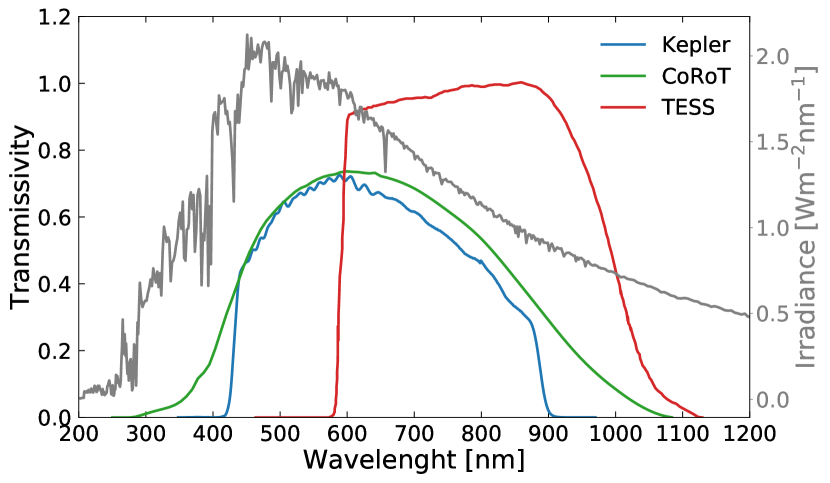
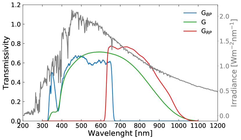
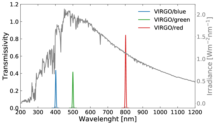
Figure 1: Response functions for the various filter systems used in this study. For comparison, the quiet-Sun spectrum used by SATIRE-S is plotted in grey in each panel. Top panel: Kepler, TESS and CoRoT; middle panel: the three Gaia passbands; bottom panel: the three VIRGO/SPM channels.

First we consider several broad-band filters used by the planetary-hunting missions: CoRoT, Kepler, and TESS. The spectral passbands employed in these missions are shown in the top panel of Fig. 1, along with the quiet-Sun spectrum calculated by Unruh et al. (1999) and used in SATIRE-S. Clearly, the CoRoT and Kepler response functions are very similar to each other, as both missions focused on G-stars. TESS is designed to observe cooler stars compared to Kepler, hence the response function is shifted towards the red part of the spectrum.

Gaia measures stellar brightness in three different channels (Gaia Collaboration 2016). Gaia G is sensitive to photons between 350 and 1000 nm. Additionally, two prisms disperse the incoming light between 330 and 680 nm for the ‘Blue Photometer’ (hereafter, referred to as Gaia G_BP) and between 640–1050 nm for the ‘Red Photometer’ (hereafter, referred to as Gaia G_RP). The response functions are shown in the middle panel in Fig. 1. We employ the revised passbands used for the second data release of Gaia (Gaia DR2, Evans et al. 2018) for the calculations.

Solar-stellar comparison studies have often used the solar variability as it is measured by the VIRGO/SPM instrument. SPM comprises three photometers, with a bandwidth of 5 nm operating at 402 nm (blue), 500 nm (green), and 862 nm (red). The response functions are shown in Fig. 1 in the bottom panel. We refer to these filters from now on simply as VIRGO/blue/green/red.

2.3 Results

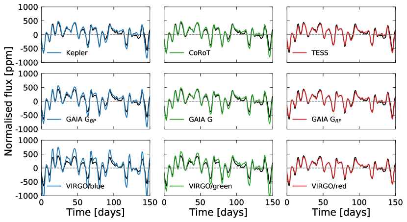
Figure 2: Normalised fluxes for the different filter systems compared to the TSI (black solid line). Top panels: Kepler, CoRoT and TESS, middle panels: the three Gaia passbands, bottom panels : the three VIRGO/SPM channels.

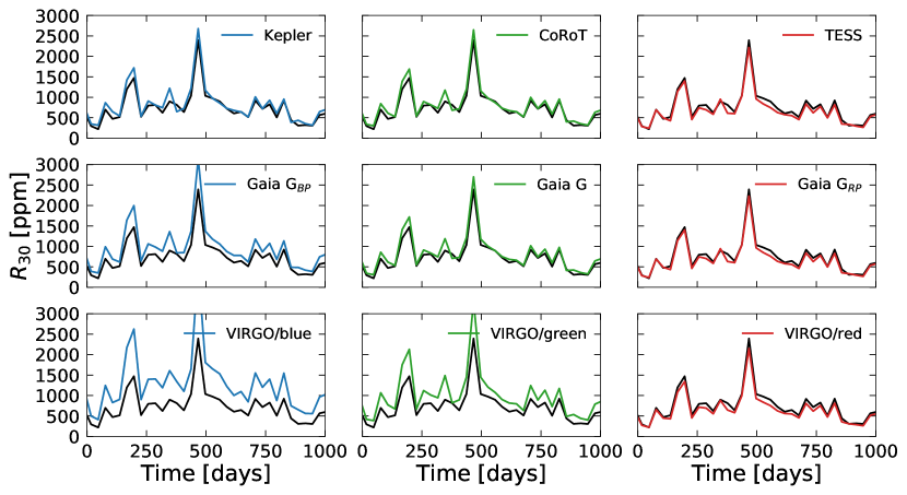
Figure 3: $R_{30}$ in different filter systems compared to the TSI (black solid line) for a timespan of 1000 days over solar cycle 22. Top panels: Kepler, CoRoT and TESS, middle panels: the three Gaia passbands, bottom panels: the three VIRGO/SPM channels. See the main text for the definition of $R_{30}$.

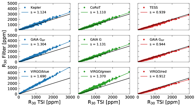
Figure 4: Linear regression between the $R_{30}$-values calculated with the TSI and with the solar light curves as they would be recorded in different filter systems. The values of the slope, $s$, are given in the legend. The black lines have a slope equal to 1.

Figure 2 shows the solar light curve for the period of 2456700 – 2456850 JD (24 February 2014 – 11 July 2014), as it would be observed in different passbands. This corresponds to a 150 –day interval during the maximum of cycle 24. This interval was chosen arbitrarily to display the effect of the filter systems on the solar variability. For this, we first divided each light curve in 90–day segments. This time-span corresponds to Kepler-quarters. This is motivated by the way Kepler observations are gathered and reduced. We note, that the detrending by Kepler operational mode is applied here for purely illustrative purposes and it is not used for calculations presented below. Within each segment, we subtracted the mean value from the fluxes, before dividing the corresponding values by the mean flux in each segment. In all stellar broad-band filters, the light curve turns to be remarkably similar in shape to the TSI (solid black curve), although the amplitude can differ. As one can expect, the difference in the amplitude of the variability is somewhat more conspicuous in the blue filters. The $Gaia\leavevmode\nobreak\ G_{RP}$ light curve is basically identical to the TSI light curve, whereas the variability in $Gaia\leavevmode\nobreak\ G_{BP}$ and in the narrow VIRGO-blue filter show far stronger variability than the TSI.

To quantify the rotational variability, we compute the $R_{30}$ values (see e.g. Basri et al. 2013). For this, the obtained light curves are split into 30-day segments and within each segment, we calculate the difference between the extrema, and divide this value by the mean flux in the segment to get the relative variability. For the SATIRE-S time series we directly consider the difference between the extrema instead of the differences between the 95th and 5th percentiles of sorted flux values, as is usually done in the literature with the more noisy Kepler measurements. We calculate $R_{30}$ values for the period 1974–2019 (i.e. cycles 22–24). This allows us to quantify the mean level of solar variability in $R_{30}$ that represents the full four decades of TSI measurements.

	slope
Kepler	1.123 ($\pm$0.007)
CoRoT	1.110 ($\pm$0.006)
TESS	0.939 ($\pm$0.004)
Gaia GBP	1.304 ($\pm$0.005)
Gaia G	1.131 ($\pm$0.005)
Gaia GRP	0.944 ($\pm$0.004)
VIRGO/blue	1.689 ($\pm$0.003)
VIRGO/green	1.370 ($\pm$0.007)
VIRGO/red	0.912 ($\pm$0.003)

Table 1: Slopes of the linear regressions in Fig. 4.

	21	22	23	24	mean
TSI	0.743	0.806	0.682	0.492	0.681
Kepler	0.808	0.872	0.731	0.530	0.735
CoRoT	0.801	0.866	0.726	0.526	0.730
TESS	0.680	0.739	0.615	0.445	0.620
Gaia GBP	0.944	1.020	0.861	0.625	0.862
Gaia G	0.817	0.883	0.741	0.537	0.744
Gaia GRP	0.684	0.742	0.617	0.447	0.623
VIRGO/blue	1.252	1.352	1.167	0.846	1.154
VIRGO/green	0.983	1.056	0.894	0.653	0.897
VIRGO/red	0.665	0.722	0.600	0.435	0.606

Table 2: Cycle-averaged $R_{30}$ in mmag.

In Fig. 3 we show the $R_{30}$ values for all the filter systems introduced in Sect. 2.2 in comparison to $R_{30}$ of the TSI for a 1000-day interval starting July 26 2013. This interval therefore includes the maximum of solar 24 as well. To better quantify the dependence of $R_{30}$ on the passband, we show linear regressions between the variability $R_{30}$ in each filter system and the TSI in Fig. 4. The slope of the linear regressions are listed in Table 1. The Pearson-correlation coefficient is above 0.98 for all of the filter systems. Naturally, the slope of the linear regressions depends on the considered filter system. For example, TESS and Gaia G regressions have a slope close to 1, but $G_{BP}$ displays a slope >1, whereas VIRGO-red exhibits a slope <1. Unsurprisingly, the slope is highest for the blue VIRGO filter, where the amplitude of the variability is highest. We note that the good agreement of the TSI with the red filters is expected to be valid only for the rotational variability, which is dominated by spots. In contrast, the solar irradiance variability on the activity cycle timescale is given by the delicate balance between facular and spot components and, consequently, has a very sophisticated spectral profile (Shapiro et al. 2016; Witzke et al. 2018). Thus, values of slopes from Table 1 can not be extrapolated from the rotational to the activity cycle timescales (see Shapiro et al. 2016, for the detailed discussion).

Table 2 lists the cycle-averaged values of $R_{30}$ for all passbands in mmag. All in all, Fig. 4, and Tables 1 and 2 show that the TSI is a passable representative for the variability on the solar rotation timescale as it would be observed in the TESS, Kepler, CoRoT, Gaia G, Gaia G_RP and VIRGO-red filters, but it noticeably underestimates the variability in $G_{BP}$, VIRGO-green VIRGO-blue.

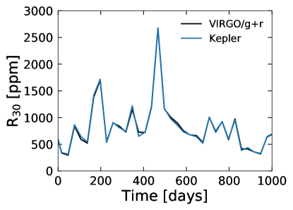
Figure 5: $R_{30}$ over cycle 22 for VIRGO/g+r and Kepler.

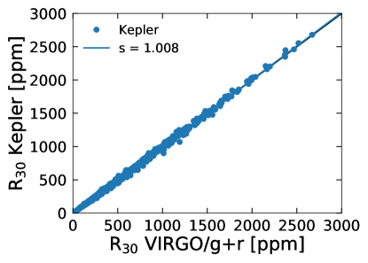
Figure 6: Linear regression between the $R_{30}$ calculated for VIRGO/g+r and for Kepler light curves. The black solid line represents a linear regression with slope $=$ 1.

Several studies (see e.g. Basri et al. 2010; Harrison et al. 2012) have assumed that the amplitude of the rotational solar variability as it would be measured by Kepler is very close to the amplitude calculated for the combined green and red VIRGO/SPM light curves (in the following VIRGO/g+r). Here we test this hypothesis. The variability $R_{30}$ for Kepler in comparison to VIRGO/g+r is shown in Fig. 5, which is limited to the same time interval as Fig. 3. One can see that both curves are remarkably similar to one another. To test the similarity quantitatively, we show the linear regression of $R_{30}$ between Kepler and VIRGO/g+r for four solar cycles (21-24) in Fig. 6. The Pearson correlation coefficient is very high (0.999) and the slope deviates by just +0.8% of unity averaged over four solar cycles. While these calculations relate to the amplitude of the rotational variability, $R_{30}$, we will additionally calculate regressions between Kepler and Virgo light curves in Sect. 4. We also directly connect the TSI and VIRGO/g+r rotational variability. The linear regression between $R_{30}$ in TSI and VIRGO/g+r results in a slope of 0.88 ($\pm$ 0.002) and a Pearson correlation coefficient of 0.995.

3 Correction for the inclination

3.1 Approach

The results presented in Sect. 2.3 are for the Sun viewed from the ecliptic plane and apply to stars that are viewed approximately equator-on. However, this is not always the case and often the inclination of a star is unknown. Calculations of the solar variability as it would be measured by an out-of-ecliptic observer demand information about the distribution of magnetic features on the far-side (for the Earth bound observer) of the Sun. N20 have used a surface flux transport model (SFTM) to obtain the distribution of magnetic features of the solar surface, which was then fed into the SATIRE-model to calculate solar brightness variations as they would be seen at different inclinations.

The SFTM is an advective-diffusive model for the passive transport of the radial magnetic field on the surface of a star, under the effects of large-scale surface flows. In this model, magnetic flux emerges on the stellar surface in the form of bipolar magnetic regions (BMRs). We employ the SFTM in the form given by Cameron et al. (2010) and follow the approach of N20 to simulate light curves of the Sun at different inclinations and with various filter systems. The emergence times, positions and sizes of active regions in our calculations are determined using the semi-empirical sunspot-group record produced by Jiang et al. (2011). This synthetic record was constructed to represent statistical properties of the Royal Greenwich Observatory sunspot record. We additionally randomised the longitudes of the active-region emergences in the Jiang et al. (2011) records. Such a randomisation is needed to ensure that the near- and far-side of the Sun have on average equal activity, which is a necessary condition for reliable calculations of the inclination effect. As a result, our calculations reproduce the statistical properties of a given solar cycle but they do not represent the actual observed BMR emergences for that specific cycle. We stress that in N20 we developed the model outlined above to study the effect of the inclination on the power spectra of solar brightness variations. Here we use this model to study explicitly how the amplitude of the variability on the rotational timescale depends on the inclination in different filters.

3.2 Results

In the following, we displace the observer out of the solar equator towards the solar north pole. This corresponds to inclinations below 90^∘ . We quantify the rotational variability using the $R_{30}$ metric introduced in the previous section. To represent an average level of solar activity, we limit the analysis to cycle 23, which was a cycle of moderate strength.

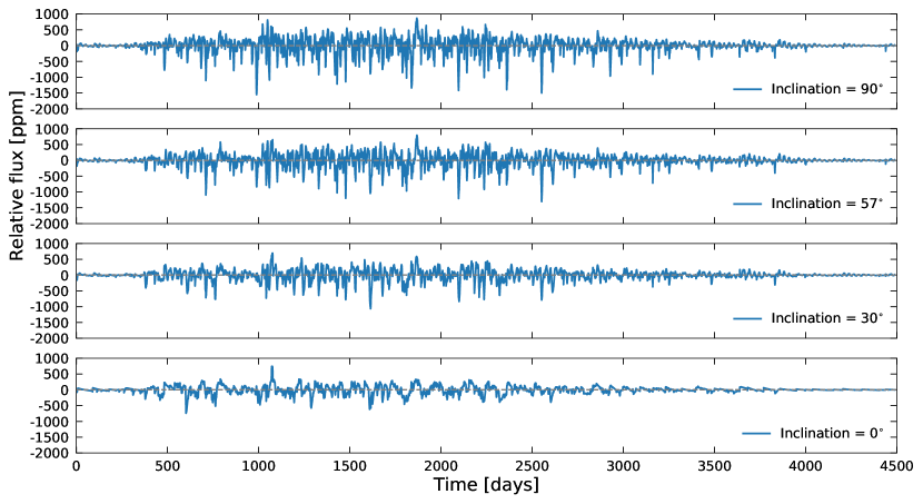
Figure 7: Synthetic solar light curves covering solar cycle 23 in the Kepler passband as it would appear at different inclinations.

Figure 8: Dependence of the mean variability in $R_{30}$ on the inclination (termed $\langle R_{30}\rangle_{\rm i}$, where $i$ stands for the inclination). All values have been normalised to the respective equator-on ($i=90^{\circ}$) value, here called $\langle R_{30}\rangle_{\rm 90}$. Individual curves represent different filter systems. Left panel: Kepler, TESS and CoRoT, middle panel: the three Gaia filters, right panel: the three VIRGO filters and the TSI. The vertical dashed black lines indicates an inclination of 57^∘.

We show the calculated solar light curve as it would be observed by Kepler at various inclinations in Fig. 7. For this, we divided the time-series for cycle 23 in 90-day segments, which correspond to Kepler quarters. Within each quarter, we de-trended the light curves. 90^∘ corresponds to an ecliptic-bound observer, 57^∘ represents a weighted mean value of the inclination with weights equal to the probability of observing a given inclination ($sin(\mathrm{i})$) for the inclination i), and 0^∘ corresponds to an observer facing the north pole. We additionally show 30^∘ as an intermediate point between 57^∘ and 0^∘. For the inclination values of 30^∘, 57^∘, and 90^∘ the variability is brought about by the solar rotation, as well as the emergence and evolution of magnetic features. A polar-bound observer does not observe the rotational modulation, as there is no transit of magnetic features and the variability is merely generated by their emergence and evolution (see Nèmec et al. 2020, for further details). We emphasise just the reduction in the amplitude of the variability with decreasing inclination, but also the change in the shape of the light curve. This is particularly visible in a comparison of the top and the bottom panels of Fig. 7.

In Fig. 8, we show how $R_{30}$ averaged over cycle 23 would change as we displace the observer out of the ecliptic plane. To ease the comparison, we normalised each value of the cycle-averaged variability, $\langle R_{30}\rangle_{\rm i}$, to the corresponding value for the ecliptic view, $\langle R_{30}\rangle_{\rm 90}$. Figure 8 shows that the rotational variability decreases monotonically with decreasing inclination. This trend is seen across all considered filter systems. The differences in the inclination effect among the filter systems are due to the different dependencies of the facular and spot contrasts (as well as their centre-to-limb variations) on the wavelengths.

To evaluate the averaged effect of the inclination, we introduce a new measure that we call $\langle R_{30}\rangle$ and define as

$$\langle R_{30}\rangle=\frac{\sum_{i}\langle R_{30}\rangle_{i}\cdot\mathrm{sin}(i)}{\sum_{i}\mathrm{sin}(i)},$$ (2)

where $i$ is the inclination. The factor $\mathrm{sin}(i)$ ensures that the corresponding values of $\langle R_{30}\rangle_{i}$ are weighted according to the probability that a star is observed at inclination $i$. The $\langle R_{30}\rangle$ value represents the variability of the Sun averaged over all possible inclinations. In other words, if we observed many stars analogous to the Sun with random orientations of the rotation axes, their mean variability would be given by the $\langle R_{30}\rangle$ value. Therefore $\langle R_{30}\rangle$ should be used for the solar-stellar comparison rather than the $\langle R_{30}\rangle_{90}$ value.

We present $\langle R_{30}\rangle$ normalised to $\langle R_{30}\rangle_{90}$ for all considered filter systems as well as the $\langle R_{30}\rangle$ values themselves in Table 3. In the second column of Table 3 we give the inclination-corrected value of the mean rotational variability from Table 2 for easier application of our results. On average, all filter systems show 15% less variability compared to the equatorial case. This implies that the slopes of the linear regressions between the $R_{30}$ values in different passbands and the TSI have to be corrected for the inclination. When comparing stellar measurements in the Kepler passband with the TSI records this means the following: if stars are observed from their equatorial planes, the variability in Kepler is about 12% higher than in the TSI (see the slope given in Table 1). However, when comparing the Sun to a group of stars with random orientations of rotation axes the inclination effect must be taken into account as well. It will reduce stellar variability observed in Kepler passband by approximately 15%. Coincidentally, both effects almost exactly cancel each other and the observed TSI variability appears to be a very good metric for the solar-stellar comparison of Kepler stars in a statistical sense.

	$\langle R_{30}\rangle$/$\langle R_{30}\rangle_{90}$ [%]	$\langle R_{30}\rangle$ [mmag]
TSI	85.1	0.58
Kepler	84.8	0.62
CoRoT	83.8	0.61
TESS	84.0	0.56
Gaia GBP	83.7	0.72
Gaia G	84.1	0.62
Gaia GRP	84.9	0.52
VIRGO/blue	83.9	0.98
VIRGO/green	85.3	0.76
VIRGO/red	83.4	0.50

Table 3: $\langle R_{30}\rangle$/$\langle R_{30}\rangle_{90}$ and $\langle R_{30}\rangle$ values for different filter systems. For $\langle R_{30}\rangle$ we multiplied $\langle R_{30}\rangle$/$\langle R_{30}\rangle_{90}$ by the corresponding value for $\langle R_{30}\rangle_{90}$ from Table 2. Time averaging is performed over the solar cycle 23.

We have shown in Sect. 2 that the amplitude of solar rotational variability as it would be measured by Kepler can be very accurately approximated by calculating the amplitude of the VIRGO/g+r light curve. However, when comparing brightness variations of the Sun to those of a large group of stars with unknown inclinations, one should use solar variability averaged over all possible inclinations rather than solar variability observed from the ecliptic plane. We have established that the effect of a random inclination decreases the variability in the Kepler passband by 15%. Taking this into account, the relative difference between the variability in VIRGO/g+r and the solar variability in Kepler averaged over inclinations is $-14$%. Unlike for the TSI, corrections for the passband and the inclination only partly compensate each other. We therefore suggest that the TSI is a better representative of the Sun as it would be observed by Kepler than VIRGO/g+r, if the inclination of a star is unknown.

4 Modelling Kepler light curves using VIRGO/SPM

The the previous sections, we have quantitatively validated the argument of Basri et al. (2010) that the VIRGO/g+r light curve correspond to the same variability as the Kepler light curve if both light curves are recorded from the solar equatorial plane. In this section we perform complementary calculations. Namely, we test if the Kepler light curve can be modelled as a linear combination of solar light curves in the different VIRGO/SPM channels. We restrict our calculations to solar cycle 23. All light curves are computed with the N20 model.

We divide all light curves into 90-day segments and calculate the relative flux within these segments (i.e. we consider the same normalisation of light curves as shown in Figs. 2 and 7). Next, we apply multiple linear regression to fit the Kepler light curve with the VIRGO/SPM/green+red light curves, to find the best set of coefficients for the linear fit.

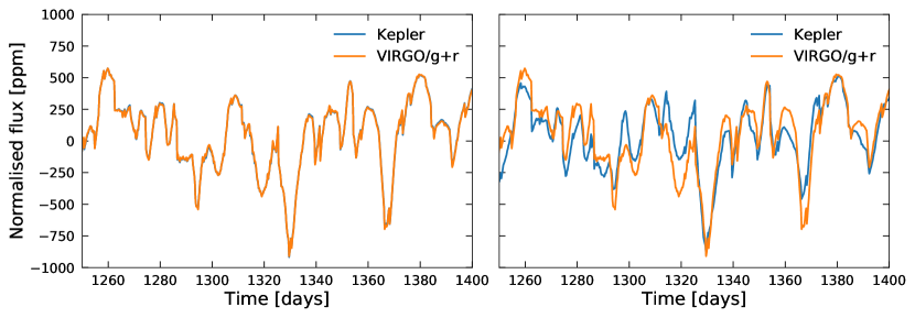
Figure 9: Comparison between the Kepler and the regressed VIRGO/green+red light curve. Left:i = 90^∘, right:i=57^∘. For the coefficients of the fit, see text.

For an ecliptic-bound observer we write the multiple linear regression in the form

$$K_{i,\,SPM}=a\cdot V_{g}+b\cdot V_{r},$$ (3)

where $i$ is the inclination, $V_{g}$ and $V_{r}$ are solar light curves in VIRGO/SPM blue green and red filters (corresponding to the equatorial plane). The best fit for $i=90^{\circ}$ yields a$=$0.275 ($\pm$ 0.001) and b$=$0.619 ($\pm$ 0.002). The $r^{2}$-value is 0.999. Such a high correlation is not surprising giving the similarity between the VIRGO/SPM and Kepler rotational variability discussed in Sect. 2. Next, we apply the multiple-regression model to simulate the out-of-ecliptic Kepler-like light curve using the light curves in the SPM channels as the input. Given that an inclination of 57^∘ is often used to represent a statistical mean of all possible inclination values, we fit the Kepler light curve observed at $i=57^{\circ}$ with a linear combination of VIRGO light curves (observed at $i=90^{\circ}$). The best fit results in the following coefficients: a$=-$0.421 ($\pm$ 0.018) and b$=$1.418 ($\pm$ 0.027), with $r^{2}=0.83$.

Figure 9 compares the Kepler-like light curve with the regression model using light curves in all three VIRGO filters for $i=90^{\circ}$ and $i=57^{\circ}$. For the 90^∘ inclination case (left panel in Fig. 9), the differences between the two light curves are basically invisible, but for the 57^∘ case, the differences are quite pronounced. These differences have various origins. In particular, the transits of magnetic features would take different times for the ecliptic and out-of-ecliptic observer. Furthermore, with decreasing inclination, the facular contribution becomes stronger, while the spot contribution weakens (see e.g., Shapiro et al. 2016), changing the shape of the light curve. It is therefore necessary to take the actual distribution of magnetic features into account when modelling light curves observed at different inclination angles.

5 Conclusions

In this study we give recipes how to treat two problems hindering the comparison between solar and stellar rotational brightness variations: the difference between the spectral passbands utilised for solar and stellar observations as well as the effect of inclination.

To quantify the effect of different spectral passbands on the rotational variability represented through the $R_{30}$ metric, we employed the SATIRE-S model. We found that the rotational variability observed through the filter systems used by the Kepler and CoRoT missions is around 12% higher than the TSI, whereas the variability in the TESS passband is about 7% lower. For Gaia G we find +15% and for Gaia G_BP +30% difference in the amplitude of the rotational variability compared to the TSI, whereas Gaia G_RP shows a difference of -7%. These numbers are valid for equator-on observations on rotational timescales.

Previous studies have used combinations of the green and VIRGO red light curves for solar-stellar comparisons (see e.g. Basri et al. 2010; Gilliland et al. 2011; Harrison et al. 2012). We used linear regressions of the rotational variability between the two combined VIRGO/SPM passbands and the solar variability as Kepler would observe it, to test the goodness of that comparison. We find that the variability in Kepler is 7% higher compared to that of VIRGO/green+red. Moreover, we found that the sum of the VIRGO green and red light curves very accurately represents the solar light curve in the Kepler passband. This is valid, however, only valid for the Sun observed from the ecliptic. We show that a linear combination of VIRGO/SPM passbands cannot accurately reproduce the solar Kepler light curve observed out-of-ecliptic.

We have calculated the dependence of the rotational variability on inclination by following the approach in Nèmec et al. (2020). In this approach, an SFTM is used to simulate the distribution of magnetic features on the surface of the Sun, which is then used to compute the brightness variations with SATIRE. We find that across all filter systems discussed in this study the rotational variability drops by about 15% when it is averaged over all possible directions of the rotation axis. Given that the Kepler rotational variability as observed from the ecliptic plane is 12% higher than the TSI rotational variability, we conclude, that the TSI is the best proxy for the solar rotational brightness variations if they would be observed by Kepler when the inclination effect is considered.