A Sensitivity Matrix Based Methodology for Inverse Problem Formulation

Abstract

We propose an algorithm to select parameter subset combinations that can be estimated using an ordinary least-squares (OLS) inverse problem formulation with a given data set. First, the algorithm selects the parameter combinations that correspond to sensitivity matrices with full rank. Second, the algorithm involves uncertainty quantification by using the inverse of the Fisher Information Matrix. Nominal values of parameters are used to construct synthetic data sets, and explore the effects of removing certain parameters from those to be estimated using OLS procedures. We quantify these effects in a score for a vector parameter defined using the norm of the vector of standard errors for components of estimates divided by the estimates. In some cases the method leads to reduction of the standard error for a parameter to less than 1% of the estimate.

Keywords: Inverse problems, ordinary least squares, sensitivity matrix, Fisher Information matrix, parameter selection, standard errors.

AMS Classification: 34A55, 93E24, 49Q12, 62F07, 62H12, 62G08.

Acknowledgments: A.C.-A. is grateful to Dr. Sava Dediu for helpful discussions about sensitivity identifiability that led to the initial version of this manuscript. This research was supported in part by Grant Number R01AI071915-07 from the National Institute of Allergy and Infectious Diseases and in part by the Air Force Office of Scientific Research under grant number FA9550-09-1-0226. The content is solely the responsibility of the authors and does not necessarily represent the official views of the NIAID, the NIH or the AFOSR.

1 Introduction

The question of parameter identifiability/estimation in the context of parameter determination from system observations or output is at least forty years old and received much attention in the zenith years of linear system and control theory in the investigation of observability, controllability and detectability [3, 9, 10, 22, 23, 28, 30, 34, 36]. These early investigations and results were focused primarily on engineering applications, but much interest in other areas (e.g, oceanography, biology) has prompted more recent inquiries for both linear and nonlinear dynamical systems [2, 8, 18, 21, 26, 32, 41, 43, 44, 45]. In some of the earliest results, Bellman and Astrom [9] defined the concept of structural identifiability, and provided a theoretical framework to address, a priori, whether or not it is possible to determine estimates of unknown parameters from experimental data. Specifically they showed that controllablility (in the sense of the Kalman [28] controllability matrix possessing full rank) implies identifiability, thereby establishing one of the earliest linear algebraic tests for identifiability. In another important early linear algebraic effort, Reid [34] defined the term sensitivity identifiability . If $\displaystyle z(\theta)$ denotes the output of a model depending on a parameter vector $\displaystyle\theta$, then Reid explains sensitivity identifiability in the following way. Let $\displaystyle\Delta\theta$ denote a local perturbation about a nominal $\displaystyle\theta_{0}$, i.e., $\displaystyle\Delta\theta=\theta-\theta_{0}$, which gives rise to local (small) perturbation $\displaystyle\Delta z$ in the output, i.e., $\displaystyle\Delta z=z(\theta)-z(\theta_{0})$. Suppose that $\displaystyle\chi=\frac{\partial z}{\partial\theta}$ denotes the sensitivity matrix, i.e., the Jacobian matrix of the output, being evaluated at $\displaystyle\theta_{0}$ [4, 6]. Then the first order Taylor approximation (exact for linear dependence on the parameter)

$$\Delta z\approx\chi\Delta\theta.$$ (1)

relates the perturbations. A parameter vector is defined as sensitivity identifiable if equation (1) can be solved uniquely (in the local sense) for $\displaystyle\Delta\theta$ [18, 34]. In their review, Cobelli and DiStefano [18] explain that a sufficient condition for sensitivity identifiability is the nonsingularity of the matrix $\displaystyle\chi^{T}\chi$ or equivalently

$$\det(\chi^{T}\chi)\neq 0.$$

From this one sees immediately that parameter estimation depends inherently on the condition number of the Fisher Information Matrix (FIM) $\displaystyle F=\chi^{T}\chi$. Not surprisingly, subsequent investigations of parameter estimation (in applied mathematics, engineering, and statistics) have focused on the role of the FIM. It is now well known that this matrix and its condition number play a fundamental role in a range of useful ideas such as model comparison [12] (the Akaike Information Criteria, the Takeuchi Information Criteria, etc.), generalized sensitivity functions [6, 7, 40] and experimental design (duration, frequency, quality, etc., of observations required to reliably estimate parameters) as well as computation of standard errors and confidence intervals [4, 5, 7, 19].

Brun, et al., [11] and Burth, et al., [13] proposed analyses that use submatrices of the FIM $\displaystyle\chi^{T}\chi$. Burth, et al., implement a reduced-order estimation by determining which parameter axes lie closest to the ill-conditioned directions of $\displaystyle\chi^{T}\chi$, and then by fixing the associated parameter values at prior estimates throughout an iterative estimation process. Brun, et al., determined identifiability of parameter combinations using the eigenvalues of submatrices that result from only using some columns of $\displaystyle\chi^{T}\chi$. Motivated by these efforts and those on the relationship between ill-conditioning of the FIM and quality of parameter estimates investigated in [5, 6, 7], we here use the sensitivity matrix $\displaystyle\chi$ to develop a methodology to assist one in parameter estimation or inverse problem formulations.

In particular, in this paper we investigate the problem of finding multiple solutions for unknown parameters from observations with a statistical error structure (a more practical setting than one assuming noise free observations). We address parameter identifiability by exploiting properties of both the sensitivity matrix and uncertainty quantifications in the form of standard errors. We propose an algorithm inspired by [11, 13], to select parameter combinations (vectors) in two stages. In the first stage, all possible parameter combinations (i.e., subsets of all parameters) are considered and only those with a full rank sensitivity matrix are selected. In the second stage, a score involving uncertainty quantification (standard errors) is calculated for each parameter vector selected in the first stage. Then parameter subset combinations are examined in view of their score and the condition number of corresponding sensitivity matrices. We believe that some form of this type of practical identifiability analysis could be carried out a priori, i.e., before any attempt to solve inverse problems (from experimental observations) is made. We illustrate the ideas and methodology with a seasonal epidemic model.

This manuscript is organized in the following manner. Section 2 introduces the seasonal epidemic model. In Section 3 we explain the statistical model for the observation process; we define the ordinary least squares (OLS) estimator and define precisely the Fisher information matrix. Using a first order Taylor expansion of the model output we compute the OLS estimator in terms of the sensitivity matrix singular values and the error in the observation process. Section 4 contains the proposed subset selection algorithm. In Section 5 some illustrations of the algorithm are discussed, in light of using both synthetic and observational data sets. We conclude with a brief discussion in the last section.

2 Motivating seasonal SEIRS model with demography

We introduce a specific model, a standard Susceptible-Exposed-Infective-Recovered-Susceptible (SEIRS) model, to illustrate the methodology we discuss in this paper. In particular we consider a seasonal model for disease spread and progression in a population. Seasonal patterns of disease incidence are observed in epidemics of influenza [20], meningococcal meningitis [35], measles [1], and rubella [42], to mention a few. Many temporal factors play a role in the formation of cyclical patterns, for instance [25]: (i) survival of the pathogen outside the host, (ii) host behavior and (iii) host immune function.

Cyclical incidence patterns are often modeled with a transmission parameter being a function of time. We denote the time-dependent transmission parameter by $\displaystyle\beta(t)$; it is traditionally defined by [20, 27]

$$\beta(t)=\beta_{0}\left[1+\beta_{1}\cos(2\pi(t-t_{0}))\right],$$ (2)

where $\displaystyle\beta_{0}$ is called the baseline level of transmission, $\displaystyle\beta_{1}$ is known as the amplitude of seasonal variation or simply the strength of seasonality, and $\displaystyle t_{0}$ denotes the transmission parameter phase shift. We may, for convenience, derive an equivalent formulation. Because

$$\beta_{1}\cos(2\pi(t-t_{0}))=a_{1}\cos(2\pi t)+b_{1}\sin(2\pi t),$$

where $\displaystyle a_{1}=\beta_{1}\cos(2\pi t_{0})$ and $\displaystyle b_{1}=\beta_{1}\sin(2\pi t_{0})$, we may re-write equation (2) as

$$\beta(t)=\beta_{0}\left(1+a_{1}\cos(2\pi t)+b_{1}\sin(2\pi t)\right).$$ (3)

The time-dependent transmission parameter $\displaystyle\beta(t)$, as defined in equation (3), is used in the seasonal epidemic model introduced here. Four main epidemiological events are described: latent infection, active infection, recovery, and loss of immunity. It is assumed that individuals becoming infected undergo latency, a period of time during which they are incapable of effectively transmitting the infectious agent, before progressing into active infection. People recover from active infection and develop temporary immunity (they will eventually become susceptible once again). Four epidemiological classes are considered, and at time $\displaystyle t$ the number of: susceptible is denoted by $\displaystyle S(t)$; latent or exposed is denoted by $\displaystyle E(t)$; infectious is denoted by $\displaystyle I(t)$; and recovered or temporarily immune is denoted by $\displaystyle R(t)$. The nonlinear differential equations [29, 39]

$$\displaystyle\frac{dS}{dt} \displaystyle= \displaystyle\frac{1}{P}N+\frac{1}{L}R(t)-\beta(t)S(t)\frac{I(t)}{N}-\frac{1}{P}S(t)$$ (4)

$$\displaystyle\frac{dE}{dt} \displaystyle= \displaystyle\beta(t)S(t)\frac{I(t)}{N}-\frac{1}{M}E(t)-\frac{1}{P}E(t)$$ (5)

$$\displaystyle\frac{dI}{dt} \displaystyle= \displaystyle\frac{1}{M}E(t)-\frac{1}{D}I(t)-\frac{1}{P}I(t)$$ (6)

$$\displaystyle\frac{dR}{dt} \displaystyle= \displaystyle\frac{1}{D}I(t)-\frac{1}{L}R(t)-\frac{1}{P}R(t)$$ (7)

$$\displaystyle N \displaystyle= \displaystyle S(t)+E(t)+I(t)+R(t)$$ (8)

$$\displaystyle S(t_{0}) \displaystyle= \displaystyle S_{0}$$ (9)

$$\displaystyle E(t_{0}) \displaystyle= \displaystyle E_{0}$$ (10)

$$\displaystyle I(t_{0}) \displaystyle= \displaystyle I_{0}$$ (11)

$$\displaystyle R(t_{0}) \displaystyle= \displaystyle N-S_{0}-E_{0}-I_{0},$$ (12)

define the epidemic dynamics known as an SEIRS model. This formulation takes into account demographic processes (the birth rate is $\displaystyle N/P$ and the average life span is $\displaystyle P$) while assuming the total population size $\displaystyle N$ remains constant.

The mean latency period is denoted by $\displaystyle M$, while the average length of active infection is denoted by $\displaystyle D$. It is also assumed immunity lasts an average of $\displaystyle L$ units of time.

In this paper we consider a scenario where the initial conditions of the SEIRS model ($\displaystyle S_{0}$, $\displaystyle E_{0}$, and $\displaystyle I_{0}$) may be unknown, and may need to be estimated, along with all the other model parameters. We apply inverse problem methodologies to determine estimates of the vector parameter

$$\theta=(S_{0},E_{0},I_{0},N,L,D,M,P,\beta_{0},a_{1},b_{1})^{T}\in\mathbb{R}^{p}=\mathbb{R}^{11},$$ (13)

according to an ordinary least squares criterion (defined in the next section).

3 Statistical model for the observation process

The observation process is formulated assuming the SEIRS model, together with a particular choice of parameters (the “true” parameter vector denoted as $\displaystyle\theta_{0}$) describes the epidemic process exactly, but that the $\displaystyle n$ longitudinal observations $\displaystyle\left\{Y_{j}\right\}_{j=1}^{n}$ are affected by random deviations (such as measurement errors) from this underlying process. More precisely, if $\displaystyle z(t_{j};\theta_{0})$ denotes the number of new cases of active infection (also referred to as the model output) between the observation time points $\displaystyle t_{j-1}$ and $\displaystyle t_{j}$, which is defined as

$$z(t_{j};\theta_{0})=\int_{t_{j-1}}^{t_{j}}\frac{1}{M}E(t;\theta_{0})dt,$$ (14)

then the statistical model for the observation process is

$$\displaystyle Y_{j}=z(t_{j};\theta_{0})+\mathcal{E}_{j} \displaystyle\mbox{ for }j=1,\dots,n.$$ (15)

The errors $\displaystyle\mathcal{E}_{j}$ are assumed to be random variables satisfying the following assumptions:

• the errors $\displaystyle\mathcal{E}_{j}$ have mean zero: $\displaystyle E[\mathcal{E}_{j}]=0$;

• the errors $\displaystyle\mathcal{E}_{j}$ have finite common variance: $\displaystyle\mbox{var}(\mathcal{E}_{j})=\sigma_{0}^{2}<\infty$;

• the errors $\displaystyle\mathcal{E}_{j}$ are independent (i.e., $\displaystyle\mbox{cov}(\mathcal{E}_{j},\mathcal{E}_{i})=0$ whenever $\displaystyle j\neq i$) and identically distributed.

Under these assumptions, we have that the mean of the observation equals the model output: $\displaystyle E[Y_{j}]=z(t_{j};\theta_{0})$ and the variance in the observations is constant in time: $\displaystyle\mbox{var}(Y_{j})=\sigma_{0}^{2}$.

3.1 Ordinary least squares (OLS)

We consider an ordinary least squares (OLS) formulation of a generic parameter estimation or inverse problem for a vector parameter ($\displaystyle\theta$) dependent system

$$\displaystyle\frac{dx}{dt}(t) \displaystyle=g(t,x(t;\theta);\theta),$$ (16)

$$\displaystyle x(t_{0}) \displaystyle=x_{0}$$ (17)

with observation (or model output) process

$$z(t_{j})=\mathcal{F}(x(\cdot),\theta),\quad j=1,\dots,n.$$ (18)

In this context we consider a given vector of observations $\displaystyle Y=(Y_{1},\dots,Y_{n})^{T}$, where each $\displaystyle Y_{j}$ is defined by equation (15), and the model output vector $\displaystyle z(\theta)=(z(t_{1};\theta),\dots,z(t_{n};\theta))^{T}$ for a given $\displaystyle\theta$. The estimator $\displaystyle\theta_{OLS}=\theta_{OLS}^{n}$ is a random variable that minimizes the Euclidian norm (in $\displaystyle\mathbb{R}^{n}$ ) square of $\displaystyle Y-z(\theta)$, i.e., $\displaystyle\theta_{OLS}^{n}$ minimizes

$$J(\theta|Y)\equiv\left|Y-z(\theta)\right|^{2}=\left[Y-z(\theta)\right]^{T}\left[Y-z(\theta)\right]=\sum_{j=1}^{n}\left[Y_{j}-z(t_{j};\theta)\right]^{2},$$ (19)

which implies $\displaystyle\theta_{OLS}$ solves the gradient equation

$$\nabla_{\theta}(\left|Y-z(\theta)\right|^{2})=0.$$ (20)

Asymptotic theory can be used to describe the distribution of the estimator $\displaystyle\theta_{OLS}$ [4, 19, 37]. Provided that a number of regularity conditions as well as sampling conditions are met (see [37] for details), it can be shown that, asymptotically (i.e., as $\displaystyle n\rightarrow\infty$), $\displaystyle\theta_{OLS}$ is approximately distributed according to a multivariate normal distribution, i.e.,

$$\theta_{OLS}^{n}\sim\mathcal{N}_{p}\left(\theta_{0},\Sigma_{0}^{n}\right),$$ (21)

where $\displaystyle\Sigma_{0}^{n}=\sigma^{2}_{0}[n\Omega_{0}]^{-1}\in\mathbb{R}^{p\times p}$ and

$$\Omega_{0}=\lim_{n\rightarrow\infty}\frac{1}{n}\chi^{n}(\theta_{0})^{T}\chi^{n}(\theta_{0}).$$ (22)

We remark that the theory requires that this limit exists and that the matrix $\displaystyle\Omega_{0}$ be non-singular. The matrix $\displaystyle\Sigma_{0}^{n}$ is the $\displaystyle p\times p$ covariance matrix $\displaystyle\mbox{cov}\left((\theta_{OLS}^{n})_{i},(\theta_{OLS}^{n})_{j}\right)$, and the $\displaystyle n\times p$ matrix $\displaystyle\chi(\theta_{0})\equiv\chi^{n}(\theta_{0})$ is called the sensitivity matrix of the system, and its $\displaystyle j$th row is equal to $\displaystyle\nabla_{\theta}z(t_{j};\theta_{0})$. More precisely,

$$\displaystyle\chi_{ji}^{n}(\theta_{0})=\left.\frac{\partial z(t_{j};\theta)}{\partial\theta_{i}}\right|_{\theta=\theta_{0}} \displaystyle 1\leq j\leq n,\ 1\leq i\leq p.$$ (23)

For the motivating SEIRS model, the partial derivatives of the state variable vector $\displaystyle x=(S,E,I,R)^{T}$ with respect to $\displaystyle\theta$ can be readily calculated. If $\displaystyle g=(g_{1},g_{2},g_{3},g_{4})^{T}$ denotes the vector function whose entries are given by the expression on the right sides of equations (4)–(7), then we can write the seasonal SEIRS model in the general vector form (16). The sensitivities $\displaystyle\partial x/\partial\theta$ are calculated, for a given $\displaystyle\theta=\hat{\theta}_{OLS}$ (defined below), by solving (see [4, 17] and the references therein) equation (16) and then

$$\displaystyle\frac{d}{dt}\frac{\partial x}{\partial\theta} \displaystyle= \displaystyle\frac{\partial g}{\partial x}\frac{\partial x}{\partial\theta}+\frac{\partial g}{\partial\theta},$$ (24)

from $\displaystyle t=t_{0}$ to $\displaystyle t=t_{n}$. In equation (24) the matrix $\displaystyle\partial g/\partial x$ is $\displaystyle 4\times 4$, while the matrices $\displaystyle\partial x/\partial\theta$ and $\displaystyle\partial g/\partial\theta$ are $\displaystyle 4\times p$.

The solution of equation (20) obtained using a realization $\displaystyle y=(y_{1},\dots,y_{n})^{T}$ of the observation process $\displaystyle Y=(Y_{1},\dots,Y_{n})^{T}$ and denoted as the estimate $\displaystyle\hat{\theta}_{OLS}=\hat{\theta}_{OLS}^{n}$, provides a realization of the estimator $\displaystyle\theta_{OLS}$. The estimate $\displaystyle\hat{\theta}_{OLS}$ is used in the calculation of the sampling distribution for the parameters. The error variance $\displaystyle\sigma_{0}^{2}$ is approximated by $\displaystyle\hat{\sigma}_{OLS}^{2}$, which is calculated as

$$\hat{\sigma}^{2}_{OLS}=\frac{1}{n-p}\left|y-z(\hat{\theta}_{OLS})\right|^{2}.$$ (25)

The covariance matrix $\displaystyle\Sigma_{0}^{n}$ is approximated by $\displaystyle\hat{\Sigma}_{OLS}^{n}$, which is computed by

$$\hat{\Sigma}_{OLS}^{n}=\hat{\sigma}^{2}_{OLS}\left[\chi(\hat{\theta}_{OLS}^{n})^{T}\chi(\hat{\theta}_{OLS}^{n})\right]^{-1}.$$ (26)

The approximation [19, 37] of the sampling distribution of the estimator is

$$\theta_{OLS}=\theta_{OLS}^{n}\sim\mathcal{N}_{p}(\theta_{0},\Sigma_{0}^{n})\approx\mathcal{N}_{p}(\hat{\theta}_{OLS}^{n},\hat{\Sigma}_{OLS}^{n}).$$ (27)

The standard errors for $\displaystyle\hat{\theta}_{OLS}^{n}$ can be approximated by taking the square roots of the diagonal elements of the covariance matrix $\displaystyle\hat{\Sigma}_{OLS}^{n}$. The standard errors are used to quantify uncertainty in the estimation and are given by

$$SE_{k}(\hat{\theta}_{OLS}^{n})=\sqrt{(\hat{\Sigma}_{OLS}^{n})_{kk}},\quad k=1,\dots,p.$$ (28)

3.2 Fisher information matrix

The matrix

$$F=F^{n}=\chi^{n}(\theta_{0})^{T}\chi^{n}(\theta_{0}),$$ (29)

is known as the Fisher information matrix [6, 18]. Below, we use a linearization argument (similar to that employed in the asymptotic distribution theory for OLS – see Chapter 12 of [37]) to give a heuristic derivation of an approximate expression for the estimator $\displaystyle\theta_{OLS}$ in terms of $\displaystyle F$. This derivation illustrates the role played by the Fisher information matrix in the estimation of unknown parameters and uncertainty propagation.

We observe that the gradient of $\displaystyle J(\theta|Y)$ as defined in (19) is given by

$$\nabla_{\theta}J(\theta|Y)=-2\chi^{n}(\theta)^{T}\left[Y-z(\theta)\right],$$ (30)

because by equation (23), we know that $\displaystyle\nabla_{\theta}z(t_{j};\theta)=\chi^{n}(\theta_{0})^{T}$. Moreover, the Hessian of $\displaystyle J(\theta|Y)$ is

$$\nabla_{\theta}^{2}J(\theta|Y)=2\chi^{n}(\theta)^{T}\chi^{n}(\theta)-G(\theta),$$ (31)

where

$$G(\theta)=2\sum_{j=1}^{n}\left[Y_{j}-z(t_{j};\theta)\right]\nabla_{\theta}^{2}z(t_{j};\theta).$$

For the next calculations we tacitly assume that $\displaystyle\chi^{n}(\theta_{0})^{T}\chi^{n}(\theta_{0})$ is nonsingular and $\displaystyle G(\theta_{0})=0$. We consider a linearization of $\displaystyle\nabla_{\theta}J(\theta|Y)$ around $\displaystyle\theta=\theta_{0}$, which is given by

$$\displaystyle\mathcal{L}(\theta) \displaystyle= \displaystyle-2\chi^{n}(\theta_{0})^{T}\left[Y-z(\theta_{0})\right]+2\chi^{n}(\theta_{0})^{T}\chi^{n}(\theta_{0})(\theta-\theta_{0}).$$ (32)

The solution to $\displaystyle\mathcal{L}(\theta)=0$ is, to first order, the minimizer $\displaystyle\theta_{OLS}^{n}$, and we thus have (see equation (2.15) of [37])

$$\theta_{OLS}^{n}\approx\theta_{0}+\left[\chi^{n}(\theta_{0})^{T}\chi^{n}(\theta_{0})\right]^{-1}\chi^{n}(\theta_{0})^{T}\mathcal{E},$$ (33)

where $\displaystyle\mathcal{E}=(\mathcal{E}_{1},\dots,\mathcal{E}_{n})^{T}$, with $\displaystyle\mathcal{E}_{j}=Y_{j}-z(t_{j};\theta_{0})$ for $\displaystyle j=1,\dots,n$. The propagation of uncertainty from the observation process to the estimator is induced by $\displaystyle\mathcal{E}$ in equation (33).

It is clear from equation (33) that if $\displaystyle F^{n}=\chi^{n}(\theta_{0})^{T}\chi^{n}(\theta_{0})$ is nearly singular then $\displaystyle\theta_{OLS}$ may be very sensitive to the observation error $\displaystyle\mathcal{E}$. Moreover, equation (26) suggests that near-singularity (or ill-conditioning [24]) of $\displaystyle F^{n}$ may also affect the approximation of the covariance matrix $\displaystyle\hat{\Sigma}_{OLS}^{n}$, and consequently the calculation of standard errors and confidence intervals for estimated parameters.

For some time it has been well understood (see [6, 7, 18, 40, 45] and the references therein) that the information content of measurements can be quantified by the Fisher information matrix. Thus, efficient experiments can be designed using the Fisher information matrix $\displaystyle F^{n}$. As noted in [6], the three most popular design strategies are: D-optimal design, c-optimal design, and E-optimal design. These strategies involve the determinant, the inverse, and maximum and minimum eigenvalues of $\displaystyle F^{n}$. Our approach in this paper relies on properties of the sensitivity matrix $\displaystyle\chi=\chi^{n}$ rather than $\displaystyle F^{n}$ as well as asymptotic standard errors (which do depend on $\displaystyle F^{n}$) for parameters. In the next section we address rank deficiency and the condition number of the sensitivity matrix $\displaystyle\chi^{n}$.

3.3 Singular value decomposition of the sensitivity matrix

To motivate the role singular value decomposition plays in uncertainty assessment, we consider another linearization that relates the estimator $\displaystyle\theta_{OLS}$ to the singular values of the rectangular sensitivity matrix $\displaystyle\chi$. (Hereafter we shall suppress the superscripts denoting dependence on $\displaystyle n$ when no confusion can occur.)

Suppose the model output $\displaystyle z(\theta)$ is well approximated by its linear Taylor expansion around $\displaystyle\theta_{0}$, i.e.,

$$z(\theta)\approx z(\theta_{0})+\chi(\theta_{0})(\theta-\theta_{0}).$$ (34)

This first order Taylor expansion can be used to reduce $\displaystyle Y-z(\theta)$ to an affine transformation of $\displaystyle\theta$, by using equations (34) and (15):

$$Y-z(\theta)=-\chi(\theta_{0})(\theta-\theta_{0})+\mathcal{E},$$ (35)

where $\displaystyle\chi(\theta_{0})\in\mathbb{R}^{n\times p}$, $\displaystyle\theta-\theta_{0}\in\mathbb{R}^{p}$, $\displaystyle\mathcal{E}$ is an $\displaystyle\mathbb{R}^{n}$-valued random variable, and $\displaystyle n>p$.

The singular value decomposition (SVD) of the sensitivity matrix $\displaystyle\chi(\theta_{0})$ is denoted as

$$\chi(\theta_{0})=U\left[\begin{array}[]{c}\Lambda\\ \bf{0}\end{array}\right]V^{T},$$ (36)

where $\displaystyle U$ is an $\displaystyle n\times n$ orthogonal matrix, i.e., $\displaystyle U^{T}U=UU^{T}=I_{n}$, with $\displaystyle U_{1}$ containing the first $\displaystyle p$ columns of $\displaystyle U$ and $\displaystyle U_{2}$ containing the last $\displaystyle n-p$ columns, $\displaystyle U=[U_{1}\ U_{2}]$; $\displaystyle\Lambda$ is a $\displaystyle p\times p$ diagonal matrix defined as $\displaystyle\Lambda=\mbox{diag}(s_{1},\dots,s_{p})$, with $\displaystyle s_{1}\geq s_{2}\geq\dots\geq s_{p}\geq 0$; $\displaystyle\bf{0}$ denotes an $\displaystyle(n-p)\times p$ matrix of zeros; and $\displaystyle V$ denotes an orthogonal $\displaystyle p\times p$ matrix, i.e., $\displaystyle V^{T}V=VV^{T}=I_{p}$ (more details about SVD can be found in [24] and references therein).

The Euclidean norm is invariant under orthogonal transformations. In other words, for any vector $\displaystyle w\in\mathbb{R}^{n}$ we have that $\displaystyle\left|w\right|^{2}=w^{T}w=w^{T}Iw=w^{T}UU^{T}w=|U^{T}w|^{2}$. According to [24, 33] this invariance of the Euclidean norm implies

$$\displaystyle\left|-\chi(\theta_{0})(\theta-\theta_{0})+\mathcal{E}\right|^{2} \displaystyle= \displaystyle\left|U^{T}\left(-\chi(\theta_{0})(\theta-\theta_{0})+\mathcal{E}\right)\right|^{2}$$ (37)

$$\displaystyle= \displaystyle\left|-\left[\begin{array}[]{c}\Lambda\\ {\bf 0}\end{array}\right]V^{T}(\theta-\theta_{0})+\left[\begin{array}[]{c}U_{1}^{T}\\ U_{2}^{T}\end{array}\right]\mathcal{E}\right|^{2}$$ (42)

$$\displaystyle= \displaystyle\left|-\Lambda V^{T}(\theta-\theta_{0})+U_{1}^{T}\mathcal{E}\right|^{2}+\left|U_{2}^{T}\mathcal{E}\right|^{2}.$$ (43)

The estimator $\displaystyle\theta_{OLS}$ minimizes $\displaystyle|Y-z(\theta)|^{2}$ and according to equations (35) and (43) can be calculated by solving $\displaystyle\left|-\Lambda V^{T}(\theta-\theta_{0})+U_{1}^{T}\mathcal{E}\right|^{2}=0$, for $\displaystyle\theta$ and thus obtaining

$$\theta_{OLS}=\theta_{0}+V\Lambda^{-1}U_{1}^{T}\mathcal{E}=\theta_{0}+\sum_{i=1}^{p}\frac{1}{s_{i}}v_{i}u_{i}^{T}\mathcal{E},$$ (44)

where $\displaystyle v_{i}\in\mathbb{R}^{p}$ and $\displaystyle u_{i}\in\mathbb{R}^{n}$ denote the $\displaystyle i$th columns of $\displaystyle V$ and $\displaystyle U$, respectively (the matrix $\displaystyle V$ has column partitioning $\displaystyle V=[v_{1},\dots,v_{p}]\in\mathbb{R}^{p\times p}$, while $\displaystyle U=[u_{1},\dots,u_{n}]\in\mathbb{R}^{n\times n}$).

There is a similarity between equations (33) and (44). Again, the randomness of the observation process is additively propagated into the estimator. In equation (44) we see that if $\displaystyle s_{i}\rightarrow 0$, then the estimator $\displaystyle\theta_{OLS}$ is particularly sensitive to $\displaystyle\mathcal{E}$.

At this point we need a couple of definitions. The range of a matrix $\displaystyle C\in\mathbb{R}^{n\times p}$ with column partitioning $\displaystyle C=[c_{1},\dots,c_{p}]$ is defined as the subspace spanned by its columns, i.e.,

$$\mathcal{R}(C)=\left\{\sum_{j=1}^{p}q_{j}c_{j}\in\mathbb{R}^{n}:q_{j}\in\mathbb{R}\right\}.$$ (45)

The rank of a matrix $\displaystyle C\in\mathbb{R}^{n\times p}$ is equal to the dimension of $\displaystyle\mathcal{R}(C)$:

$$\mbox{rank}(C)=\mbox{dim}(\mathcal{R}(C)).$$ (46)

If $\displaystyle\mbox{rank}(C)<\min\{n,p\}=p$ (because we are assuming there are more observations than parameters, i.e., $\displaystyle n>p$) the matrix $\displaystyle C\in\mathbb{R}^{n\times p}$ is said to be rank deficient. On the other hand, if $\displaystyle\mbox{rank}(C)=p$ we say the matrix $\displaystyle C\in\mathbb{R}^{n\times p}$ has full (column) rank [24].

For a full rank sensitivity matrix $\displaystyle\chi(\theta_{0})\in\mathbb{R}^{n\times p}$ (assuming $\displaystyle\mbox{rank}(\chi(\theta_{0}))=p$ and $\displaystyle s_{1}\geq s_{2}\geq\dots\geq s_{p}>0$) its condition number $\displaystyle\kappa$ is defined as the ratio of the largest to smallest singular value [24]:

$$\kappa(\chi(\theta_{0}))=\frac{s_{1}}{s_{p}}.$$ (47)

We note that if the matrix $\displaystyle\chi(\theta_{0})$ has full rank and a large condition number (a feature known as ill-conditioning [24]), then the Fisher information matrix $\displaystyle F=\chi(\theta_{0})^{T}\chi(\theta_{0})$ inherits a large condition number. Equation (36) implies the SVD of $\displaystyle\chi(\theta_{0})^{T}\chi(\theta_{0})$ is

$$\chi(\theta_{0})^{T}\chi(\theta_{0})=V\Lambda^{2}V^{T},$$ (48)

and therefore

$$\kappa(\chi(\theta_{0})^{T}\chi(\theta_{0}))=\frac{s_{1}^{2}}{s_{p}^{2}}=\left[\frac{s_{1}}{s_{p}}\right]^{2}=\kappa(\chi(\theta_{0}))^{2}.$$ (49)

As discussed in [24], if the columns of $\displaystyle\chi(\theta_{0})$ are nearly dependent then $\displaystyle\kappa(\chi(\theta_{0}))$ is large. In other words, if $\displaystyle\kappa(\chi(\theta_{0}))$ is not large (the matrix $\displaystyle\chi(\theta_{0})$ is well-conditioned) then the columns of the sensitivity matrix are not nearly dependent, suggesting one could use the condition number of $\displaystyle\chi(\theta_{0})$ as a criterium to select parameter combinations.

In the next section we propose an algorithm for parameter selection which is based on the rank and condition number of the sensitivity matrix rather than the Fisher information matrix.

4 Subset selection algorithm

The identifiability analyses developed by Brun, et al., [11], and Burth, et al., [13], motivate the subset selection algorithm introduced in this section. Both of these approaches use submatrices of the Fisher information matrix in their selection procedures. Burth, et al., implemented a reduced-order estimation by determining which parameter axes lie closest to the ill-conditioned directions of the Fisher information matrix, and then by fixing the associated parameter values at priori estimates throughout an iterative estimation process. The subset selection keeps the well-conditioned parameters (those that can be estimated with little uncertainty from given measurements) active in the optimization, subject to having the corresponding Fisher information submatrix with a small condition number. Brun, et al., determine identifiability of parameter combinations using the eigenvalues of submatrices that result from excluding columns out of the Fisher information matrix. They quantify the near dependence of columns in the sensitivity submatrix using the smallest eigenvalue of the Fisher information submatrix.

We propose an algorithm that searches all possible parameter combinations and selects some of them, based on two main criteria: the full rank of the sensitivity matrix, and uncertainty quantification as embodied in asymptotic standard errors.

Our approach is numerical and we illustrate its use with the SEIRS model introduced earlier. To carry out the algorithm we require prior knowledge of nominal variance and nominal parameter values. We assume the observation error variance is $\displaystyle\sigma_{0}^{2}=500$, and assume the following nominal parameter values for the SEIRS model:

$$\begin{array}[]{l}S_{0}=2.78\times 10^{5}\mbox{(people)},\ E_{0}=1.08\times 10^{-1}\mbox{(people)},\ I_{0}=1.89\times 10^{-1}\mbox{(people)},\\ N=1.00\times 10^{6}\mbox{(people)},\ L=5.00\mbox{(years)},\ D=9.59\times 10^{-3}\mbox{(years)},\ M=5.48\times 10^{-3}\mbox{(years)},\\ P=75.00\mbox{(years)},\ \beta_{0}=375.00\mbox{(years${}^{-1}$)},\ a_{1}=2.00\times 10^{-2},\ b_{1}=-2.00\times 10^{-2}.\end{array}$$

Henceforth, we use the terms “parameter combination” and “parameter vector” interchangeably. Parameter vectors $\displaystyle\theta\in\mathbb{R}^{p}$ will be considered for different fixed values of $\displaystyle p$. When $\displaystyle p=11$ the parameter combination

$$\theta=(S_{0},E_{0},I_{0},N,L,D,M,P,\beta_{0},a_{1},b_{1})\in\mathbb{R}^{11},$$ (50)

with the nominal parameter values given above, produces a rank deficient sensitivity matrix $\displaystyle\chi(\theta)$ for the SEIRS model. For $\displaystyle p=3$ the only parameter combination considered here is that of the transmission parameters, i.e.,

$$\theta=(\beta_{0},a_{1},b_{1})\in\mathbb{R}^{3}.$$ (51)

Other parameter vectors for fixed values of $\displaystyle p=4,\dots,10$ are considered in the following way. For each fixed $\displaystyle j=1,\dots,7$, and therefore fixed $\displaystyle p=3+j$, we explore parameter vectors of the form

$$\theta=(\lambda_{1},\lambda_{2},\dots,\lambda_{j},\beta_{0},a_{1},b_{1})\in\mathbb{R}^{p},$$ (52)

where for $\displaystyle k=1,\dots,j$,

$$\lambda_{k}\in\{S_{0},E_{0},I_{0},N,L,D,M,P\}=\mathcal{I},$$

such that no entries of $\displaystyle\theta$ in equation (52) are repeated.

The set

$$\mathcal{S}_{p}=\{\theta=(\lambda_{1},\lambda_{2},\dots,\lambda_{j},\beta_{0},a_{1},b_{1})\in\mathbb{R}^{p}=\mathbb{R}^{3+j}|\ \lambda_{k}\in\mathcal{I},\ \lambda_{k}\neq\lambda_{m}\forall\ k,m=1,\dots,j\}$$ (53)

collects the parameter vectors explored by a combinatorial search.

We define the set

$$\Theta_{p}=\{\theta|\ \theta\in\mathcal{S}_{p}\subset\mathbb{R}^{p},\ \mbox{rank}(\chi(\theta))=p\},$$ (54)

where $\displaystyle\chi(\theta)$ denotes the $\displaystyle n\times p$ sensitivity matrix, and its rank is defined by equation (46). By construction, the elements of $\displaystyle\Theta_{p}$ are parameter vectors that give sensitivity matrices with independent columns.

An important step in the selection procedure involves the calculation of standard errors (uncertainty quantification) using the asymptotic theory described in Section 3.1. For every $\displaystyle\theta\in\Theta_{p}$, we define a vector of coefficients of variation $\displaystyle\nu(\theta)\in\mathbb{R}^{p}$ such that for each $\displaystyle i=1,\dots,p$,

$$\nu_{i}(\theta)=\frac{\sqrt{(\Sigma(\theta))_{ii}}}{\theta_{i}},$$

and

$$\Sigma(\theta)=\sigma_{0}^{2}\left[\chi(\theta)^{T}\chi(\theta)\right]^{-1}\in\mathbb{R}^{p\times p}.$$

In other words, the components of the vector $\displaystyle\nu(\theta)$ are the ratios of each standard error for a parameter to the corresponding nominal parameter value. These ratios are dimensionless numbers that allow comparison even when parameters have substantially different units and scales (e.g., $\displaystyle N$ is on the order of $\displaystyle 10^{6}$, while $\displaystyle a_{1}$ is on the order of $\displaystyle 10^{-2}$). Next, define

$$\alpha(\theta)=\left|\nu(\theta)\right|.$$

We call $\displaystyle\alpha(\theta)$ the parameter selection score, and remark that $\displaystyle\alpha(\theta)$ near zero indicates lower uncertainty possibilities in the estimation while large values of $\displaystyle\alpha(\theta)$ suggest that one could expect to find wide uncertainty in at least some of the estimates.

In the optimization literature the term “feasible” usually denotes a vector satisfying inequality or equality constraints. Here we use this term in the context of identifiability: a feasible parameter vector denotes a combination that can be estimated from data with reasonable to little uncertainty. More precisely, we say a given $\displaystyle\theta\in\Theta_{p}$ is a feasible parameter vector if both $\displaystyle\alpha(\theta)$ and $\displaystyle\kappa(\chi(\theta))$ are relatively small.

We summarize the steps of the algorithm as follows:

1. Combinatorial search. For a fixed $\displaystyle j=1,\dots,7$, and hence fixed $\displaystyle p=3+j$, calculate the set

   $$\mathcal{S}_{p}=\{\theta=(\lambda_{1},\lambda_{2},\dots,\lambda_{j},\beta_{0},a_{1},b_{1})\in\mathbb{R}^{p}|\ \lambda_{k}\in\mathcal{I},\ \lambda_{k}\neq\lambda_{m}\forall\ k,m=1,\dots,j\}.$$

   The set $\displaystyle\mathcal{S}_{p}$ collects all the parameter vectors obtained from a combinatorial search.

2. Full rank test. Calculate the set of viable parameters $\displaystyle\Theta_{p}$ as

   $$\Theta_{p}=\{\theta|\ \theta\in\mathcal{S}_{p}\subset\mathbb{R}^{p},\ \mbox{rank}(\chi(\theta))=p\}.$$

3. Standard error test. For every $\displaystyle\theta\in\Theta_{p}$ calculate a vector of coefficients of variation $\displaystyle\nu(\theta)\in\mathbb{R}^{p}$ by

   $$\nu_{i}(\theta)=\frac{\sqrt{(\Sigma(\theta))_{ii}}}{\theta_{i}},$$

   for $\displaystyle i=1,\dots,p$, and $\displaystyle\Sigma(\theta)=\sigma_{0}^{2}\left[\chi(\theta)^{T}\chi(\theta)\right]^{-1}\in\mathbb{R}^{p\times p}.$ Calculate the parameter selection score as $\displaystyle\alpha(\theta)=\left|\nu(\theta)\right|.$

To illustrate the algorithm we consider several values of $\displaystyle p$, while using the MATLAB (The Mathworks, Inc.) routine rank (this routine computes the number of singular values that are greater than “machine tolerance”).

Results for $\displaystyle p=5$ (using the nominal parameter values) are displayed in Figure 1 (on logarithmic scales), where $\displaystyle\alpha(\theta)$ is depicted as a function of $\displaystyle\kappa(\chi(\theta))$ for all $\displaystyle\theta\in\Theta_{5}$. The pairs in the lower-left corner of Figure 1 correspond to feasible parameter vectors, because $\displaystyle\alpha(\theta)$ and $\displaystyle\kappa(\chi(\theta))$ are here relatively small.

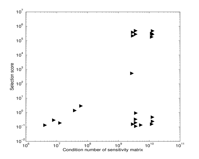
Figure 1: Parameter selection score $\displaystyle\alpha(\theta)$ versus the condition number $\displaystyle\kappa(\chi(\theta))$ of the $\displaystyle n\times p$ sensitivity matrix, for all parameter vectors $\displaystyle\theta\in\Theta_{p}$ with $\displaystyle p=5$. Logarithmic scales are used on both axes.

The subset selection algorithm was applied for $\displaystyle p=4,\dots,10$, while using the nominal variance and parameter values. We find that there is not a single parameter combination with $\displaystyle p=10$ that has a full rank sensitivity matrix. For $\displaystyle p=9$, only three parameter vectors pass the full rank test, and none of which can be considered feasible. We summarize the feasible parameter vectors in Table 1 for $\displaystyle p=4,\dots,8$, where each feasible $\displaystyle\theta\in\Theta_{p}$ is displayed along with $\displaystyle\kappa(\chi(\theta))$ and $\displaystyle\alpha(\theta)$. The cutoffs used to select the parameter combinations in Table 1 were somewhat arbitrary but relative to the smallest values computed for the two criteria (condition number and selection score) in each example.

Table 1: Feasible parameter vectors obtained while applying the subset selection algorithm for $\displaystyle p=4,\dots,8$, using nominal values as listed earlier in the text. For each selected parameter vector $\displaystyle\theta\in\Theta_{p}$ the condition number of the sensitivity matrix $\displaystyle\kappa(\chi(\theta))$, and the selection score $\displaystyle\alpha(\theta)$ are displayed.

Parameter vector $\displaystyle\theta$	Condition number $\displaystyle\kappa(\chi(\theta))$	Selection score $\displaystyle\alpha(\theta)$
$\displaystyle(L,\beta_{0},a_{1},b_{1})$	2.047$\displaystyle\times 10^{5}$	5.019$\displaystyle\times 10^{-2}$
$\displaystyle(M,\beta_{0},a_{1},b_{1})$	1.420$\displaystyle\times 10^{5}$	6.386$\displaystyle\times 10^{-2}$
$\displaystyle(P,\beta_{0},a_{1},b_{1})$	3.176$\displaystyle\times 10^{5}$	7.044$\displaystyle\times 10^{-2}$
$\displaystyle(L,D,\beta_{0},a_{1},b_{1})$	4.034$\displaystyle\times 10^{6}$	1.332$\displaystyle\times 10^{-1}$
$\displaystyle(D,M,\beta_{0},a_{1},b_{1})$	1.233$\displaystyle\times 10^{7}$	1.897$\displaystyle\times 10^{-1}$
$\displaystyle(D,P,\beta_{0},a_{1},b_{1})$	7.781$\displaystyle\times 10^{6}$	2.987$\displaystyle\times 10^{-1}$
$\displaystyle(N,L,D,\beta_{0},a_{1},b_{1})$	1.829$\displaystyle\times 10^{10}$	1.670$\displaystyle\times 10^{-1}$
$\displaystyle(S_{0},N,D,\beta_{0},a_{1},b_{1})$	1.454$\displaystyle\times 10^{10}$	2.026$\displaystyle\times 10^{-1}$
$\displaystyle(S_{0},L,D,\beta_{0},a_{1},b_{1})$	1.828$\displaystyle\times 10^{10}$	2.375$\displaystyle\times 10^{-1}$
$\displaystyle(S_{0},D,M,\beta_{0},a_{1},b_{1})$	2.152$\displaystyle\times 10^{10}$	3.301$\displaystyle\times 10^{-1}$
$\displaystyle(S_{0},D,P,\beta_{0},a_{1},b_{1})$	1.828$\displaystyle\times 10^{10}$	4.832$\displaystyle\times 10^{-1}$
$\displaystyle(N,D,M,\beta_{0},a_{1},b_{1})$	2.166$\displaystyle\times 10^{10}$	5.739$\displaystyle\times 10^{-1}$
$\displaystyle(N,D,P,\beta_{0},a_{1},b_{1})$	1.829$\displaystyle\times 10^{10}$	9.658$\displaystyle\times 10^{-1}$
$\displaystyle(N,L,D,M,\beta_{0},a_{1},b_{1})$	2.166$\displaystyle\times 10^{10}$	5.960$\displaystyle\times 10^{0}$
$\displaystyle(S_{0},L,D,M,\beta_{0},a_{1},b_{1})$	2.167$\displaystyle\times 10^{10}$	5.970$\displaystyle\times 10^{0}$
$\displaystyle(N,D,M,P,\beta_{0},a_{1},b_{1})$	2.166$\displaystyle\times 10^{10}$	1.153$\displaystyle\times 10^{1}$
$\displaystyle(S_{0},D,M,P,\beta_{0},a_{1},b_{1})$	2.167$\displaystyle\times 10^{10}$	1.159$\displaystyle\times 10^{1}$
$\displaystyle(S_{0},N,L,D,M,\beta_{0},a_{1},b_{1})$	6.333$\displaystyle\times 10^{12}$	5.044$\displaystyle\times 10^{1}$
$\displaystyle(S_{0},N,D,M,P,\beta_{0},a_{1},b_{1})$	6.561$\displaystyle\times 10^{12}$	2.950$\displaystyle\times 10^{2}$

5 Applications of the subset selection algorithm to synthetic and observed data sets

The subset selection algorithm is illustrated first by solving inverse problems from synthetic observations. To construct a synthetic data set we suppose a nominal parameter vector and a nominal error variance are equal to $\displaystyle\theta_{0}$ (true parameter vector) and $\displaystyle\sigma_{0}^{2}$ (true variance), respectively. Random noise is then added to the model output as follows:

$$Y_{j}=z(t_{j};\theta_{0})+\sigma_{0}V_{j},$$ (55)

where $\displaystyle V_{j}$ is a standard normal random variable, i.e., $\displaystyle V_{j}\sim\mathcal{N}(0,1)$. A realization $\displaystyle y_{j}$ of the observation process $\displaystyle Y_{j}$, is calculated by drawing independent samples $\displaystyle v_{j}$ from the standard normal distribution so that

$$\begin{array}[]{lr}y_{j}=z(t_{j};\theta_{0})+\sigma_{0}v_{j}&\mbox{for $\displaystyle j=1,\dots,n$}.\end{array}$$

The OLS inverse problems were solved by implementing a subspace trust region method (based on an interior-reflective Newton method [33]). We used the MATLAB (The Mathworks, Inc.) routine lsqnonlin. For the purposes of this demonstration we initialized every optimization routine at the nominal parameter vector $\displaystyle\theta_{0}$.

The nominal error variance and nominal parameter values are those given in the previous section. The parameter vectors estimated from synthetic data are those appearing on top of each subtable in Table 2, for each value of $\displaystyle p$, where parameter combinations are sorted in ascending order of their selection score (from top to bottom). In other words, all the parameter vectors estimated from synthetic observations have reasonable condition numbers and relatively small selection scores. Five inverse problems (for $\displaystyle p=8,7,6,5,4$) were solved from the same realization of the observation process, to estimate the parameter vectors

$$\begin{array}[]{c}\theta=(S_{0},N,L,D,M,\beta_{0},a_{1},b_{1}),\\ \theta=(N,L,D,M,\beta_{0},a_{1},b_{1}),\\ \theta=(N,L,D,\beta_{0},a_{1},b_{1}),\\ \theta=(L,D,\beta_{0},a_{1},b_{1}),\\ \theta=(L,\beta_{0},a_{1},b_{1}).\end{array}$$

Results of these numerical experiments are summarized in Table 2.

Table 2: Results of solving five inverse problems from a single synthetic data set generated as described in the text using nominal values listed earlier. For each parameter combination we display the estimate (Est.), the standard error (S.E.) and the coefficient of variation (standard error divided by the estimate, C.V. = S.E./Est.). For notational convenience we use here the notation $\displaystyle e$ to denote exponentiation to the base 10; i.e., $\displaystyle 2.8e^{5}$ denotes $\displaystyle 2.8\times 10^{5}$, etc.

Parameter vector $\displaystyle\theta=(S_{0},N,L,D,M,\beta_{0},a_{1},b_{1})$
	$\displaystyle S_{0}$	$\displaystyle N$	$\displaystyle L$	$\displaystyle D$	$\displaystyle M$	$\displaystyle\beta_{0}$	$\displaystyle a_{1}$	$\displaystyle b_{1}$
Est.	2.8$\displaystyle e^{5}$	1.0$\displaystyle e^{6}$	5.0$\displaystyle e^{0}$	9.6$\displaystyle e^{-3}$	5.5$\displaystyle e^{-3}$	3.7$\displaystyle e^{2}$	2.0$\displaystyle e^{-2}$	-2.0$\displaystyle e^{-2}$
S.E.	1.5$\displaystyle e^{6}$	5.0$\displaystyle e^{6}$	4.5$\displaystyle e^{1}$	3.1$\displaystyle e^{-3}$	6.2$\displaystyle e^{-2}$	3.4$\displaystyle e^{3}$	7.7$\displaystyle e^{-2}$	8.4$\displaystyle e^{-2}$
C.V.	5.5$\displaystyle e^{0}$	5.0$\displaystyle e^{0}$	9.1$\displaystyle e^{0}$	3.2$\displaystyle e^{-1}$	1.1$\displaystyle e^{1}$	9.0$\displaystyle e^{0}$	3.8$\displaystyle e^{0}$	-4.2$\displaystyle e^{0}$
Parameter vector $\displaystyle\theta=(N,L,D,M,\beta_{0},a_{1},b_{1})$
Est.		1.0$\displaystyle e^{6}$	5.0$\displaystyle e^{0}$	9.6$\displaystyle e^{-3}$	5.5$\displaystyle e^{-3}$	3.7$\displaystyle e^{2}$	2.0$\displaystyle e^{-2}$	-2.0$\displaystyle e^{-2}$
S.E.		2.7$\displaystyle e^{4}$	2.7$\displaystyle e^{0}$	2.5$\displaystyle e^{-3}$	2.2$\displaystyle e^{-2}$	5.9$\displaystyle e^{2}$	3.1$\displaystyle e^{-2}$	2.5$\displaystyle e^{-2}$
C.V.		2.7$\displaystyle e^{-2}$	5.4$\displaystyle e^{-1}$	2.6$\displaystyle e^{-1}$	4.1$\displaystyle e^{0}$	1.6$\displaystyle e^{0}$	1.6$\displaystyle e^{0}$	-1.3$\displaystyle e^{0}$
Parameter vector $\displaystyle\theta=(N,L,D,\beta_{0},a_{1},b_{1})$
Est.		1.0$\displaystyle e^{6}$	5.0$\displaystyle e^{0}$	9.6$\displaystyle e^{-3}$		3.8$\displaystyle e^{2}$	2.0$\displaystyle e^{-2}$	-2.0$\displaystyle e^{-2}$
S.E.		2.7$\displaystyle e^{4}$	1.7$\displaystyle e^{-1}$	5.8$\displaystyle e^{-4}$		1.5$\displaystyle e^{1}$	1.3$\displaystyle e^{-3}$	1.2$\displaystyle e^{-3}$
C.V.		2.7$\displaystyle e^{-2}$	3.4$\displaystyle e^{-2}$	6.1$\displaystyle e^{-2}$		3.9$\displaystyle e^{-2}$	6.3$\displaystyle e^{-2}$	-6.1$\displaystyle e^{-2}$
Parameter vector $\displaystyle\theta=(L,D,\beta_{0},a_{1},b_{1})$
Est.			5.0$\displaystyle e^{0}$	9.6$\displaystyle e^{-3}$		3.8$\displaystyle e^{2}$	2.0$\displaystyle e^{-2}$	-2.0$\displaystyle e^{-2}$
S.E.			7.4$\displaystyle e^{-2}$	5.8$\displaystyle e^{-4}$		9.8$\displaystyle e^{0}$	1.2$\displaystyle e^{-3}$	1.2$\displaystyle e^{-3}$
C.V.			1.5$\displaystyle e^{-2}$	6.1$\displaystyle e^{-2}$		2.6$\displaystyle e^{-2}$	6.2$\displaystyle e^{-2}$	-6.0$\displaystyle e^{-2}$
Parameter vector $\displaystyle\theta=(L,\beta_{0},a_{1},b_{1})$
Est.			5.0$\displaystyle e^{0}$			3.8$\displaystyle e^{2}$	2.0$\displaystyle e^{-2}$	-2.0$\displaystyle e^{-2}$
S.E.			1.4$\displaystyle e^{-2}$			2.6$\displaystyle e^{0}$	2.0$\displaystyle e^{-4}$	7.9$\displaystyle e^{-4}$
C.V.			2.7$\displaystyle e^{-3}$			6.8$\displaystyle e^{-3}$	9.9$\displaystyle e^{-3}$	-4.0$\displaystyle e^{-2}$

We analyze the results using the coefficient of variation: standard error (SE) divided by estimate (Est). For instance in Table 2, when $\displaystyle\theta=(S_{0},N,L,D,M,\beta_{0},a_{1},b_{1})$ it is seen for $\displaystyle D$ that the standard error is nearly one third of the estimate, suggesting lower uncertainty. For the other parameters $\displaystyle S_{0}$, $\displaystyle N$, $\displaystyle L$, $\displaystyle M$, $\displaystyle\beta_{0}$, $\displaystyle a_{1}$, and $\displaystyle b_{1}$ the standard error can be nearly four times (and up to eleven times) the estimate (for $\displaystyle b_{1}$ its SE is $\displaystyle|4\times\mbox{Est}|$, because $\displaystyle b_{1}<0$). This feature denotes substantial uncertainty. Figure 2(a) displays the residual plot (see [4] for a discussion of the effective use of residual plots) for this parameter combination: $\displaystyle y_{j}-z(t_{j};\hat{\theta}_{OLS})$ versus time $\displaystyle t_{j}$, where $\displaystyle j=1,\dots,n$. The temporal pattern in the residuals together with large standard errors suggest that estimation of this parameter combination from observations (with a statistical error structure) would be meaningless.

The residual plots for all the other parameter combinations in Table 2 do not have temporal patterns. For the sake of illustration we display in Figure 2(b) the residuals versus time for $\displaystyle\theta=(L,D,\beta_{0},a_{1},b_{1})$.

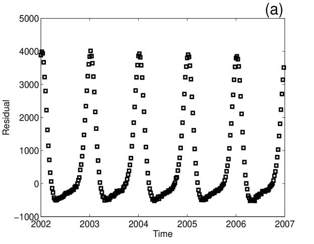
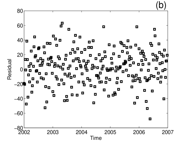
Figure 2: Residual plots: $\displaystyle y_{j}-z(t_{j};\hat{\theta}_{OLS})$, versus time, $\displaystyle t_{j}$, for $\displaystyle j=1,\dots,n$. Graph (a) displays residuals obtained for $\displaystyle\theta=(S_{0},N,L,D,M,\beta_{0},a_{1},b_{1})$, while Graph (b) depicts residuals for $\displaystyle\theta=(L,D,\beta_{0},a_{1},b_{1})$.

Improvements in uncertainty quantification are observed with the removal of some key parameters. We think it is not just reducing the number $\displaystyle p$ of parameters, but rather which parameters are to be estimated that really counts. The near dependence in the columns of the sensitivity matrix $\displaystyle\chi$ reflects correlations between parameter estimates which make a parameter combination unsuitable for estimation. For instance, consider the removal of $\displaystyle S_{0}$ from the estimation, and compare $\displaystyle\theta=(S_{0},N,L,D,M,\beta_{0},a_{1},b_{1})$ with $\displaystyle\theta=(N,L,D,M,\beta_{0},a_{1},b_{1})$ in Table 2. The standard error for $\displaystyle N$ is seen to drop from 500% to approximately 3% of the estimate. Another substantial improvement when dropping $\displaystyle S_{0}$ is obtained for $\displaystyle L$, for which its standard error reduces from being nine times the estimate to one half of its value. Lower uncertainty improvements are also obtained for the parameters $\displaystyle M$, $\displaystyle\beta_{0}$, $\displaystyle a_{1}$, and $\displaystyle b_{1}$.

The next numerical experiment considered here is the removal of $\displaystyle S_{0}$ and $\displaystyle M$. We compare the results for $\displaystyle\theta=(S_{0},N,L,D,M,\beta_{0},a_{1},b_{1})$ with those for $\displaystyle\theta=(N,L,D,\beta_{0},a_{1},b_{1})$, in Table 2. There are uncertainty improvements for all parameters. The least (but still substantial) improvement is for $\displaystyle D$, where its standard error drops from being nearly 30% to being just 6% of the estimate. For the parameters $\displaystyle N$, $\displaystyle L$, $\displaystyle\beta_{0}$, $\displaystyle a_{1}$, and $\displaystyle b_{1}$ an improvement of two orders of magnitude is seen. Improvements in uncertainty are more pronounced after removing $\displaystyle S_{0}$, $\displaystyle N$, and $\displaystyle M$: for this we compare $\displaystyle\theta=(S_{0},N,L,D,M,\beta_{0},a_{1},b_{1})$ and $\displaystyle\theta=(L,D,\beta_{0},a_{1},b_{1})$ in Table 2.

Undoubtedly, the best case scenario of uncertainty quantification we obtained is that of estimating $\displaystyle\theta=(L,\beta_{0},a_{1},b_{1})$ from the same synthetic data set. In Table 2, it is seen that the standard errors reduce to less than 1% of the estimates for $\displaystyle L$, $\displaystyle\beta_{0}$, and $\displaystyle a_{1}$, and to 4% from nearly 400% of the estimate for $\displaystyle b_{1}$.

As a final note in this section, we present results obtained from solving the OLS problem while using observations of an influenza-like-illness in France [38]. Some of the parameters were fixed to values suggested in [15, 16, 20]:

$$\begin{array}[]{l}S_{0}=1.56\times 10^{7}\mbox{(people)},\ E_{0}=6.44\mbox{(people)},\ I_{0}=12.88\mbox{(people)},\ N=6.40\times 10^{7}\mbox{(people)},\\ L=6.00\mbox{(years)},\ D=1.10\times 10^{-2}\mbox{(years)},\ M=5.50\times 10^{-3}\mbox{(years)},\ P=80.87\mbox{(years)}.\end{array}$$

The inverse problem was solved with $\displaystyle\theta=(\beta_{0},a_{1},b_{1})$. Simple inspection of the standard errors in Table 3 does not seem to immediately suggest there is a poor fit (not displayed here). Roughly speaking, the standard error is: 13% of the estimate for $\displaystyle\beta_{0}$; 30% of the estimate for $\displaystyle a_{1}$; 45% of the estimate for $\displaystyle b_{1}$. These calculations give an indication of wide uncertainty, but they are not as extreme as the results for $\displaystyle\theta=(S_{0},N,L,D,M,\beta_{0},a_{1},b_{1})$ in Table 2. One can easily be misled by invalid uncertainty quantification in the absence of residual analysis. Residual plots (not displayed here) in this case have systematic patterns, suggesting that either the statistical model (equation (15)) may be incorrect, or more likely, the SEIRS model fails to adequately describe the underlying process.

Table 3: Estimates from influenza-like-illness observations, where $\displaystyle\theta=(\beta_{0},a_{1},b_{1})$. The coefficient of variation is defined as the standard error divided by the estimate.

Parameter	Estimate	Standard error	Unit	Coefficient of variation
$\displaystyle\beta_{0}$	3.100$\displaystyle\times 10^{2}$	4.055$\displaystyle\times 10^{1}$	years-1	1.308$\displaystyle\times 10^{-1}$
$\displaystyle a_{1}$	1.539$\displaystyle\times 10^{-2}$	4.588$\displaystyle\times 10^{-3}$	1	2.981$\displaystyle\times 10^{-1}$
$\displaystyle b_{1}$	-2.406$\displaystyle\times 10^{-2}$	1.090$\displaystyle\times 10^{-2}$	1	-4.530$\displaystyle\times 10^{-1}$

6 Discussion

We have discussed a computational methodology for inverse problem formulation in the context of parameter identifiability. Using an OLS scheme based on a constant variance statistical model for the observation process and a seasonal SEIRS epidemics model for illustration, we have proposed a prior-analysis algorithm that we believe might profitably precede efforts on parameter estimation from data. The algorithm can be used if reasonable ranges for the sought after parameters are either known a priori, or can be assumed by the user much in the same way one must assume reasonable ranges in inverse problem formulations and initiation of algorithms for the resulting estimation procedures.

The subset selection [31] algorithm given in Section 4 is based on two main criteria for a fixed number of parameters: (i) full rank of the sensitivity matrix; and (ii) calculation of standard errors. We proposed to first select according to the sensitivity matrix rank, because those parameter combinations for which $\displaystyle\chi$ has full rank will have a non-singular Fisher information matrix $\displaystyle\chi^{T}\chi$, and its inverse is used in the calculation of the standard errors (see equation (26)).

The near dependence of the sensitivity matrix columns can be a fingerprint of parameter correlations–a pertinent feature for subset selection [31]. Capaldi, et al., [14] determine identifiability of parameters in a simple SIR model, and show how correlation between parameter estimates can impede the estimation of other parameters and parameter combinations, such as the basic reproductive number. Moreover, Brun, et al., [11] explain that if the columns of $\displaystyle\chi$ are nearly dependent, then changes in the model output due to small changes in a single parameter can be compensated by appropriate changes in other parameters.

We have presented illustrations of the how the removal of nearly dependent columns of the sensitivity matrix can provide substantial improvements in uncertainty quantification. This feature involves more than just reducing the number $\displaystyle p$ of parameters, it relates to excluding certain key parameters. For instance, if we assume a linear Taylor expansion of the model output, the estimator $\displaystyle\theta_{OLS}\in\mathbb{R}^{p}$ is given by equation (44), where the sensitivity matrix $\displaystyle\chi(\theta_{0})$ has singular values $\displaystyle s_{1}\geq\dots\geq s_{p-1}\geq s_{p}>0$. If $\displaystyle s_{p}\approx 0$ and $\displaystyle s_{p-1}>1$, then submatrices with singular values $\displaystyle s_{2}\geq\dots\geq s_{p}>0$, and $\displaystyle s_{1}\geq\dots\geq s_{p-1}$, have different conditioning when quantifying the sensitivity of reduced order estimations that only involve $\displaystyle p-1$ parameters. The condition number of the former submatrix is $\displaystyle s_{2}/s_{p}$, which is large if $\displaystyle s_{p}\approx 0$, while for the latter submatrix the condition number satisfies $\displaystyle 1\leq s_{1}/s_{p-1}<s_{1}$, because $\displaystyle s_{p-1}>1$.

In our numerical experiments, we calculate sensitivity matrices $\displaystyle\chi(\theta)$ evaluated at different realizations of the estimator $\displaystyle\theta=\hat{\theta}_{OLS}$. When $\displaystyle\theta=(S_{0},N,L,D,M,\beta_{0},a_{1},b_{1})$ the singular values of the sensitivity matrix range from $\displaystyle 4.7\times 10^{6}$ to $\displaystyle 4.6\times 10^{-6}$ while for $\displaystyle\theta=(L,\beta_{0},a_{1},b_{1})$ the singular values of $\displaystyle\chi(\hat{\theta}_{OLS})$ range from $\displaystyle 1.9\times 10^{6}$ to $\displaystyle 9.3\times 10^{0}$.

The smallest singular value changes from $\displaystyle 4.6\times 10^{-6}$ to $\displaystyle 9.3\times 10^{0}$ while the largest remain on the order of $\displaystyle 10^{6}$. This improvement in conditioning is reflected in the the standard error for $\displaystyle L$, $\displaystyle\beta_{0}$, and $\displaystyle a_{1}$, which reduces to less than 1% of the estimate, from nearly 900% and 380% (see Table 2).

Although in this paper we only discuss OLS, the selection algorithm can be easily applied when using a generalized least squares scheme [4]. We also carried out numerical experiments (for brevity not discussed here) involving use of synthetic nonconstant variance data sets in GLS formulations, and obtained results absolutely consistent with those of the OLS formulation presented here (Section 5).

References

- [1] R. Anderson and B.T. Grenfell, Oscillatory fluctuations in the incidence of infectious disease and the impact of vaccination: time series analysis, J. Hyg. Camb., 93 (1984), 587–608.
- [2] D.T. Anh, M.P. Bonnet, G. Vachaud, C.V. Minh, N. Prieur, L.V. Duc and L.L. Anh, Biochemical modeling of the Nhue River (Hanoi, Vitenam): practical identifiability analysis and parameter estimation, Ecol. Model., 193 (2006), 182–204.
- [3] K.J. Astrom and P. Eykhoff, System identification–A survey, Automatica, 7 (1971), 123–162.
- [4] H.T. Banks, M. Davidian, J.R. Samuels and K.L. Sutton, An inverse problem statistical methodology summary, Center for Research in Scientific Computation Technical Report CRSC-TR08-1, NCSU, January, 2008; in Mathematical and Statistical Estimation Approaches in Epidemiology, (eds. G. Chowell, et. al.), Springer, New York, 2009, pp. 249–302.
- [5] H.T. Banks, S. Dediu and S.E. Ernstberger, Sensitivity functions and their uses in inverse problems, CRSC Tech Report, CRSC-TR07-12, NCSU, July, 2007; J. Inverse and Ill-posed Problems, 15 (2007), 683–708.
- [6] H.T. Banks, S. Dediu, S.L. Ernstberger, F. Kappel, A new approach to optimal design problems, Center for Research in Scientific Computation Technical Report CRSC-TR08-12, NCSU, September, 2008.
- [7] H. T. Banks, S. L. Ernstberger and S. L.Grove, Standard errors and confidence intervals in inverse problems: sensitivity and associated pitfalls, J. Inverse and Ill-posed Problems, 15 (2007), 1–18.
- [8] H.T. Banks and J.R. Samuels, Jr., Detection of cardiac occlusions using viscoelastic wave propagation, CRSC-TR08-23, December, 2008; Advances in Applied Mathematics and Mechanics, 1 (2009), 1–28.
- [9] R. Bellman and K.M. Astrom, On structural identifiability, Math. Biosci., 7 (1970), 329–339.
- [10] R. Bellman and R. Kalaba, Quasilinearization and Nonlinear Boundry Value Problems, American Elsevier, New York, 1965.
- [11] R.Brun, M. Kuhni, H. Siegrist, W. Gujer and P. Reichert, Practical identifiability of ASM2d parameters — systematic selection and tuning of parameter subsets, Water Res., 36 (2002), 4113–4127.
- [12] K.P. Burnham and D.R. Anderson, Model Selection and Multimodel Inference: A Practical Information-Theoretic Approach, Springer-Verlag, New York, 2002.
- [13] M. Burth, G.C. Verghese and M. Vélez-Reyes, Subset selection for improved parameter estimation in on-line identification of a synchronous generator, IEEE T. Power Syst., 14 (1999), 218–225.
- [14] A. Capaldi, S. Behrend, B. Berman, J. Smith, J. Wright and A.L. Lloyd, Parameter estimation and uncertainty quantification for an epidemic model, in preparation.
-
[15]
Central Intelligence Agency World Factbook (2008),
https://www.cia.gov/library/publications/the-world-factbook/index.html, cited 12 Nov 2008. - [16] G. Chowell, M.A. Miller and C. Viboud, Seasonal influenza in the United States, France, and Australia: transmission and prospects for control, Epidemiol. Infect., 136 (2008), 852–864.
- [17] A. Cintrón-Arias, C. Castillo-Chávez, L.M.A. Bettencourt, A.L. Lloyd, and H.T. Banks, The estimation of the effective reproductive number from disease outbreak data, Center for Research in Scienti c Computation Technical Report CRSC-TR08-08, NCSU, April, 2008; Math. Biosci. Engr., 6 (2009), 261–283.
- [18] C. Cobelli and J. J. DiStefano III, Parameter and structural identifiability concepts and ambiguities: a critical review and analysis, Am. J. Physiol. 239 (1980), R7–R24.
- [19] M. Davidian and D.M. Giltinan, Nonlinear Models for Repeated Measurement Data, Chapman & Hall, Boca Raton, 1995.
- [20] J. Dushoff, J.B. Plotkin, S.A. Levin and D.J. Earn, Dynamical resonance can account for seasonality of influenza epidemics, P. Natl. Acad. Sci. USA, 101 (2004), 16915–16916.
- [21] N.D. Evans, L.J. White, M.J. Chapman, K.R. Godfrey and M.J. Chappell, The structural identifiability of the susceptible infected recovered model with seasonal forcing, Math. Biosci., 194 (2005), 175–197.
- [22] P. Eykhoff, System Identification: Parameter and State Estimation, Wiley & Sons, New York, 1974.
- [23] K. Glover and J.C. Willems, Parametrizations of linear dynamical systems: Canonical forms and identifiability, IEEE Trans. Automat. Contr., AC-19 (1974), 640–645.
- [24] G.H. Golub and C.F. Van Loan, Matrix Computations, Johns Hopkins University Press, Baltimore, 1996.
- [25] N.C. Grassly and C. Fraser, Seasonal infectious disease epidemiology, P. Roy. Soc. B-Biol. Sci., 273 (2006), 2541–2550.
- [26] A. Holmberg, On the practical identifiability of microbial growth models incorporating Michaelis-Menten type nonlinearities, Math. Biosci., 62 (1982), 23–43.
- [27] M. Kalivianakis, S.L.J. Mous and J. Grasman, Reconstruction of the seasonally varying contact rate for measles, Math. Biosci., 124 (1994), 225–234.
- [28] R.E Kalman, Mathematical description of linear dynamical systems, SIAM J. Control, 1 (1963), 152–192.
- [29] Y.A. Kuznetsov and C. Piccardi, Bifurcation analysis of epidemic SEIR and SIR epidemic models, J. Math. Biol., 32 (1994), 109–121.
- [30] A.K. Mehra and D.G. Lainiotis, System Identification, Academic Press, New York, 1976.
- [31] A.J. Miller, Subset Selection in Regression, Chapman & Hall, New York, 1990.
- [32] I.M. Navon, Practical and theoretical aspects of adjoint parameter estimation and idenrtifiability in meteorology and oceanography, Dyn. Atmospheres and Oceans, 27 (1997), 55–79.
- [33] J. Nocedal and S.J. Wright, Numerical Optimization, Springer-Verlag, New York, 1999.
- [34] J.G. Reid, Structural identifiability in linear time-invariant systems, IEEE Trans. Automat. Control, 22 (1977), 242–246.
- [35] F. Riedo, B. Plikaytis and C. Broome, Epidemiology and prevention of meningococcal disease, Pediatr. Infect. Dis. J., 14 (1995), 643–657.
- [36] A.P. Sage and J.L. Melsa, System Identification, Academic Press, New York, 1971.
- [37] G.A.F. Seber and C.J. Wild, Nonlinear Regression, John Wiley & Sons, Chichester, 2003.
-
[38]
Sentinelles Influenza-like Illness (2008),
http://websenti.b3e.jussieu.fr/sentiweb/?page=maladies&mal=3, cited 12 Nov 2008. - [39] I.B. Schwartz and H.L. Smith, Infinite subharmonic bifurcation in an SEIR epidemic model, J. Math. Biol., 18 (1983), 233–253.
- [40] K. Thomaseth and C. Cobelli, Generalized sensitivity functions in physiological system identification, Annals of Biomedical Engineering, 27 (1999), 607–616.
- [41] L.J. White, N.D. Evans, T.J.G.M. Lam, Y.H. Schukken, G.F. Medley, K.R. Godfrey and M.J. Chappell, The structural identifiability and parameter estimation of a multispecies model for the transmission of mastitis in diary cows, Math. Biosci., 174 (2001), 77–90.
- [42] J. Witte, A. Karchmer, M. Case, K.L. Hermann, E. Abrutyn, I. Kassanof, et al.:, Epidemiology of rubella, Am. J. Dis. Child., 118 (1969), 107–111.
- [43] H. Wu, H. Zhu, H. Miao and A.S. Perelson, Parameter identifiability and estimation of HIV/AIDS dynamics models, Bull. Math. Biol., 70 (2008), 785–799.
- [44] X. Xia and C.M. Moog, Identifiability of nonlinear systems with application to HIV/AIDS models, IEEE T. Automat. Contr., 48 (2003), 330–336.
- [45] H. Yue, M. Brown, F. He, J. Jia and D.B. Kell, Sensitivity analysis and robust experimental design of a signal transduction pathway system, Int. J. Chem. Kinet., 40 (2008), 730–741.