On the complex behaviour of the density in composite quantum systems.

Abstract

In this paper, we study how the probability of presence of a particle is distributed between the two parts of a composite fermionic system. We uncover that the difference of probability depends on the energy in a striking way and show the pattern of this distribution. We discuss the main features of the latter and explain analytically those that we understand. In particular, we prove that it is a non-perturbative property and we find out a large/small coupling constant duality. We also find and study features that may connect our problem with certain aspects of non linear classical dynamics, like the existence of resonances and sensitive dependence on the state of the system. We show that the latter has indeed a similar origin than in classical mechanics: the appearance of small denominators in the perturbative series. Inspired by the proof of KAM theorem, we are able to deal with this problem by introducing a cut-off in energies that eliminates these small denominators. We also formulate some conjectures that we are not able to prove at present but can be supported by numerical experiments.

I Introduction

In spite of its apparent simplicity, many-body quantum systems in one dimension have turned out to be very useful models in order to understand and unravel many different phenomena, from entanglement Latorre ; Jin ; Ares1 ; Ares2 ; Ares3 ; Ares8 and quantum information Amico ; Laflorencie to new phases of matter Asboth ; Bernevig ; Viyuela ; Viyuela2 and quantum chaos Alessio . Moreover, the development of experimental techniques in cold atoms, ion traps and polarized molecules has recently allowed to simulate these systems in the laboratory Bloch ; Porras ; Blatt ; Atala ; Micheli ; Yan ; Kuznetsova .

Two of the most studied unidimensional many-body quantum systems are the tight binding model and the Su-Schrieffer-Heeger (SSH) model. The tight binding model consists of a lattice with a fixed number of free fermions which can hop from one site to the next one with a given probability. In the simplest version of the model, the sites of the lattice (the position of the atoms) are fixed and the hopping probability (the hopping integral) is constant along the chain. Physically, this system can be seen as a toy model for a one-dimensional metal. It can also be mapped into the XX spin chain via the Jordan-Wigner transformation. When the atom vibrations are taken into account, the hopping probability depends on the position of the nearest sites and, due to the Peierls theorem, the chain dimerizes. In the Born-Oppenheimer approximation the hopping probabilities between the even-odd and odd-even sites are different. This is the SSH model, which describes a unidimensional insulator. It was firstly introduced to characterize solitons in the polyacetylene molecule ssh ; ssh2 ; Casahorran . In last years, the SSH model has attracted much attention since it displays the essential properties of topological insulators Asboth ; Bernevig .

In this paper, we take the union of two different systems of this type. That is, we analyze systems composed by two different tight binding models coupled by special bonds which we will call contacts. Physically, this situation corresponds to the junction of two metals with different band structure. We may also combine a tight binding model and a SSH model (metal-insulator) or two SSH models (insulator-insulator). These kinds of junctions were considered in Ref. Eisler , in which the ground state entanglement entropy between the two parts is investigated; see also Peschel ; Sakai . Systems with two different critical parts (such as the tight binding model) or with a critical and a non-critical part (like the SSH model) have been examined from the perspective of conformal invariance Hinrichsen ; Berche ; Zhang1 ; Zhang2 . Composite free-fermionic systems are also of interest in quantum transport and non equilibrium physics Antal ; Barnabe ; Biella ; Calabrese ; Eisler2 ; Stephan ; Kennes ; Viti ; Allegra ; Dubail ; Biella2 ; Prosen ; Gawedzki ; Gawedzki2 ; Moosavi , where a typical problem is the analysis of the evolution of the overall state of two different chains after being joined together (inhomogeneous quench).

Here, we consider the one particle states with a definite energy. Depending on its energy, the particle is confined in one of the two parts or, on the contrary, is delocalized along the whole chain. In this work, we will analyze how the particle distributes between the two parts. In a way, our problem is not how, but where Schrödinger’s cat is. For this purpose, we will introduce a quantity that we call leaning, defined as the difference between the probabilities of finding the particle in each part of the chain. It happens that the dependence of the leaning on the energy and on the contact between the two parts is rather non-trivial Uson . The goal of this paper is to characterize and explain this behaviour.

The paper is organized as follows. In Section II, we introduce the main system under study, the union of two tight binding models, and the so-called leaning. In Section III, we will see how to compute analytically the leaning of a one-particle configuration. In Section IV, we calculate the spectral density of the whole chain. Sections V and VI are devoted respectively to analyze the resonant regions and to determine the boundary of the clouds of points that appear in the energy-leaning plot. In Section VII, we conjecture the existence of a measure in the energy-leaning plane that accounts for the density of points in the thermodynamic limit. Finally, in Section VIII, we present our conclusions and outlook. The paper is complemented with an Appendix where we show that the average of the leaning does not depend on the value of the contact.

II Basic set-up

As we already mentioned in the introduction, the system that we are going to study consists of the union of two tight binding fermionic chains of lengths $N_{1}$ and $N_{2}$ with hopping parameters $t_{1}$ and $t_{2}$ respectively. The ends of the two chains are connected by means of other hoppings $t_{0},t_{0}^{\prime}$ which we call contacts, these will be our main tunable parameters.

Therefore, the Hamiltonian of the composite system is

$$H=\frac{1}{2}\left(t_{1}\sum_{n=1}^{N_{1}-1}(a_{n}^{\dagger}a_{n+1}+a_{n+1}^{\dagger}a_{n})+t_{2}\sum_{m=1}^{N_{2}-1}(b_{m}^{\dagger}b_{m+1}+b_{m+1}^{\dagger}b_{m})\hskip 14.22636pt\right.$$ (1)

$$\left.+t_{0}(a_{N_{1}}^{\dagger}b_{N_{2}}+b_{N_{2}}^{\dagger}a_{N_{1}})+t^{\prime}_{0}(b_{1}^{\dagger}a_{1}+a_{1}^{\dagger}b_{1})\right),$$ (2)

where $a_{n},b_{m}$ are the fermionic annihilation operators associated to every piece of the composite chain. Note that the sites are enumerated such that the site $n=1$ of the subchain with hopping $t_{1}$ is connected with the site $m=1$ of the subchain with hopping $t_{2}$ by the contact coupling $t_{0}^{\prime}$ and, likewise, the site $n=N_{1}$ is connected with the site $m=N_{2}$ by the contact $t_{0}$ (that is, the sites of the subchain with hopping $t_{2}$ are numbered in opposite direction to those of the subchain with hopping $t_{1}$).

This kind of systems has some interesting properties that deserve further research. For instance, at certain values of the contacts it possesses a discrete spectrum with localized, topologically protected states. They behave similarly to those of the topological insulators. These features will be studied elsewhere. Here we are rather interested in the continuous spectrum (in the thermodynamic limit) and more precisely in its one particle states

$$\Psi=\left(\sum_{n=1}^{N_{1}}\alpha_{n}a^{\dagger}_{n}+\sum_{m=1}^{N_{2}}\beta_{m}b^{\dagger}_{m}\right)\mathinner{|{0}\rangle},$$ (3)

where $\mathinner{|{0}\rangle}$ represents the vacuum of the Fock space, i.e. $a_{n}\mathinner{|{0}\rangle}=b_{m}\mathinner{|{0}\rangle}=0$ $\forall m,n$.

The continuous spectrum in the composite system has a band structure that is obtained as a superposition of those corresponding to every of its two parts. In fig. 1 we represent this situation.

Figure 1: In the figure we represent the band structure of one particle states for the two separate subsystems (on the left) and the combined spectrum when we connect them (on the right). In the latter case and for particular values of the contacts $t_{0},t_{0}^{\prime}$ there could be localized states with energy in the discrete spectrum, outside the band. Here we are not interested in these states and we do not represent them.

For definiteness and without lose of generality, we shall take $t_{2}>t_{1}>0$. Then, the states whose energies are such $t_{2}>|E|>t_{1}>0$ are mainly supported in the region with hopping parameter $t_{2}$ and hardly penetrate, with exponential decay, in the left hand side. On the contrary, those states with energy in the interval $[-t_{1},t_{1}]$ are distributed along the whole chain. Our concern in this work is how the latter split between the two parts of the chain.

Therefore, we decompose the one particle Hilbert space

$${\mathcal{H}}={\mathcal{H}}_{1}\oplus{\mathcal{H}}_{2},$$

where ${\mathcal{H}}_{1}$ contains the wave functions supported in the left hand side ($\beta_{m}=0$) and ${\mathcal{H}}_{2}$ those supported in the right hand side ($\alpha_{n}=0$) and denote by $P_{1}$ and $P_{2}$ the corresponding orthogonal projectors; we shall be interested in the expectation value of the difference between these projectors

$${L}={\mathinner{\langle{\Psi}|}(P_{2}-P_{1})\mathinner{|{\Psi}\rangle}}.$$

We will refer to ${L}$ as the leaning. It measures the difference between the probability of finding the particle in the right hand side and that of finding it in the left one.

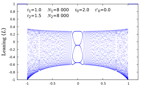
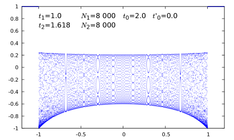
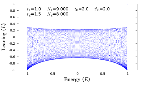
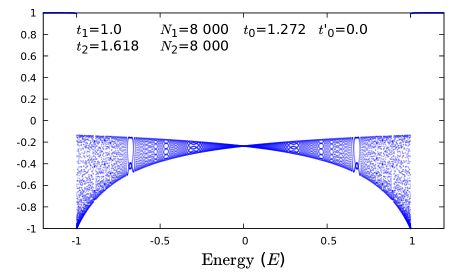
The leaning associated to a one particle stationary state $\Psi_{E}$ will be denoted by ${L}_{E}$. It is immediate to see that, in the thermodynamic limit, ${L}_{E}=1$ for $|E|\in[t_{1},t_{2}]$, however, when $E\in[-t_{1},t_{1}]$ the leaning depends on the energy in a rather complex way, as it is shown in fig. 2.

Figure 2: In these plots we show the dependence of the leaning (in the vertical axis) as a function of the energy (in horizontal axis) for different values of the hoppings $t_{1}$ and $t_{2}$, sizes $N_{1}$ and $N_{2}$ of the two subsystems, and contacts $t_{0}$, $t_{0}^{\prime}$. The two plots on the left differ in the size of one of the subsystems $N_{1}$. The two on the right in the value of the contact $t_{0}$.

The rest of the paper is devoted to understand this behaviour as fully as possible.

In first place, we see a cloud of points that fills a definite region in the $E$-${L}$ plane, apparently bounded by smooth curves. The cloud is symmetric under the exchange of $E$ to $-E$. We also observe that the points seem to be randomly distributed inside the region, except for some range of energy where they group at some definite values of ${L}$ and lie along visible curves. We call these zones resonant. We will study the origin of the previous facts and how they depend on the parameters and size of the system. Further properties of these plots will be discussed along this work.

III Analytic approach.

In this section we will show how to determine analytically the leaning of a given eigenstate.

The coefficients $\alpha_{n}$ and $\beta_{n}$ for an eigenfunction of the Hamiltonian with energy $E$, such that $|E|<t_{1}<t_{2}$, can be written as

$$\alpha_{n}=A_{1}\sin(n{k}_{1}+\delta_{1}),\quad\beta_{n}=A_{2}\sin(n{k}_{2}+\delta_{2}),$$

where

$${k}_{j}(E)=\arccos\frac{E}{t_{j}},\quad j=1,2,$$

and the following gluing conditions should be fulfilled

$$A_{1}t_{1}\sin(N_{1}{k}_{1}+{k}_{1}+\delta_{1})-A_{2}t_{0}\sin(N_{2}{k}_{2}+\delta_{2})=0,$$ (4)

$$A_{1}t_{0}\sin(N_{1}{k}_{1}+\delta_{1})-A_{2}t_{2}\sin(N_{2}{k}_{2}+{k}_{2}+\delta_{2})=0,$$ (5)

$$A_{1}t_{1}\sin(\delta_{1})-A_{2}t^{\prime}_{0}\sin({k}_{2}+\delta_{2})=0,$$ (6)

$$A_{1}t^{\prime}_{0}\sin({k}_{1}+\delta_{1})-A_{2}t_{2}\sin(\delta_{2})=0.$$ (7)

From the compatibility of these equations we derive the spectral condition and henceforth the allowed values for $E$.

In order to simplify the analysis, we shall take $t^{\prime}_{0}=0$ and, therefore, the last two equations imply $\delta_{1}=\delta_{2}=0$. We shall show along the paper that this assumption does not affect, in fact, the generality of our results.

Hence the other two equations can be equivalently written

$$C\equiv A_{2}/A_{1}=\frac{t_{1}}{t_{0}}\frac{\sin(N_{1}{k}_{1}+{k}_{1})}{\sin(N_{2}{k}_{2})}=\frac{t_{0}}{t_{2}}\frac{\sin(N_{1}{k}_{1})}{\sin(N_{2}{k}_{2}+{k}_{2})},$$ (8)

and finally

$${L}=\frac{N_{1}-N_{2}C^{2}}{N_{1}+N_{2}C^{2}}$$ (9)

is determined once the value of $E$ is fixed.

Equation (8) is our starting point for the study of plots in fig. 2. In the next sections we will focus on different aspects or characteristics of these plots and we will show how they emerge from (8). But before going to that, we shall insert a paragraph to explain the symmetry under the exchange of $E$ with $-E$ that we observe in the plots.

This is due to a chiral transformation in the states that reverses the sign of the Hamiltonian. Namely, for a one particle state (3), we define its chiral transformed state by

$$\Gamma\Psi=\left(\sum_{n=1}^{N_{1}}(-1)^{n}\alpha_{n}a^{\dagger}_{n}-\sum_{m=1}^{N_{2}}(-1)^{m}\beta_{m}b^{\dagger}_{m}\right)\mathinner{|{0}\rangle}.$$

If $N_{1}+N_{2}$ is even or $t_{0}t_{0}^{\prime}=0$, the Hamiltonian (1) satisfies $\Gamma H\Gamma=-H$ while, for the projectors $P_{1}$, $P_{2}$, we have $\Gamma P_{i}\Gamma=P_{i}$. That is, the chiral symmetry reverses the sign of the energy without changing the leaning of the state. This explains the symmetry in the plots of fig. 2.

IV Spectral density

In this section we compute the spectral density $\lambda_{t_{0}}(E)$ of the composite system in the thermodynamic limit (when the size of the chain goes to infinity) while keeping the relative size of the two chains fixed, $N_{1}=\nu_{1}N$ and $N_{2}=\nu_{2}N$. In order to make the computation simpler, we will take $t_{0}^{\prime}=0$.

Call $\Sigma_{t_{0},N}$ the spectrum of $H$ for given values of $t_{0}$ and $N$, ($t_{1},t_{2},\nu_{1},\nu_{2}$ remain fixed and, to simplify the notation, are omitted in the symbol used for the spectrum). We are interested in the region of the spectrum where the bands of the two pieces of the chain overlap, i. e. $E\in(-t_{1},t_{1})$. We define the spectral density as

$$\lambda_{t_{0}}(E)=\lim_{\delta E\to 0^{+}}\frac{1}{2\,\delta E}\lim_{N\to\infty}N^{-1}\,\sharp\!\left(\Sigma_{t_{0},N}\cap[E-\delta E,E+\delta E]\right),$$ (10)

where the symbol $\sharp$ stands for the cardinality of the set.

We will show that the density of states is actually independent of $t_{0}$ and can be computed by simply adding up the density of the two pieces. The latter can be easily estimated by going from $k$ space, where the points in the spectrum are regularly spaced by intervals $\pi/(N_{i}+1)$, to the $E$ space. As a result one gets

$$\lambda_{t_{0}}(E)=\frac{\nu_{1}k^{\prime}_{1}(E)+\nu_{2}k^{\prime}_{2}(E)}{\pi}=\frac{\nu_{1}/{\sqrt{t_{1}^{2}-E^{2}}}+\nu_{2}/{\sqrt{t_{2}^{2}-E^{2}}}}{\pi}.$$ (11)

One might be tempted to approach the problem by using perturbation theory. Actually, if we decompose the Hamiltonian in (1) as $H=H_{0}+H_{I}$ with $H_{0}$ the unperturbed piece and the perturbation given by the contact term

$$H_{I}=\frac{t_{0}}{2}(a_{N_{1}}^{\dagger}b_{N_{2}}+b_{N_{2}}^{\dagger}a_{N_{1}})+\frac{t^{\prime}_{0}}{2}(b_{1}^{\dagger}a_{1}+a_{1}^{\dagger}b_{1}),$$

one immediately sees that for $\varphi_{k},\varphi_{k^{\prime}}$ eigenstates of $H_{0}$

$$\mathinner{\langle{\varphi_{k}}|}H_{I}\mathinner{|{\varphi_{k^{\prime}}}\rangle}=O\left(\frac{1}{N}\right),$$

and, therefore, the interaction between the two pieces decreases when the system gets larger. While this is true, if we try to apply the perturbative expansion we have to face a sort of “small denominators” problem, well known in classical perturbation theory. In fact, when $N$ grows, the gaps $E^{0}_{m}-E^{0}_{m^{\prime}}$, which appear in the denominators of the perturbative expansion, can be arbitrarily small (even smaller than $O(1/N)$ for certain values of $m,m^{\prime}$) and the perturbative expansion ceases to make sense.

Another indication that we are dealing with a non perturbative phenomenon is the fact that, while for $t_{0},t_{0}^{\prime}=0$ the only two possible values for the leaning are 1 or $-1$, for any value of $t_{0}\not=0$ we have (with $N$ large enough) states with an arbitrary value for ${L}$ in the interval $[-1,1]$. This means that we can not approximate perturbatively the states of the composite system.

To avoid these potential problems we shall take a non perturbative avenue to estimate the energy eigenvalues.

We are interested in the case $t^{\prime}_{0}=0$ in which the equations (8) apply and the spectrum $\Sigma_{t_{0},N}$ is given by the solutions for $E$ of the equation

$$\frac{t_{0}^{2}}{t_{1}t_{2}}=\frac{\sin(N_{1}{k}_{1}+{k}_{1})\sin(N_{2}{k}_{2}+{k}_{2})}{\sin(N_{1}{k}_{1})\sin(N_{2}{k}_{2})}.$$ (12)

Recall that $k_{i}$ and the energy are related by $E=t_{i}\cos k_{i}$.

In the two extreme limits, $t_{0}=0$ and $t_{0}\to\infty$, it is easy to determine $\Sigma_{t_{0},N}$. Actually, for $t_{0}=0$, $\Sigma_{0,N}$ is the union of the spectra of the two parts of the composite system with Dirichlet boundary conditions, that is

$$\Sigma_{0,N}=\{E^{0}_{m};\ m=1,\dots,N_{1}+N_{2}\}=$$

$$\hskip-170.71652pt=\left\{t_{1}\cos\left(\frac{\pi m_{1}}{N_{1}+1}\right);\ m_{1}=1,\dots,N_{1}\right\}\cup\left\{t_{2}\cos\left(\frac{\pi m_{2}}{N_{2}+1}\right);\ m_{2}=1,\dots,N_{2}\right\}.$$

Similarly for $t_{0}\to\infty$ the spectrum is given by

$$\Sigma_{\infty,N}=\{E^{\infty}_{m};\ m=1,\dots,N_{1}+N_{2}-2\}=$$

$$\hskip-213.39566pt=\left\{t_{1}\cos\left(\frac{\pi m_{1}}{N_{1}}\right);\ m_{1}=1,\dots,N_{1}-1\right\}\cup\left\{t_{2}\cos\left(\frac{\pi m_{2}}{N_{2}}\right);\ m_{2}=1,\dots,N_{2}-1\right\}.$$

One may notice that in the latter case the spectrum has two points less than for $t_{0}=0$. Actually, the missing eigenvalues correspond, for large but finite $t_{0}$, to states localized at the contact whose energies, close to $\pm t_{0}$, lie outside the spectral band. When $t_{0}$ goes to infinity the energy of these states diverges.

To understand the spectrum for intermediate values of $t_{0}$ and $E\in(-t_{1},t_{1})$ (recall that we assume $t_{2}>t_{1}>0$) it is convenient to write (12) in the form

$$t_{0}^{2}=f_{1}(E)f_{2}(E),$$

where

$$f_{i}(E)=E-\sqrt{t_{i}^{2}-E^{2}}\cot(N_{i}k_{i}(E)),\quad i=1,2.$$

The crucial observation now is that

$$f_{i}^{\prime}(E)=1+N_{i}-\frac{E}{\sqrt{t_{i}^{2}-E^{2}}}\cot(N_{i}k_{i}(E))+N_{i}\cot^{2}(N_{i}k_{i}(E))$$

is positive provided

$$t_{i}^{2}-E^{2}>\frac{E^{2}}{4N_{i}(N_{i}+1)}.$$

This means that for any $E$ in the open interval $(-t_{1},t_{1})$ and $N_{i}=\nu_{i}N$, as before, there exists a $K$ such that $f_{i}^{\prime}(E)>0$ for any $N>K$. As we are interested in the large $N$ limit, we may assume that $f_{i}^{\prime}(E)$ is positive for any $E\in(-t_{1},t_{1})$.

A consequence of the previous fact is that $F(E)\equiv f_{1}(E)f_{2}(E)$ is monotonic in every interval in which $F(E)>0$. Then the picture we get is represented in fig. 3.

Figure 3: In this plot we represent the function $F(E)\equiv f_{1}(E)f_{2}(E)$ whose level set $F(E)=t_{0}^{2}$ is the spectrum. The parameters of the system are $t_{1}=1,t_{2}=1.5,N_{1}=1000,N_{2}=1700$. For clarity of the plot we have selected a short range of energies between 0.1 and 0.11. Notice that, as we prove in the text, the function is monotonic for intervals in which it is positive. We indicate by and the zeros of $f_{1}(E)$ and $f_{2}(E)$ respectively (which correspond to the energies $E_{m}^{0}$) while the vertical lines are their asymptotes (associated to the energies $E_{m}^{\infty}$): the dot-dashed ones correspond to $f_{1}$ and the dashed to $f_{2}$.

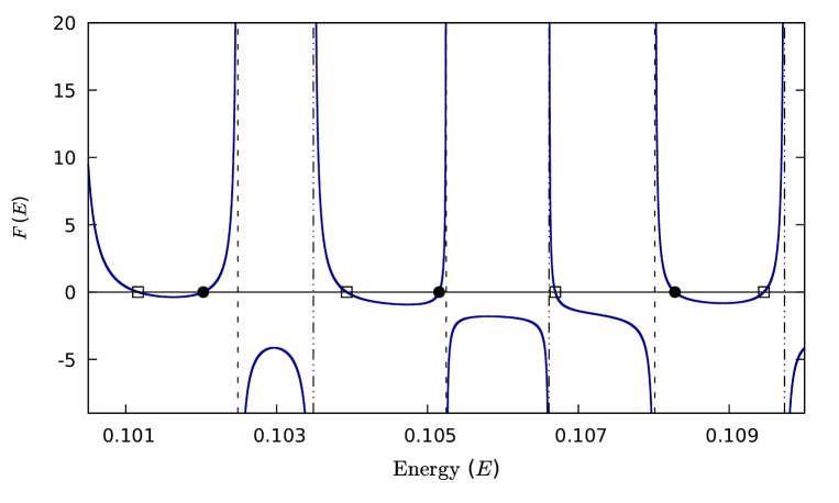
For a point in $\Sigma_{0,N}$, say $E^{0}_{m}$, we have $F(E^{0}_{m})=0$. Now assume $F^{\prime}(E^{0}_{m})>0$, then for $E$ slightly larger than $E^{0}_{m}$, $F(E)>0$ and according to the previous result $F^{\prime}(E)>0$. Therefore, $F(E)$ increases with $E$ until we encounter an eigenvalue of $H$ for $t_{0}=\infty$, say $E^{\infty}_{m^{\prime}}$. At this point $F(E)$ diverges. This implies that for each value of $t_{0}$ we have one and only one solution for the equation (12) with energy in the interval $[E^{0}_{m},E^{\infty}_{m^{\prime}}]$. In the case $F^{\prime}(E^{0}_{m})<0$ we have a similar result but now going down in energies in such a way that there is one and only one eigenstate of $H$ for each value of $t_{0}$ with energy in the interval $[E^{\infty}_{m^{\prime}},E^{0}_{m}]$, where $E^{\infty}_{m^{\prime}}$ is the point in $\Sigma_{\infty,N}$ immediately smaller than $E^{0}_{m}$. Finally, in the unlikely instance in which $F^{\prime}(E^{0}_{m})=0$ one necessarily has $f_{1}(E^{0}_{m})=f_{2}(E^{0}_{m})=0$ and therefore $F^{\prime\prime}(E^{0}_{m})=f^{\prime}_{1}(E^{0}_{m})f^{\prime}_{2}(E^{0}_{m})>0$. But this later property means that $F(E)>0$ for $E$ in a punctured neighbourhood of $E^{0}_{m}$, hence the arguments above hold and $F(E)$ grows monotonically to infinity when we separate from $E^{0}_{m}$ in both directions and approach the immediate points of $\Sigma_{\infty,N}$.

Due to this fact, we clearly see that given an interval of energies $I\subset(-t_{1},t_{1})$ the number of stationary states with energies in $I$ varies at most by two with $t_{0}$, namely

$$2\geq\sharp(I\cap\Sigma_{t_{0}})-\sharp(I\cap\Sigma_{0})\geq-2.$$

Therefore, the density of states $\lambda_{t_{0}}$ derived from (10) is independent of $t_{0}$ and, as we anticipated at the beginning of this section, it can be written as the sum of the densities for the two chains, i. e.

$$\lambda_{t_{0}}(E)=\frac{\nu_{1}/{\sqrt{t_{1}^{2}-E^{2}}}+\nu_{2}/{\sqrt{t_{2}^{2}-E^{2}}}}{\pi}.$$ (13)

For further purposes we also introduce the spectral density normalized in the interval of energies $(-t_{1},t_{1})$ in which the stationary states extend along the whole chain

$$\hat{\lambda}_{t_{0}}(E)=\frac{\nu_{1}/{\sqrt{t_{1}^{2}-E^{2}}}+\nu_{2}/{\sqrt{t_{2}^{2}-E^{2}}}}{\pi\nu_{1}+2\nu_{2}\arcsin(t_{1}/t_{2})}.$$

This result has been checked numerically and the results are presented in fig. 4. There the histogram for the energy of the states, determined numerically, is plotted against the theoretical curve obtained above. It is quite manifest the perfect agreement of both results.

Figure 4: In the histogram we represent the frequency of the spectrum with bins of width $0.01$ units of energy. The discontinuous line is the theoretical prediction obtained from (13).

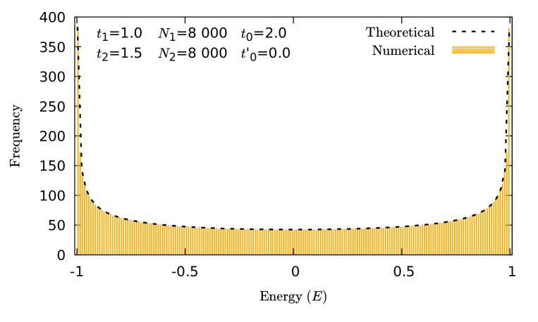
Notice that we have shown, in passing, that for $E\in(-t_{1},t_{1})$, $t_{0}\not=0$ or $\infty$ and $N$ large enough, there is no degeneracy in the spectrum of $H$. This is very good news because in the case of a degenerate eigenvalue the leaning of the eigenstates is not well defined; it means that the accidental degeneracy (and the undefinition of the leaning) can only possibly happen in the extreme cases $t_{0}=0$ or $\infty$, and this only after fine tunning $t_{1},t_{2}$ and $N$.

V Resonant regions

We turn now our attention to other feature of the plots in fig. 2: the existence of resonances.

We call resonant regions those windows in energy where the points in the plot accumulate at a few definite values of the leaning, like for instance in the central zone of the upper-left panel of fig. 2. Outside these regions the points $(E,{L}_{E})$ spread and the cloud seems to fill the whole allowed band. We have observed that the width of the resonances depends on $N$, in such a way that they shrink when $N$ grows.

To understand the reason for these facts let us consider a solution $E_{0}$ for (8)

$$C_{0}=\frac{t_{1}}{t_{0}}\frac{\sin((N_{1}+1){k}_{1}(E_{0}))}{\sin(N_{2}{k}_{2}(E_{0}))}=\frac{t_{0}}{t_{2}}\frac{\sin(N_{1}{k}_{1}(E_{0}))}{\sin((N_{2}+1){k}_{2}(E_{0}))},$$

and expand around this value

$$C_{0}+\Delta C=\frac{t_{1}}{t_{0}}\frac{\sin((N_{1}+1)({k}_{1}(E_{0})+{k}^{\prime}_{1}(E_{0})\Delta E+...))}{\sin(N_{2}({k}_{2}(E_{0})+{k}^{\prime}_{2}(E_{0})\Delta E+...))}$$ (14)

(15)

$$=\frac{t_{0}}{t_{2}}\frac{\sin(N_{1}({k}_{1}(E_{0})+{k}^{\prime}_{1}(E_{0})\Delta E+...))}{\sin((N_{2}+1)({k}_{2}(E_{0})+{k}^{\prime}_{2}(E_{0})\Delta E+...))}.$$ (16)

Now, writing $N_{i}=\nu_{i}N$ for some integer $N$ we impose the resonant condition

$$\frac{\nu_{1}{k}^{\prime}_{1}(E_{0})}{\nu_{2}{k}^{\prime}_{2}(E_{0})}=\frac{m_{1}}{m_{2}},\quad m_{1},m_{2}\in{\mathbb{Z}},$$

or in other words

$$m_{1}=r\,\nu_{1}{k}^{\prime}_{1}(E_{0}),\qquad m_{2}=r\,\nu_{2}{k}^{\prime}_{2}(E_{0}),\qquad\mbox{for some }r\in{\mathbb{R}},$$

where we have assumed that $m_{1}$ and $m_{2}$ are relative primes. Then, for large $N$, it is clear that if we take

$$\Delta E=\frac{\pi rn}{N},\quad n\in{\mathbb{Z}},$$

the first subleading terms in the expansion above (for $n=O(1)$) are

$$N_{i}{k}_{i}^{\prime}(E_{0})\Delta E=\pi m_{i}n$$

and one easily checks that $E_{0}+\Delta E$ is another solution of (8) up to corrections of order $O(1/N)$. The relevant fact is that these solutions give the same value for $C_{0}^{2}$, and therefore for the leaning, up to $O(1/N)$ terms. This explains the smooth curves of the Lissajous type that we observe for certain values of the energy.

To determine the width of the window we must consider the subleading corrections. They pose a limit to the validity of our approximation. To be specific let us focus in the argument of the first numerator in (14) and write

$$(N_{1}+1){k}_{1}(E_{0}+\Delta E) = (N_{1}+1){k}_{1}(E_{0})+N_{1}{k}^{\prime}_{1}(E_{0})\Delta E$$ (17)

$$+ {k}^{\prime}_{1}(E_{0})\Delta E+\frac{1}{2}N_{1}{k}^{\prime\prime}_{1}(E_{0})(\Delta E)^{2}+\dots$$ (19)

As we discussed before, given our choice of $\Delta E=\pi rn/N$ the second term of the expansion gives a contribution $\pi m_{1}n$ and hence, inside the sinus function reduces to a global $\pm 1$, which is the same at both sides of (8) and can be removed. The next two terms are

$$\frac{\pi rn}{N}{k}^{\prime}_{1}(E_{0})+\frac{\nu_{1}(\pi rn)^{2}}{2N}{k}^{\prime\prime}_{1}(E_{0}).$$

Note that for $n=O(\sqrt{N})$ the second term above is of order $O(1)$ and our approximation ceases to be valid. Hence we conclude that the width of the resonant windows scales like $1/\sqrt{N}$.

This is true provided ${k}_{1}^{\prime\prime}(E_{0})\not=0$ which does not hold at $E_{0}=0$. In this case we must go one step further in the expansion, so that the first corrections are

$$\frac{\pi rn}{N}{k}^{\prime}_{1}(0)+\frac{\nu_{1}(\pi rn)^{3}}{6N^{2}}{k}^{\prime\prime\prime}_{1}(0),$$

which are of order $O(1)$ for $n=O(N^{2/3})$ and the validity of our approach extends as far as $\Delta E=O(N^{-1/3})$. This explains why the resonances at the center of the plot, when they occur, are much wider.

A different question is: how many curves in the $E$-${L}$ plane are there around a resonant value $E_{0}$?, or in other words, how many well separated values for the leaning do we get for values of the energy near $E_{0}$? To answer this question we may use the results for the spectral density that we derived in the previous section.

First, consider that the separation between two consecutive values for the energy with the same value of the leaning (up to $O(1/N)$) is

$$\delta E=\pi r/N.$$

Now, combining this with the spectral density (13) we can obtain the number of states between two consecutive repetitions of the leaning, i. e. the number of curves at the outset of the resonance. Namely

$$N\lambda_{t_{0}}(E_{0})\delta E=N\frac{\nu_{1}{k}^{\prime}_{1}(E_{0})+\nu_{2}{k}^{\prime}_{2}(E_{0})}{\pi}\frac{\pi r}{N}=m_{1}+m_{2},$$

where for the last equality the conditions for resonance, $m_{i}=r\nu_{i}{k}^{\prime}_{i}(E_{0})$, have been used.

Then, we conclude that the number of curves that we obtain at the resonant value is precisely $m_{1}+m_{2}$. These results are illustrated in fig. 5 where we show the plot for the leaning and we superimpose some resonant values obtained according to our derivation. Note that the number of Lissajous type curves is also correctly predicted.

Figure 5: In these figures we show the plots of the leaning versus energy for different composed systems with the hopping, sizes and contacts that appear in every panel. The vertical lines mark the value of the energy for which we expect a resonance according to the discussion in section V. The pair of numbers at every vertical line is the theoretical relation between the two resonant frequencies. Notice that the number of Lissajous type curves at every resonance coincides with the sum of those two numbers, as it is explained in the text.

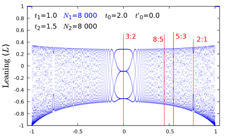
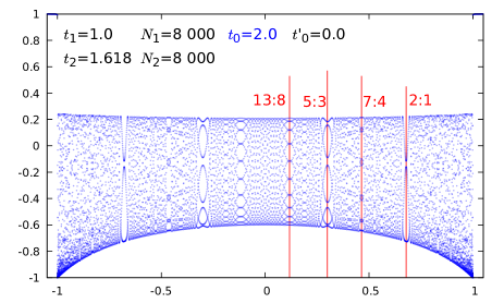
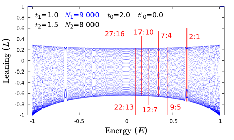
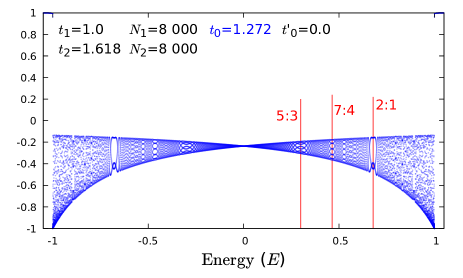
We must add that at some special points, like for instance at $E_{0}=0$, there may appear some degeneracy for the leaning which results in a smaller number of different values for it. This is clearly observed in the upper-left panel of fig. (5), where the crossing of the curves at $E_{0}=0$ reduces from five to three the number of allowed values for the leaning. Of course, this degeneracy occurs only at $E_{0}=0$ and is broken in its vicinity, recovering there the right number of curves.

As it is clear from the plots and from the discussion in this section, the resonance windows do not depend on the contact $t_{0}$ of the two subsystems but they are sensitive to its size. In the next section we will discuss a property of the plots that behaves exactly in the opposite way, i. e. it is independent of the size and varies with the contact coupling $t_{0}$.

VI The boundary.

In this section, we will find an analytical expression for the curves that limit the distribution of points in the $E$-${L}$ plane.

We are interested in the boundaries of the cloud in the $E$-${L}$ plane that are valid in the thermodynamic limit, when $N_{1},N_{2}\to\infty$. To achieve this goal we first look for an upper and lower bound of $C^{2}$ at a given value of the energy. It is clear that, given the monotonic decreasing character of the leaning in (9) with $C^{2}$, the latter leads respectively to lower and upper bounds for ${L}$.

It also happens that, as we show below, it is possible to obtain bounds for $C^{2}$ which are valid for any $N_{1},N_{2}$ and are optimal, in the sense that they can be approached as much as we want by varying the size of the two parts of the system.

As we look for bounds for $C^{2}$ independent of $N_{1},N_{2}$, it makes sense to replace $N_{1}{k}_{1}(E)$ and $N_{2}{k}_{2}(E)$ inside the trigonometric functions of (8) by two continuous variables $\xi_{1},\xi_{2}\in[0,2\pi)$ independent, in principle, of $E$.

To justify this replacement consider, on the one hand side, that we are looking for bounds for $C^{2}$, then if we relax the conditions for the equation (8) we are sure that the bounds for the modified equation are still valid for the original one. On the other hand, we may argue that by considering $N_{i}$ large enough we may approach any value $\xi_{i}$ as much as we want which implies that our bounds, valid for any $N_{i}$, are optimal.

To proceed, we replace the equation (8) by

$$\frac{t_{1}}{t_{0}}\frac{\sin(\xi_{1}+{k}_{1}(E))}{\sin\xi_{2}}=\frac{t_{0}}{t_{2}}\frac{\sin\xi_{1}}{\sin(\xi_{2}+{k}_{2}(E))},$$ (20)

and, consequently,

$$C^{2}=\frac{t^{2}_{1}}{t^{2}_{0}}\frac{\sin^{2}(\xi_{1}+{k}_{1}(E))}{\sin^{2}\xi_{2}}.$$ (21)

If we replace $\xi_{i}$ by the new variables

$$z_{i}=\cos{k}_{i}(E)+\sin{k}_{i}(E)\cot\xi_{i},\quad i=1,2,$$

then equation (20) is easily solved

$$z_{2}=\frac{t_{0}}{\bar{t}_{0}}z_{1}^{-1},$$

where for later convenience we have introduced the dual contact $\bar{t}_{0}=t_{1}t_{2}/t_{0}$. Now we use the previous relation to express $C^{2}$ in terms of the single variable $z_{1}$ to obtain

$$C^{2}=\frac{\sin^{2}{k}_{1}}{t_{2}^{2}\sin^{2}{k}_{2}}\frac{\bar{t}_{0}^{2}z_{1}-2t_{0}\bar{t}_{0}\cos{k}_{i}+t_{0}z_{1}^{-1}}{\bar{z}_{1}-2\cos{k}_{i}+z_{1}^{-1}}.$$ (22)

Then, we simply have to determine the maximum and minimum of (22) as a function of $z_{1}$, for every value of the energy. The task is, of course, straightforward but somehow painful. The final expressions are rather cumbersome and of little interest to us. Instead of writing down the analytic expression for the upper and lower bound of $C^{2}$ and the leaning, we prefer to plot it for some special cases.

Notice that, as the bounds for $C^{2}$ are independent of $N_{1},N_{2}$, those of ${L}$ only depend on $\nu_{1}$ and $\nu_{2}$, namely

$${L}=\frac{\nu_{1}C^{2}-\nu_{2}}{\nu_{1}C^{2}+\nu_{2}}.$$

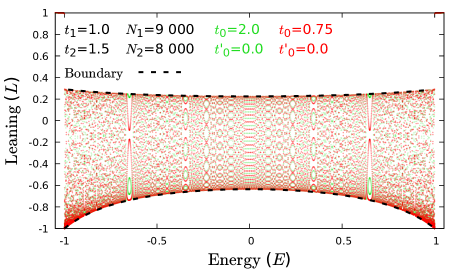
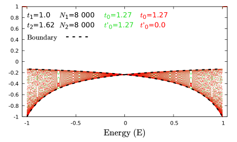
The comparison between the analytic and numerical results for different relative sizes and values of the contact are collected in the plots of fig. 6.

Figure 6: In these plots we show the distribution for the leaning versus the energy of different chains. In the left panel the two systems are related by duality $t_{0}\leftrightarrow t_{1}t_{2}/t_{0}$. It is clear that although the two distributions of points (represented in different colors) are not identical they fill the same region. In the panel on the right we represent the selfdual case $t_{0}=\sqrt{t_{1}t_{2}}$ and the two distributions differ by the largest contact $t^{\prime}_{0}$. The situation is similar to the previous one, different distribution but the same boundaries. The discontinuous lines represent the theoretical boundaries obtained as explained in the text.

An interesting fact that we would like to emphasize is the duality between higher and lower contact. In fact, we can show that the bounds are unchanged if we replace $t_{0}$ by

$$\bar{t}_{0}=t_{1}t_{2}/t_{0}.$$

A duality that maps zero to infinity or, as we mentioned above, higher to lower coupling constant.

The duality is easily proven starting from (22). There we see that the value of $C^{2}$ is unchanged if we replace $t_{0}$ by $\bar{t}_{0}$ and simultaneously $z_{1}$ by $z_{1}^{-1}$. Therefore, the maximum and minimum for $C^{2}$ are unchanged under the duality.

In the left panel of fig. 6, we plot the leaning for dual values of the contact and we see that the respective allowed regions perfectly match. On the right side of this figure, the leaning for a self dual value of the contact $t_{0}=\sqrt{t_{1}t_{2}}$ is plotted.

Let us discuss now which is the effect of taking $t^{\prime}_{0}\not=0$. First notice that if we replace in (4) $\delta_{i}$ by $\delta_{i}-N_{i}{k}_{i}(E)/2,\ i=1,2$, which is a simple redefinition of the unknowns, we obtain a more symmetric equation. Actually, replacing now $\delta_{i}+N_{i}{k}_{i}/2$ by $\xi_{i}$ and $N_{i}{k}_{i}/2-\delta_{i}-{k}_{i}$ by $\eta_{i}$ we obtain the equivalent equations:

$$C=\frac{t_{1}}{t_{0}}\frac{\sin(\xi_{1}+{k}_{1}(E))}{\sin\xi_{2}}=\frac{t_{0}}{t_{2}}\frac{\sin\xi_{1}}{\sin(\xi_{2}+{k}_{2}(E))},$$ (23)

$$C=\frac{t_{1}}{t^{\prime}_{0}}\frac{\sin(\eta_{1}+{k}_{1}(E))}{\sin\eta_{2}}=\frac{t^{\prime}_{0}}{t_{2}}\frac{\sin\eta_{1}}{\sin(\eta_{2}+{k}_{2}(E))}.$$ (24)

Notice that the second line is like the first one by simply replacing $\xi$ by $\eta$ and $t_{0}$ by $t_{0}^{\prime}$. Then we have two equations for obtaining bounds on $C^{2}$, one with $t_{0}$ and another with $t_{0}^{\prime}$. It happens that the smaller $t_{0}+\overline{t}_{0}$ is (its minimum value is attained for the selfdual case $t_{0}=\sqrt{t_{1}t_{2}}$) the more restrictive the bounds are, and this applies both for the upper and the lower bound.

Consequently, only one of the contacts matters for determining the boundaries of the allowed region in the $E$-${L}$ plane, namely the one closer to the selfdual value or equivalently the one with the least value for $t_{0}+\overline{t}_{0}$.

More formally, if we introduce an order relation defined by: $t_{0}\prec t_{0}^{\prime}$ if and only if $t_{0}+\overline{t_{0}}<t^{\prime}_{0}+\overline{t^{\prime}_{0}}$, the smallest of the two contacts determines the shape of the cloud.

This can be checked in the numerical experiments where it is apparent that a modification of the larger contact does not alter the shape of the cloud, as can actually be seen in the right plot of fig. 6.

VII The probability measure

If we examine the different plots of previous sections, one observes that for most of the allowed region the points that represent $(E,{L})$ pairs form a cloud more dense near the boundaries and more sparse at the middle. Of course, the previous is not true at the resonance windows, where the points form definite curves. But, as we discussed in section V, one can prove that the resonant regions shrink with the size of the system and eventually disappear in the thermodynamic limit.

Then the question that might have sense and we will study is whether there is a measure in the $E$-${L}$ plane that represents the density of points in the thermodynamic limit and how it depends on the parameters of the system. We believe that such a measure exists and for $t_{0},t^{\prime}_{0}\not=0$ is absolutely continuous with respect to the Lebesgue measure.

To be more precise, take $N_{1}=\nu_{1}N$ and $N_{2}=\nu_{2}N$, let the hopping parameters be as usual $t_{2}>t_{1}>0$ and contacts $t_{0},t_{0}^{\prime}$. Now we define the following probability measure on the Borelians $S\subset X=[-t_{1},t_{1}]\times[-1,1]$

$$\mu_{N}(S)=K_{N}\,\sharp\{\Psi_{E}\,|\,(E,L_{E})\in S\},$$

where by $\sharp$ we denote the cardinality of the set, $\Psi_{E}$ is an eigenfunction of the Hamiltonian of the composite system with chains of length $\nu_{1}N$ and $\nu_{2}N$, and ${L}_{E}$ is the leaning of $\Psi_{E}$. $K_{N}$ is the appropriate normalization constant to obtain a probability measure, i. e. $\mu_{N}(X)=1$.

We assert that these measures converge, when $N\to\infty$, to a probability measure $\mu$ on the Borelians of $X$.

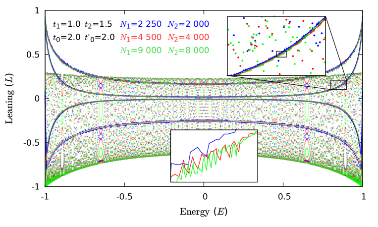
We do not have a proof for the existence of $\mu$, only numerical evidences based on the good behaviour of the expected value for different random variables and its apparent convergence with $N$ as illustrated in fig. 7. There we show the plot of the leaning for different values of $N_{1}$ and $N_{2}$ with the same relative sizes $N_{1}/N_{2}$ and the running average $\langle L^{n}\rangle$ for $n=1$ that corresponds to the lowest (blurry) curve and going upwards $n=7,6,2$. We see that the curves for different sizes of the system agree to a large extent and they seem to have a smooth large $N$ limit. The well defined limit for the different moments is a strong numerical indication of the existence of a Borelian measure when $N\to\infty$.

Figure 7: In this plot we represent the distribution of points in the $L-E$ plane for chains that differ in size, while sharing the proportion between the two subsystems. Every size is represented in a different color. The curves are the running average (over 200 points) of $L^{n}$ for $n=1,7,6,2$ respectively from bottom to top. It is clear that the curves for different size almost coincide and the two consecutive magnification insets indicate that a well defined limit for the expectation value of all momenta, when $N\to\infty$, seems to exist.

Sometimes it will be important to emphasize the dependence of the limiting measure on some of the parameters of the theory, in that case we will write those parameters as subindices. In the following, we will focus mainly on the dependence of $\mu_{N}$ or $\mu$ on the contacts, so we will write it $\mu_{N,t_{0},t^{\prime}_{0}}$ or $\mu_{t_{0},t^{\prime}_{0}}$. The first observation is that due to the parity invariance of the Hamiltonian $\mu_{N,t_{0},t^{\prime}_{0}}=\mu_{N,t^{\prime}_{0},t_{0}}$; therefore, if the limit exists we must have $\mu_{t_{0},t^{\prime}_{0}}=\mu_{t^{\prime}_{0},t_{0}}$.

In general, we do not know how to determine $\mu_{t_{0},t_{0}^{\prime}}$, only when $t_{0}=t^{\prime}_{0}=0$ (or $\infty$) because, in this case, the chain splits into two independent homogeneous systems with well defined leaning. Therefore, $\mu_{0,0}$ can be obtained as the normalized sum of the corresponding spectral measures. Hence, we have

$${\rm d}\mu_{0,0}=\big{(}\rho_{1}(E)\delta({L+1})+\rho_{2}(E)\delta(L-1)\big{)}{\rm d}E\,{\rm d}L,$$

where

$$\rho_{i}(E)=\frac{\nu_{i}/\sqrt{t_{i}^{2}-E^{2}}}{\pi\nu_{1}+2\nu_{2}\arcsin(t_{1}/t_{2})},$$

and $\delta$ represents the Dirac delta function. That is, in this case the measure is supported in the upper and lower boundary of $X$, with $L=\pm 1$.

As we said, except for this trivial case, we are not able to determine $\mu$. However, based on numerical experiments and some analytical hints we can establish some conjectures that we present now.

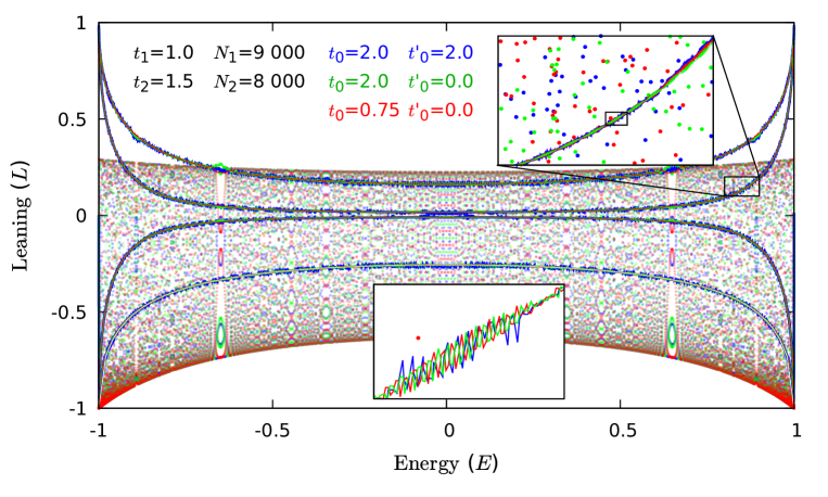
• According to the discussion of section VI, the support of the measure is in the region between the curves $L_{\rm max}(E),L_{\rm min}(E)$. Moreover, we proved in that section that the limiting curves depend only on the smallest contact i. e. they depend only on $t_{0}$ provided $t_{0}\prec t^{\prime}_{0}$. The stronger conjecture, suggested by different numerical experiments shown in fig. 8, is that not only the support of the measure depends only on the lowest contact, but the measure itself has the same property i. e. we conjecture

  $$\mu_{t_{0},t_{0}^{\prime}}=\mu_{t_{0},t_{0}^{\prime\prime}},\quad{\rm if}\ t_{0}\prec t^{\prime}_{0},t^{\prime\prime}_{0}.$$

  For this reason, and in order to simplify the notation, from now on we will refer to the measure writing only the smallest contact $\mu_{t_{0}}$.

• Another property of the limiting curves that we showed in section VI is its invariance under duality $t_{0}\mapsto\bar{t}_{0}=t_{1}t_{2}/t_{0}$. Based again in numerical evidences, see fig. 8 for an example, we conjecture

  $$\mu_{t_{0}}=\mu_{{\bar{t}_{0}}}.$$

  That is, we assert that not only the support of the measure is left invariant under the duality transformation, but also the measure itself.

We do not have any analytic argument to substantiate these two last properties. But if we compute the running moments in ${L}$ of the distributions, when varying $t^{\prime}_{0}$ or when replacing $t_{0}$ by $\overline{t}_{0}$, we find that they are as close as they possibly could be. This is shown in fig. 8.

Figure 8: In this plot we show the distribution of points and running average of the momenta $L^{n}$ ($n=1,7,6,2$ respectively for the curves from bottom to top) for three different chains. They differ by the value of $t^{\prime}_{0}=2.0$ or $0.0$ and/or by the replacement of $t_{0}=2$ by its dual value $t_{1}t_{2}/t_{0}=0.75$. We see that in this case the running average of the three different chains coincide. This coincidence is more striking if we look at the two consecutive magnifying insets.

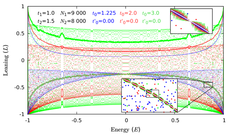
• From the dependence of the clouds with $t_{0}$, illustrated in fig. 9, it seems reasonable to conjecture that, except for $t_{0}=t^{\prime}_{0}=0$ (or $\infty$), the measure is absolutely continuous with respect to the Lebesgue measure. That is, there is a function $\sigma_{t_{0}}\in L^{1}(X)$ such that

  $${\rm d}\mu_{t_{0}}=\sigma_{t_{0}}(E,L)\,{\rm d}E\,{\rm d}L.$$

• Although we can not determine $\mu_{t_{0}}$, based on the arguments of section IV we believe that the marginal distribution for $E$ does not depend on $t_{0}$. Therefore, we can write

  $$\hat{\lambda}_{t_{0}}(E)\equiv\int_{-1}^{1}\sigma_{t_{0}}(E,{L}){\rm d}{L}=\frac{\nu_{2}/{\sqrt{t_{2}^{2}-E^{2}}}+\nu_{1}/{\sqrt{t_{1}^{2}-E^{2}}}}{2\nu_{2}\arcsin(t_{1}/t_{2})+\nu_{1}\pi},$$

  where the right hand side has been computed using the spectral density obtained in section IV or, alternatively, the measure that we determined before for $t_{0}=0$.

• Finally, we can prove that the expected value of $L$ at fixed value of the energy is also independent of $t_{0}$. Indeed, using again the probability measure at $t_{0}=0$, we have

  $$\langle{L}\rangle_{E}\equiv\hat{\lambda}_{t_{0}}(E)^{-1}\int_{-1}^{1}\sigma_{t_{0}}(E,{L}){L}{\rm d}{L}=\frac{\nu_{2}/{\sqrt{t_{2}^{2}-E^{2}}}-{\nu_{1}}/{\sqrt{t_{1}^{2}-E^{2}}}}{\nu_{2}/{\sqrt{t_{2}^{2}-E^{2}}}+{\nu_{1}}/{\sqrt{t_{1}^{2}-E^{2}}}}.$$ (25)

  As it is explained in the appendix, this result can be proven by estimating the running average of $L$ in the large $N$ limit. Numerical experiments also support our result. These are shown in fig. 9 where we present the running average of the leaning that we obtained numerically for different values of $t_{0}$ (the thick curve transversing the cloud in its lower part), and we check that it is independent of $t_{0}$ and agrees extremely well with the conjectured predictions. If we look at the two magnifying insets it is clear that curves for different $t_{0}$, represented in different colors, agree perfectly. They also coincide with the theoretical value of (25) that we plot in white and is the line that cuts right in the middle the numerical curves. In contrast, the numerical curves for $\langle L^{2}\rangle$ for different values of $t_{0}$ (in different colors, in the upper part of the plot) are well separated.

Figure 9: In this plot we show the distribution of points and running average $\langle L\rangle$ and $\langle L^{2}\rangle$, over 200 points, for chains that differ in the contact, $t_{0}$, and are represented in different colors. While the three curves corresponding to $\langle L^{2}\rangle$ are clearly different, those for $\langle L\rangle$ coincide as it is made manifest in the insets. The curve in white (visible in the insets) represents the predicted value. The explanation for this fact is presented in the appendix.

VIII Conclusions, generalizations and extensions

We have shown that the probability of presence for one particle in a composite system, characterized here with the leaning, follows a rather intricate pattern.

We have been able to unravel many of its properties, like the nature of the resonant regions, the boundaries of the allowed region, its independence of the largest contact, the duality between large and small contact coupling or the universal properties of the average leaning.

It is interesting to remark that the leaning, in the thermodynamic limit, is definitely a non perturbative property. This can be argued in several ways: first, the duality discussed in sections VI and VII and mentioned above allows to identify the small and large coupling constant region $t_{0}\leftrightarrow t_{1}t_{2}/t_{0}$; second, we observe that for no matter how little $t_{0}\not=0$ is we may find (for $N$ large enough) states with a leaning arbitrary close to $0$, very far from the unperturbed system where $|L|=1$ for any state.

Suggestively enough, the non perturbative character of the leaning can be traced back to the existence (for large $N$) of small denominators in the quantum perturbative expansion. This is reminiscent of the same phenomena in the canonical perturbation expansion in classical mechanics, which is one of the essential ingredients for the existence of non integrable systems and chaotic dynamics.

Here, of course, we may not have sensitive dependence on initial conditions for the evolution, as the dynamics is linear; but, instead, the expected position of one particle stationary states depends sensitively on its energy.

While, as we just stated, the leaning depends critically on the energy of the stationary state, we may obtain a predictable result if we consider the average over a range of energy. This is observed numerically and can be rigorously proven. For the latter proof we have to get rid of the small denominators problem and it is interesting to remark that the way we proceed is very much reminiscent of the analogous strategy for the proof of KAM theorem in classical perturbation theory: we fix initially a cut-off that suppresses the small denominators, then we can proceed with the different estimates before removing the cut-off.

An open problem is to compute the density in the $E$-$L$ plane for the stationary states in the thermodynamic limit. There are strong numerical indications that such a Borelian measure exists, it is absolutely continuous with respect to the Lebesgue measure (except for $t_{0}$ and $t_{0}^{\prime}$ equal to $0$ or $\infty$) and varies continuously with $t_{0}$ in the total variation topology (the convergence for $t_{0},t_{0}^{\prime}\to 0,\infty$ should occur only in the weak topology).

Let us remark that the previous results were obtained for the simplest kind of systems composed of two homogeneous tight-binding chains joined at every end by links with different hopping parameter. However, the behaviour that we have described in the paper seems rather universal and it has been observed for the SSH chain (alternating hopping), for the Ising chain and, more generally, for the $XY$ spin chain. One can consider also different types of contacts (of finite range) without affecting the essential properties of the leaning. Particular examples beyond tight binding models will be presented elsewhere.

Another interesting issue connected to this paper is the continuum limit of our system (different from the thermodynamic limit that we work out here). The natural guess is a free fermion in one dimension with boundary conditions, impurities and/or localized (delta like) potentials. At present we do not know if a similar pattern for the leaning in this kind of systems occurs. This is a very interesting question and it could help to clarify the weak/strong coupling duality that we uncover in this work. In fact, for a free fermion, the latter can be explained by the existence of dualities in the bosonization process. A similar explanation could also be valid here.

Finally, we would like to comment that all the systems mentioned so far can be mapped to free fermionic chains and therefore can be analyzed with relatively ease. It would be interesting to go beyond that and explore the behaviour of the leaning for systems composed of interacting chains like the Hubbard model or others. We plan to approach these problems in our future research.

Acknowledgments: Research partially supported by grants E21 17R, DGIID- DGA, and PGC2018-095328-B-100, MINECO (Spain). FA is supported by Brazilian Ministries MEC and MCTIC and acknowledges the warm hospitality and support of Departamento de Física Teórica, Universidad de Zaragoza, during several stages of this work. We would like to acknowledge one of the referees for interesting remarks concerning the continuum limit.

Appendix A

In this appendix, we present a proof of the invariance of the leaning average under a change of the contact.

More precisely, given a fermionic chain like the one described in section II ($0<t_{1}<t_{2}$ and, for simplicity, $t_{0}^{\prime}=0$) we compute the running average of the leaning in an interval of energy $[E-\Delta E,E+\Delta E]\subset(-t_{1},t_{1})$.

For that, let us denote the spectra for contact $t_{0}$ and $0$ respectively by $\Sigma_{t_{0},N}=\{E_{m};m\in M\}$ and $\Sigma_{0,N}=\{E^{0}_{\widetilde{m}};\widetilde{m}\in M_{0}\}$ as before, and the normalized eigenstates by $\psi_{m}$ and $\varphi_{\widetilde{m}}$ respectively. Introduce $R\subset M$ such that

$$\{E_{m};m\in R\}=\Sigma_{t_{0},N}\cap[E-\Delta E,E+\Delta E],$$

and similarly $R_{0}\subset M_{0}$ for $\Sigma_{0,N}\cap[E-\Delta E,E+\Delta E]$. With these data we define the density matrices

$$\rho=\frac{1}{\sharp\,(R)}\sum_{m\in R}\mathinner{|{\psi_{m}}\rangle}\mathinner{\langle{\psi_{m}}|},$$

and

$$\rho_{0}=\frac{1}{\sharp\,(R_{0})}\sum_{\widetilde{m}\in R_{0}}\mathinner{|{\varphi_{\widetilde{m}}}\rangle}\mathinner{\langle{\varphi_{\widetilde{m}}}|}.$$

We will prove that in the thermodynamic limit

$$\lim_{N\to\infty}{\rm Tr}\left((\rho-\rho_{0})(P_{2}-P_{1})\right)=0.$$

Or in other words, the leaning averaged over a range of energy does not depend on the contact in the thermodynamic limit.

To show it we express $\rho$ in terms of the unperturbed basis,

$$\rho=\frac{1}{\sharp\,(R)}\sum_{r\in R}\sum_{\widetilde{m},\widetilde{m}^{\prime}\in M_{0}}U_{\widetilde{m},r}\overline{U}_{\widetilde{m}^{\prime},r}\mathinner{|{\varphi_{\widetilde{m}}}\rangle}\mathinner{\langle{\varphi_{\widetilde{m}^{\prime}}}|},$$

where $U$ is the unitary matrix corresponding to the change of basis, that is $U_{\widetilde{m},r}=\mathinner{\langle{\varphi_{\widetilde{m}}}|{\psi_{r}}\rangle}$.

Now we decompose the sets of indices into two disjoint sets, $M=R\cup P$ and $M_{0}=R_{0}\cup P_{0}$, and write

$$\rho = \frac{1}{\sharp\,(R)}\sum_{r\in R}\left(\sum_{\widetilde{r},\widetilde{r}^{\prime}\in R_{0}}U_{\widetilde{r},r}\overline{U}_{\widetilde{r}^{\prime},r}\mathinner{|{\varphi_{\widetilde{r}}}\rangle}\mathinner{\langle{\varphi_{\widetilde{r}^{\prime}}}|}+\sum_{\widetilde{r}\in R_{0},\widetilde{p}\in P_{0}}U_{\widetilde{r},r}\overline{U}_{\widetilde{p},r}\mathinner{|{\varphi_{\widetilde{r}}}\rangle}\mathinner{\langle{\varphi_{\widetilde{p}}}|}+\right.$$ (27)

$$\hskip 51.21504pt\left.\sum_{\widetilde{r}\in R_{0},\widetilde{p}\in P_{0}}U_{\widetilde{p},r}\overline{U}_{\widetilde{r},r}\mathinner{|{\varphi_{\widetilde{p}}}\rangle}\mathinner{\langle{\varphi_{\widetilde{r}}}|}+\sum_{\widetilde{p},\widetilde{p}^{\prime}\in P_{0}}U_{\widetilde{p},r}\overline{U}_{\widetilde{p}^{\prime},r}\mathinner{|{\varphi_{\widetilde{p}}}\rangle}\mathinner{\langle{\varphi_{\widetilde{p}^{\prime}}}|}\right).$$

Due to the orthonormality properties of $U$ we can rewrite the first term as

$$\sum_{r\in R}\sum_{\widetilde{r},\widetilde{r}^{\prime}\in R_{0}}U_{\widetilde{r},r}\overline{U}_{\widetilde{r}^{\prime},r}\mathinner{|{\varphi_{\widetilde{r}}}\rangle}\mathinner{\langle{\varphi_{\widetilde{r}^{\prime}}}|}=\sum_{\widetilde{r}\in R_{0}}\mathinner{|{\varphi_{\widetilde{r}}}\rangle}\mathinner{\langle{\varphi_{\widetilde{r}}}|}-\sum_{p\in P}\sum_{\widetilde{r},\widetilde{r}^{\prime}\in R_{0}}U_{\widetilde{r},p}\overline{U}_{\widetilde{r}^{\prime},p}\mathinner{|{\varphi_{\widetilde{r}}}\rangle}\mathinner{\langle{\varphi_{\widetilde{r}^{\prime}}}|}.$$

With the above replacement and taking into account that the stationary states of the unperturbed Hamiltonian are also eigenstates of the leaning operator:

$$(P_{2}-P_{1})\varphi_{\widetilde{m}}=\epsilon_{\widetilde{m}}\,\varphi_{\widetilde{m}}\ \mbox{ with }\ \epsilon_{\widetilde{m}}=\pm 1,$$

we can write

$$\mathop{\mbox{Tr}}\nolimits(\rho(P_{2}-P_{1})) = \frac{\sharp(R_{0})}{\sharp(R)}\mathop{\mbox{Tr}}\nolimits(\rho_{0}(P_{2}-P_{1}))$$ (29)

$$+\frac{1}{\sharp(R)}\left(\sum_{\widetilde{p}\in P_{0},r\in R}\epsilon_{\widetilde{p}}|U_{\widetilde{p}r}|^{2}-\sum_{\widetilde{r}\in R_{0},p\in P}\epsilon_{\widetilde{r}}|U_{\widetilde{r}p}|^{2}\right).$$

Now we must estimate the matrix elements of $U$. This can be done by means of the identity

$$|U_{\widetilde{m}m}|^{2}=\frac{|\mathinner{\langle{\varphi_{\widetilde{m}}}|}H_{I}\mathinner{|{\psi_{m}}\rangle}|^{2}}{(E^{0}_{\widetilde{m}}-E_{m})^{2}},$$ (30)

where we can take advantage of the fact that $\varphi_{\widetilde{m}}$ and $\psi_{m}$ are extended wave functions and $H_{I}$ acts only locally at the interface of the two components of the chain. Indeed, one has

$$|\mathinner{\langle{\varphi_{\widetilde{m}}}|}H_{I}\mathinner{|{\psi_{m}}\rangle}|=O(N^{-1}).$$

The problem, however, is that the denominator $(E^{0}_{\widetilde{m}}-E_{m})^{2}$ for large $N$ and particular values of $m$ and $\widetilde{m}$ can be very small (even smaller than $1/N^{2}$). This is an instance of the small denominator problem in quantum mechanics.

To avoid this potential divergence we must introduce a cut-off. A similar strategy (although much simpler in this case) to the one followed for proving the KAM theorem in classical mechanics.

For instance, to estimate the second term in (29),

$$|F|\equiv\frac{1}{\sharp(R)}\bigg{|}\sum_{\widetilde{p}\in P_{0},r\in R}\epsilon_{\widetilde{p}}|U_{\widetilde{p}r}|^{2}\bigg{|}\leq\frac{1}{\sharp(R)}\sum_{\widetilde{p}\in P_{0},r\in R}|U_{\widetilde{p}r}|^{2},$$

we fix a range of energy $\delta E<\Delta E$ and decompose the set $R$ into two disjoint subsets $R=R_{<}\cup R_{>}$ with

$$R_{<}=\{r\in R\mbox{ s. t. }|E_{r}-E|<\Delta E-\delta E\},$$

which implies that $|E_{\widetilde{p}}-E_{r_{{}_{<}}}|>\delta E$, for any $\widetilde{p}\in P_{0},r_{{}_{<}}\in R_{<}$, and the small denominator problem is relegated to the set of indices $R_{>}$.

Thus we have

$$|F| \leq \frac{1}{\sharp(R)}\left(\sum_{\widetilde{p}\in P_{0},r_{{}_{>}}\in R_{>}}|U_{\widetilde{p}r_{{}_{>}}}|^{2}+\sum_{\widetilde{p}\in P_{0},r_{{}_{<}}\in R_{{}_{<}}}|U_{\widetilde{p}r_{{}_{<}}}|^{2}\right)$$ (31)

$$\leq \frac{\sharp(R_{>})}{\sharp(R)}+\frac{1}{\sharp(R)}\sum_{\widetilde{p}\in P_{0},r_{{}_{<}}\in R_{<}}\frac{|\mathinner{\langle{\varphi_{\widetilde{p}}}|}H_{I}\mathinner{|{\psi_{r_{{}_{<}}}}\rangle}|^{2}}{(\delta E)^{2}},$$ (32)

where we have used the normalization condition for the rows of $U$ to estimate the first term and (30) together with the bound for the energy difference for the second.

Now

$$\sum_{\widetilde{p}\in P_{0}}|\mathinner{\langle{\varphi_{\widetilde{p}}}|}H_{I}\mathinner{|{\psi_{r_{{}_{<}}}}\rangle}|^{2}\leq\mathinner{\langle{\psi_{r_{{}_{<}}}}|}H_{I}^{2}\mathinner{|{\psi_{r_{{}_{<}}}}\rangle}\leq\frac{2t_{0}^{2}}{M},$$

with

$$M=\min\left\{\nu_{1}N-\frac{t_{1}^{2}}{\sqrt{t_{1}^{2}-(|E|+\Delta E)^{2}}},\nu_{2}N-\frac{t_{2}^{2}}{\sqrt{t_{2}^{2}-(|E|+\Delta E)^{2}}}\right\}.$$

The important fact here is that for fixed $|E|+\Delta E<t_{1}<t_{2}$ we have $M=O(N)$ for large $N$.

Inserting this into (31) and performing the sum, we obtain

$$|F|\leq\frac{\sharp(R_{>})}{\sharp(R)}+\frac{2t_{0}^{2}}{M(\delta E)^{2}}.$$

The same estimate can be used for the third term on the right hand side of (29) to get

$$|\mathop{\mbox{Tr}}\nolimits((\rho-\rho_{0})(P_{2}-P_{1}))|\leq\frac{|\sharp(R_{0})-\sharp(R)|}{\sharp(R)}|\mathop{\mbox{Tr}}\nolimits(\rho_{0}(P_{2}-P_{1}))|+2\frac{\sharp(R_{>})}{\sharp(R)}+\frac{4t_{0}^{2}}{M(\delta E)^{2}}.$$ (33)

From the spectrum of $H_{0}$ we derive

$$\sharp(R_{0})\geq\frac{N}{\pi}\left(\frac{\nu_{1}}{t_{1}}+\frac{\nu_{2}}{t_{2}}\right)\Delta E-1,$$

and, from the results in section IV, we have

$$|\sharp(R_{0})-\sharp(R)|\leq 2.$$

Likewise we can obtain the upper bound

$$\sharp(R_{>})\leq\frac{N}{\pi}\left(\frac{\nu_{1}}{\sqrt{t_{1}^{2}-(|E|+\Delta E)^{2}}}+\frac{\nu_{2}}{\sqrt{t_{2}^{2}-(|E|+\Delta E)^{2}}}\right)\delta E+2.$$

Using the previous estimates and choosing the cutoff such that

$$\delta E\to 0,\mbox{ but }N(\delta E)^{2}\to\infty,\mbox{ when }N\to\infty,$$

e. g. $\delta E=N^{-1/3}$, we obtain from (33)

$$\lim_{N\to\infty}\mathop{\mbox{Tr}}\nolimits((\rho-\rho_{0})(P_{2}-P_{1}))=0,$$

as stated before.

References

- (1) G. Vidal, J.I. Latorre, E. Rico, A. Kitaev, Entanglement in quantum critical phenomena, Phys. Rev. Lett. 90, 22: 227902-227906 (2003), arXiv:quant-ph/0211074v1
- (2) B-Q. Jin, V.E. Korepin, Quantum Spin Chain, Toeplitz Determinants and Fisher-Hartwig Conjecture, J. Stat. Phys. 116 (2004) 157-190, arXiv:quant-ph/0304108
- (3) F. Ares, J. G. Esteve, F. Falceto, E. Sánchez-Burillo, Excited state entanglement in homogeneous fermionic chains, J. Phys. A: Math. Theor. 47 (2014) 245301, arXiv:1401.5922 [quant-ph]
- (4) F. Ares, J. G. Esteve, F. Falceto, Entanglement of several blocks in fermionic chains, Phys. Rev. A 90, (2014) 062321, arXiv:1406.1668 [quant-ph]
- (5) F. Ares, J. G. Esteve, F. Falceto, A. R. de Queiroz, Entanglement in fermionic chains with finite range coupling and broken symmetries, Phys. Rev. A 92, (2015) 042334, arXiv:1506.06665 [quant-ph]; Entanglement entropy in the Long-Range Kitaev chain, Phys. Rev. A 97, (2018) 062301, arXiv:1801.07043 [quant-ph]
- (6) F. Ares, J. G. Esteve, F. Falceto, Z. Zimborás, Sublogarithmic behaviour of the entanglement entropy in fermionic chains, J. Stat. Mech. (2019) 093105, arXiv:1902.07540 [cond-mat.stat-mech]
- (7) L. Amico, R. Fazio, A. Osterloh, V. Vedral, Entanglement in quantum many-body systems, Rev. Mod. Phys. 80, 517 (2008), arXiv:quant-ph/0703044
- (8) N. Laflorencie, Quantum entanglement in condensed matter systems, Phys. Rep. 643, 1 (2016), arXiv:1512.03388 [cond-mat.str-el]
- (9) J. Asbóth, L. Oroszlany, A. Pályi, A short course on topological insulators: Band- structure topology and edge states in one and two dimensions, Lecture Notes in Physics, 919 (2016), arXiv:1509.02295 [cond-mat.mes-hall]
- (10) A. Bernevig, T. Neupert, Topological superconductors and Category Theory, in Topological Aspects of Condensed Matter Physics: Lecture Notes of the Les Houches Summer School: Volume 103, (Oxford Scolarship Online, 2017), arXiv:1506.05805 [cond-mat.str-el]
- (11) O. Viyuela, D. Vodola, G. Pupillo, M. A. Martin-Delgado, Topological Massive Dirac Edge Modes and Long-Range Superconducting Hamiltonians, Phys. Rev. B 94, 125121 (2016), arXiv:1511.05018 [cond-mat.str-el]
- (12) O. Viyuela, L. Fu, M. A. Martin-Delgado, Chiral Topological Superconductors Enhanced by Long-Range Interactions, Phys. Rev. Lett. 120, 017001 (2018), arXiv:1707.02326 [cond-mat.supr-con]
- (13) L. D’Alessio, Y. Kafri, A. Polkovnikov, M. Rigol, From quantum chaos and eigenstate thermalization to statistical mechanics and thermodynamics, Adv. Phys. 65, 239-362 (2016), arXiv:1509.06411 [cond-mat.stat-mech]
- (14) I. Bloch, J. Dalibard, S. Nascimbéne, Quantum simulations with ultracold quantum gases, Nature Phys. 8, 267–276 (2012)
- (15) D. Porras, J. I. Cirac, Effective quantum spin systems with trapped ions, Phys. Rev. Lett. 92 207901 (2004), arXiv:quant-ph/0401102
- (16) R. Blatt, C. F. Roos, Quantum simulations with trapped ions, Nature Phys. 8, 277–284 (2012)
- (17) M. Atala, M. Aidelsburger, J. T. Barreiro, D. Abanin, T. Kitagawa, E. Demler, I. Bloch, Direct measurement of Zak phase in topological Bloch bands, Nature Physics 9, 795-800 (2013), arXiv:1212.0572 [cond-mat.quant-gas]
- (18) A. Micheli, G.K. Brennen, P. Zoller, A toolbox for lattice-spin models with polar molecules, Nature Physics 2, 341-347 (2006), arXiv:quant-ph/0512222
- (19) B. Yan, S. A. Moses, B. Gadway, J. P. Covey, K. R. A. Hazzard, A. M. Rey, D. S. Jin, J. Yen, Observation of dipolar spin-exchange interactions with lattice confined polar molecules, Nature 501, 521 (2013), arXiv:1305.5598 [physics.atom-ph]
- (20) E. Kuznetsova, S. T. Rittenhouse, I. I. Beterov, M. O. Scully, S. F. Yelin, H. R. Sadeghpour, Effective spin-spin interactions in bilayers of Rydberg atoms and polar molecules, Phys. Rev. A 98, 043609 (2018), arXiv:1803.05358 [quant-ph]
- (21) W. P. Su, J. R. Schrieffer, A. Heeger, Solitons in Polyacetylene, Phys. Rev. Lett. 42, 1698 (1979)
- (22) W. P. Su, J. R. Schrieffer, A. Heeger, Soliton excitations in polyacetylene, Phys. Rev. B 22, 2099 (1980)
- (23) J. Casahorrán, J.G. Esteve, A. Tarancón, Montecarlo Study of Fermion Number Fractionization on a lattice, Phys. Rev. Lett 61, 2412 (1988)
- (24) V. Eisler, M-C. Chung, I. Peschel, Entanglement in composite free-fermion systems, J. Stat. Mech. (2015) P07011, arXiv:1503.09116 [cond-mat.stat-mech]
- (25) I. Peschel, Entanglement entropy with interface defects, J. Phys. A: Math. Gen. 38, 4327 (2005), arXiv:cond-mat/0502034
- (26) K. Sakai, Y. Satoh, Entanglement through conformal interfaces, JHEP 12 (2008) 001, arXiv:0809.4548 [hep-th]
- (27) H. Hinrichsen, The Ising quantum chain with an extended defect, Nucl. Phys. B336 (1990) 377-395
- (28) B. Berche, L. Turban, Critical-off critical interface in the Ising quantum chain and conformal invariance, J. Phys. A: Math. Gen. 24 245 (1991)
- (29) D. Zhang, B. Li, M. Zhao, Interfaces in the Ising quantum chain and conformal invariance, Phys, Rev. B 53, 8161 (1996)
- (30) D. Zhang, Z. Chen, B. Li, Interfaces in the ZY Model and Conformal Invariance, Chin. Phys. Lett. 16, 44 (1999)
- (31) T. Antal, Z. Rácz, A. Rákos, and G. M. Schütz, Transport in the XX chain at zero temperature: Emergence of flat magnetization profiles, Phys. Rev. E 59, 4912 (1999), arXiv:cond-mat/9812237
- (32) X. Barnabé-Thériault, A. Sedeki, V. Meden, K. Schönhammer, Junctions of one-dimensional quantum wires - correlation effects in transport, Phys. Rev. B 71, 205327 (2005), arXiv:cond-mat/0501742
- (33) P. Calabrese, J. Cardy, Entanglement and correlation functions following a local quench: a conformal field theory approach, J. Stat. Mech. (2007) P10004, arXiv:0708.3750 [cond-mat.stat-mech]
- (34) V. Eisler, I. Peschel, Evolution of entanglement after a local quench, J. Stat. Mech. (2007) P06005, arXiv:cond-mat/0703379
- (35) J-M. Stéphan, J. Dubail, Local quantum quenches in critical one-dimensional systems: entanglement, Loschmidt echo and light-cone defects, J. Stat. Mech. (2011) P08019, arXiv:1105.4846 [cond-mat.stat-mech]
- (36) D. M. Kennes, V. Meden, R. Vasseur, Universal quench dynamics of interacting quantum impurity systems, Phys. Rev. B 90, 115101 (2014), arXiv:1406.5308 [cond-mat.str-el]
- (37) J. Viti, J-M. Stéphan, J. Dubail, M. Haque, Inhomogeneous quenches in a free fermionic chain: Exact results, EPL 115 40011 (2016), arXiv:1507.08132 [cond-mat.stat-mech]
- (38) N. Allegra, J. Dubail, J-M. Stéphan, J. Viti, Inhomogeneous field theory inside the arctic circle, J. Stat. Mech. (2016) 053108, arXiv:1512.02872 [cond-mat.stat-mech]
- (39) A. Biella, A. De Luca, J. Viti, D. Rossini, L. Mazza, R. Fazio, Energy transport between two integrable spin chains, Phys. Rev. B 93, 205121 (2016), arXiv:1602.05357 [cond-mat.stat-mech]
- (40) J. Dubail, J-M. Stéphan, J. Viti, P. Calabrese, Conformal Field Theory for Inhomogeneous One-dimensional Quantum Systems: the Example of Non-Interacting Fermi Gases, SciPost Phys. 2, 002 (2017), arXiv:1606.04401 [cond-mat.str-el]
- (41) K. Gawȩdzki, E. Langmann, P. Moosavi, Finite-time universality in nonequilibrium CFT, J. Stat. Phys. 172, 353 (2018), arXiv:1712.00141 [cond-mat.stat-mech]
- (42) M. Ljubotina, S. Sotiriadis, T. Prosen, Non-equilibrium quantum transport in presence of a defect: the non-interacting case, SciPost Phys. 6, 004 (2019), arXiv:1802.05697 [cond-mat.stat-mech]
- (43) A. Biella, M. Collura, D. Rossini, A. De Luca, L. Mazza, Ballistic transport and boundary resistance in inhomogeneous quantum spin chains, Nature Comm. 10, 4820 (2019), arXiv:1905.00088 [cond-mat.stat-mech]
- (44) K. Gawȩdzki, K. Kozłowski, Full counting statistics of energy transfers in inhomogeneous nonequilibrium states of (1+1)D CFT, Commun. Math. Phys. 377, 1227–1309 (2020), arXiv:1906.04276 [math-ph]
- (45) P. Moosavi, Inhomogeneous conformal field theory out of equilibrium, arXiv:1912.04821 [math-ph]
- (46) A. Usón, Espectro y estados localizados en sistemas fermiónicos compuestos, BSc Thesis, Facultad de Ciencias, Universidad de Zaragoza (2017)