Exact Simulation of Variance Gamma related OU processes:
Application to the Pricing of Energy Derivatives.

Abstract

In this study we define a three-step procedure to relate the self-decomposability of the stationary law of a generalized Ornstein-Uhlenbeck process to the law of the increments of such processes.

Based on this procedure and the results of Qu et al. [36], we derive the exact simulation, without numerical inversion, of the skeleton of a Variance Gamma, and of a symmetric Variance Gamma driven Ornstein-Uhlenbeck process. Extensive numerical experiments are reported to demonstrate the accuracy and efficiency of our algorithms.

These results are instrumental to simulate the spot price dynamics in energy markets and to price Asian options and gas storages by Monte Carlo simulations in a framework similar to the one discussed in Cummins et al. [18, 19].

Keywords Monte Carlo, Exact simulation, Non-Gaussian Ornstein-Uhlenbeck (OU) processes, OU-Variance-Gamma processes, Energy Markets, Energy Derivatives.

1 Introduction

The modeling based on non-Gaussian Ornstein-Uhlenbeck (OU) processes has received a considerable attention in the recent literature in an attempt to accommodate features such as jumps, heavy tails and asymmetry which are well evident in real phenomena. For instance, with regards to financial and econometric applications, energy markets, and commodity markets in general, exhibit mean-reversion, seasonality and sudden spikes; mean-reversion in particular, cannot be captured by ordinary Lévy processes.

The availability of simulation techniques of easy implementation is important for analysis, validation and estimation purposes. Indeed, direct likelihood analysis is often impracticable for these models, whereas, Monte Carlo (MC) based techniques and generalized method of moments (GMM) approaches can be a viable route to estimate the model parameters.

As observed in a series of papers by Barndorff-Nielsen [3], Barndorff-Nielsen et al. [2], Barndorff-Nielsen and Shephard [4, 5], the concept of self-decomposability (see Sato [38] and Cufaro Petroni [14]) plays an essential role in the theory of generalized OU-processes. In this paper we define a simple three-steps procedure to determine the characteristic function, and therefore the cumulant function, of a OU process and its relation to the characteristic function of what we name the a-reminder of a self-decomposable law. This machinery demonstrates to be a powerful tool to determine simulation algorithms for generalized OU-processes as well as to simplify already existing proofs (see for instance Qu et al. [36] and Bianchi et al. [10]).

Relying on the results of Qu et al. [36], the main contribution of this article is the development of exact simulation schemes to generate the skeleton of Variance Gamma (VG) driven OU processes (OU-VG) discussed in Cummins et al. [18, 19]. The extensive simulation experiments show that our algorithms are efficient and accurate therefore, suitable for concrete applications.

To this end, the modeling of energy markets with non-Gaussian OU processes has been discussed, among others, in Benth et al. [7], Meyer-Brandis and Tankov [34] and recently in Benth and Pircalabu [8] in the context of modeling wind power futures. Compared to mean-reverting jump-diffusion models (see for instance, Cartea and Figueroa [12] and Kjaer [28]) these models exhibit the competitive advantage of having less parameters.

We illustrate the applicability of our schemes in the pricing Asian options and gas storages by MC simulation using market dynamics similar to those discussed in Cummins et al. [18, 19]. Once more, our algorithms demonstrate to be efficient and reasonably fast to compute the fair values of such energy derivatives. Although MC methods are not as fast as other numerical techniques as FFT and quantization methods (see for instance Jaimungal and Surkov [26] and Bardeau et al.  [1]), they nevertheless, give the possibility to compute different quantiles of the price distribution and are independent on contract payoffs.

The remainder of the article is organized as follows. Section 2 recalls the properties of generalized OU processes and introduces the conceptual procedure which we will use in order to develop the simulation schemes. In Section 3 we derive the characteristic function of the law of the increments of OU-VG processes and develop simulation schemes for the skeleton of such processes. In this section, we also demonstrate the effectiveness of our algorithms through extensive numerical experiments. Section 4 illustrates some financial applications: we consider the pricing of Asian options by MC simulations in a $2$-factor market driven by the sum of a standard VG process and a OU-VG process then, we consider the pricing of gas storages using a one-factor spot dynamics similar to the setting discussed in Cummins et al. [18, 19]. Finally, Section 5 concludes the paper with an overview of future inquiries and further possible applications.

2 Preliminaries

Following Barndorff-Nielsen and Shephard [4], we consider a Lévy process $Z(t)$ and the generalized OU process defined by the SDE

$$dX(t)=-kX(t)dt+dZ(t)\quad\qquad X(0)=X_{0}\quad\bm{P}\hbox{-\emph{a.s.}}\qquad k>0.$$ (1)

with solution

$$X(t)=X(0)\,e^{-kt}+\int_{0}^{t}e^{k(t-v)}dZ(v).$$ (2)

Here $Z(t)$ is called the Backward Driving Lévy Process (BDLP), and we will adopt the following notation: if $\mathfrak{D}$ is the stationary law of $X(t)$, we will say that $X(t)$ is a $\mathfrak{D}$-OU process; if on the other hand, $Z(1)$ is distributed according to the id (infinitely divisible) law $\widetilde{\mathfrak{D}}$, then we will say that $X(t)$ is an OU-$\widetilde{\mathfrak{D}}$ process. Now a well known result (see for instance Cont and Tankov [13] or Sato [38]) is that, a given one-dimensional distribution $\mathfrak{D}$ always is the stationary law of a suitable OU-$\widetilde{\mathfrak{D}}$ process if and only if $\mathfrak{D}$ is self-decomposable.

We recall that a law with probability density (pdf) $f(x)$ and characteristic function (chf) $\varphi(u)$ is said to be self-decomposable (sd) (see Sato [38] or Cufaro Petroni [14]) when for every $0<a<1$ we can find another law with pdf $g_{a}(x)$ and chf $\chi_{a}(u)$ such that

$$\varphi(u)=\varphi(au)\chi_{a}(u)$$ (3)

We will accordingly say that a random variable (rv) $X$ with pdf $f(x)$ and chf $\varphi(u)$ is sd when its law is sd: looking at the definition, this means that for every $0<a<1$ we can always find two independent rv’s, $Y$ (with the same law of $X$) and $Z_{a}$ (here called $a$-remainder), with pdf $g_{a}(x)$ and chf $\chi_{a}(u)$ such that

$$X\stackrel{{\scriptstyle d}}{{=}}aY+Z_{a}\qquad\quad\bm{P}\hbox{-\emph{a.s.}}$$ (4)

As observed in Barndorff [2], $X(t)$ is stationary if and only if the chf of the sd stationary law $\varphi_{X}(u)$ is of the form $\varphi_{X}(u)=\varphi_{X}(u\,e^{-kt})\chi(u,t)$, where $\chi(u,t)$ denotes the chf of the second term of Equation (2). Defining the cumulant function of a rv $Y$ as $\kappa_{Y}(u)=\log\bm{E}\left[{e^{uY}}\right]$, it turns out that there is precise relation between the cumulant function of the stationary distribution $\bar{\kappa}_{X}(u)$, that of $Z(1)$, denoted $\kappa_{Z}(u)$, and that of the second term of Equation (2), denoted $\varrho_{X}(u,t)$ (see also Taufer and Leonenko [41] and Schoutens [39]).

$$\bar{\kappa}_{X}(u) = \int_{0}^{+\infty}\kappa_{Z}(u\,e^{-kt})ds$$ (5)

$$\varrho_{X}(u,t) = \bar{\kappa}_{X}(u)-\bar{\kappa}_{X}(u\,e^{-kt})$$ (6)

The last equation means that the law of the second term of Equation (2) coincides with that of the $a$-remainder of the law of the stationary distribution if one takes $a=e^{-kt}$. A similar observation was also mentioned in Gaver and Lewis [22], Lawrence [30] and later in Wolfe [42] in the context of first order auto-regressive processes $X_{n}=\rho X_{n-1}+\epsilon_{n}$, in case $0\leq\rho<1$, that are the discrete-time equivalent of OU processes.

This facts give a useful machinery to determine the chf or the cumulant of OU processes which of course, can be used to find simulation algorithms.

• Find the cumulant function of the stationary distribution given the BDLP.

• Find the cumulant function of the $a$-remainder of the marginal distribution.

• Set $a=e^{-kt}$.

On the other hand, based on the observations above, the sequential generation of the skeleton of $X(t)$ on a time grid $t_{1},\dots t_{M}$ consists in finding a simulation algorithm for the $a$-remainder of the stationary law assuming at each step $a_{i}=e^{-k(t_{i}-t_{i-1})},i=1,\dots,M$. Hereafter, without loss of generality, we will assume an equally-spaced time grid with $\Delta t=t_{i}-t_{i-1},\forall i=1,\dots,M$.

Finally, because the cumulant function $\kappa_{X}(u,t)=\log\bm{E}\left[{e^{uX(t)}}\right]$ can also be written in terms of the cumulant function $\kappa_{Z}(u)$ of $Z(1)$ as (see Cont and Tankov [13] Lemma 15.1)

$$\kappa_{X}(u,t)=uX(0)e^{-kt}+\int_{0}^{t}\kappa_{Z}\left(ue^{-k(t-v)}\right)dv=uX(0)e^{-kt}+\varrho_{X}(u,t),$$ (7)

one can relate the cumulants $\kappa_{X,n}$ of $X(t)$ to the cumulants $\kappa_{Z,n}$ of $Z(1)$

$$\bm{E}\left[{X(t)}\right] = X(0)e^{-kt}+\frac{\kappa_{Z,1}}{k}\left(1-e^{-kt}\right)$$ (8)

$$\kappa_{X,n} = \frac{\kappa_{Z,n}}{n\,k}\left(1-e^{-nkt}\right),\quad n\geq 2$$ (9)

and therefore one can have useful benchmarks to test the performance of the simulation algorithms or to carry out an estimation procedure based on the generalized method of moments.

3 OU-VG Processes and their Exact Simulation

The VG process, introduced in Madan and Seneta [33], can be seen as a Brownian Motion (BM) where the clock ticks with a random time described by a gamma subordinator $G(t)$.

We recall that the gamma law $\Gamma(\alpha,\beta)$ is famously sd (see Grigelionis[24]) and has the following pdf and chf

$$f_{\alpha,\beta}(x) = \frac{\beta^{\alpha}x^{\alpha-1}}{\Gamma(\alpha)}e^{-\beta x}\mathbbm{1}_{x\geq 0}$$

$$\phi_{\Gamma}(u) = \left(\frac{\beta}{\beta-iu}\right)^{\alpha}$$

where $\Gamma(\cdot)$ is the Euler gamma function, $\alpha>0$ and $\beta>0$ are called shape and rate parameters, respectively.

The gamma process $G(t,\alpha,\beta)$ is a continuous-time process with stationary, independent gamma increments such that for any $h>0$,

$$G(t+h,\alpha,\beta)-G(t,\alpha,\beta)\sim\Gamma(\alpha h,\beta).$$ (10)

therefore, it is a subordinator (see Sato [38]). In order to guarantee that the stochastic clock $G(t)$ is an unbiased reflection of calendar time (see Joshi [27]) we need to set $\bm{E}\left[{G(t)}\right]=t$. The law of the increments of $G(t)$ now depends on one parameter only $\nu=\frac{1}{\alpha}=\frac{1}{\beta}$. Denoting now $G(t,\nu)$ the gamma process with the above parameters restriction, the VG process is defined as follows:

$$V(t)=\theta G(t,\nu)+\sigma W(G(t,\nu)),$$ (11)

with characteristic exponent (che) $\psi_{VG}(u)$:

$$\psi_{VG}(u)=\log\bm{E}\left[{e^{iuV(1)}}\right]=-\frac{1}{\nu}\log\left(1-iu\theta\nu+u^{2}\frac{\sigma^{2}\nu}{2}\right).$$ (12)

for $\sigma>0$ and $\theta\in\mathbb{R}$ constants.

Since the VG is a process of finite variation, it can be written as difference of two increasing gamma processes

$$V(t)=\gamma_{p}(t,\mu_{p},\nu_{p})-\gamma_{n}(t,\mu_{n},\nu_{n})$$

with $\mu_{p},\nu_{p},\mu_{n},\nu_{u},\nu$ satisfying the following equations

$$\mu_{p} = \frac{1}{2}\sqrt{\theta^{2}+\frac{2\sigma^{2}}{\nu}}+\frac{\theta}{2},$$

$$\mu_{n} = \frac{1}{2}\sqrt{\theta^{2}+\frac{2\sigma^{2}}{\nu}}-\frac{\theta}{2},$$

$$\nu_{p} = \mu_{p}^{2}\nu,$$

$$\nu_{n} = \mu_{n}^{2}\nu.$$

The che can then be rewritten as

$$\psi_{VG}(u)=-\frac{1}{\nu}\log\left(1-iu\frac{\nu_{p}}{\mu_{p}}\right)-\frac{1}{\nu}\log\left(1+iu\frac{\nu_{n}}{\mu_{n}}\right)=\psi_{\Gamma_{p}}(u)+\psi_{\Gamma_{n}}(-u),$$ (13)

where $\psi_{\Gamma_{p}}(u)$ and $\psi_{\Gamma_{n}}(u)$ are the che’s of a $\Gamma(\frac{1}{\nu},\frac{\mu_{p}}{\nu_{p}})$ and a $\Gamma(\frac{1}{\nu},\frac{\mu_{n}}{\nu_{n}})$ law, respectively (therefore of the difference of two independent gamma-distributed rv’s). When $\theta=0$ - in case of a symmetric VG (SVG) - it simplifies to

$$\psi_{SVG}(u)=-\frac{1}{\nu}\log\left(1+u^{2}\frac{\sigma^{2}\nu}{2}\right)=\psi_{\Gamma}(u)-\psi_{\Gamma}(-u).$$ (14)

where now $\psi_{\Gamma}(u)$ denotes the che of a $\Gamma(\frac{1}{v},\frac{2}{\sigma^{2}\nu})$ law. Using the machinery illustrated in Section 2, we can calculate the cumulant function $\bar{\kappa}_{X}(u)$ of the stationary distribution of the VG driven OU process

$$X(t)=X(0)e^{-kt}+\int_{0}^{t}e^{-k(t-v)}dV(v)$$ (15)

and the cumulant function $\varrho_{X}(u,t)$.

Proposition 3.1.

The cumulant function $\bar{\kappa}_{X}(u)$ and $\varrho_{X}(u,t)$ of a OU-VG process are given by

$$\bar{\kappa}_{X}(u)=\frac{1}{k\nu}\left(\DiLog{u\frac{\mu_{p}}{\nu_{p}}}+\DiLog{-u\frac{\mu_{n}}{\nu_{n}}}\right).$$ (16)

$$\varrho_{X}(u,t)=\frac{1}{k\nu}\left(\DiLog{u\frac{\mu_{p}}{\nu_{p}}}-\DiLog{u\frac{\mu_{p}\,e^{-kt}}{\nu_{p}}}+\DiLog{-u\frac{\mu_{n}}{\nu_{n}}}+\DiLog{-u\frac{\mu_{n}\,e^{-kt}}{\nu_{n}}}\right)$$ (17)

Proof.

Denoting $\kappa_{VG}(u)=\psi_{VG}(-iu)$, we have

$$\bar{\kappa}_{X}(u)=\int_{0}^{+\infty}\kappa_{VG}(ue^{-ks})ds=\int_{0}^{+\infty}\kappa_{\Gamma_{p}}(ue^{-ks})ds+\int_{0}^{+\infty}\kappa_{\Gamma_{n}}(-ue^{-ks})ds$$

where $\kappa_{\Gamma_{p}}(u)=\psi_{\Gamma_{p}}(-iu)$ and $\kappa_{\Gamma_{n}}(u)=\psi_{\Gamma_{n}}(-iu)$. With the change of variable $x=e^{-ks}$ we have

$$\bar{\kappa}_{X}(u)=-\frac{1}{k\nu}\left(\int_{0}^{1}\frac{\log(1-u\,x\frac{\nu_{p}}{\mu_{p}})}{x}dx+\int_{0}^{1}\frac{\log(1+u\,x\frac{\nu_{n}}{\mu_{n}})}{x}dx\right)$$

Of course, the last two terms are the cumulant functions of a stationary $OU-\Gamma$ processes and of its negative counterpart (see Qu et al. [36] and Table 2 in Barndorff-Nielsen and Shephard [5]) whichx can be written in terms of the dilogarithmic Spencer’s function $\text{Li}_{2}(z)=-\int_{0}^{z}\frac{\log(1-y)}{y}dy,z\in\mathbb{C}$ (see Gradshteyn and Ryzhik [23])

$$\bar{\kappa}_{X}(u)=\frac{1}{k\nu}\left(\DiLog{u\frac{\mu_{p}}{\nu_{p}}}+\DiLog{-u\frac{\mu_{n}}{\nu_{n}}}\right).$$

Hence

$$\varrho_{X}(u,t) = -\frac{1}{k\nu}\left(\int_{e^{-kt}}^{1}\frac{\log\left(1-u\,x\frac{\nu_{p}}{\mu_{p}}\right)}{x}dx+\int_{e^{-kt}}^{1}\frac{\log\left(1+u\,x\frac{\nu_{n}}{\mu_{n}}\right)}{x}dx\right)$$

$$= \frac{1}{k\nu}\left(\DiLog{u\frac{\mu_{p}}{\nu_{p}}}-\DiLog{u\frac{\mu_{p}\,e^{-kt}}{\nu_{p}}}+\DiLog{-u\frac{\mu_{n}}{\nu_{n}}}-\DiLog{-u\frac{\mu_{n}\,e^{-kt}}{\nu_{n}}}\right)$$

that concludes the proof. ∎

By simply setting $\theta=0$ we retrieve the cumulant function relative to the OU-SVG process of Cummins et al. [18].

$$\bar{\kappa}_{X}(u)=\frac{1}{2k\nu}\text{Li}_{2}\left(u^{2}\frac{\sigma^{2}\nu}{2}\right),$$ (18)

and

$$\varrho_{X}(u,t)=\frac{1}{2k\nu}\left(\text{Li}_{2}\left(u^{2}\frac{\sigma^{2}\nu}{2}\right)-\text{Li}_{2}\left(u^{2}\frac{\sigma^{2}\nu}{2}\,e^{-kt}\right)\right)$$ (19)

3.1 Simulation Algorithms

From the results of the previous section we can conclude that the simulation of a OU-VG process consists in the repetition of the simulation a OU-$\Gamma$ process two times and then take the difference. To this end, Qu et al. [36] found that a rv $Y$ with cumulant function

$$\varrho_{Y}(u,\Delta t)=-\frac{\alpha}{k}\int_{e^{-k\Delta t}}^{1}\frac{\log\left(1+\frac{u\,x}{\beta}\right)}{x}dx$$

can be decomposed into the sum of a gamma-distributed rv $Y_{1}\sim\Gamma(\alpha\,\Delta t,\beta\,e^{k\Delta t})$ and a compound Poisson process $Y_{2}=\sum_{m=1}^{M}J_{m}$ with intensity $\lambda=\frac{\alpha k\Delta t^{2}}{2}$ and exponentially-distributed jumps $J_{m}$ with random rate $\beta\,e^{k\Delta t\sqrt{U}}$ and $U\sim\mathcal{U}([0,1])$. Based on this result, the simulation of skeleton of an OU-VG on an equally-spaced time grid $t_{0},t_{1},\dots,t_{M}$ with step $\Delta t$ consists in nothing less than simulating a $Y$-like rv two times at each step and then taking the difference as illustrated in Algorithm 1.

Algorithm 1

1:for  $m=1,\dots,M$ do

2:     Generate $G_{p}\sim\Gamma(\frac{\Delta t}{\nu},\frac{\mu_{p}}{\nu_{p}}\,e^{k\Delta t})$

3:     Generate $G_{n}\sim\Gamma(\frac{\Delta t}{\nu},\frac{\mu_{n}}{\nu_{n}}\,e^{k\Delta t})$.

4:     Generate $r\sim\mathfrak{P}(\frac{k\Delta t^{2}}{2\nu})$$\triangleright$ Poisson rv with intensity $\frac{k\Delta t^{2}}{2\nu}$

5:     Generate $s\sim\mathfrak{P}(\frac{k\Delta t^{2}}{2\nu})$

6:     Generate $r$ iid uniform rv’s $\bm{u}=(u_{1},\dots,u_{r})\,\sim\,\mathfrak{U}([0,1]^{r})$.

7:     Generate $s$ iid uniform rv’s $\bm{v}=(v_{1},\dots,v_{s})\,\sim\,\mathfrak{U}([0,1]^{s})$.

8:     $\beta_{p,i}\leftarrow\frac{\mu_{p}}{\nu_{p}}e^{k\Delta t\sqrt{u_{i}}},i=1,\dots,r$.

9:     $\beta_{n,j}\leftarrow\frac{\mu_{n}}{\nu_{n}}e^{k\Delta t\sqrt{v_{j}}},j=1,\dots,s$.

10:     Generate $r$ iid $J_{p,i}\sim\mathfrak{E}_{1}(\beta_{p,i}),i=1,\dots,r$, $\triangleright$ Exponential rv’s with rate $\beta_{p,i}$

11:     Generate $s$ iid $J_{n,j}\sim\mathfrak{E}_{1}(\beta_{n,j}),j=1,\dots,s$, $\triangleright$ Exponential rv’s with rate $\beta_{n,j}$

12:     $X(t_{m})\leftarrow X(t_{m-1})e^{-k\Delta t}+G_{p}-G_{n}+\sum_{i=1}^{r}J_{p,i}-\sum_{j=1}^{s}J_{n,j}$.

13:end for

On the other hand, the simulation procedure of a symmetric VG can be simplified observing that for $\theta=0$, $\frac{\mu_{p}}{\nu_{p}}=\frac{\mu_{n}}{\nu_{n}}=\frac{1}{\sigma}\sqrt{\frac{2}{\nu}}$ and that the difference $C=C_{1}-C_{2}$ of two iid compound Poisson processes $C_{1}=\sum_{n_{1}}^{N_{1}}U_{n_{1}}$ and $C_{2}=\sum_{n_{2}}^{N_{2}}D_{n_{2}}$ with intensity $\lambda$ and with exponentially distributed jumps has the same law of $\sum_{n}^{N}(U_{n}-D_{n})$ with intensity $2\lambda$. It is well known that the difference of exponentially distributed rv’s with the same scale parameter $\mu$ is distributed according to a central Laplace law $\mathfrak{La}(\mu)$. Such a rv can be efficiently generated using the inverse transformation method (see Devroye [20]) observing that the inverse of the cumulative distribution is

$$F_{L}^{-1}(y)=-\mu\operatorname{sign}(y-0.5)\,\ln(1-2|y-0.5|).$$

Based on these observations, the steps of the sequential simulation of the skeleton of a symmetric OU-SVG process are summarized in Algorithm 2

Algorithm 2

1:for  $m=1,\dots,M$ do

2:     Generate $G_{p}\sim\Gamma(\frac{\Delta t}{\nu},\frac{1}{\sigma}\sqrt{\frac{2}{\nu}}\,e^{k\Delta t})$

3:     Generate $G_{n}\sim\Gamma(\frac{\Delta t}{\nu},\frac{1}{\sigma}\sqrt{\frac{2}{\nu}}\,e^{k\Delta t})$.

4:     Generate $r\sim\mathfrak{P}(\frac{k\Delta t^{2}}{\nu})$$\triangleright$ Poisson rv with intensity $\frac{k\Delta t^{2}}{\nu}$

5:     Generate $r$ iid uniform rv’s $\bm{u}=(u_{1},\dots,u_{r})\,\sim\,\mathfrak{U}([0,1]^{r})$.

6:     $\mu_{i}\leftarrow\sigma\sqrt{\frac{\nu}{2}}e^{-k\Delta t\sqrt{u_{i}}},i=1,\dots,r$.

7:     Generate $r$ iid $J_{i}\sim\mathfrak{La}(\mu_{i}),i=1,\dots,r$, $\triangleright$ Laplace rv’s with parameter $\mu_{i}$

8:     $X(t_{m})\leftarrow X(t_{m-1})e^{-k\Delta t}+G_{p}-G_{n}+\sum_{i=1}^{r}J_{i}$.

9:end for

3.2 Numerical Experiments

In this section, we illustrate the performance and effectiveness of our algorithms through extensive numerical experiments. All the simulation experiments in the present paper have been conducted using MATLAB R2019a with a $64$-bit Intel Core i5-6300U CPU, 8GB . As an additional validation, the comparisons of the simulation computational times have also been performed with R and Python leading to the same conclusions.

The numerical validation and tests for our algorithms are based on the comparison to the true expected value, variance, skewness and kurtosis of the OU-VG process. Because of Equations (8)and (9) and the relation between the cumulants, these quantities relative to $X(t+\Delta t)=X(t)e^{-k\Delta t}+\int_{0}^{\Delta t}e^{-k(t-v)}V(v)$ are

$$\bm{E}\left[{X(t+\Delta t)}\right] = a\,X(t)+(1-a)\frac{\theta}{k}$$

$$\bm{V}\left[{X(t+\Delta t)}\right] = (1-a^{2})\frac{\sigma^{2}+\theta^{2}\nu}{2k}$$

$$\bm{Skew}\left[{X(t+\Delta t)}\right] = \frac{2\sqrt{2k}}{3}\frac{(1-a^{3})}{(1-a^{2})^{3/2}}\frac{2\theta^{3}\nu^{2}+3\sigma^{2}\theta\nu}{\left(\sigma^{2}+\theta^{2}\nu\right)^{3/2}}$$

$$\bm{Kurt}\left[{X(t+\Delta t)}\right] = k\frac{(1+a^{2})}{(1-a^{2})}\times\frac{3\sigma^{4}\nu+12\sigma^{2}\theta^{2}\nu^{2}+6\theta^{4}\nu^{3}}{\left(\sigma^{2}+\theta^{2}\nu\right)^{2}}+3$$

where $a=e^{-k\Delta t}$ whereas, the symmetric case is simply obtained with $\theta=0$.

Table 1 reports the CPU times in seconds and compares the MC estimated values of the true $\bm{E}\left[{X(T)}\right]$, $\bm{V}\left[{X(T)}\right]$, $\bm{Skew}\left[{X(T)}\right]$ and $\bm{Kurt}\left[{X(T)}\right]$. The values at the top of the table are obtained with a single time step $T=\Delta t=1/5$ whereas, those at the bottom are relative to a time grid of five points once more with step $1/5$. Varying the number of simulations $N_{S}$, we can conclude that our algorithm is efficient and convergent, although it seems that at least $N_{S}=10^{4}$ simulations is required to achieve a good estimate. However, although the algorithm provides an exact simulation of a OU-VG process, the generation of an entire trajectory, especially over a time grid with several points is not extremely fast compared to the simulation of other OU processes (see for instance Cufaro Petroni and Sabino [16, 17]). Figure 1(a) shows a sample trajectory using a time grid of $365$ points that is a quite common choice in financial applications relative to the pricing of a one year contract.

We conclude this section illustrating the results of the numerical experiments relative to a OU-SVG process. $\bm{E}\left[{X(T)}\right]=X(0)e^{-kT}$ and the skewness is zero therefore, in Table 2 we show the CPU times in seconds and the MC estimated values of the true $\bm{V}\left[{X(T)}\right]$ and $\bm{Kurt}\left[{X(T)}\right]$ only. The simulation has been conducted using the same time grid as the previous case whereas, the process parameters are those presented in Cummins et al. [18]; Figure 1(b) shows a sample path of such a processes over a time grid of $365$ points. Once again, the simulation algorithm is convergent and captures the true values of the benchmarks quite well. Moreover, Algorithm 2 is faster than Algorithm 1 of almost a factor $2$ and provides an efficient solution when the drift $\theta$ can be neglected.

Figure 1: Trajectories with $M=365$, $\Delta t=1/365$.

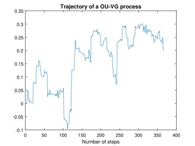
(a) OU-VG $X(0)=0$, $\theta=0.025$, $k=0.2$, $\nu=0.02$, $\sigma=0.3$.

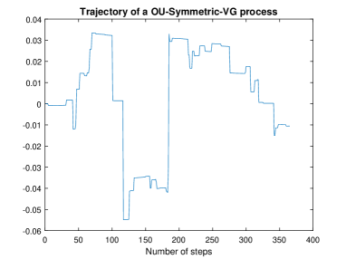
(b) OU-SVG with $X(0)=0$, $k=0.2162$, $\nu=0.256$, $\sigma=0.201$.

		$\bm{E}\left[{X(T)}\right]=0.0490$		$\bm{V}\left[{X(T)}\right]=0.0185$		$\bm{Skew}\left[{X(T)}\right]=0.529$		$\bm{Kurt}\left[{X(T)}\right]=4.689$
$T=1/5,\Delta t=1/5$
$N_{S}$	CPU	MC	error %	MC	error %	MC	error %	MC	error %
$2500$	$0.05$	$0.0475$	$3.14$	$0.0188$	$1.68$	$0.537$	$1.52$	$4.786$	$2.05$
$10000$	$0.20$	$0.0491$	$0.17$	$0.0182$	$1.57$	$0.502$	$5.08$	$4.637$	$1.12$
$40000$	$0.77$	$0.0489$	$0.31$	$0.0187$	$1.07$	$0.529$	$0.07$	$4.703$	$0.30$
$160000$	$3.06$	$0.0494$	$0.82$	$0.0186$	$0.48$	$0.535$	$1.17$	$4.666$	$0.49$
$640000$	$12.32$	$0.0489$	$0.19$	$0.0185$	$0.02$	$0.522$	$1.39$	$4.646$	$0.93$
$2560000$	$49.39$	$0.0491$	$0.18$	$0.0185$	$0.11$	$0.527$	$0.38$	$4.678$	$0.24$
		$\bm{E}\left[{X(T)}\right]=0.2266$		$\bm{V}\left[{X(T)}\right]=0.0793$		$\bm{Skew}\left[{X(T)}\right]=0.238$		$\bm{Kurt}\left[{X(T)}\right]=3.342$
$T=1,\Delta t=1/5$
$2500$	$0.28$	$0.2236$	$1.31$	$0.0786$	$0.97$	$0.214$	$9.81$	$3.220$	$3.67$
$10000$	$1.02$	$0.2270$	$0.18$	$0.0800$	$0.83$	$0.248$	$4.31$	$3.332$	$0.30$
$40000$	$4.02$	$0.2272$	$0.28$	$0.0802$	$1.15$	$0.236$	$0.70$	$3.315$	$0.83$
$160000$	$16.03$	$0.2268$	$0.09$	$0.0794$	$0.10$	$0.230$	$3.42$	$3.316$	$0.78$
$640000$	$64.46$	$0.2261$	$0.20$	$0.0793$	$0.02$	$0.239$	$0.55$	$3.341$	$0.03$
$2560000$	$258.51$	$0.2265$	$0.06$	$0.0793$	$0.10$	$0.238$	$0.30$	$3.338$	$0.12$

Table 1: CPU times in seconds and comparison among the true $\bm{E}\left[{X(T)}\right]$, $\bm{V}\left[{X(T)}\right]$, $\bm{Skew}\left[{X(T)}\right]$ and $\bm{Kurt}\left[{X(T)}\right]$ of a OU-VG process with $(k,\theta,\nu,\sigma,X(0))=(0.2,0.25,0.1,0.3,0)$ and their relative estimated values with $N_{S}$ MC scenarios.

	$T=1/5,\Delta t=1/5$					$T=1,\Delta t=1/5$
		$\bm{V}\left[{X(T)}\right]=0.0077$		$\bm{Kurt}\left[{X(T)}\right]=6.84$			$\bm{V}\left[{X(T)}\right]=0.0328$		$\bm{Kurt}\left[{X(T)}\right]=3.780$
$N_{S}$	CPU	MC	error %	MC	error %	CPU	MC	error %	MC	error %
$2500$	$0.04$	$0.0079$	$1.96$	$6.89$	$0.67$	$0.20$	$0.0303$	$7.69$	$3.341$	$11.61$
$10000$	$0.12$	$0.0075$	$2.73$	$6.66$	$2.62$	$0.64$	$0.0328$	$0.07$	$3.748$	$0.84$
$40000$	$0.53$	$0.0078$	$0.66$	$6.96$	$1.79$	$2.50$	$0.0327$	$0.29$	$3.853$	$1.94$
$160000$	$2.04$	$0.0077$	$0.73$	$6.91$	$1.03$	$10.16$	$0.0326$	$0.71$	$3.717$	$1.66$
$640000$	$8.06$	$0.0077$	$0.18$	$6.78$	$0.88$	$39.98$	$0.0327$	$0.38$	$3.793$	$0.35$
$2560000$	$32.10$	$0.0078$	$0.32$	$6.85$	$0.16$	$159.84$	$0.0328$	$0.04$	$3.778$	$0.05$

Table 2: CPU times in seconds and comparison among the true $\bm{V}\left[{X(T)}\right]$ and $\bm{Kurt}\left[{X(T)}\right]$ of a OU-Symmetric VG process with $(k,\nu,\sigma,X(0))=(0.2162,0.256,0.201,0)$ and their relative estimated values with $N_{S}$ MC scenarios

4 Financial Applications

Pricing derivative contracts or energy facilities is often accomplished using MC methods; for this purpose is therefore, necessary to rely on efficient and eventually, fast path-generation techniques. On the other hand, the day-ahead (also called spot) price of power or gas and in general of commodities exhibit mean-reversion, seasonality and spikes, this last feature is particularly difficult to be captured in a pure Gaussian world. Different approaches have been investigated in order to somehow extend the classical Gaussian framework introduced in Lucia and Schwarz [32] and Schwartz and Smith [40]. Among others, Cartea and Figueroa [12], Kjaer [28], Meyer-Brandis and P. Tankov [34] have studied mean-reverting jump-diffusions to model sudden spikes, whereas, Benth et al. [7] and Benth and A. Pircalabu [8] have considered different non-Gaussian OU processes in order to price power or wind derivative contracts. Recently, Cummins et al. [18, 19] have addresses the pricing of gas storages via FFT in a market driven by a OU-SVG process.

In the following subsections we illustrate the effectiveness of the algorithms presented in subsection 3.1 when applied to the pricing of Asian options and of gas storages using market models similar to those considered in Cummins et al. [18, 19]. Of course, MC methods are known to be sometimes slower than FFT and other techniques, nevertheless, they provide a view on the distribution of the potential cash-flows of derivative contracts giving a precious information to risk managers or to trading units. The calibration and in general, the parameter estimation of OU-VG processes is not the aim of the paper. However, as observed in Wolfe [42], discrete first-order autoregressive processes are embedded into continuous OU processes, therefore one could use the generalized method of moments (GMM) to derive Yule-Walker-like equations and estimate the model parameters from historical data.

4.1 Asian Options

In this section we assume that the spot price of a gas market is driven by the following $2$-factors process

$$S(t)=F(0,t)\,e^{h(t)+X_{1}(t)+X_{2}(t)}=F(0,t)\,e^{h(t)+H(t)}$$ (20)

where $h(t)$ is a deterministic function, $F(0,t)$ is the forward curve and $X_{1}(t)$ is a OU-VG process with parameters ($k,\theta_{1},\nu_{1},\sigma_{1}$). In contrast to Cummins et al. [19], we add a second independent VG process $X_{2}(t)$ with parameters $(\theta_{2},\nu_{2},\sigma_{2}$) to capture the long-term behavior. Using the risk-neutral arguments of the Lemma 3.1 in Hambly et al. [25], the deterministic function $h(t)$ consistent with forward curve is

$$h(t)=-\kappa_{H}(1,t).$$ (21)

where $\kappa_{H}(u,t)$ is the cumulant function of the process $H(t)$ at time $t$, then because of Equations (12) and (17)

$$h(t) = -\frac{1}{k\nu}\left(\DiLog{\frac{\mu_{p}}{\nu_{p}}}-\DiLog{\frac{\mu_{p}\,e^{-kt}}{\nu_{p}}}+\DiLog{-\frac{\mu_{n}}{\nu_{n}}}-\DiLog{-\frac{\mu_{n}\,e^{-kt}}{\nu_{n}}}\right)-$$ (22)

$$\frac{t}{\nu}\log\left(1-\theta\nu-\frac{\sigma^{2}\nu}{2}\right),$$

where $\mu_{p},\nu_{p},\mu_{n},\nu_{n}$ are relative to the parameters of $X_{1}(t)$.

Finally, we recall that the payoff at maturity $T$ of an Asian option with European style and strike price $K$ is

$$A(T)=\left(\sum_{i=1}^{d}\omega_{i}S(t_{i})-K\right)^{+}.$$

In our numerical experiments we assume an at-the-money Asian option $K=F(0,0)=15$ having one year maturity, $T=1$, with equal weights $\omega_{i}=1/d$ and with a flat forward curve. Although, as already mentioned, we do not focus on the parameters estimation, the values in Table 3(a) could be considered realistic because they are based on the estimations presented in Gardini et al. [21] for $X_{2}(t)$ and are similar to those shown in Cummins et al. [18] for $X_{1}(t)$; Figure 2(a) shows one sample price-path generated with Algorithm 1 using the market model of Equation (20).

Table 3: Asian option in a $2$-Factors market dynamics

Parameter	Value
$F(0,0)$	$15$
$K$	$15$
$T$	$1$
$d$	$360$
$\kappa_{1}$	$0.1859$
$\theta_{1}$	$0.05$
$\nu_{1}$	$0.4513$
$\sigma_{1}$	$0.203$
$\theta_{2}$	$0.1$
$\nu_{2}$	$0.2$
$\sigma_{2}$	$0.3$

(a) Parameters

$N_{S}$	CPU	price	stdev	error	%-error
$1000$	$7.59$	$1.219$	$2.24$	$0.071$	$5.82$%
$10000$	$74.87$	$1.229$	$2.34$	$0.023$	$1.90$%
$20000$	$149.03$	$1.227$	$2.26$	$0.016$	$1.30$%
$50000$	$386.10$	$1.231$	$2.26$	$0.010$	$0.82$%
$100000$	$743.03$	$1.236$	$2.27$	$0.0072$	$0.58$%

(b) Results

Figure 2: Price Trajectories

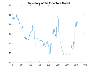
(a) $2$-factors Model

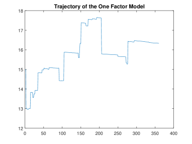
(b) One factor Model

Table 3(b) shows the estimated prices obtained by MC varying the number of simulations $N_{S}$, along with the overall computational times (CPU) in seconds. The columns stdev and error report the standard deviations of the MC estimator and the errors around the estimated option prices defined as the standard deviation divided by $\sqrt{N_{S}}$. The results illustrate that our simulation scheme is accurate indeed, the price of the option converges rapidly and the errors are very small; it seems that $10000$ simulations are good enough to have a reliable Asian option price. On the other hand, although here combined with the simulation of a standard VG process, the simulation of a OU-VG process is not extremely fast compared to the one of other generalized OU-processes (see for instance Cufaro Petroni and Sabino [16, 17]). Nevertheless, it provides additional information, such as quantiles of the price distribution, that can be employed to derive risk premia and support decision making and in particular, can give an insight whether the calibrated parameters imply realistic price trajectories.

4.2 Gas Storages

In contrast to the previous subsection, in the following we consider a one factor gas market similar to the model discussed in Cummins et al. [18]

$$S(t)=F(0,t)e^{h(t)+X(t)},$$ (23)

where $X(t)$ is OU-SVG with parameters $(k,\nu,\sigma)$ and once more, because of risk-neutral arguments

$$h(t)=-\frac{1}{2k\nu}\left(\text{Li}_{2}\left(\frac{\sigma^{2}\nu}{2}\right)-\text{Li}_{2}\left(\frac{\sigma^{2}\nu}{2}\,e^{-kt}\right)\right).$$ (24)

We then adopt this market dynamics for the pricing of a fast-churn gas storage. To this end, denote by $C(t)$ the volume of a gas storage at time $t$ with $C_{min}\leq C(t)\leq C_{max}$. The holder of such an energy asset is faced with a timing problem that consists in deciding when to inject, to withdraw or to do-nothing.

Denoting $J(t,x,c)$ the value of a gas storage at time $t$ given $S(t)=x$, $C(t)=c$, one can write:

$$J(t,x,c)=\sup_{u\in\mathcal{U}}\mathbb{E}\left[\int_{t}^{T}\phi_{u}\left(S(s)\right)ds+q\left(S(T),C(T)\right)\,\right|S(t)=x,C(t)=c\bigg{]},$$ (25)

where $\mathcal{U}$ denotes the set of the admissible strategies, $u(t)\in\{-1,0,1\}$ is the regime at time $t$ such that

$$\left\{\begin{array}[]{lcll}\phi_{-1}(S(t))&=&-S(t)-K_{in}a_{in},&\text{injection}\\ \phi_{0}(S(t))&=&-K_{N},&\text{do nothing}\\ \phi_{1}(S(t))&=&S(t)-K_{out}a_{w}&\text{withdrawal}\end{array}\right.,$$ (26)

$a_{in}$ and $a_{w}$ are the injection and withdrawal rates, $K_{in}$, $K_{out}$ and $K_{N}$, respectively, represent the costs of injection, do-nothing and withdrawal, and $q$ takes into account the possibility of final penalties. Based on the Bellman recurrence equation (see Bertsekas [9]), one can perform the following backward recursion for $i=1,\dots,d$:

$$J(t_{i},x,c)=\sup_{k\in\{-1,0,1\}}\left\{\phi_{k}S(t_{i})+\mathbb{E}\left[J\left(t_{i+1},S(t_{i+1}),\tilde{c}_{k}\right)|S(t_{i})=x,C(t_{i})=c\right]\right\},i=1,\dots,d,$$ (27)

where

$$\left\{\begin{array}[]{lll}\tilde{c}_{-1}&=&\min(c+a_{in},C_{max})\\ \tilde{c}_{0}&=&c\\ \tilde{c}_{1}&=&\min(c-a_{w},C_{min}).\\ \end{array}\right.$$ (28)

A standard approach to price gas storages is a modified version of the Least-Squares Monte Carlo (LSMC), introduced in Longstaff-Schwartz [31], detailed in Boogert and de Jong [11]. With this approach, the backward recursion is obtained by defining a finite volume grid of G steps for the admissible capacities $c$ of the plant and then apply the LSMC methodology to the continuation value per volume step. In alternative, one may solve the recursion by adapting the method proposed by Ben-Ameur et al. [6] or might use the quantization method as explained in Bardou et al. [1] or even FFT and Fourier techniques described for instance in Jaimungal and Surkov [26].

Finally, we consider a one-year fast-churn storage with the parameters shown in Table 4(a) such that $20$ days are required to fill or empty the storage. Our framework is similar to the one presented in Cummins et. al. [18] and we select the parameters of the OU-SVG shown therein. Once again, we assume a flat forward curve that does not change the validity of our experiment because we price a fast-churn storage whose extrinsic value is dominated by the short-term decisions rather than by the seasonality of the forward curve. In this case, Figure 2(b) shows one sample price-path generated with Algorithm 2 using the market model of Equation (23).

The columns of Table 4(b) have the same meaning of those presented in the analysis of the Asian option. In addition, the column CPU^∗ reports the computational times relative to the path simulation only, using Algorithm 2. Indeed, the computational cost of the standard LSMC method can be split into a path generation step and into a stochastic optimization step, with the computational cost of the latter one being independent on the price dynamics and being the dominant factor to the overall computational time (CPU in Table 4(b)). In this example, the CPU^∗’s are approximately, one forth of the overall time, and in particular, are almost a half of the overall time required to price an Asian option with the same number of simulations. Once again, the results show that our methodology is accurate and reasonably fast. However, although still acceptable, the CPU^∗’s are higher that those required to simulate other generalized OU processes. For instance, one of the reasons why Cummins et al. [18] investigated the use of OU-SVG was to reduce the number of model parameters compared to the mean-reverting jump-diffusion model discussed in Kjaer [28]. In this last case however, Cufaro Petroni and Sabino [16] have presented a fast simulation algorithm for mean-reverting jump-diffusion dynamics including the case of the mean-reverting equivalent of the Kou [29] model. These computational times are faster that those presented in this study because they almost completely cut off the time needed for the path simulation that therefore, becomes negligible compared to that of the optimization step.

It is worthwhile noticing that the performance of standard LSMC could be improved relying on the backward simulation of the price dynamics as explained in Pellegrino and Sabino [35] and Sabino [37]. This means that one has to design a backward simulation algorithm for the OU-VG process that will be the objective of a future research. The results of Table 4(b) show that one should rely on at least $N_{S}=10000$ sample paths to get an acceptable price. Of course, this also depends on the granularity of the volume grid: we have chosen $100$ equally-spaced steps. The computational performance of the LSMC based on Algorithm 2 is inferior to that of other numerical techniques such as FFT based approaches. Nevertheless, it has the advantage to be applicable to any payoff function, in contrast to FFT techniques that have to be adapted to each particular contract.

Table 4: Gas Storage in a $1$-Factors market dynamics

Parameter	Value
$F(0,0)$	$15$
$T$	$1$
$d$	$360$
$\kappa$	$0.2162$
$\nu$	$0.2560$
$\sigma$	$0.2021$
$C(0)$	$0$
$C(T)$	$0$
$a_{in}$	$1$
$a_{w}$	$1$
$C_{max}$	$20$

(a) Parameters

$N_{S}$	CPU	CPU∗	price	stdev	error	%-error
$1000$	$12.92$	$4.74$	$8.79$	$0.33$	$0.011$	$0.12$%
$10000$	$166.84$	$47.08$	$5.20$	$0.49$	$0.005$	$0.09$%
$20000$	$307.39$	$92.16$	$5.24$	$0.34$	$0.002$	$0.05$%
$50000$	$823.98$	$139.01$	$5.10$	$0.37$	$0.002$	$0.03$%
$100000$	$1557.09$	$465.41$	$5.13$	$0.36$	$0.001$	$0.02$%

(b) Storage Results

5 Conclusions

In this paper we have introduced a three-steps procedure to determine the law of the increment of generalized OU processes relying on the role of self-decomposability in the theory of such processes. Based on this machinery and the results of Qu et al. [36], we have developed efficient and accurate algorithms for the exact simulation of the OU-VG and OU-SVG processes discussed in Cummins et al. [18, 19] and Cufaro et al. [15]. The algorithms are accurate, efficient, and have been numerically tested, with the associated performance reported in detail. In addition, our three-steps procedure simplifies some of the proofs presented in the cited papers and could be employed to find simulation algorithms of other generalized OU processes that will the object of future inquires.

These results are instrumental to design algorithms to price derivative contracts in energy markets by MC simulation. To this end, we have considered the case of an Asian option in a market driven by the sum of a standard VG and a OU-VG process and the case of a fast-churn gas storage in a market driven by a OU-SVG process using the LSMC method of Boogert and de Jong [11]. Although, MC methods are slower than other numerical solutions, our algorithms give the possibility to compute the entire price distribution of derivative contracts. Although the parameters estimation is not the focus of our study, MC based techniques can also be a viable route to estimate the model parameters because the likelihood method is impracticable. Moreover, they can provide a graphical evidence that calibrated parameters correspond to realistic sample paths.

It is also worth noticing that all the algorithms that we have discussed are based on the sequential generation of processes. Therefore, a last topic deserving further investigation is the possibility to simulate OU-VG processes backward in time extending the results of Pellegrino and Sabino [35] and Sabino [37].

References

- [1] O. Bardou, S. Bouthemy, and G. Pagés. Optimal quantization for the pricing of swing options. Applied Mathematical Finance, 16(2):183–217, 2009.
- [2] O. E. Barndorff-Nielsen, J. L. Jensen, and M. Sørensen. Some Stationary Processes in Discrete and Continuous Time. Advances in Applied Probability, 30(4):989–1007, 1998.
- [3] O.E. Barndorff-Nielsen. Processes of Normal Inverse Gaussian Type. Finance and Stochastics, 2(1):41–68, 1998.
- [4] O.E. Barndorff-Nielsen and N. Shephard. Non-Gaussian Ornstein-Uhlenbeck-based Models and some of their Uses in Financial Economics. Journal of the Royal Statistical Society: Series B, 63(2):167–241, 2001.
- [5] O.E. Barndorff-Nielsen and N. Shephard. Integrated OU Processes and non-Gaussian OU-based Stochastic Volatility Models. Scandinavian Journal of Statistics, 30(30):277–295, 2003.
- [6] H. Ben-Ameur, M. Breton, L. Karoui, and P. L’Ecuyer. A Dynamic Programming Approach for Pricing Options Embedded in Bonds. Journal of Economic Dynamics and Control, 31(7):2212–2233, July 2007.
- [7] F.E. Benth, J. Kallsen, and T. Meyer-Brandis. A non-gaussian ornstein-uhlenbeck process for electricity spot price modeling and derivatives pricing. Applied Mathematical Finance, 14(2):153–169, 2007.
- [8] F.E. Benth and A. Pircalabu. A non-Gaussian Ornstein-Uhlenbeck Model for Pricing Wind Power Futures. Applied Mathematical Finance, 25(1), 2018.
- [9] D. P. Bertsekas. Dynamic Programming and Optimal Control, Volume I. Athena Scientific, Belmont, Mass., third edition, 2005.
- [10] M.L. Bianchi, S.T. Rachev, and F.J. Fabozzi. Tempered Stable Ornstein-Uhlenbeck Processes: A Practical View. Communications in Statistics - Simulation and Computation, 46(1):423–445, 2017.
- [11] A. Boogert and C. de Jong. Gas Storage Valuation Using a Monte Carlo Method. Journal of Derivatives, 15:81–91, 2008.
- [12] A. Cartea and M. Figueroa. Pricing in Electricity Markets: a Mean Reverting Jump Diffusion Model with Seasonality. Applied Mathematical Finance, No. 4, December 2005, 12(4):313–335, 2005.
- [13] R. Cont and P. Tankov. Financial Modelling with Jump Processes. Chapman and Hall, 2004.
- [14] N. Cufaro Petroni. Self-decomposability and Self-similarity: a Concise Primer. Physica A, Statistical Mechanics and its Applications, 387(7-9):1875–1894, 2008.
- [15] N. Cufaro Petroni, S. De Martino, S. De Siena, and F. Illuminati. Stationary Distribution of non-Gaussian Ornstein-Uhlenbeck Processes for Beam Halos. In Proceedings of the Conference CYCLOTRONS 07, page 424, 2008. Giardini Naxos, Italy, 1-5 October 2007; INFN Catania.
- [16] N. Cufaro Petroni and P. Sabino. Fast Pricing of Energy Derivatives with Mean-reverting Jump-diffusion Processes. Available at: https://arxiv.org/abs/1908.03137.
- [17] N. Cufaro Petroni and P. Sabino. Gamma Related Ornstein–Uhlenbeck Processes and their Simulation. available at: https://arxiv.org/abs/2003.08810.
- [18] M. Cummins, G. Kiely, and B. Murphy. Gas Storage Valuation under Lévy Processes using Fast Fourier Transform. Journal of Energy Markets, 4:43–86, 2017.
- [19] M. Cummins, G. Kiely, and B. Murphy. Gas Storage Valuation under Multifactor Lévy Processes. Journal of Banking and Finance, 95:167–184, 2018.
- [20] L. Devroye. Non-Uniform Random Variate Generation. Springer-Verlag, 1986.
- [21] M. Gardini, P. Sabino, and E. Sasso. Correlating Lévy Processes with Self-decomposability: Applications to Energy Markets. Available at: https://arxiv.org/abs/2004.04048.
- [22] D. P. Gaver and P. A. W. Lewis. First-order Autoregressive Gamma Sequences and Point Processes. Advances in Applied Probability, 12(3):727–745, 1980.
- [23] I. S. Gradshteyn and I. M. Ryzhik. Table of Integrals, Series, and Products. Elsevier/Academic Press, Amsterdam, seventh edition, 2007.
- [24] B. Grigelionis. On the Self-Decomposability of Euler’s Gamma Function. Lithuanian Mathematical Journal, 43(3):295–305, 2003.
- [25] B. Hambly, S. Howison, and T. Kluge. Information-Based Models for Finance and Insurance. Quantitative Finance, 9(8):937–949, 2009.
- [26] S. Jaimungal and V. Surkov. Lévy Based Cross-commodity Models and Derivative Valuation. SIAM Journal of Financial Mathematics, 2:464–487, 2011.
- [27] M. Joshi. The Concept and Practice of Mathematical Finance. Cambridge University Press, 2003.
- [28] M. Kjaer. Pricing of Swing Options in a Mean Reverting Model with Jumps. Applied Mathematical Finance, 15(5-6):479–502, 2008.
- [29] S. G. Kou. A Jump-Diffusion Model for Option Pricing. Manage. Sci., 48(8):1086–1101, August 2002.
- [30] A.J Lawrance. Some Autoregressive Models for Point Processes. In P. Bartfai and J. Tomko, editors, Point Processes and Queueing Problems (Colloquia Mathematica Societatis János Bolyai 24), volume 24, pages 257–275. North Holland, 1980.
- [31] F. A. Longstaff and E.S. Schwartz. Valuing American Options by Simulation: a Simple Least-Squares Approach. Review of Financial Studies, 14(1):113–147, 2001.
- [32] J.J. Lucia and E.S. Schwartz. Electricity Prices and Power Derivatives: Evidence from the Nordic Power Exchange. Review of Derivatives Research, 5(1):5–50, 2002.
- [33] D. B. Madan and E. Seneta. The Variance Gamma (V.G.) Model for Share Market Returns. The Journal of Business, 63(4):511–24, 1990.
- [34] T. Meyer-Brandis and P. Tankov. Multi-factor Jump-diffusion Models of Electricity Prices. International Journal of Theoretical and Applied Finance, 11(5):503–528, 2008.
- [35] T. Pellegrino and P. Sabino. Enhancing Least Squares Monte Carlo with Diffusion Bridges: an Application to Energy Facilities. Quantitative Finance, 15(5):761–772, 2015.
- [36] Y. Qu, A. Dassios, and H. Zhao. Exact Simulation of Gamma-driven Ornstein–Uhlenbeck Processes with Finite and Infinite Activity Jumps. Journal of the Operational Research Society, 0(0):1–14, 2019.
- [37] P. Sabino. Forward or Backward Simulations? A Comparative Study. Quantitative Finance, 2020. Forthcoming.
- [38] K. Sato. Lévy Processes and Infinitely Divisible Distributions. Cambridge U.P., Cambridge, 1999.
- [39] W. Schoutens. Lévy Processes in Finance: Pricing Financial Derivatives. John Wiley and Sons Inc, 2003.
- [40] P. Schwartz and J.E. Smith. Short-term Variations and Long-term Dynamics in Commodity Prices. Management Science, 46(7):893–911, 2000.
- [41] E. Taufer and N. Leonenko. Simulation of Lévy-driven Ornstein–Uhlenbeck Processes with Given Marginal Distribution. Computational Statistics & Data Analysis, 53(6):2427 – 2437, 2009. The Fourth Special Issue on Computational Econometrics.
- [42] S.J. Wolfe. On a Continuous Analogue of the Stochastic Difference Equation . Stochastic Processes and their Applications, 12(3):301 – 312, 1982.