∎
22email: gangl(at)math.tugraz.at 33institutetext: K. Sturm44institutetext: TU Wien, Wiedner Hauptstr. 8-10, 1040 Vienna
44email: kevin.sturm(at)tuwien.ac.at 55institutetext: M. Neunteufel66institutetext: TU Wien, Wiedner Hauptstr. 8-10, 1040 Vienna
66email: michael.neunteufel(at)tuwien.ac.at 77institutetext: J. Schöberl88institutetext: TU Wien, Wiedner Hauptstr. 8-10, 1040 Vienna
88email: joachim.schoeberl(at)tuwien.ac.at
Fully and Semi-Automated Shape Differentiation in NGSolve
Abstract
In this paper we present a framework for automated shape differentiation in the finite element software NGSolve. Our approach combines the mathematical Lagrangian approach for differentiating PDE constrained shape functions with the automated differentiation capabilities of NGSolve. The user can decide which degree of automatisation is required, thus allowing for either a more custom-like or black-box-like behaviour of the software. We discuss the automatic generation of first and second order shape derivatives for unconstrained model problems as well as for more realistic problems that are constrained by different types of partial differential equations. We consider linear as well as nonlinear problems and also problems which are posed on surfaces. In numerical experiments we verify the accuracy of the computed derivatives via a Taylor test. Finally we present first and second order shape optimisation algorithms and illustrate them for several numerical optimisation examples ranging from nonlinear elasticity to Maxwell’s equations.
Keywords:
shape optimisation, shape derivative, automated differentiation, shape Newton method1 Introduction
Numerical simulation and shape optimisation tools to solve the problems have become an integral part in the design process of many products. Starting out from an initial design, non-parametric shape optimisation techniques based on first and second order shape derivatives can assist in finding shapes of a product which are optimal with respect to a given objective function. Examples include the optimal design of aircrafts a_SCILSCGA_2013 ; a_SCILSCGA_2011a , optimal inductor design a_HOSO_2003a , optimisation of microlenses a_PASAHIHA_2015a , the optimal design of electric motors GLLMS2015 , applications to mechanical engineering AllaireJouveToader2004 ; a_LA_2018a , multiphysics problems Feppon2019Sep or electrical impedance tomography (EIT) in medical sciences to name only a few a_HILA_2008a .
Shape optimisation algorithms are based on the concept of shape derivatives. Let denote the set of all subsets of . Further let be a set of admissible shapes and be a shape function. Given an admissible shape and a sufficiently smooth vector field , we define the perturbed domain for a small perturbation parameter . The shape derivative is defined as
| (1) |
Remark 1
We remark that a frequently used definition of shape differentiability is to require the mapping being Fréchet differentiable in ; see b_AL_2007a ; b_HEPI_2005a ; a_MUSI_1976a . This stronger notion of differentiability implies that the limit defined in (1) exists.
In most practically relevant applications, the objective functional depends on the shape of a (sub-)domain via the solution to a partial differential equation (PDE). Thus, one is facing a problem of PDE-constrained shape optimisation of the form
| (2) |
Here, the second line represents the constraining boundary value problem posed on a Hilbert space , which we assume to be uniquely solvable for all admissible . Denoting the unique solution for a given by , we introduce the notation for the reduced functional
In order to be able to apply a shape optimisation algorithm to a given problem of this kind, the shape derivative (1) has to be computed, see the standard literature DZ2 ; SZ or a_ST_2015a for an overview of different approaches. In the following we focus on computing the so-called volume form of the shape derivative which in a finite element context is known to give a better approximation compared to the boundary form; see MR3348199 ; MR2642680 .
The convergence of shape optimisation algorithms can be speeded up by using second order shape derivatives. Given two sufficiently smooth vector fields , and an admissible shape , let be the perturbed domain. Then, the second order shape derivative is defined as
| (3) |
Second order information in Newton-type algorithms has been explored in the articles a_NORO_2002a ; a_ALCAVI_2016a ; a_PAST_2019a ; a_EPHASC_2007a ; a_VSC_2014a . Since the computation of second order shape derivatives is more involved and error prone, several authors have employed automatic differentiation (AD) tools, see e.g. a_SC_2018a and a_HAMIPAWE_2019a for two approaches based on the Unified Form Language (UFL) a_ALMALOOLROWE_2014a . In a_HAMIPAWE_2019a , the authors present a fully automated shape differentiation software which uses the transformation properties on the finite element level. In a_SC_2018a (see also the earlier work a_SC_2014a ) the automated derivatives are computed using UFL. The strategies of a_HAMIPAWE_2019a and a_SC_2018a differ in that, for the latter, the software computes an unsymmetric shape Hessian since it involves the term . Optionally the software allows to make the shape Hessian symmetric by requiring . We will discuss the subtle difference and the relation between the two possible ways of defining shape Hessians in Remark 3 of Section 3.2. Let us also mention a_DOMISEPU_2020a where automated shape derivatives for transient PDEs in FEniCS and Firedrake are presented.
In this paper we present an alternative framework for AD of PDE constrained problems of type (2). There exist several approaches for the rigorous derivation of the shape derivative of PDE-constrained shape functionals, see c_ST_2015a for an overview. The main idea, however, is always similar. After transforming the perturbed setting back to the original domain, shape differentiation in the direction of a given vector field reduces to the differentiation with respect to the scalar parameter which now enters via the corresponding transformation and its gradient. It is shown in a_ST_2015a that the shape derivative for a nonlinear PDE-constrained shape optimisation problem can be computed as the derivative of the Lagrangian with respect to the perturbation parameter. We will illustrate this systematic procedure for a number of different applications and utilise symbolic differentiation provided by the finite element software package NGSolve Schoeberl2014 to obtain the shape derivative for different classes of PDE-constrained optimisation problems. NGSolve allows for the fast and efficient numerical solution of a large number of different boundary value problems. The aim of this paper is to extend NGSolve by the possibility of semi-automatic and fully automatic shape differentiation and optimisation.
Distinctly from previous approaches we cover the following two points:
-
•
a fully automated setting requiring as input the weak formulation of the constraint and the cost function,
-
•
a semi-automated setting which offers a highly customisable user interface, but requires mathematical background knowledge.
Structure of the paper.
In Section 2 we give a brief introduction on how to solve a PDE in NGSolve and present its built-in auto-differentiation capabilities. The introduced syntax will also lay the foundation for the following sections. In Section 3 we present a first unconstrained shape optimisation problem and show how to solve it in NGSolve. For this purpose we show how to compute the first and second order shape derivative in a semi-automated way. Section 4 extends the preceding section by incorporating a PDE constraint. The strategy is illustrated by means of a simple Poisson equation. We also show how to treat the computation of shape derivatives when the PDE is defined on surfaces. While the semi-automated shape differentiation presented in Sections 3 and 4 requires mathematical background knowledge, in Section 5 we show how the shape derivatives can be computed in a fully automated fashion. In the last section of the paper we verify the computed formulas by a Taylor test, discuss optimisation algorithms and present several numerical optimisation examples including nonlinear elasticity, Maxwell’s equations and Helmholtz’s equation.
2 A brief introduction to NGSolve
In this section, we give a brief overview of the main concepts of the finite element software NGSolve Schoeberl2014 . We first describe the main principles for numerically solving boundary value problems in NGSolve before focusing on its built-in automatic differentiation capabilities. In the subsequent sections of this paper, these ingredients will be combined to implement the shape derivative of unconstrained and PDE-constrained shape optimisation problems in an automated way.
2.1 Solving PDEs with finite elements in NGSolve
In this section, we illustrate the syntax of NGSolve using the python programming language for the Poisson equation with homogeneous Dirichlet conditions as a model problem. We refer the reader to the online documentation
https://ngsolve.org/docu/latest/
for a more detailed description of the many features of this package.
Given a domain and a right hand side , we consider the model problem to find satisfying
The weak form of the model problem reads
| (4) |
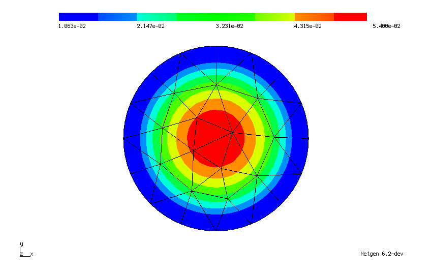
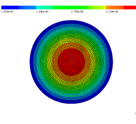
We consider a ball of radius in two space dimensions centered at the point , i.e. , and the right hand side is defined by . We will go through the steps for numerically solving this problem by the finite element method.
We begin by importing the necessary functionalities and setting up a finite element mesh.
The first line imports all modules from the package NGSolve. The second line includes the SplineGeometry function which enables us to define a mesh via a geometric description, in our case a circle centered at of radius . Finally the mesh is generated in line 7 and in line 8 we specify that we want to use a curved finite element mesh for a more accurate approximation of the geometry. For that purpose, a projection-based interpolation procedure is used, see e.g. demk04 .
Next in line 1 we define an conforming finite element space of polynomial degree and include Dirichlet boundary conditions on the boundary of the domain (referenced by the string ‘‘circle’’ that we assigned in line 5). On this space we define a trial function u in line 3 and a test function w in line 4. These are purely symbolic objects which are used to define boundary value problems in weak form.
For a more compact presentation later on, we define a coefficient function X which combines the three spatial components:
Now, the left and right hand sides of problem (4) can be conveniently defined as a bilinear or linear form, respectively, on the finite element space fes by the following lines.
We assemble the system matrix coming from the bilinear form a and the load vector coming from L and solve the corresponding system of linear equations.
Here, gfu is defined as a GridFunction over the finite element space fes. A GridFunction object is used to save the results by containing the corresponding finite element coefficient vectors. Further, it can evaluate the stored finite element solution at a given mesh point. The Dirichlet conditions are incorporated into the direct solution of the linear system and the numerical solution is drawn in the graphical user interface. The numerical solution is depicted in Figure 1.
2.2 Automatic Differentiation in NGSolve
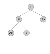
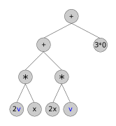
In NGSolve, symbolic expressions are stored in expression trees, see Figure 2 for an example. It is possible to differentiate an expression expr with respect to a variable var appearing in expr into a direction dir by the command
expr.Diff(var, dir).
Mathematically this line corresponds to the directional derivative of g:=expr at in direction , that is,
| (5) |
When calling the Diff command for expr, the expression tree of expr is gone through node by node, and for each node the corresponding differentiation rules such as product rule or chain rule are applied. When a node represents the variable with respect to which the differentiation is carried out, it is replaced by the direction dir of differentiation.
Figure 2 shows the differentiation of the expression expr= 2x*x+3y with respect to x into the direction given by v:
The output of print(expr) reads {verbnobox}[] coef binary operation ’+’, real coef binary operation ’*’, real coef scale 2, real coef coordinate x, real coef coordinate x, real coef scale 3, real coef coordinate y, real which translates to and corresponds to the expression tree depicted in Figure 2(a). The output of print(dexpr) reads {verbnobox}[] coef binary operation ’+’, real coef binary operation ’+’, real coef binary operation ’*’, real coef scale 2, real coef N5ngfem28ParameterCoefficientFunctionE, real coef coordinate x, real coef binary operation ’*’, real coef scale 2, real coef coordinate x, real coef N5ngfem28ParameterCoefficientFunctionE, real coef scale 3, real coef 0, real which translates to and corresponds to the expression tree depicted in Figure 2(b). The coefficient
| N5ngfem28ParameterCoefficientFunctionE |
appearing therein is the C++ internal class name of the Python object Parameter.
 |
 |
| (a) | (b) |
NGSolve trial and test functions are purely symbolic objects used for defining bilinear and linear forms. Therefore, they do not depend on the spatial variables , , as can be seen by differentiating them. NGSolve GridFunctions on the other hand represent functions in the finite element space. However, also for these objects, the space dependency is omitted when performing symbolic differentiation. The code segments
will give the following output: {verbnobox}[] Diff u w.r.t. x: ConstantCF, val = 0 Diff w w.r.t. x: ConstantCF, val = 0 Diff gf w.r.t. x: ConstantCF, val = 0 Here, the GridFunction.Set method takes a CoefficientFunction object and performs a (local) best-approximation into the underlying finite element space with respect to its natural norm and stores the resulting coefficient vector.
3 Semi-automatic shape differentiation without constraints
We will illustrate the steps to be taken in order to obtain the shape derivative of a shape function in a semi-automatic way for a simple shape optimisation problem. For bounded and open and a continuously differentiable function , we consider the shape differentiation of the shape function
| (6) |
Clearly the minimiser of over all measurable sets in is given by . We also refer to ubt_epub3251 for the computations of first and second order variations of functions of type (6) where is a submanifold of .
3.1 First order shape derivative
Henceforth we denote by the space of bounded and Lipschitz continuous vector fields . In view of Rademachers’ theorem (b_EV_2010a, , Thm.6, p.296) the space corresponds to the Sobolev space .
Given a vector field , we define the transformation
Definition 1
The first order shape derivative of a shape function at in direction is defined by
| (7) |
3.1.1 Shape differentiation of unconstrained volume integrals
Using the transformation and the notation for the Jacobian of the transformation , we get for as in (6),
| (8) |
Now let us explain how to compute the shape derivative of . Denoting
| (9) |
the chain rule gives (formally)
| (10) |
Using that and , we get for the shape derivative
This is the form we use for defining the first order shape derivative in NGSolve. Note that a Lipschitz vector field is differentiable almost everywhere and hence is defined almost everywhere and bounded.
Given the function with , and , we implement the transformed cost function (8) as follows:
Here, we introduce the symbol F and assign to it the value of the identity matrix in line 15. This allows us to differentiate with respect to F. Then we define the function of (9) in line 16. The shape derivative is a bounded linear functional on a space of vector fields. We introduce a vector-valued finite element space VEC and define the object representing the shape derivative dJOmega_f as a linear functional on VEC. In line 25, we differentiate with respect to the spatial variables in the direction given by V. Note that X is the coefficient function we introduced in line 8. In line 26, we deal with the differentiation with respect to F.
Remark 2
Defining and using , it holds
Therefore, we obtain for the first order shape derivative the well-known formula
| (11) |
Finally if is smooth enough (for instance ), it follows by integration by parts in (11) that the shape derivative is given by
| (12) |
where denotes the outward pointing normal along .
3.1.2 Shape differentiation of unconstrained boundary integrals
For and as in the previous section we consider
| (13) |
Then we get
| (14) | ||||
| (15) |
see e.g. (SZ, , Prop. 2.47), with the outer unit normal vector and denoting the Euclidean norm. It is shown in (SZ, , Prop. 2.50) that the shape derivative of (13) is given by
Again, we can compute the shape derivative in NGSolve as the total derivative of expression (15) with respect to the parameter . In NGSolve, the only difference lies in the necessity to use the trace of the gradient of a test vector field V.
Note that the trace operator for gradients on the boundary is obligatory in NGSolve, whereas for direct evaluation of trial and test functions itself it is optional.
3.2 Second order shape derivatives
For second order shape derivatives, we consider perturbations of the form
for and define .
Definition 2
The second order shape derivative of a shape function at in direction is defined by
| (16) |
Remark 3
We remark that if is smooth enough, the second order derivative as defined in (16) is symmetric by definition:
| (17) |
We stress that this derivative is not the same as the shape derivative obtained by repeated shape differentiation, that is, it does not coincide with (see, e.g., (b_DEZO_2011a, , Chap. 9, Sec. 6))
| (18) |
which is in general asymmetric.
The derivative defined in (18) is only symmetric if since it holds
| (19) |
see also the early work of Simon Simon1989 on this topic. However, in NGSolve, when repeating the shape differentiation procedure introduced in Section 3.1, we compute directly the second order shape derivative as defined in (16). Here, we exploit the fact that trial functions are independent of the spatial coordinates, see also Section 2.2 and the example below.
Let us now exemplify the computation of the second order shape derivative for the shape function defined in (6). Similarly to the computations of the first derivative, we use the notation . Then we get
Again, using the notation
we get
Using that and , we get further
| (20) |
Formula (20) is used for the automatic derivation of the second order shape derivative in NGSolve. Using , and , , we get
| (21) |
Remark 4
We remark that the formula (3.2) can be evaluated explicitly and reads
Formula (3.2) can be implemented in NGSolve as follows:
Notice that since W is a trial function it is not affected by the differentiation with respect to X, see Section 2.2. Therefore, the terms coming from differentiating W with respect to the spatial coordinates X into the direction of V disappear and thus, although code lines 29–30 look like the “derivative of the derivative”, we actually compute formula (16) and not (18).
In the same fashion, second order derivatives of boundary integrals of the form (13) can be computed.
Again note that the trace operator is necessary when dealing with gradients on the boundary.
4 Semi-automatic shape differentiation with PDE constraints
In this section, we describe the automatic computation of the shape derivative for the following type of equality constrained shape optimisation problems:
| (22) |
subject to solves
| (23) |
where with represents an abstract PDE constraint with being the union of Banach spaces and a set of admissible shapes. For any given we assume the PDE constraint (23) to admit a unique solution which we denote by . Moreover, let denote the reduced cost functional. By introducing a Lagrangian function, we can henceforth deal with an unconstrained shape function rather than a shape function and a PDE constraint. We introduce the Lagrangian
| (24) |
Now an initial shape is perturbed by a family of transformations , resulting in a new shape . Transforming back to the initial shape leads to the Lagrangian:
| (25) |
where is a bijective mapping. Here the transformation depends on the differential operator involved. For instance
-
•
if , then ,
-
•
if , then ,
-
•
if , then .
Intuitively the transformations are chosen in such a way that the transformed function still belongs to the same space, but on a different domain. For the above three examples this essentially requires to check how the differential operators , curl and div transform under the change of variables , respectively. In fact one can check that
where , see also (Monk2003, , Section 3.9). The transformation rules are precisely given by the respective . We also note that for smooth functions this can be checked by direct computation.
Now the shape differentiability of (22)–(23) is reduced to proving that (see c_ST_2015a )
| (26) |
where and solves and is the solution to the adjoint equation
| (27) |
We stress that the choice of as the solution of the adjoint equation is important in order for the second equality in (26) to hold. The verification of this equality depends on the specific PDE under consideration and can be accomplished by different methods. We refer the reader to c_ST_2015a for an overview and remark that (26) holds for a large class of nonlinear PDE constrained shape optimisation problems; see a_ST_2015a .
The rest of this section is organised as follows: We introduce a model problem, which is the minimisation of a tracking-type cost functional subject to Poisson’s equation in Section 4.1. We illustrate how the first and second order shape derivative for this PDE-constrained model problem can be obtained in NGSolve in Sections 4.2 and 4.3. Finally, we also briefly discuss the extension to partial differentiation equations on surfaces.
4.1 PDE-constrained model problem
We will illustrate the derivation of the first and second order shape derivative for the minimisation of a tracking-type cost functional subject to Poisson’s equation on the unknown domain . Let or , and be a set of admissible shapes. Here, denotes the power set of all subsets of . We consider the problem
| (28a) | |||
| subject to solves | |||
| (28b) | |||
for all . The Lagrangian is given by
| (29) |
Given an admissible shape , a vector field and small, let be the perturbed domain. Therefore the parametrised Lagrangian is given by
| (30) |
Changing variables yields
| (31) | ||||
where and . Here we also transformed the gradient according to for . Recall that, for a given , denotes the corresponding unique solution to (28b) and the reduced cost functional, . Let be the solution of the perturbed state equation brought back to the original domain , that is, is the unique solution to
| (32) |
Note that, for defined by (32), it holds for all and therefore also for all .
It can easily be shown that (26) holds and thus the shape derivative in the direction of a vector field is given by
where denotes the adjoint state and is defined as the unique solution to
| (33) |
or explicitly
| (34) |
4.2 First order shape derivative
By the discussion above, the first order shape derivative is given by with defined in (31) and and the unique solutions to the boundary value problems (28b) and (34), respectively.
Writing we obtain in analogy to the unconstrained problem
We can compute explicitly
| (35) | ||||
| (36) |
Now we are in a position to compute the first order shape derivative for the PDE-constrained shape optimisation problem (28) in NGSolve. After solving the state equation as shown in Section 2.1, the adjoint equation can be solved as follows.
We can now define the Lagrangian (31) such that the shape derivative can be obtained by the same procedure as in the unconstrained setting. Note that lines 29–30 coincide with lines 25–26.
4.3 Second order shape derivative
Let us introduce the notation
| (37) | ||||
| (38) |
and
| (39) |
where and . We observe that
| (40) |
with being the solution to
| (41) | ||||
| (42) |
for . In case we write and and similarly for we write and . Therefore, consecutive differentiation of (40) first with respect to at zero and then with respect to at zero yields
| (43) |
where solves the material derivative equation
| (44) |
for all or, equivalently
| (45) |
for all . Note that (45) is obtained by differentiating (41) with respect to and setting . Similarly the function solves the material derivative equation obtained by differentiating (42) with respect to for ,
| (46) |
for all . The introduction of the adjoint variable is analogous to the computation of the first order shape derivative. However in contrast to the first order derivative the evaluation of requires the computation of the material derivatives and .
Formally (44) and (46) can be written as an operator equation with ,
| (47) |
So to evaluate the second derivative (43) in some direction we have to solve the system (47).
This is realised in NGSolve by setting up a combined finite element space which we denote by X2. We define trial and test functions as well as grid functions representing the deformation vector fields and , which we initialise with some functions.
We define a 22 block bilinear form as well as a 21 block linear form which will represent the left and right hand sides of (47), respectively. The operator equation in (47) can be conveniently defined by differentiating the Lagrangian with respect to the corresponding variables.
We can solve this combined system for and and access and visualise the two components in the following way:
In order to obtain the second order shape derivative in the direction given by , it remains to evaluate the term (43). We define the three terms of (43) as bilinear forms, assemble them and perform vector-matrix-vector multiplications:
4.4 PDEs on surfaces
The automated shape differentiation is not restricted to partial differential equations on domains , but is readily extended to surface PDEs. We consider a two dimensional closed surface and denote by the normal field along . Let be given and define
| (48) |
where solves the surface equation
| (49) |
where denotes the tangential gradient of ; see (b_DEZO_2011a, , p.493, Def.5.1). We assume that the function is given. The Lagrangian is given by
As in the previous section we fix an admissible shape and let be a small perturbation of by means of a vector field for small. The parametrised Lagrangian is given by
| (50) |
Define the density . Changing variables and using
| (51) |
yields
| (52) |
where and .
Writing we obtain in analogy to the domain case
| (53) |
We can compute explicitly
| (54) | ||||
| (55) |
where denotes the tangential Jacobian of defined by for , and the tangential divergence, which is defined as the trace of the tangential Jacobian; see (b_DEZO_2011a, , p.495).
The implementation is analogous to the previous sections. We will only illustrate first order derivatives here. We first define the geometry of the unit sphere, create a surface mesh and define a finite element space on the surface mesh:
Next we define the transformed cost function and partial differential equation needed for setting up the Lagrangian (52). Here, we again make use of a symbolic object F to which we assign the identity matrix. We define the tangential determinant and the matrix defined in (51) as functions of the deformation gradient .
Now we can define the bilinear form and solve the state equation. Here, the right hand side of the equation is included in the bilinear form and the boundary value problem – although linear – is solved by Newton’s method (which terminates after only one iteration) for convenience.
Using Newton’s method for solving the linear boundary value problem allows us to define both the left and right hand side of the PDE using only one BilinearForm a (which, strictly speaking, is not bilinear any more). This way, we can reuse Equation_surf as defined in lines 74–75 to define the boundary value problem in line 71.
The adjoint equation is solved as usual:
The shape derivative is obtained as in the case of PDEs posed on volumes by the evaluation of (53):
5 Fully automated shape differentiation
In the previous sections we used the automatic differentiation capabilities of NGSolve to alleviate the shape differentiation procedure. However, so far we still had to include some knowledge about the problems at hand. So far, it was necessary to define the objective function or Lagrangian in the correct way, accounting for the correct transformation rules between perturbed and unperturbed domain. In this section, we will show that also this step can be automated since all necessary information is already included in the functional setting. The fully automated shape differentiation is incorporated by the command
DiffShape(...).
In particular, in the fully automated setting it is enough to set up the cost function or Lagrangian for the unperturbed setting. For a shape function of the type (6) we can define the shape derivative of the cost function in the following way:
Note that there is no term of the form Det(F) showing up in line 85. Here, the transformation of the domain is taken care of automatically. It can be checked that this really gives the same result as dJOmega_f defined in lines 25–26.
The above code gives the output {verbnobox}[] —dJOmega_f - dJOmega_f_0— = 1.571008573810619e-17 which confirms our claim. The same holds true for second order shape derivatives. The lines 29–30 can be replaced by a repeated call of DiffShape(...):
Again, it can be verified that d2JOmega_f_0 coincides with the previously defined quantity d2JOmega_f. Note that slightly different results may occur due to different integration rules used. This can be cured by enforcing an integration rule of higher order for G_f, i.e. by replacing the symbol dx in the definition of G_f with dx(bonus_intorder=2).
In the more general setting of PDE-constrained shape optimisation, the procedure is very similar. Here the idea exploited in the implementation of the command DiffShape(...) is to just differentiate the general expression (25) with respect to the parameter . The transformations appearing in (25), which depend on the functional setting of the PDE, are identified automatically from the finite element space from which the corresponding functions originate. The shape derivative of lines 29–30 can be obtained by the following code.
Here, gfu and gfp represent the solutions to the state and adjoint equation, respectively, and must have been computed previously. The bilinear form shapeHess11 used in Section 4.3 (see lines 47–48) can be obtained similarly:
The same holds true for boundary integrals
and surface PDEs
as well as their respective second order derivatives.
Remark 5
We remark that the fully automated differentiation using DiffShape(...) should be seen to complement the semi-automated shape differentiation techniques introduced in Sections 3 and 4 rather than to replace them. Using the semi-automated differentiation, the user has the possibility to, on the one hand, keep control over the involved terms, and on the other hand also to adjust the shape differentiation to their custom problems which may be non-standard. As an example where the semi-automated differentiation may be beneficial compared to the fully automated differentiation we mention the case of time-dependent PDE constraints considered in a space-time setting when a shape deformation is only desired in the spatial coordinates, see Section 7.8. Of course, when one is interested in the shape derivative for a more standard problem, the fully automated way appears to be more convenient and less error prone.
Remark 6
We have seen that the command DiffShape(…) allows to compute the shape derivative of unconstrained shape optimisation problems in a fully automated way without specifying any transformation rules, see line 87. For the practically more relevant case of PDE-constrained shape optimisation problems, the state and adjoint equations have to be solved beforehand also in the fully automated context using DiffShape(…). We remark that this can be easily achieved by defining a custom function solvePDE() as it is done for the case of a linear PDE in lines 99–106. Since the purpose of this paper is to illustrate a convenient way of computing shape derivatives and performing shape optimisation rather than to provide a tool for black-box optimisation, this step is left to the user and is not automated, leaving more freedom in the choice of, e.g., solvers for the arising linear systems.
6 Optimisation algorithms
In this section we discuss how to use optimisation algorithms in conjunction with the automated shape differentiation explained in the previous sections. The starting point of our discussion is a fixed initial shape . Then we consider the mapping
| (56) |
defined on a suitable space of vector fields . Since the mapping is defined on an open subset of the Banach space we can employ standard algorithms to minimise over . The only constraint we must impose is that remains invertible, which can be difficult in practice. In view of for and small, we find by differentiating with respect to at , that
| (57) |
for and invertible.
6.1 Gradient computation
The gradient of in a Hilbert space is defined by
| (58) |
Typical choices for are
| (59) | ||||
| (60) | ||||
| (61) |
where , and
| (62) |
The last choice, which is restricted to the spatial dimension , corresponds to a penalised Cauchy-Riemann gradient and results in a gradient which is approximately conformal and hence preserves good mesh quality. We refer to a_IGSTWE_2018a for a detailed description. We also refer to a_GO_2006a ; a_BU_2002a and a_ALDAJO_2020a for the use of different inner products.
6.2 Basic algorithm
Let be an initial shape and let be a Hilbert space. Then a basic shape optimisation algorithm reads as follows.
We present and explain the numerical realisation of Algorithm 1 in NGSolve for the case of a PDE-constrained shape optimisation problem in two space dimensions. The simpler case of an unconstrained shape optimisation problem or the case of three space dimensions can be realised by small modifications of the presented code.
First of all, we mention that we realise shape modifications in NGSolve by means of deformation vector fields without actually modifying the coordinates of the underlying finite element grid. Recall the vector-valued finite element space VEC over a given mesh as introduced in code line 21. We define a vector-valued GridFunction with the name gfset which will represent the current shape. We initialise it with some vector-valued coefficient function and obtain the deformed shape by the command mesh.SetDeformation(gfset):
Any operation involving the mesh such as integration or assembling of matrices is now carried out for the deformed configuration. To be more precise, a change of variables is performed internally by accounting for the corresponding Jacobi determinant and transforming the derivatives accordingly with the Jacobian of the deformation. Therefore, all resulting coefficient vectors (which are stored in GridFunctions) correspond to the shape functions in reference configuration. The deformation can be unset by the command
mesh.UnsetDeformation(). Integrating the constant function over the mesh in the perturbed and unperturbed setting,
gives the output {verbnobox}[] 1.7924529046862627 0.7854072970684544 respectively.
In the course of the optimisation algorithm the state equation as well as the adjoint equation have to be solved for every new shape. We define the following function, which computes the state and adjoint state for a linear PDE constraint:
The shape derivative dJOmega for some problem at hand can be defined as illustrated in Sections 4.1 and Section 5. Finally, we need to define the shape gradient, which is the solution to a boundary value problem of the form (58). We choose the bilinear form defined in (61) with :
Mesh movement and mesh optimisation
As an alternative to realizing the deformations via mesh.SetDeformation(...), where the underlying mesh is not modified, one could also just move every mesh node in the direction of the given descent vector field by changing its coordinates. This can be realised by invoking the following method:
Here, the displacement vector field displ, which is of type GridFunction, is evaluated for each mesh node and, subsequently, the mesh nodes are updated. At the end of the procedure, the mesh structure needs to be updated, see line 110. Note that GridFunctions can only be evaluated at points inside the mesh (but not necessarily vertices of the mesh). Therefore, in order to evaluate displ at the point given by the coordinates p[0], p[1], we need to pass mesh(p[0],p[1]) in line 107.
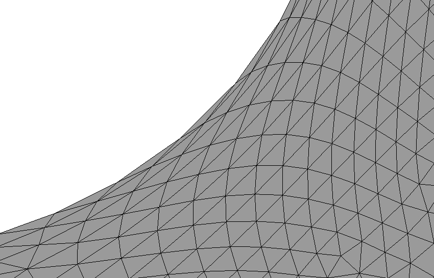
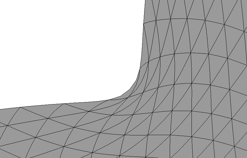
One advantage of this strategy is that a ill-shaped mesh can easily be repaired by a call of the method
mesh.ngmesh.OptimizeMesh2d() followed by
mesh.ngmesh.Update(). Figure 3 shows a ill-shaped mesh and the result of a call of mesh.ngmesh.OptimizeMesh2d().
 |
 |
6.3 Newton’s method for unconstrained problems
The particular choice and
| (63) |
for a given shape function leads to Newton’s method. We refer to a_NORO_2002a ; a_ALCAVI_2016a ; a_PAST_2019a ; a_EPHASC_2007a where shape Newton methods were used previously and to (b_HIULUL_2009a, , Chapter 2) and (b_ITKU_2008a, , Chapter 5) for Newton’s method in an optimal control setting. This bilinear form is only positive semi-definite on since for with on . Moreover, from the structure theorem for second shape derivatives proved in a_NOPI_2002a we know that at a stationary point , that is, for all , we have
| (64) |
where is a bilinear function. Hence we also have for all such that . As a result the gradient
| (65) |
according to (63) is not uniquely determined. To get around this difficulty, the shape Hessian is often regularised by an term, i.e. (63) is replaced by
| (66) |
see, e.g. a_SC_2018a , which, however, impairs the convergence speed of Newton’s method.
Alternative regularisation strategy.
Here, we propose the following strategy: We regularise the shape Hessian only on the boundary and only in tangential direction, i.e., we choose
| (67) |
with a regularisation parameter . To exclude the part of the kernel corresponding to interior deformations, we solve the (regularised) Newton equation (65) only on the boundary . This is realised by setting Dirichlet boundary conditions for all degrees of freedom except those on the boundary.
As a result, we get a shape gradient which is nonzero only on the boundary. We extend this vector field to the interior by solving an additional boundary value problem (of linearised elasticity type), where we use the deformation given by as Dirichlet boundary conditions.
The Newton algorithm reads as follows.
6.4 Newton’s method for PDE-constrained problems
We consider the PDE-constrained model problem of Section 4.1 which is subject to the Poisson equation. The unregularised Newton system reads
| (68) |
In Subsection 4.3 we discussed how the second order shape derivative can be evaluated along a fixed given direction. In this section, we want to assemble the whole shape Hessian and eventually solve a regularised version of (68). Recalling that with we see that (47) and (43) lead to
| (69) |
with
| (70) |
The component then represents the direction which we use for the shape Newton optimisation step. The matrix in (69) can be realised in NGSolve by using a combined finite element space X3 consisting of three components as follows:
The right hand side of (69) can be defined as follows:
Recall that the system (65) has a nontrivial kernel as discussed in Section 6.3. This problem can be circumvented by proceeding like in the unconstrained case. We add a regularisation only on the boundary,
and exclude the interior degrees of freedom in the first row and column of the 33 block system. This can be realised by setting Dirichlet boundary conditions for the interior degrees of freedom, i.e. by dealing with the free degrees of freedom,
and solving the regularised system using these free dofs:
The newton direction is then given as the first of the three components of the obtained solution.
7 Numerical Experiments
In this section we first verify the copmuted shape derivatives by performing a Taylor test, and then apply the automated shape differentiation and the numerical algorithms introduced in the preceding sections in numerical examples.
7.1 Code verification
We verify the expressions that we obtained in a semi-automatic or fully automatic way for the first and second order shape derivatives by looking at the Taylor expansions of the perturbed shape functionals. We illustrate our findings in two examples in . On the one hand, we consider a shape function as introduced in (6) with an additional boundary integral as in (13), henceforth denoted by ; on the other hand, we consider the PDE-constrained shape optimisation problem defined by (28), the reduced form of which will be denoted by . More precisely, we consider
| (71) | ||||
| (72) |
In the case of , we used the function
and for , we used and for the function in the PDE constraint (28b).
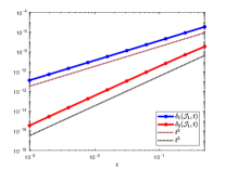
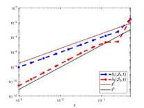
For the test of the first order shape derivatives we choose a fixed shape and a vector field and observe the quantity
| (73) |
for . Likewise, for the second order shape derivative, we consider the remainder
as . By the definition of first and second order shape derivatives, it must hold that
| (74) |
This behavior can be observed in Figure 4(a) for and in Figure 4(b) for , where we used in both cases.
 |
 |
| (a) | (b) |
The experiments for shape function was conducted on a mesh consisting of 13662 vertices, 26946 elements and with polynomial order 2 (resulting in 54269 degrees of freedom), and the experiment for with 95556 vertices and 190062 elements and polynomial degree 1 (95556 degrees of freedom). We conducted these experiments for a number of different problems with different vector fields , in particular with different PDE constraints and boundary conditions, and obtained similar results in all instances provided a sufficiently fine mesh was used.
7.2 A first shape optimisation problem
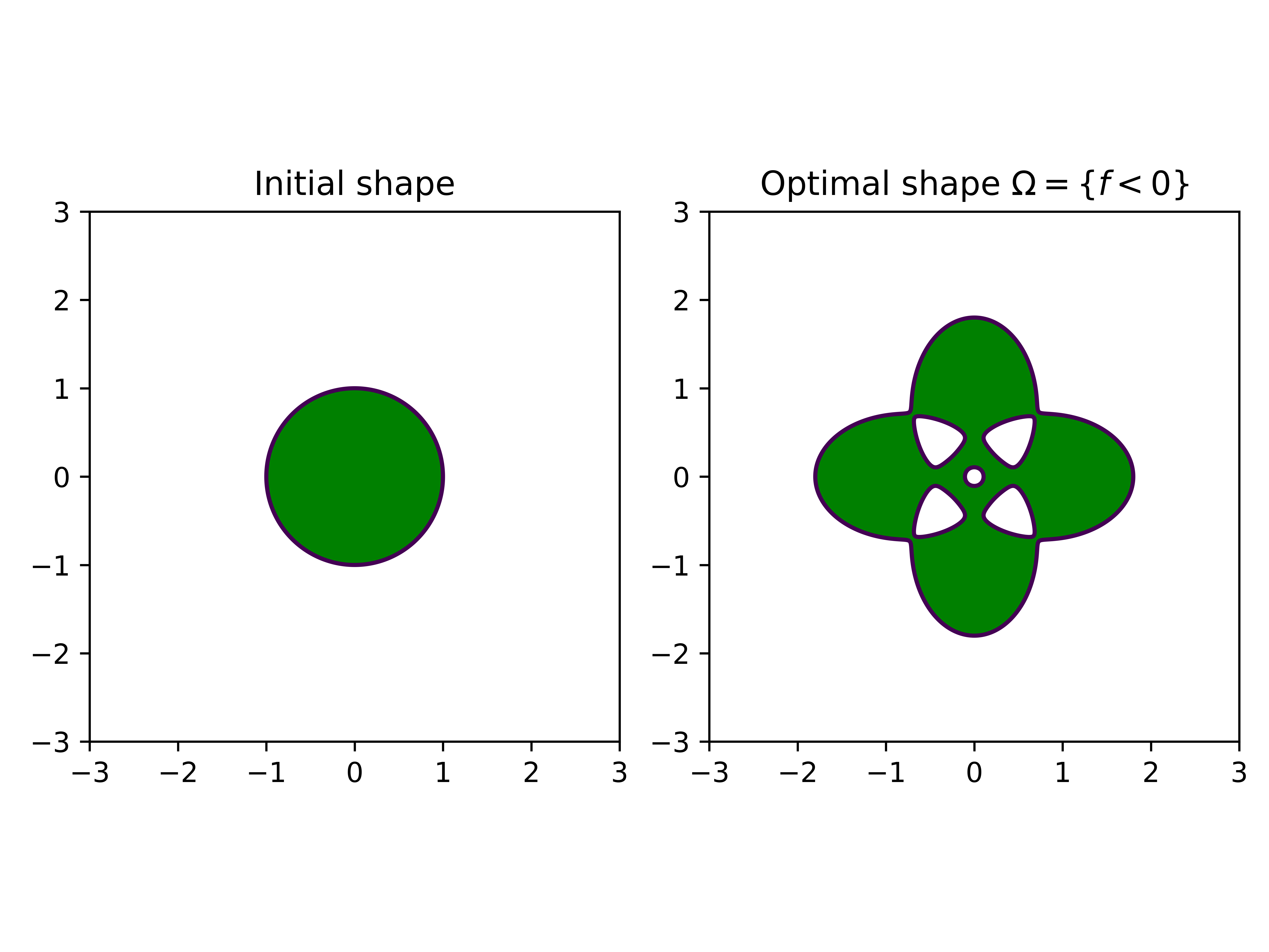
In this section, we revisit problem (6) introduced in Section 3, i.e. the problem of finding a shape such that the cost function is minimised.
7.2.1 First order methods
We illustrate our first order methods in a problem which was also considered in a_IGSTWE_2018a and reproduce the results obtained there. We choose the function
| (75) |
with , and . Recall that the optimal shape is given by which is depicted in Figure 5 (right). We start our optimisation algorithm with the unit disk, as an initial design. Note that the optimal design cannot be reached by means of shape optimisation using boundary perturbations. However, we expect the outer curve of the optimal shape to be reached very closely.
We apply Algorithm 1 with the shape gradient associated to the inner product (59), to the bilinear form of linearised elasticity (60) and including the additional Cauchy-Riemann term (61). We chose the algorithmic parameters , , a mesh consisting of 2522 vertices and 4886 elements and a globally continuous vector-valued finite element space VEC of order 3. The results can be seen in Figures 6, 7 and 8, respectively.
 |
 |


7.2.2 Second order method
Since Newton’s method converges quadratically only in a neighborhood of the optimal solution, we choose a simpler optimal design here. We choose
| (76) |
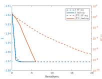
which yields an ellipse with the lengths of the two semi-axes and . We choose and and again start the optimisation with the unit disk as initial shape. Figure 9 shows the initial and optimised design after only six iterations of Algorithm 2 with chosen as in (67) with . A comparison of the convergence histories between the choice (67) with and (66) with is shown in the right picture of Figure 9. In both cases, we tested a range of different values for and compared the convergence histories for the values which yielded the fastest convergence. The experiments were conducted on a finite element mesh consisting of 2522 nodes and 4886 triangular elements with a finite element space VEC of order 3, with the algorithmic parameter .


7.3 Shape optimisation subject to the Poisson equation
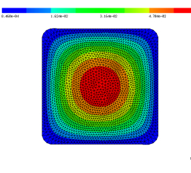
In this section, we revisit the model problem introduced in Section 4.1 with and . Note that the data is chosen in such a way that, for it holds and thus is a global minimiser of . We show results obtained by first and second order shape optimisation methods exploiting automated differentiation.
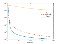
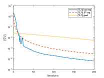
We ran the optimisation algorithm in three versions. On the one hand, we applied a first order method with constant step size . On the other hand, we applied two second order methods with the two different regularisation strategies for the shape Hessian in (65) introduced in (66) and (67). We chose the regularisation parameters empirically such that the method performs as well as possible. In the case of (66) we chose and in the case of (67) . The experiments were conducted on a finite element mesh consisting of 4886 elements with 2522 vertices and polynomial degree 1. In Figure 10, we can observe the decrease of the objective function as well as of the norm of the shape gradient over 200 iterations for these three algorithmic settings.
Figure 10 shows the initial design as well as the design after 200 iterations of the second order method with regularisation strategy (67). Note that the improved design is very close to , which is a global solution. The initial design was chosen as the disk of radius centered at the point . The objective value was reduced from to .
7.4 Nonlinear elasticity
Here, we illustrate the applicability of the automated shape differentiation and optimisation in the more realistic and more complicated setting of nonlinear elasticity in two space dimensions using a Saint Venant–Kirchhoff material with Young’s modulus and Poisson ratio . We consider a two-dimensional cantilever which is clamped on the upper and lower left parts of the boundary, and , respectively, and is subject to a surface force on . The initial geometry with 3 holes is depicted in Figure 12 (a). Let and the subspace of with vanishing trace on . The displacement under the surface force is given as the solution to the boundary value problem
| (77) |
for all . Here, denotes the Saint Venant–Kirchhoff stress tensor
| (78) |
where and is the identity matrix, see also (AllaireJouveToader2004, , Sec. 8), and and denote the Lamé constants,
| (79) |
We minimise the functional
| (80) |
with subject to (77) which amounts to maximising the structure’s stiffness while bounding the allowed amount of material used.
We remark that the well-posedness of (77) is not clear, see also the discussion in (AllaireJouveToader2004, , Sec. 8). Nevertheless, application of the automated shape differentiation and optimisation yields a significant improvement of the initial design. The highly nonlinear PDE constraint (77) is solved by Newton’s method. In order to have good starting values, a load stepping strategy is employed, i.e., the load on the right hand side is gradually increased, the PDE is solved and the solution is used as an initial guess for the next load step. This is repeated until the full load is applied. With these ingredients at hand, Algorithm 1 (i.e. code lines 106–146) can be run. We chose the algorithmic parameters alpha = 0.1 (as an initial value), alpha_incr_factor = 1 (i.e. no increase), gamma = 1e-4 and epsilon = 1e-7. Moreover, we used (59) with an additional Cauchy-Riemann term as in (61) with weight . The objective value was reduced from to (volume term from to ) in 15 iterations of Algorithm 1. The results were obtained on a mesh consisting of 10614 elements and 5540 vertices using piecewise linear, globally continuous finite elements.
| (a) | (b) | (c) |
7.5 Helmholtz equation
In this section, we consider the problem of finding the optimal shape of a scattering object. More precisely, we consider the minimisation of the functional
| (81) |
subject to the Helmholtz equation with impedance boundary conditions on the outer boundary: Find such that
| (82) |
for all . Here, denotes the complex conjugate of a complex-valued function , denotes the wave number, denotes the complex unit and the function on the right hand side is chosen as
| (83) |
see Figure 13(a). Furthermore,
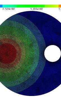
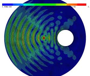
denotes the domain of interest, the outer boundary and the right half of the outer boundary. Here, only the inner boundary is subject to the shape optimisation. Thus, the aim of this model problem is to find a shape of the scattering object such that the waves are reflected away from .
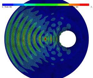
Figure 13 (b) and (c) show the initial and final shape of the scattering object, respectively. Figure 14 shows the norm of the state for the initial configuration (circular shape of scattering object) and for the optimised configuration. The objective value was reduced from to . The forward simulations were performed using piecewise linear finite elements on a triangular grid consisting of with 34803 degrees of freedom. The optimisation stopped after 12 iterations.
 |
||
| (a) | (b) | (c) |
 |
 |
| (a) | (b) |
7.6 Application to an Electric Machine
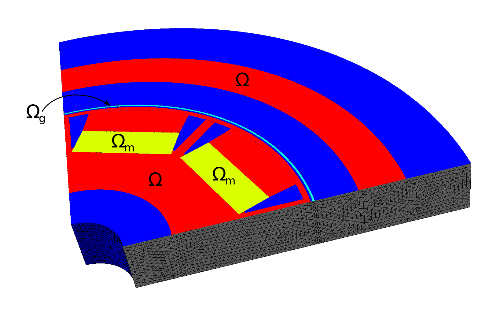
In this section, we consider the setting of three-dimensional nonlinear magnetostatics in as it appears in the simulation of electric machines. Let denote the computational domain, which consists of ferromagnetic material, air regions and permanent magnets, see Figure 15. Our aim is to minimise the functional
| (84) |
where denotes the air gap region of the machine, denotes an extension of the normal vector to the interior of , is a given smooth function and is the solution to the boundary value problem
| (85) |
for all . Here, denotes the union of the ferromagnetic parts of the electric machine, denotes the permanent magnets subdomain and
| (86) |
denotes the magnetic reluctivity, which is a nonlinear function inside the ferromagnetic regions and equal to a constant elsewhere. Further, is a small regularisation parameter and denotes the magnetisation in the permanent magnets. The nonlinear function satisfies a Lipschitz condition and a strong monotonicity condition such that problem (85) is well-posed. The goal of minimising the cost function (84) is to obtain a design which exhibits a smooth rotation pattern. Note that in this particular example we do not consider rotation of the machine, but rather a fixed rotor position, and there are no electric currents present. We refer the reader to (GanglSturm2019, , Sec. 6) for a more detailed description of the problem and to GLLMS2015 for a 2D version of the same problem.
 |
As mentioned in Section 4, the transformation used in (25) depends on the differential operator. For the curl-operator, we have
see e.g. (Monk2003, , Section 3.9). Thus, the variational equation (85) can be defined as follows.
Here, the computational domain consists of a subdomain representing the ferromagnetic part of the machine (‘‘iron’’) and a subdomain comprising the permanent magnets (‘‘magnets’’); the union of all air subdomains, including the air gap between rotating and fixed part of the machine, is given by ‘‘air|airgap’’, see Figure 15.
Moreover, nuIron denotes the nonlinear reluctivity function and magn contains the magnetisation direction of the permanent magnets. Likewise, the objective function can be defined as follows,
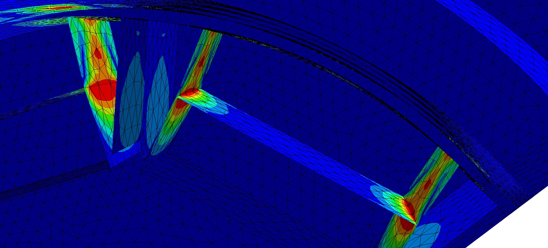
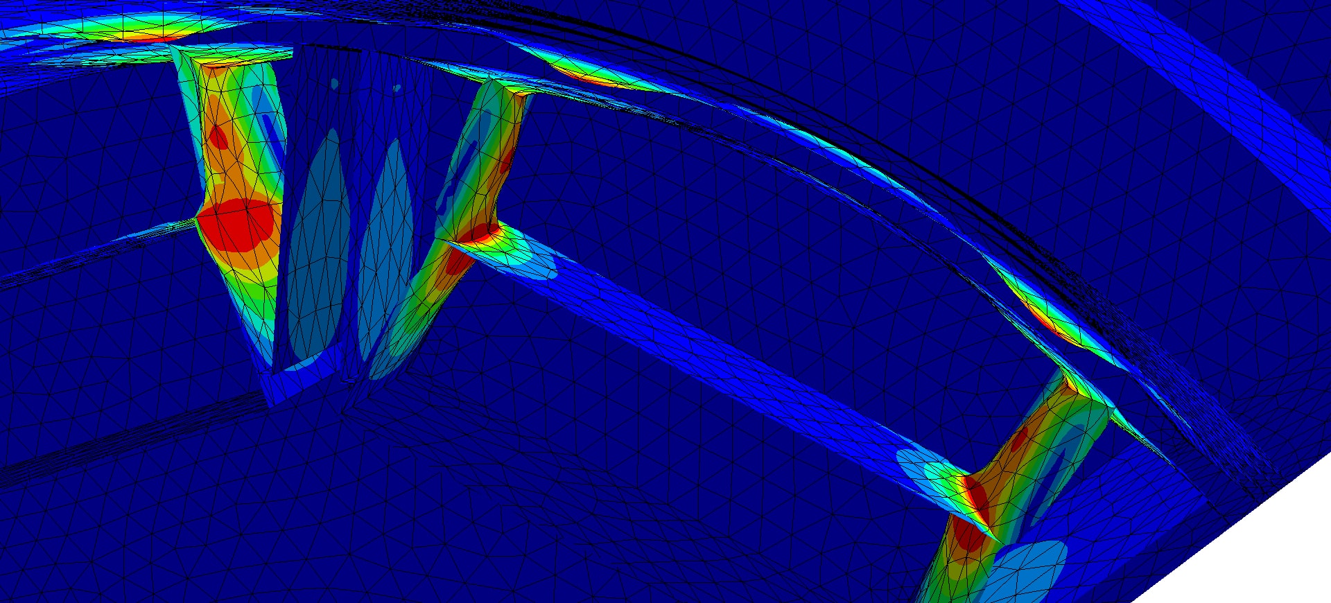
where n2D and Bd represent the extension of the normal vector to the interior of the air gap and the desired curve, respectively. For the definition of all quantities, we refer the reader to Online Resource 1. The shape differentiation as well as the optimisation loop now works in the same way as in the previous examples. Figure 16 shows the initial design of the motor as well as the optimised design obtained after 11 iterations of Algorithm 1 with . The experiment was conducted using a tetrahedral finite element mesh consisting of 13440 vertices, 57806 elements and Nédélec elements of order 2 (resulting in a total of 323808 degrees of freedom). The objective value was reduced from to in the course of the first order optimisation algorithm after 11 iterations. It can be seen from Figure 17 that the difference between the quantity and the desired curve inside the air gap decreases significantly.
 |
 |
| (a) | (b) |
| (a) | (b) | (c) |
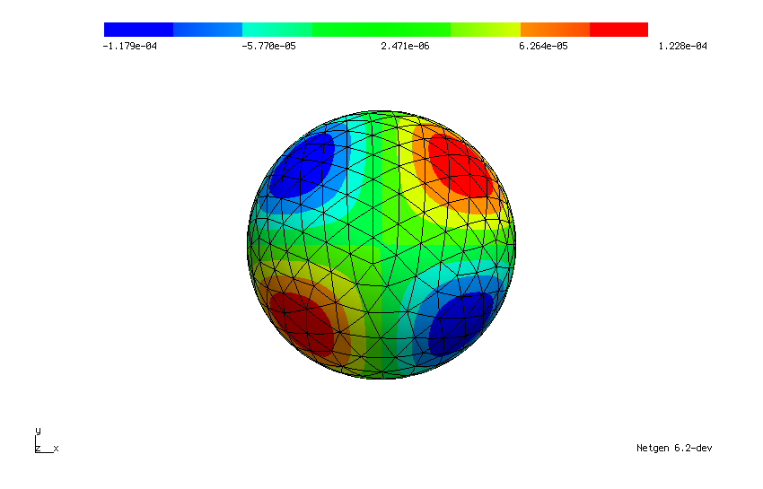
7.7 Surface PDEs
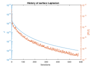
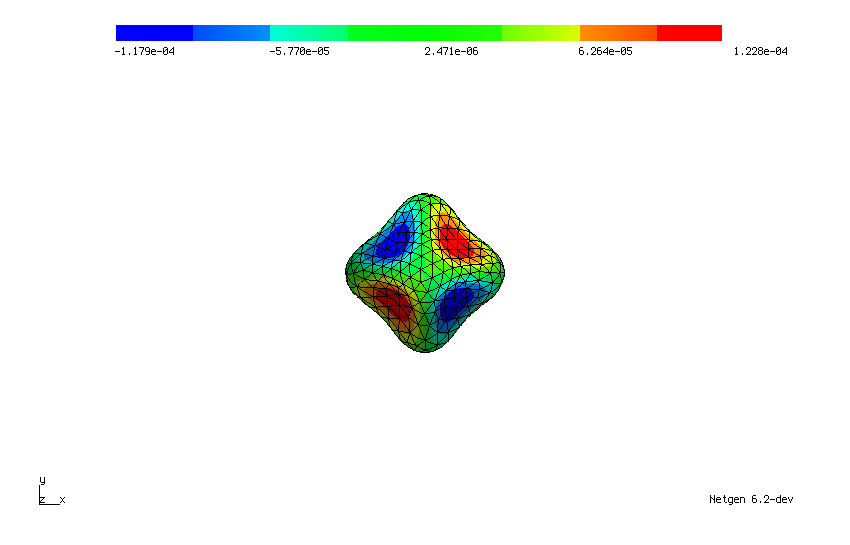
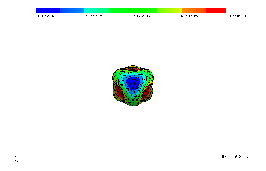
Next, we also show the application of a shape optimisation algorithm to a problem constrained by a surface PDE. We solve problem (48)–(49) with , and initial shape the unit sphere in . We applied a first order algorithm with a line search. Figure 18 shows the initial geometry as well as the decrease of the objective function and of the norm of the shape gradient. The objective value was reduced from to . Figure 19 shows the final design which was obtained after 575 iterations from two different perspectives. The experiment was conducted using a surface mesh with 332 vertices and 660 faces and polynomial degree 3 (resulting in 2972 degrees of freedom).
 |
 |
| (a) | (b) |
 |
 |
| (a) | (b) |
7.8 Time-dependent PDE using space-time method
In this section we illustrate a non-standard situation where the fully automated shape differentiation using the command .DiffShape() fails, but the semi-automated way can be used to compute the shape derivative.
The situation is that of a parabolic PDE constraint in a space-time setting where the time variable is considered as just another space variable. Let and be given and define the space-time cylinder . For given smooth functions and defined on , we consider the problem
| (87a) | ||||
| (87b) | ||||
for all in the Bochner space where the state is to be sought in the Bochner space with the initial condition . Here, denotes the spatial gradient and the time derivative. Note that we denote the time variable by in order not to interfere with the shape parameter . We refer the interested reader to Steinbach2015 for details on this space-time formulation of the PDE constraint. As it is outlined there, the PDE can be solved numerically by choosing the same ansatz and test space consisting of piecewise linear and globally continuous finite element functions on .
For simplicity, we restrict ourselves to the case where , i.e. to the case where the spatial domain is an interval. We are interested in the shape derivative of problem (87) with respect to spatial perturbations, i.e., with respect to transformations of the form
where and . We recall the notation . By this choice of transformation we exclude an unwanted deformation of the space-time cylinder into the time direction as the time horizon is assumed to be fixed.
Following the lines of the previous examples, we can define the cost function, the PDE and the Lagrangian:
Here, gfu denotes the solution to the state equation (87b) and gfp the solution to the adjoint equation, which is posed backward in time and reads in its strong form,
We can compute the shape derivative similarly to the previous examples by means of formula (10), i.e.,
| (88) |
However, it must be noted that in this special situation we have
| (93) |
The shape derivative can now be obtained as follows: Given a mesh of the space-time cylinder , we define an -valued -space to represent the vector field (here we assumed , thus we are facing a scalar-valued space). The shape derivative is a linear functional on this space and is obtained by plugging in (93) into (88):
Remark 7
The fully automated shape differentiation command .DiffShape(V) cannot be used here because the vector field has less components than the dimension of the mesh. On the other hand, if was chosen as a vector field with components, the command .DiffShape(V) would evaluate formula (88), but would assume and
and could not take into account the special situation at hand as shown in (93). This example is meant to illustrate the greater flexibility of the semi-automated compared to the fully automated shape differentiation.
Code lines 142-145 show the computation of the shape derivative in the direction of an -valued function (recall here). However, using -dependent vector fields would result in time-dependent optimal shapes, which is often not desired. Rather, one is interested in vector fields of the form which still yield a descent, i.e. . This can be achieved as follows:
-
1.
Compute a time-dependent shape gradient by solving
(94) -
2.
Set .
Note that is constant in . Then we see by plugging in in (94) that
thus is a descent direction.
We used this strategy to solve problem (87) for with the data , numerically starting out from the initial domain and the fixed time interval . Note that the data is chosen such that the domain is a global solution to problem (87).
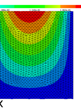
Figure 20 shows the initial design together with the solution to the state equation and the time-dependent descent vector field obtained as solution of (94). Figure 21(a) shows the averaged vector field which is independent of and yields a uniform deformation of the space-time cylinder. The final design after 293 iterations can be seen in Figure 21(b). The cost function was reduced from to .
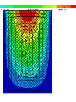 |
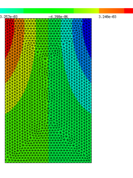 |
| (a) | (b) |
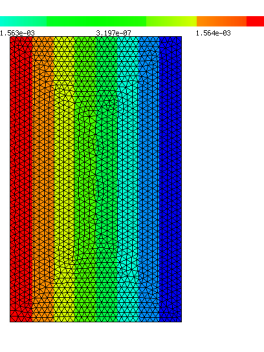 |
 |
| (a) | (b) |
For more details on the implementation of this example, we refer to Online Resource 1 and for more details on shape optimisation in a space-time setting, we refer the interested reader to master_CK .
Conclusion
We showed how to obtain first and second order shape derivatives for unconstrained and PDE-constrained shape optimisation problems in a semi-automatic and fully automatic way in the finite element software package NGSolve. We verified the proposed method numerically by Taylor tests and by showing its successful application to several shape optimisation problems. We believe that this intuitive approach can help research scientists working in the field of shape optimisation to further improve numerical methods on the one hand, and product engineers working with NGSolve to design devices in an optimal fashion on the other hand.
Acknowledgements
Michael Neunteufel has been funded by the Austrian Science Fund (FWF) project W1245. Moreover, we would like to thank Christian Köthe for his contribution to Section 7.8.
Replication of results
The python scripts which were used for the results presented in this paper are available in Online Resource 1. All computations were performed using NGSolve version V6.2.2004.
Conflicts of interest/Competing interests
On behalf of all authors, the corresponding author states that there is no conflict of interest.
References
- (1) G. Allaire. Conception optimale des structures. Springer, New York, 2007.
- (2) G. Allaire, E. Cancès, and J. L. Vié. Second-order shape derivatives along normal trajectories, governed by Hamilton-Jacobi equations. Structural and Multidisciplinary Optimization, 54(5):1245–1266, 2016.
- (3) G. Allaire, C. Dapogny, and F. Jouve. Shape and topology optimization. to appear in Handbook of Numerical Analysis, 20, 2020.
- (4) G. Allaire, F. Jouve, J., and A.-M. Toader. Structural optimization using sensitivity analysis and a level-set method. Journal of Computational Physics, 194(1):363 – 393, 2004.
- (5) M. S. Alnæs, A. Logg, K. B. Ølgaard, M. E. Rognes, and G. N. Wells. Unified form language. ACM Transactions on Mathematical Software, 40(2):1–37, 2014.
- (6) M. Berggren. A unified discrete-continuous sensitivity analysis method for shape optimization. In Applied and numerical partial differential equations, volume 15 of Comput. Methods Appl. Sci., pages 25–39. Springer, New York, 2010.
- (7) M. Burger. A framework for the construction of level set methods for shape optimization and reconstruction. Interfaces and Free Boundaries, 5:301–329, 2002.
- (8) F. de Gournay. Velocity extension for the level-set method and multiple eigenvalues in shape optimization. SIAM Journal on Control and Optimization, 45(1):343–367, jan 2006.
- (9) M. C. Delfour and J.-P. Zolésio. Shapes and geometries, volume 22 of Advances in Design and Control. Society for Industrial and Applied Mathematics (SIAM), Philadelphia, PA, second edition, 2011. Metrics, analysis, differential calculus, and optimization.
- (10) M. C. Delfour and J. P. Zolésio. Shapes and geometries. Society for Industrial and Applied Mathematics, 2011.
- (11) L Demkowicz. Projection-based interpolation. ICES Report, 4(3):1–22, 2004.
- (12) J. S. Dokken, S. K. Mitusch, and S. W. Funke. Automatic shape derivatives for transient PDEs in FEniCS and Firedrake. arXiv e-prints, page arXiv:2001.10058, 2020.
- (13) K. Eppler, H. Harbrecht, and R. Schneider. On convergence in elliptic shape optimization. SIAM Journal on Control and Optimization, 46(1):61–83, 2007.
- (14) L. Evans. Partial differential equations. American Mathematical Society, Providence, R.I, 2010. With the collaboration of Marc Schoenauer (INRIA) in the writing of Chapter 8.
- (15) F. Feppon, G. Allaire, F. Bordeu, J. Cortial, and C. Dapogny. Shape optimization of a coupled thermal fluid-structure problem in a level set mesh evolution framework. SeMA, 76(3):413–458, 2019.
- (16) P. Gangl, U. Langer, A. Laurain, H. Meftahi, and K. Sturm. Shape optimization of an electric motor subject to nonlinear magnetostatics. SIAM Journal on Scientific Computing, 37(6):B1002–B1025, 2015.
- (17) P. Gangl and K. Sturm. Asymptotic analysis and topological derivative for 3D quasi-linear magnetostatics, 2019. arXiv:1908.10775.
- (18) D. A. Ham, L. Mitchell, A. Paganini, and F. Wechsung. Automated shape differentiation in the unified form language. Structural and Multidisciplinary Optimization, 60(5):1813–1820, 2019.
- (19) A. Henrot and M. Pierre. Variation et optimisation de formes : une analyse géométrique. Springer, Berlin New York, 2005.
- (20) M. Hintermüller and A. Laurain. Electrical impedance tomography: from topology to shape. Control and Cybernetics, 37(4):913–933, 2008.
- (21) M. Hinze, R. Pinnau, M. Ulbrich, and S. Ulbrich. Optimization with PDE constraints. Springer, New York, 2009.
- (22) R. Hiptmair, A. Paganini, and S. Sargheini. Comparison of approximate shape gradients. BIT, 55(2):459–485, 2015.
- (23) D. Hömberg and J. Sokolowski. Optimal shape design of inductor coils for surface hardening. SIAM Journal on Control and Optimization, 42(3):1087–1117, 2003.
- (24) J. A. Iglesias, K. Sturm, and F. Wechsung. Two-dimensional shape optimization with nearly conformal transformations. SIAM Journal on Scientific Computing, 40(6):A3807–A3830, 2018.
- (25) K. Ito and K. Kunisch. Lagrange multiplier approach to variational problems and applications. Society for Industrial and Applied Mathematics, Philadelphia, PA, 2008.
- (26) C. Köthe. PDE-constrained shape optimization for coupled problems using space-time finite elements. Master’s thesis, Graz University of Technology, 2020.
- (27) A. Laurain. A level set-based structural optimization code using FEniCS. Structural and Multidisciplinary Optimization, 58(3):1311–1334, 2018.
- (28) P. Monk. Finite element methods for Maxwell’s equations. Numerical Mathematics and Scientific Computation. Clarendon Press, 2003.
- (29) F. Murat and J. Simon. Sur le contrôle par un domaine géométrique. Rapport 76015, Université Pierre et Marie Curie, Paris, 1976.
- (30) A. Novruzi and M. Pierre. Structure of shape derivatives. Journal of Evolution Equations, 2(3):365–382, 2002.
- (31) A. Novruzi and J. R. Roche. Newton’s method in shape optimisation: A three-dimensional case. Bit Numerical Mathematics, 40(1):102–120, 2000.
- (32) A. Paganini, S. Sargheini, R. Hiptmair, and Ch. Hafner. Shape optimization of microlenses. Optics Express, 23(10):13099, 2015.
- (33) A. Paganini and K. Sturm. Weakly normal basis vector fields in RKHS with an application to shape Newton methods. SIAM Journal on Numerical Analysis, 57(1):1–26, 2019.
- (34) A. Schiela and J. Ortiz. Second order directional shape derivatives, March 2017.
- (35) S. Schmidt. A two stage CVT / eikonal convection mesh deformation approach for large nodal deformations. arXiv e-prints, page arXiv:1411.7663, 2014.
- (36) S. Schmidt. Weak and strong form shape Hessians and their automatic generation. SIAM Journal on Scientific Computing, 40(2):C210–C233, 2018.
- (37) S. Schmidt, C. Ilic, V. Schulz, and N. Gauger. Three-dimensional large-scale aerodynamic shape optimization based on shape calculus. AIAA Journal, 51(11):2615–2627, 2013.
- (38) S. Schmidt, C. Ilic, V. Schulz, and N. R. Gauger. Airfoil design for compressible inviscid flow based on shape calculus. Optimization and Engineering, 12(3):349–369, 2011.
- (39) J. Schöberl. C++11 implementation of finite elements in NGSolve. Technical Report 30, Institute for Analysis and Scientific Computing, Vienna University of Technology, 2014.
- (40) V. H. Schulz. A riemannian view on shape optimization. Foundations of Computational Mathematics, 14(3):483–501, 2014.
- (41) J. Simon. Second variations for domain optimization problems. Control theory of distributed parameter systems and applications, 91:361–378, 1989.
- (42) J. Sokołowski and J.-P. Zolésio. Introduction to shape optimization, volume 16 of Springer Series in Computational Mathematics. Springer-Verlag, Berlin, 1992. Shape sensitivity analysis.
- (43) O. Steinbach. Space-Time Finite Element Methods for Parabolic Problems. Computational Methods in Applied Mathematics, 15(4):551–566, 2015.
- (44) K. Sturm. Minimax Lagrangian approach to the differentiability of nonlinear PDE constrained shape functions without saddle point assumption. SIAM Journal on Control and Optimization, 53(4):2017–2039, 2015.
- (45) K. Sturm. Shape differentiability under non-linear PDE constraints. In New trends in shape optimization, volume 166 of Internat. Ser. Numer. Math., pages 271–300. Birkhäuser/Springer, Cham, 2015.