Superparticle Method for Simulating Collisions

Abstract

For problems in astrophysics, planetary science and beyond, numerical simulations are often limited to simulating fewer particles than in the real system. To model collisions, the simulated particles (aka superparticles) need to be inflated to represent a collectively large collisional cross section of real particles. Here we develop a superparticle-based method that replicates the kinetic energy loss during real-world collisions, implement it in an $N$-body code and test it. The tests provide interesting insights into dynamics of self-gravitating collisional systems. They show how particle systems evolve over several free fall timescales to form central concentrations and equilibrated outer shells. The superparticle method can be extended to account for the accretional growth of objects during inelastic mergers.

1 Introduction

Numerical simulations are often limited in their ability to simulate statistically large particle systems. For example, a protoplanetary disk simulation can account for $\sim 10^{8}$-10⁹ particles (and grid cells; e.g., Li et al. 2019), but the actual number of real-world elements (dust grains, boulders, etc.) is vastly larger. The simulated particles have more mass and represent a large number of real particles. We call this the superparticle method. The superparticle method has general applicability in many areas of science. Here we discuss it in the context of planet formation (see Youdin & Kenyon (2013) for a review) mainly because our previous studies of the initial stages of planet formation directly motivated this work.

During the earliest stages of planet formation, small grains condense in a protoplanetary nebula and grow to larger ice/dust aggregates by sticking to each other. The growth stalls near cm sizes because the electrostatic forces are not strong enough to hold large particles together. Also, large grains feel strong aerodynamic drag from the surrounding gas and drift toward the central star on timescales too short for significant growth to happen (e.g., Birnstiel et al. 2016, but see Michikoshi & Kokubo 2016). It is therefore quite mysterious how planet formation bridges the gap between cm-size particle aggregates (hereafter pebbles) and 1–1000 km bodies (planetesimals; Chiang & Youdin 2010, Johansen et al. 2014). A growing body of evidence now suggests that an aerodynamic interaction between pebbles and nebular gas (e.g., the streaming instability, Youdin & Goodman 2005) can collect particles in large self-gravitating clouds that then directly collapse into planetesimals.

The initial stages of particle concentrations in a gas nebula can be studied with specialized hydrocodes (e.g., ATHENA with the particle module of Bai & Stone 2010). Simulations show that the streaming instability (hereafter SI) should be particularly important (Youdin & Johansen, 2007; Johansen & Youdin, 2007; Johansen et al., 2009; Nesvorný et al., 2019; Li et al., 2019). The instability occurs because an initially small over-density of pebbles accelerates the gas. This perturbation launches a wave that amplifies pebble density as it oscillates. Strong pebble clumping eventually triggers gravitational collapse into planetesimals. Modern hydrocode simulations of the SI, however, do not have adequate spatial resolution to follow the gravitational collapse to completion. Moreover, once the pebble density within a collapsing cloud exceeds the gas density, aerodynamic effects of gas cease to be important, and detailed hydrodynamic calculations are no longer required (Nesvorný, Youdin & Richardson 2010; hereafter NYR10). Instead, one has to realistically model pebble collisions that damp random speeds and stimulate growth (Wahlberg Jansson & Johansen 2014).

In our previous work (NYR10), we studied gravitational collapse with a cosmological $N$-body code known as PKDGRAV (Stadel 2001). PKDGRAV is a scalable, parallel tree code that is the fastest code available to us for these type of calculations. A unique feature of PKDGRAV is the ability to rapidly detect and realistically treat collisions between particles (Richardson et al. 2000). In NYR10, individual PKDGRAV particles were artificially inflated to mimic a very large collisional cross section of pebbles. We simply scaled up the radius of PKDGRAV particles by a multiplication factor that was the same for all particles and unchanging with time. This is not ideal for several different reasons. Crucially, the method with fixed inflation factor does not correctly account for the kinetic energy loss during inelastic collisions.

Here we extend the superparticle method to be able to more realistically model planetesimal formation (Section 3). The new method is designed to reproduce the kinetic energy loss. It will be useful in many areas of science where particle collisions and energy dissipation are important. The method is tested for self-gravitating collisional systems in Section 4. To provide some background for these tests, we discuss several relevant timescales in Section 2. Section 5 summarizes our findings.

2 Collision and collapse timescales

2.1 Collisions

Here we define the collisional timescale, $t_{\rm coll}$, as the timescale on which any particle in a cloud would, on average, have one collision with another particle. The collisional timescale is then $t_{\rm coll}=1/\eta\sigma v$, where $\eta$ is the number density of particles, $\sigma=\pi r^{2}$ is the particle cross-section, $r$ is the particle radius, and $v$ is the relative speed. Adopting the virial speed $v=(GM/R)^{1/2}$, where $G$ is the gravitational constant and $M$ and $R$ are the mass and radius of the cloud, we obtain

$$t_{\rm coll}={4\over 3nr^{2}\sqrt{GM}}R^{7/2}\ ,$$ (1)

where $n$ is the total number of cloud particles. The collisional timescale is therefore a steep function of cloud’s size. We assume that the cloud radius is some fraction of the Hill radius, $R=f_{\rm H}R_{\rm H}$, where

$$R_{\rm H}=a\left({M\over 3M_{\odot}}\right)^{1/3}\ ,$$ (2)

$a$ is the orbital radius, and $M_{\odot}\simeq 2\times 10^{33}$ g is the solar mass. After substituting for $R_{\rm H}$ and $n=(R_{\rm eq}/r)^{3}$, where $R_{\rm eq}$ is the equivalent radius of a sphere with mass $M$ and density 1 g cm^-3, we obtain

$$t_{\rm coll}\simeq 23\,{\rm yr}\ \left({r\over 1\,{\rm cm}}\right)\left({50\ {\rm km}\over R_{\rm eq}}\right)\left({f_{\rm H}\over 0.5}\,{a\over 45\,{\rm au}}\right)^{7/2}\ .$$ (3)

For comparison, the orbital period at 45 au is $P\simeq 300$ yr. This illustrates the importance of particle collisions. Collisions will act to damp particle speeds and stimulate growth.

2.2 Virial collapse

In virial equilibrium, $T=-U/2$, where $T=\sum_{i}m_{i}v_{i}^{2}/2$ and $U=-\sum_{i,j}Gm_{i}m_{j}/r_{ij}$, with $r_{ij}=|\mathbf{r}_{i}-\mathbf{r}_{j}|$, are the total kinetic and potential energies of particles with masses $m_{i}$, positions $\mathbf{r}_{i}$ and speeds $v_{i}$. If a cloud is in virial equilibrium, it cannot collapse unless some dissipative process, such as inelastic collisions between particles, reduces the kinetic energy. In a single collision of two pebbles with masses $m_{i}^{\prime}$ and $m_{j}^{\prime}$, the change in energy is

$$\delta E=-{1\over 4}\mu\Delta v^{2}(1-C^{2}_{\rm R})\ ,$$ (4)

where $\mu=m_{i}^{\prime}m_{j}^{\prime}/(m_{i}^{\prime}+m_{j}^{\prime})$, $\Delta v$ is the collision speed and $C_{\rm R}$ is the coefficient of restitution. The above equation takes into account that collisions are not necessarily head-on, which reduces the average dissipated energy by a factor of 1/2.

Assuming that all particles have the same mass and $\Delta v=\sqrt{2}\,v$, where $v=(GM/R)^{1/2}$ is the virial speed, the total energy lost in the time interval $\Delta t$ is

$$\Delta E=\delta E\times n{\Delta t\over t_{\rm coll}}\ ,$$ (5)

where $n$ is the number of particles and $t_{\rm coll}$ is given in Eq. (1). This leads to a differential equation for the total energy of the cloud, $E$, or equivalently, for the cloud radius. Wahlberg Jansson & Johansen (2014) showed that

$$E=E_{0}\left(1-{t\over t_{\rm vir}}\right)^{-2/7}\ ,$$ (6)

where $t$ is time and $E_{0}$ is the initial energy. This assumes that frequent collisions instantaneously virialize the cloud. The virial collapse timescale $t_{\rm vir}$ is given by

$$t_{\rm vir}=0.26\,t_{\rm coll}(1-C^{2}_{\rm R})^{-1}$$ (7)

with $t_{\rm coll}$ in Eq. (1). The virial collapse timescale is thus roughly four times shorter for $C_{\rm R}=0$ than the collisional timescale for $t=0$. This is a consequence of the steep dependence of $t_{\rm coll}$ on $R$. In the virial collapse, the cloud radius $R$ is related to Eq. (6) via

$$R={3GM^{2}\over 10E}\ .$$ (8)

2.3 Free fall collapse

The above analysis is valid when the collapse is “hot”, i.e., when particle speeds are virial and remain virial during the whole collapse. An alternative to this is the “cold” collapse with sub-virial particle speeds. In this case, the collapse timescale is related to the free fall timescale

$$t_{\rm free}=\left({3\pi\over 32G\rho_{\rm cloud}}\right)^{1/2}\ ,$$ (9)

where $\rho_{\rm cloud}=3M/4\pi R^{3}$ is the cloud’s mass density. This assumes that particles have negligible initial velocities and collisions are ignored. If the mass is uniformly distributed within a spherical volume of radius $R$, the collapse is self-similar and all radial shells shrink on the timescale given by Eq. (9). If the mass is initially concentrated toward the cloud’s center, the inner shells will infall faster than the outer shells.

Substituting $\rho_{\rm cloud}$ and $R=f_{\rm H}R_{\rm H}$ into Eq. (9), we obtain

$$t_{\rm free}=11\,{\rm yr}\ \left({f_{\rm H}\over 0.5}\,{a\over 45\,{\rm au}}\right)^{3/2}\ ,$$ (10)

which is independent of $M$ (or $R_{\rm eq}$), because more massive clouds have larger Hill radii and these dependencies cancel out in $\rho_{\rm cloud}$. Thus, in our fiducial case with $f_{\rm H}=0.5$, $a=45$ au, $r=1$ cm, $R_{\rm eq}=50$ km and $C_{\rm R}=0$, we obtain $t_{\rm vir}<t_{\rm free}$, which shows that collisions damp the random velocities faster than the cloud can collapse. The collapse will thus happen on the free fall timescale. Given the different scaling of Eqs. (3) and (10) with $R_{\rm eq}$, only small clouds with $R_{\rm eq}<25$ km can, at least initially, contract on the $t_{\rm vir}$ timescale. As $t_{\rm coll}$ drops faster during the collapse than $t_{\rm free}$, however, all clouds will eventually free fall.

3 Superparticle method

Two particle systems are considered here: one that consists of real particles (RPs) and another one that consists of simulated superparticles (SPs). Inelastic collisions between particles happen in both systems. They can result in inelastic bounces or mergers of particles, and the loss of kinetic energy. We assume that the number of SPs is much smaller than the number of RPs, and ask how to best deal with collisions in the SP system such as it statistically reproduces the behavior (i.e., energy loss, particle growth) of the RP system.

3.1 Size distributions

We denote the number distributions of SPs as $dN$ and RPs as $dN^{\prime}$. In terms of the RP radius $r$ (no prime here) we may have a size distribution $dN^{\prime}/dr\propto r^{-q}$. The number distribution of SPs can (i.e., might need to) be different, e.g. $dN/dr\propto r^{-Q}$. For instance, $Q=1$ would be a log-uniform distribution that might be a good choice to numerically sample.

We define $n(r)$ as the number of RPs replaced by a single SP, or (equivalently) the mass ratio of a SP and its RP. The mass in each bin is the same in both systems, $dM=m(r)dN=m^{\prime}(r)dN^{\prime}=n(r)m^{\prime}(r)dN$, where $m^{\prime}(r)$ is the mass of a RP. Thus

$$n(r) =dN^{\prime}/dN=m/m^{\prime}$$ (11)

and for the example of power-law distributions $n(r)\propto r^{Q-q}$ and $n(r)\propto r^{1-q}$ for log-uniform SPs. With typical $q\approx 3$–$4$, we see that the sampling rate $n(r)$ should be much larger for smaller RPs. Indeed for constant density RPs with $m^{\prime}\propto r^{3}$, our log-uniform example means that SPs for smaller $r$ will be more massive for $q>4$ (or $q>3+Q$ for other SP power-laws). We will refer to this pathological case as SP mass inversion.

More generally, for non-constant $n(r)$, the mass ratios of SPs will not be the same as the RPs they model. This may have some undesirable properties for gravitational and collisional dynamics. In particular, both gravitational scattering and (inelastic) collisions tend towards equipartition, i.e., equal kinetic energies for all species. If SPs do not have the same $n$, then we risk forcing equipartition of the artificial SP masses. Since varying $n(r)$ may be difficult to avoid, the question is whether this tendency to equipartition is significant, or whether it is over-ridden by other physics (e.g., the fact that collisions are inelastic). Moreover the timescale for equipartition could be long compared to timescales of interest (e.g., for gravitational collapse).

3.2 Inelastic collisions

Intuitively the system of SPs must have larger collisional radii than RPs to account for the reduced number. Specifically, we want the energy loss rate from collisions per unit volume, $\dot{E}$, to be the same in the RP and SP systems. For collisions between species $i$ and $j$ the differential loss rate is

$$d\dot{E}_{ij}=\frac{1}{4}dN(r_{i})dN(r_{j})\sigma_{ij}v_{ij}^{3}\mu_{ij}f(C_{\rm R})$$ (12)

for cross section $\sigma_{ij}$, relative speed $v_{ij}$, reduced mass $\mu_{ij}=m_{i}m_{j}/(m_{i}+m_{j})$ and coefficient of restitution $C_{\rm R}$. Averaged over impact angles, $f(C_{\rm R})=(1-C_{\rm R}^{2})/2$ (Section 2.2). The total $\dot{E}$ is obtained by a double integral over the size distributions for species $i$ and $j$. In more detail, the above equation is already averaged over a velocity distribution and impact angles, and the $dN$’s are now per unit volume. The 1/4 in Eq. (12) represents 1/2 from kinetic energy and 1/2 to avoid double counting of species pairs.

We now equate our (unprimed) SP system with the (primed) RP system, $d\dot{E}_{i,j}=d\dot{E}_{i,j}^{\prime}$. We assume $v_{ij}=v_{ij}^{\prime}$ and $f(C_{\rm R})=f^{\prime}(C_{\rm R})$, i.e., that the SPs have a similar velocity distribution to the RPs and there is a similar distribution of impact angles. From Equations (11) and (12) we get the desired result:

$$\sigma_{ij} =\sigma^{\prime}_{ij}\frac{m_{i}+m_{j}}{m_{i}^{\prime}+m_{j}^{\prime}}=\sigma^{\prime}_{ij}\frac{n_{i}m_{i}^{\prime}+n_{j}m_{j}^{\prime}}{m_{i}^{\prime}+m_{j}^{\prime}}\ ,$$ (13)

i.e., the cross section to mass ratio is the same for SP and RP collisions.

If SPs $i$ and $j$ represent the same number of RPs, $n_{i}=n_{j}$, then $\sigma=\sigma^{\prime}n$, i.e., the effective SP radii are $R_{i}=\sqrt{n}r_{i}$ and $R_{j}=\sqrt{n}r_{j}$. For strongly unequal true masses $m_{i}^{\prime}\gg m_{j}^{\prime}$,

$$\sigma_{ij} \xrightarrow{m_{i}^{\prime}\gg m_{j}^{\prime}}\frac{\pi r_{i}^{2}}{m_{i}^{\prime}}(m_{i}+m_{j})\ .$$ (14)

If the SP masses are not inverted, such that $m_{i}>m_{j}$, we again get $R_{i}\approx\sqrt{m_{i}/m^{\prime}_{i}}r_{i}=\sqrt{n_{i}}r_{i}$. Moreover, if we define (now relaxing the assumption of strongly unequal masses)

$$\sigma_{ij} \equiv\pi(R_{i}+R_{j})^{2}\equiv\pi(\sqrt{n_{i}}r_{i}+R_{j})^{2}\ ,$$ (15)

then $R_{j}>0$ by application of Equation (13). This result shows that even the naive estimate of $R_{i}\approx\sqrt{n_{i}}r_{i}$ is “safe” in that it won’t require negative radii for the collisional partner, i.e. the other SP.

3.3 Mergers

If SPs merge, this represents a merger of some large number of RPs. If SPs $i$ and $j$ merge to a new SP $k$, the masses simply add $m_{k}=m_{i}+m_{j}$. However there is some choice as to how the underlying true particle masses combine. We would like to exploit this choice so that SPs gradually approach RPs as coagulation proceeds. The final collapse outcome will then have more realistic densities and a more meaningful final multiplicity (single, multiple, etc.). The obvious choice of simply merging the true masses, as $m_{k}^{\prime}=m_{i}^{\prime}+m_{j}^{\prime}$, doesn’t allow this transition, as we now explain in more detail.

Our desired transition requires a gradual decrease in the sampling rates $n_{k}$. The obvious merging strategy clearly doesn’t have this property. If all SPs merge they have a total mass $m_{\rm tot}=\sum_{i}m_{i}=\sum_{i}n_{i}m_{i}^{\prime}$, while the simple sum of RP masses is $m^{\prime}_{\rm tot}=\sum_{i}m_{i}^{\prime}$ (where $i$ is now a sum over each SP and not each size bin). Clearly, the sampling rate of this final object $n_{\rm tot}=\sum_{i}n_{i}m^{\prime}_{i}/\sum_{i}m^{\prime}_{i}$ will be large if the initial $n_{i}$ are large, as this final $n_{\rm tot}$ is just a mass-weighted average of the initial $n_{i}$. Again, a decrease of the sampling rate is needed to approach a true system.

During a merger event, we thus choose to reduce the merged sampling rate $n_{k,\text{merged}}$ and thus increase the RP masses (since the SP masses must be conserved). From the merger of $m_{k}=m_{i}+m_{j}$, the post-merger sampling rate must obey

$$n_{k,\text{merged}} <\frac{m_{k}}{m^{\prime}_{i}+m^{\prime}_{j}}\equiv n_{k,0}\,,$$ (16)

where $n_{k,0}$ would arise from the obvious summation of RP masses. For instance, in Section 4.3, we consider $n_{k,\text{merged}}=\max(n_{k,0}(1-m_{j}/m_{k}),1)$ for $m_{i}>m_{j}$. (Note that this correction uses the SP masses, but we also have $m^{\prime}_{i}>m^{\prime}_{j}$ for the RP masses, provided we stick to the non-inverted samplings.)

With different merger prescriptions, we should consider how the mass growth timescales of SP and RP systems are related in theory. Recall that we are considering an SP cross section that correctly models energy dissipation but not necessarily the mass growth. To explore this issue, we consider the mass growth rate of a given SP in bin $i$ due to the SPs in bin $j$ :

$$\frac{\dot{m}_{i,j}}{m_{i}} =\frac{m_{j}}{m_{i}}dN_{j}\sigma_{ij}v_{ij}$$ (17)

and the corresponding RP growth rate (for simple addition of RP masses, i.e. before any rescaling) :

$$\frac{\dot{m}^{\prime}_{i,j}}{m^{\prime}_{i}} =\frac{m^{\prime}_{j}}{m^{\prime}_{i}}dN^{\prime}_{j}\sigma^{\prime}_{ij}v^{\prime}_{ij}=\frac{m_{j}}{m^{\prime}_{i}}dN_{j}\sigma_{ij}v_{ij}\frac{m^{\prime}_{i}+m^{\prime}_{j}}{m_{i}+m_{j}}=\frac{\dot{m}_{i,j}}{m_{i}}\left[\frac{1+m^{\prime}_{j}/m^{\prime}_{i}}{1+m_{j}/m_{i}}\right]\,.$$ (18)

Above we use our previous result for conservation of mass per bin ($m_{j}dN_{j}=m^{\prime}_{j}dN^{\prime}_{j}$), and again use the cross section relation of Equation (13) assuming accurate modeling of velocities $v_{ij}=v^{\prime}_{ij}$. Equation (18) shows that the mass growth timescales for the RP and SP systems will agree in the special case where the term in square brackets is unity. This special condition occurs (1) for uniform sampling, i.e. $n_{i}=n_{j}$, which again is often overly restrictive and (2) in the limit of very small accreted masses $j$, both for the SP and RP masses. Aside from these special conditions, mass growth rates will not agree exactly. We thus confirm that a cost of non-uniform SP sampling is that energy dissipation and mass growth can’t both be reproduced exactly.

In what direction should the inexact growth rates go? Consider $m_{i}^{\prime}>m_{j}^{\prime}$ and the standard case $n_{j}>n_{i}$ for more efficient sampling. Then Equation (18) gives $\dot{m}_{i,j}/m_{i}>\dot{m^{\prime}}_{i,j}/m^{\prime}_{i}$. In words, the large SPs will grow at a statistically larger rate than they “should” if they were accurately modeling the RP system. In practice, differences in the SP vs. RP relative velocities will also affect growth rates. Thus we must compare RP and SP growth rates numerically to asses these issues quantitatively.

3.4 PKDGRAV implementation

The method described above was implemented in the hard-sphere flavor of PKDGRAV (Richardson et al. 2000). To detect collisions, PKDGRAV sorts neighbors of each particle by distance. The particle and each neighbor are then tested for a collision during the next timestep ${\rm d}T$. The condition is simply $d_{ij}(t)\leq R_{i}+R_{j}$, where $d_{ij}(t)$ is the distance of $i$ and $j$ particles at time $0<t<dT$, and $R_{i}+R_{j}$ is the sum of particle radii. We changed the collision condition in PKDGRAV such that $R_{i}+R_{j}=\sqrt{\sigma_{ij}/\pi}$, where $\sigma_{ij}$ is given by Eq. (13). When a collision is detected, PKDGRAV decides, based on user-defined parameters, collision speed, etc., whether it results in a merger or bounce.

If a merger is applied, we use the method described in Section 3.3 to generate a new SP. PKDGRAV then computes the velocity of the new SP from the linear momentum conservation. Particle bounces in PKDGRAV are controlled by the normal coefficient of restitution, $0\leq C_{\rm R}\leq 1$, where $C_{\rm R}=0$ corresponds to a fully inelastic collision and $C_{\rm R}=1$ to an ideally elastic bounce (i.e., no energy dissipation). The code computes post-collision velocities of SP $i$ and $j$ and moves to considering a new SP pair. PKDGRAV is also capable of producing particle aggregates, where interacting particles become rigidly locked as a group, but we do not use this option here.

Specifically, we implemented the following changes in PKDGRAV:

1. We modified the structure of the input/output files such that $n_{i}$ and $r_{i}$ of each SP is given in the last two columns. New variables, fNpebble and fRpebble were included in the PKD (particle data) and COLLIDER (collision data) structures. The new variables are passed between these structures in pkdGetColliderInfo and pkdPutColliderInfo (functions to retrieve and store collision data). SSDATA_SIZE (solar system data size) in ssio.h was increased to make space for new variables. The function pkdReadSS now reads these variables from input and passes it to the PKD structure.

2. We changed the function CheckForCollision (function that tests particle’s neighbors for collision in the current timestep) in smoothfcn.c such that the sum of particle radii is ${\tt sr}=\sqrt{\sigma_{ij}/\pi}$, where $\sigma_{ij}$ is given in Eq. (13). We also modified option OverlapAdjPos (a method to deal with overlapping particles by separating them along their line of centers) in pkdDoCollision, included in collisions.c, such that the displacement is aligned with the definition of sr in CheckForCollision.

3. We implemented the merger algorithm from Sect. 3.3 in function pkdMerge, included in collisions.c. This was done in two steps to account for the merger of $i$ and $j$ SPs, and to reduce the number of RPs. In pkdBounce, the individual particle radii were replaced by $R_{i}=r_{i}\sqrt{(n_{i}m_{i}^{\prime}+n_{j}m_{j}^{\prime})/(m_{i}^{\prime}+m_{j}^{\prime})}$ and $R_{j}=r_{j}\sqrt{(n_{i}m_{i}^{\prime}+n_{j}m_{j}^{\prime})/(m_{i}^{\prime}+m_{j}^{\prime})}$. This assures that the linear momentum conservation part in pkdBounce operates with the right quantities. The SP bounces in PKDGRAV are treated as bounces of particles with inflated radii.

4. The expression for the escape velocity of colliding SPs in pkdDoCollision (function that executes collisions) was changed such that $v_{\rm esc}^{2}=2(m_{i}+m_{j})/\sqrt{\sigma_{ij}/\pi}$ with $\sigma_{ij}$ from Eq. (13). PKDGRAV uses the escape velocity and the parameter dMergeLimit to decide whether the SPs should be merged.

The modified PKDGRAV code works with the pthread parallelization and we typically used 5, 10 or 28 Broadwell cores in the tests described in Sect. 4.

4 Tests

The highest-resolution SI simulations published to date produce self-gravitating clouds with up to $\sim$$10^{6}$ SPs and cloud masses corresponding to solid planetesimals from tens to hundreds kilometers accross. To focus on a specific scenario, consider a pebble cloud with $N=10^{6}$ SPs and total mass $M\simeq 5\times 10^{20}$ g (corresponding to a solid planetesimal with $R_{\rm eq}=50$ km and density $\rho=1$ g cm^-3), and assume that all pebbles have the same radius $r\simeq 10$ cm (this is merely a convenient choice for the tests described below; pebbles in the outer solar system are expected to be at least $\sim$10 times smaller, Birnstiel et al. 2016). The total number of pebbles is then $3M/4\pi r^{3}\rho\sim 10^{17}$. We thus see that the number of pebbles exceeds the number of SPs by $\sim$11 orders of magnitude. From Section 3.2, the collisional radius of each SP would need to be $R_{\rm SP}\approx 10\sqrt{10^{11}}\textrm{ cm}\simeq 32\textrm{ km}$ to have a correct rate of energy dissipation.

The tests described below were designed to mimic the situation in a self-gravitating, collisional cloud of particles. Since we are unable to simulate the actual number of pebbles, we consider a reduced system with $10^{6}$ RPs distributed in a spherical volume with $f_{\rm H}=0.1$, $a=45$ au and $R_{\rm eq}=50$ km. If RPs were given a solid density 1 g cm^-3, then $r\simeq 0.5$ km and the collisional timescale would be excessively long ($t_{\rm coll}\simeq 10^{3}$ yr according to Eq. (1)). We therefore scale up the radii to have $r=32$ km. This is done to reproduce the collisional timescale in the $10^{17}$ pebble cloud case discussed above. With $10^{6}$ particles and $r=32$ km, we have $t_{\rm coll}\simeq 0.8$ yr, whereas $t_{\rm free}\simeq 1$ yr from Eq. (10). The collision and free fall timescales are therefore initially similar.

To test the SP method, we keep $f_{\rm H}=0.1$, $a=45$ au and $R_{\rm eq}=50$ km, and represent the particle cloud by $10^{2}$–$10^{5}$ SPs. This means that each SP initially represents $10$–$10^{4}$ RPs. The results of these tests were compared to the fiducial case with $10^{6}$ RPs. This is a good way to test the validity of the SP method because we know what the ground truth is (as given by the $10^{6}$ RP simulation). Specifically, we considered the energy dissipation, radial and velocity distributions, angular momentum conservation, etc. If mergers were applied, we also compared the size distributions.

Initially, particles were uniformly distributed within a sphere of radius $f_{\rm H}R_{\rm H}\simeq 30,000$ km and were given slightly sub-virial speeds (see below). We also considered other initial conditions such the isothermal radial profile from Binney and Tremaine (1987) or locally virial conditions, where $T=-U/2$ was imposed at each radius. The particle density of the isothermal radial profile has a singularity near the cloud’s center. This is not convenient because simulated particles become crowded in the center and the code slows down as it must deal with a vast number of collisions. The locally virial cloud is not in an equilibrium and evolves toward becoming globally isothermal. The character of this evolution is similar, except for the initial stage, to that reported for our standard (i.e., uniform and sub-virial) setup below.

4.1 Elastic collisions

We first consider a case with $C_{\rm R}=1$ (fully elastic collisions) to verify the energy conservation in PKDGRAV. Particles were given random speeds $v_{\rm rand}=0.8$ m s^-1, which is slightly lower than the virial speed ($v\simeq 1.1$ m s^-1). This corresponded to $T/|U|=0.47$ initially. The slightly sub-virial conditions were used here to encourage collapse and mimic conditions that might exist in a self-gravitationg clump of pebbles just after it formed by the SI. The PKDGRAV timestep was set to ${\rm d}T=0.001$ yr and the whole simulation covered 10 yr, which is about ten free fall timescales.

We tested cases with different PKDGRAV tree opening angles (dTheta=0.2, 0.5 and 1) and found that the fractional change of the total energy was $2\times 10^{-5}$ for dTheta$=0.2$ and 0.5 and $10^{-4}$ for dTheta$=1$. This result is expected since for smaller opening angles, cells must be further away to be treated in the multipole approximation, and the force calculation is more accurate. The simulations with $10^{6}$ RPs were completed in 7 (for dTheta$=0.2$), 3 (dTheta$=0.5$) and 2 (dTheta$=1$) hours of processing time on 28 Broadwell cores. Decreasing the timestep to ${\rm d}T=0.0001$ yr resulted in only a modest improvement of the energy conservation. We thus used ${\rm d}T=0.001$ yr and dTheta$=0.5$ in the following tests. The system remained near the virial equilibrium with $T/|U|$ monotonically increasing from the initial 0.47 to the final 0.51.

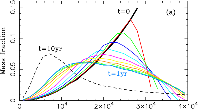
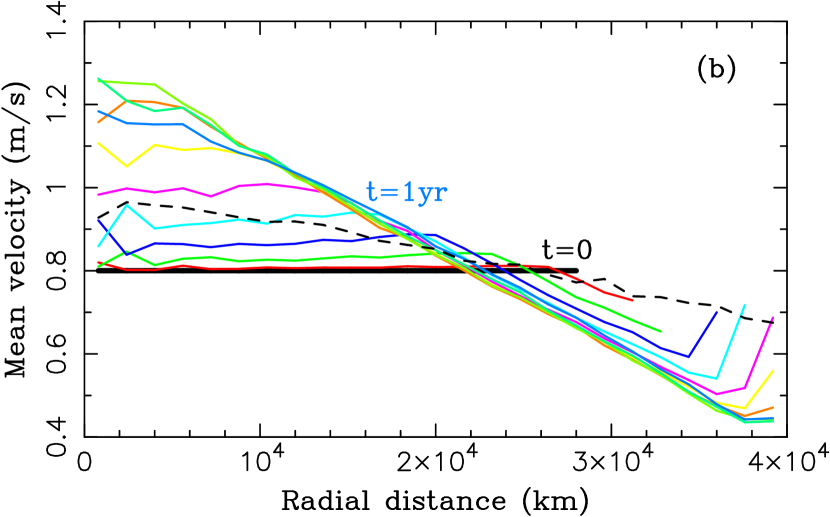
Figure 1: The mass (a) and mean velocity (b) profiles of a self-gravitating collisional cloud. Initially, $10^{6}$ particles with $r\simeq 35$ km were homogeneously distributed in a spherical volume with $f_{\rm H}=0.1$, $a=45$ au and $v_{\rm rand}=0.8$ m s^-1. Here we used $C_{\rm R}=1$ (fully elastic case). The solid and dashed lines show the initial ($t=0$) and final ($t=10$ yr) profiles. The colored lines follow profiles at 0.1 yr increments from $t=0$ to 1 yr.

Figure 1a shows the radial mass distribution of the cloud. We divided the integration domain, represented by a sphere of radius 40,000 km, into 25 concentric shells of equal radial width, ${\rm d}{\cal R}$, and plot the mass in each shell as a fraction of the total mass ($M\simeq 5\times 10^{20}$ g). Mathematically, the plotted quantity is ${\rm d}M({\cal R})/M=4\pi\rho{\cal R}^{2}{\rm d}{\cal R}/M$, where $\rho$ is the mass density at radius ${\cal R}$. For the singular isothermal profile with $\rho\propto{\cal R}^{-2}$ (Binney & Tremaine 1987), ${\rm d}M({\cal R})=$ const. Thus our mass profiles highlight differences relative to $\rho\propto{\cal R}^{-2}$.

By design most mass is initially contained in the radial shells near the outer edge of the cloud. Over one free fall timescale the cloud contracts and the radial mass distribution has a maximum near 15,000 km. This trend continues during the subsequent evolution until eventually, by the end of the simulation, the maximum mass fraction is near 7,000 km. This is a by-product of particle inflation. The total volume of the inflated particles is equivalent to a sphere of radius $\simeq$3,500 km. Thus, as the cloud contracts, the center becomes crowded and the mass of the inner shells cannot increase beyond certain limits. The final profile in the outer regions approaches a theoretical profile of the isothermal sphere, where our mass distribution is expected to be independent of the radial distance (Binney & Tremaine 1987; their Eq. 4-123).

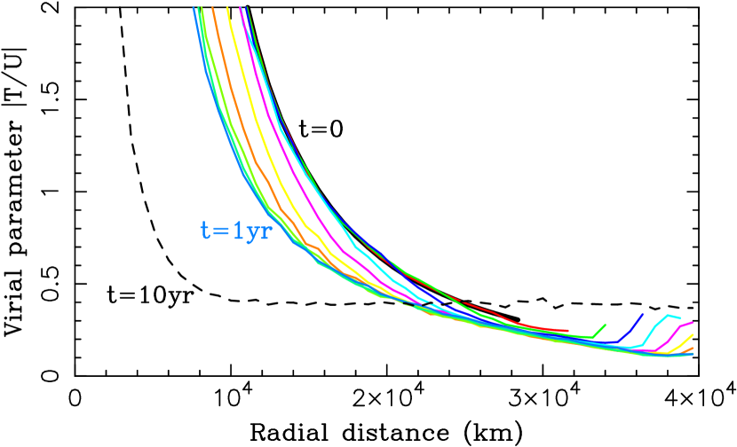
Figure 2: The ratio of kinetic ($T$) and potential ($U$) energies as a function of radial distance. The line styles and parameters used here are the same as in Fig. 1. The potential energy was computed as $U=-GM({\cal R})/{\cal R}$, where $M({\cal R})$ is the mass of particles inside a sphere of radius ${\cal R}$.

Whereas this kind of behavior of radial profiles and velocity distributions is not predicted by the simple arguments in Section 2, the collapse timescale is roughly that of the free fall given by Eq. (10). Recall that the simulated particles were initially given random velocities $v_{\rm rand}=0.8$ m s^-1. The velocities increase in the inner region during the free fall stage (Fig. 1b). After that, collisions act to virialize the system and the radial velocity profiles become flatter (dashed line in Fig. 1b). Eventually, the whole cloud, except for its crowded inner region, evolves toward the virial equilibrium at each radius (Fig. 2). The slightly sub-virial conditions in the outer region ($T/|U|\simeq 0.4$ for $t=10$ yr; Fig. 2) can be explained if particles are preferentially located near their orbital apocenters.

Additional simulations were performed with the SP method described in Section 3. To start with, we used $10^{3}$ SPs each representing $n=10^{3}$ RPs. The simulations were done in the elastic regime and were thus not meant to test Eq. (13). The total energy change and departure from the virial equilibrium were both found to be slightly larger than in the fiducial case, probably due to the increased graininess of particle interactions. We also monitored the behavior of the SP system to see whether it reproduced Figs. 1 and 2. We found that, indeed, the behavior was very similar and the radial profiles, random velocities and energies closely followed the trends described above. More information on these comparisons is provided below. The results with $10^{4}$ and $10^{5}$ SPs were found to be nearly identical to those obtained with $10^{6}$ RPs. The $10^{2}$ SP case, however, already significantly deviated from the reference case in that it showed a far weaker particle concentration near the center. This happened because SPs were strongly inflated and reached maximum packing in the center well before the collapse was completed.

4.2 Inelastic collisions

The main goal of the tests reported here was to verify whether the SP method described in Section 3 correctly reproduces the energy loss. To this end we adopted $C_{\rm R}<1$ and varied the algorithm by which RPs were assigned to their parent SPs. We considered cases with equal and unequal sizes of RPs. For example, we used a power-law size distribution with $q=3$ and distributed RPs within a factor 4 in size around $r\simeq 35$ km (i.e., the value used in the equal-size case). The most massive RPs thus had 64 times the mass of the least massive RPs. The SP method was tested for power-law distributions with $Q=1$, 2 and 3 (Sect 3.1).

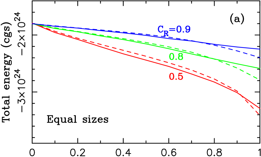
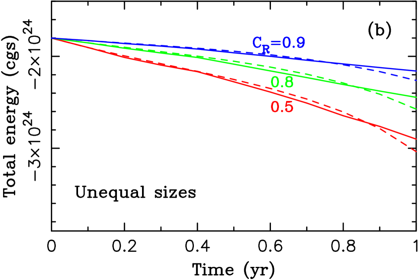
Figure 3: The change of total energy for a case with equal-size particles (panel a) and unequal-size particles (panel b). Different lines correspond to $C_{\rm R}=0.5$ (red), 0.8 (green) and 0.9 (blue). In each case, the solid line shows the result obtained by simulating $10^{6}$ particles. The dashed lines show the results obtained with $10^{3}$ SPs. For the unequal-size case, we used $q=2$ and $Q=1$ (Section 3.1). The results with $Q=2$ and $Q=3$ are nearly identical to the ones shown here for $Q=1$. We were unable to determine the energy loss beyond roughly one free fall timescale, because particles became crowded in the center and the simulations stalled just past $t=1$ yr due to an excessive number of collisions.

We experimented with $C_{\rm R}=0.5$, 0.8 and 0.9. The total energy loss from Eqs. (4) and (5) is expected to be 1.5, 0.7 and 0.4 ($\times 10^{24}$ in cgs units per year; Eq. (6) does not apply, as we discussed in Sect. 2.3, because the collapse happens on the free fall timescale). For comparison, the energy loss in a yr-long interval of the simulation with $10^{6}$ RPs was 1.6, 1 and 0.6 ($\times 10^{24}$ in cgs units), respectively (Fig. 3). This is reasonable. An exact match is not expected because the equations describe an average behavior that doesn’t account for spatial variations (or the time evolution of these variations) in the cloud.

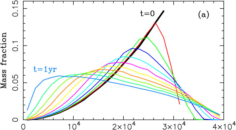
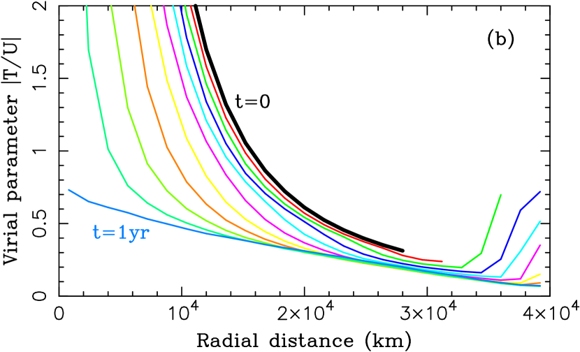
Figure 4: The mass (a) and energy (b) profiles of a self-gravitating collisional cloud of particles. The line styles and simulation parameters used here are the same as in Fig. 1, except in this case $C_{\rm R}=0.5$. The random velocities are damped by inelastic collisions resulting in a stronger particle concentration in the inner region (compare panel (a) with Fig. 1a). The simulation stalls just after $t=1$ yr due to an excessive number of collisions in the inner region.

The superparticle method with $10^{3}$ SPs replicated the energy loss reasonably well (Fig. 3). The small difference between the solid and dashed lines in Fig. 3 is a consequence of a relatively small number of SPs. The results with $10^{4}$ and $10^{5}$ SPs more closely replicated the reference case. The energy loss was more random and a factor of $\sim$2 too small overall with only 100 SPs. We therefore focus on the $10^{3}$ SP case in the following tests, but comment on the results with other sampling rates as well. The radial mass profiles obtained in the case with $C_{\rm R}$=0.5 (maximum dissipation tested here; Fig. 4a) are similar to those obtained in the elastic case (Fig. 1a) except that the particles are even more crowded toward the center, and this trend becomes stronger with time. This is a consequence of the energy loss in inelastic collisions that damp random velocities and facilitate collapse. Eventually, as the number of collisions increased beyond reasonable limits in the central region, the code was unable to make any progress. We stopped all simulations at $t=1$ yr.

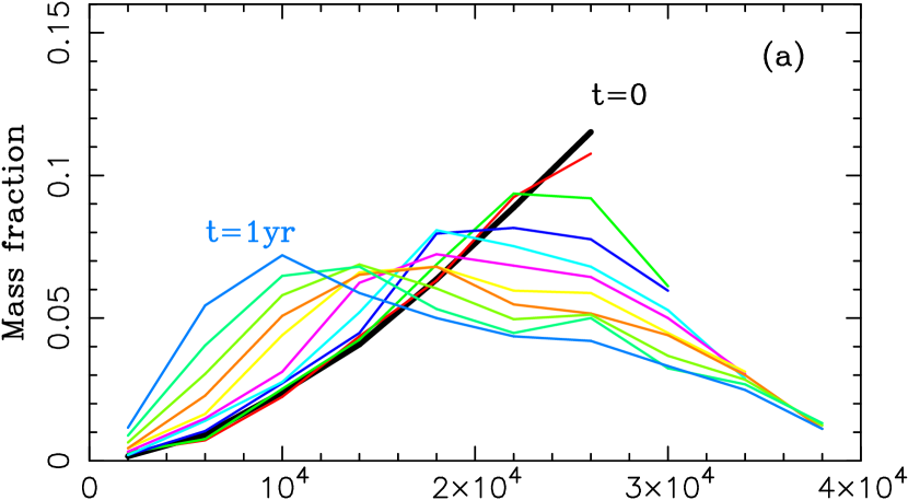
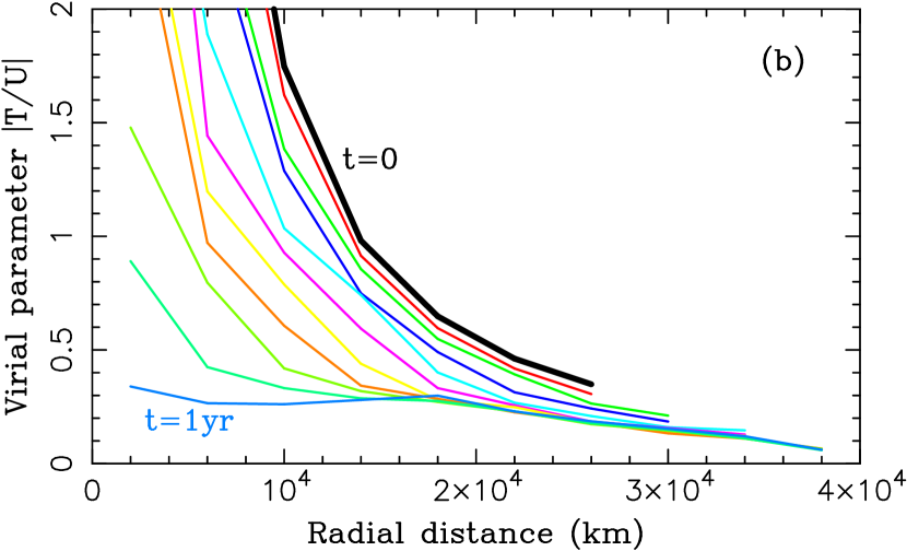
Figure 5: The mass (a) and energy (b) profiles of a self-gravitating collisional cloud. The simulation setup is the same as in Fig. 4, except that here we used $10^{3}$ SPs each representing $n=10^{3}$ RPs. The radial bin size was increased to compensate for poor resolution (10 bins here vs. 25 bins in previous figures). Panel (a) can be compared to Fig. 4a and panel (b) to Fig. 4b.

The virial parameter $T/|U|$ is shown in Fig. 4b. The $T/|U|$ ratio is generally smaller than that in Fig. 2 at least partly because here the kinetic energy decays by dissipative collisions. This becomes especially clear near the center as time approaches the free fall timescale. All these trends are well reproduced with the SP method (Fig. 5). As the SPs occupy a larger volume, however, they are not allowed to concentrate as strongly toward the center as in the reference case. This leads to the mass distribution that peaks at somewhat larger radial distance (compare Fig. 4a and Fig. 5a). This “packing” problem becomes less (more) of an issue with $>10^{3}$ SPs ($<10^{3}$ SPs). In addition, the radial profiles become very noisy with only $10^{2}$ SPs, suggesting that this sampling rate is not adequate to capture the statistical behavior of the real system.

We verified that the total angular momentum $L$ is conserved by adding solid initial rotation of the cloud around the $z$ axis. At the cloud’s outer radius of $\simeq$30,000 km, the circular speed is $v_{\rm circ}=\sqrt{GM/R}\simeq 1.1$ m s^-1. We thus added angular speed $\Omega=f_{\Omega}v_{\rm circ}/R$, where $f_{\Omega}\geq 0$ is a scaling factor. Specifically, for the tests in the following section, we used $f_{\Omega}=0.5$ and $\Omega\simeq 1.7\times 10^{-8}$ s^-1. This choice was motivated by rotation inferred for self-gravitating pebble clouds from our SI simulations (e.g., Nesvorný et al. 2019, Li et al. 2019), but note that the initial structure of SI clouds is generally complex and cannot be idealized by solid rotation of homogeneous spheres. Here we used the idealized case to test the SP method. More realistic initial conditions will be investigated elsewhere. We found that the angular momentum was very well conserved in both the reference case (relative change $\delta L/L\sim 3\times 10^{-6}$) and when the SP method was used (e.g., $\delta L/L\sim 5\times 10^{-5}$ for the case with $10^{3}$ SPs).

4.3 Mergers

Here we tested the merger algorithm described in Section 3.3. The general setup of the simulations was the same as the one used above. We tested cases with ($f_{\Omega}=0.5$) and without ($f_{\Omega}=0$) cloud rotation. The initial rotation provides centrifugal support to the cloud and reduces problems with particle crowding. We found that the case with $f_{\Omega}=0.5$ is more suitable for comparisons than $f_{\Omega}=0$ because the results are less sensitive to various integration details (e.g., the seed used to generate the initial conditions). The results for $f_{\Omega}=0$ are reported below for completeness. In PKDGRAV, particle mergers are applied if the collision speed between particles $v_{\rm col}<f_{\rm esc}v_{\rm esc}$, where $v_{\rm esc}$ is the escape speed and $f_{\rm esc}<1$ is a free parameter. Collisions with $v_{\rm col}>f_{\rm esc}v_{\rm esc}$ result is particle bounces.

Figure 6 shows the size distributions obtained in the simulations with $10^{6}$ RPs and $10^{3}$ SPs. In both cases, we used $v_{\rm rand}=0.8$ m s^-1, $C_{\rm R}=0.5$, $f_{\Omega}=0$ and $f_{\rm esc}=0.1$. In the reference case, we simply plot the size distribution of RPs. In the SP simulation, the size distribution is constructed from the number and sizes of particles represented by each SP. We found that the SP algorithm with $10^{3}$ SPs can reproduce the particle growth quite well but the results had a rather large statistical variability with minor changes of the input (e.g., when different seeds were used to generate initial conditions). We interpret this as a consequence of stochastic interaction of large bodies that grow in the center of the collapsing cloud. The stochasticity of the results diminishes if $>10^{3}$ SPs are used. For this reason, in the rest of this section, we discuss the results obtained with $f_{\Omega}=0.5$, as rotation inhibits collapse to the center of mass. For reference, the radii of the largest bodies shown in Fig. 6 are $\simeq$3200 km (panel a) and $\simeq$2500 km (panel b).

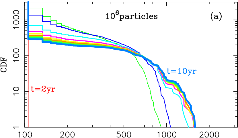
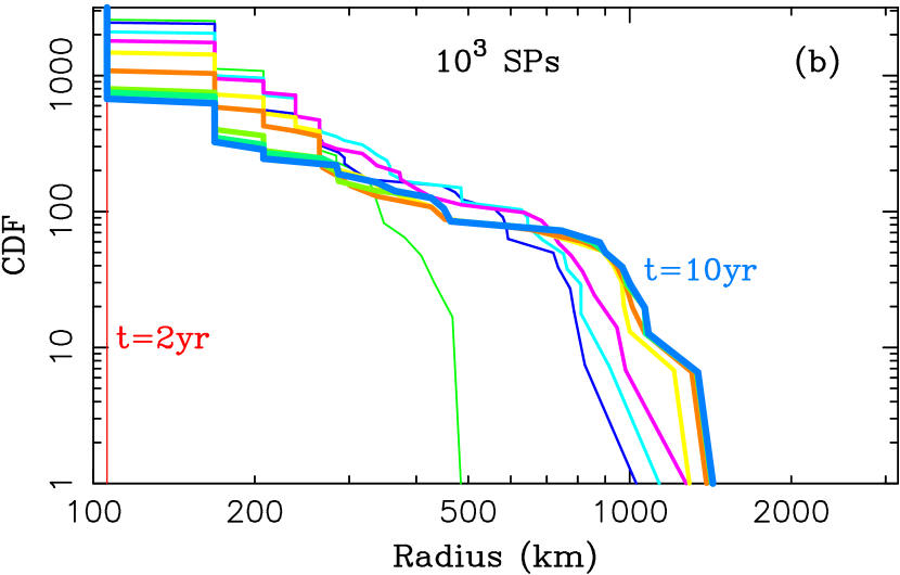
Figure 7: The cumulative size distributions of particles for the case with $C_{\rm R}=0.5$ and $f_{\Omega}=0.5$. See caption of Fig. 6 for additional information.

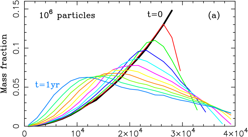
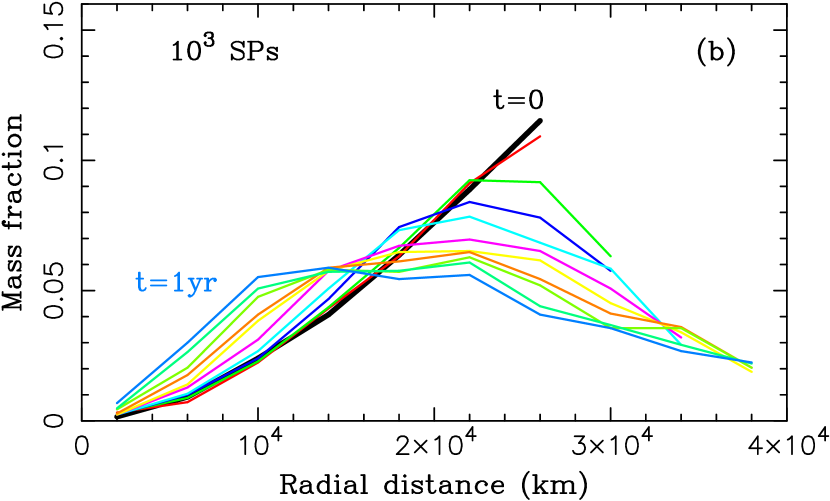
Figure 8: The radial profiles for the case in Fig. 7. The profiles are shown for $0<t<1$ yr in 0.1 yr increments. The profiles become noisy for $t>1$ yr (not shown here) when large bodies grow in the cloud. Panels (a) and (b) show the cases with $10^{6}$ particles and $10^{3}$ SPs, respectively.

The case with $f_{\Omega}=0.5$ does not produce bodies that are as large (Fig. 7). The largest objects have the radii $\simeq$1600 km (panel a; $10^{6}$ RPs) and $\simeq$1400 km (panel b; $10^{3}$ SPs). Both simulations ended with a rounded cumulative distribution function (CDF) profile and dozens of bodies larger than 1000 km. For $f_{\Omega}=0.5$, the SP method somewhat overshoots the number of the smallest objects but the difference is not large (the case with $f_{\Omega}=0$ produced an opposite result; Fig. 6). We repeated the SP simulations with slightly changed initial conditions and found that the results were quite similar to those shown in Fig. 7b. This means that the stochastic variations are not as large for $f_{\Omega}=0.5$ as they were for $f_{\Omega}=0$. The radial mass distribution profiles are compared in Fig. 8. The SP method with $10^{3}$ SPs reasonably well replicates the profiles obtained in the fiducial case. The results with $10^{4}$ and $10^{5}$ SPs reproduce the fiducial radial profiles and size distributions even more closely.

Figure 9 shows the evolving structure of the particle cloud with $f_{\Omega}=0.5$. First, an agglomerate of particles formed in the center. The agglomerate had significant rotation and stretched along one direction to a $\simeq$7:1 axial ratio. Then, roughly at $t=4$ yr, the extremes detached to release the angular momentum whereas the middle part of the agglomerate remained connected. Several small binaries formed at this point. Eventually, when the simulation was extended to $t=100$ yr, a massive, equal-size binary formed in the center. The two components of the binary had radii $R_{1}=24.1$ km and $R_{2}=20.5$ km and a separation of $a_{\rm B}=4530$ km. Thus $a_{\rm B}/(R_{1}^{3}+R_{2}^{3})^{1/3}\simeq 160$, which is quite typical for the equal-size binaries in the trans-Neptunian region (Grundy et al. 2019, Nesvorný & Vokrouhlický 2019). The total mass of the binary object represents 18% of the initial cloud’s mass. This suggests that planetesimal masses estimated from the total cloud mass (e.g., Simon et al. 2017) could be overestimated by an order of magnitude.

5 Conclusions

We developed a new method that will be useful for modeling statistically large collisional systems of particles. The method represents a significant computational speed-up by employing far fewer “superparticles” than the number of particles in the real system. It reproduces the energy loss in dissipative collisions of real particles and can account for particle growth by mergers. We implemented the method in the PKDGRAV code and tested it. We found that at least $\sim$$10^{3}$ superparticles need to be used to reproduce the results of our fiducial simulations with full resolution. The number of superparticles needed in real-world applications will have to be determined by convergence studies tailored to those applications. As the superparticles need to be inflated to represent a much larger collisional cross-section of the real system, particle crowding may become a problem in some applications. In the gravitational collapse simulation performed here, this becomes apparent near the cloud’s center, where the code has difficulties to account for a vast number of superparticle collisions. This problem can be mitigated by using a larger number of (less-inflated) superparticles, merging superparticles and/or letting PKDGRAV form rigid particle aggregates.

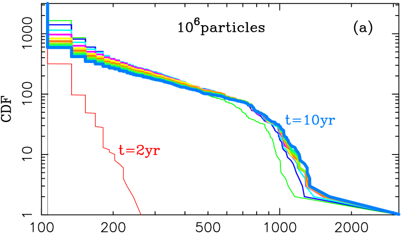
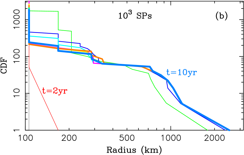
Figure 6: The cumulative size distributions of particles for the case with $C_{\rm R}=0.5$ and $f_{\Omega}=0$. Mergers between particles occur in PKDGRAV when the collision speed is less then 0.1 of the particle escape speed. The size distribution is shown for $0<t<10$ yr in 1 yr increments (from thin black to thick blue lines). The reference case with $10^{6}$ particles is shown in panel (a). The case with $10^{3}$ SPs is shown in panel (b).

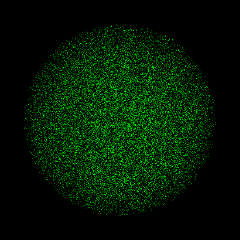
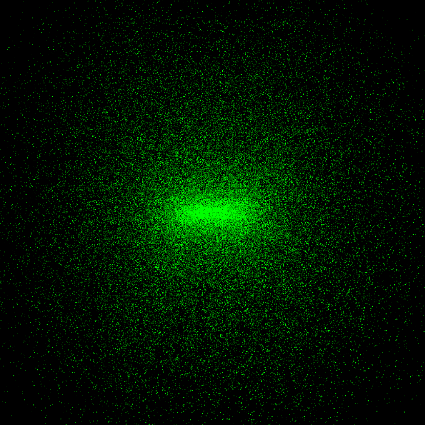
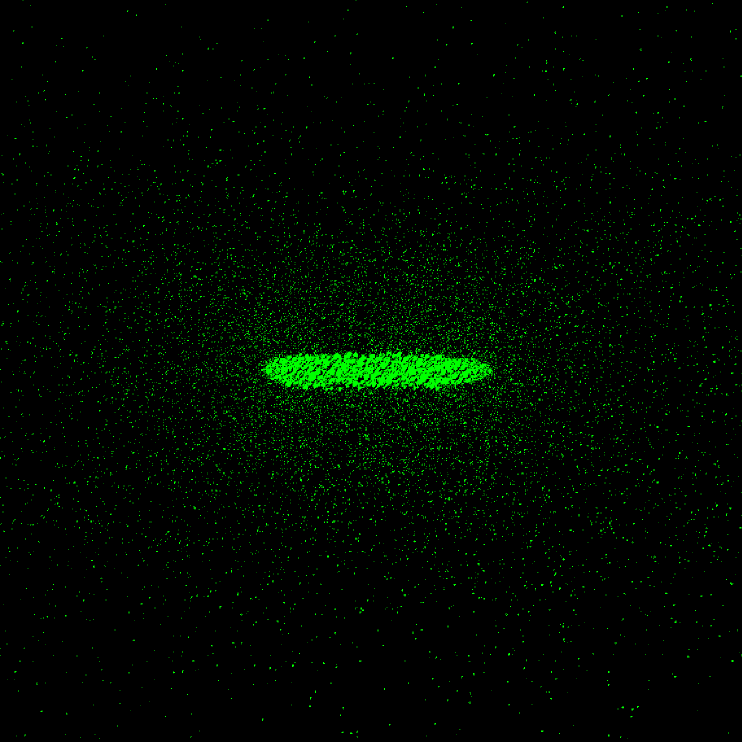
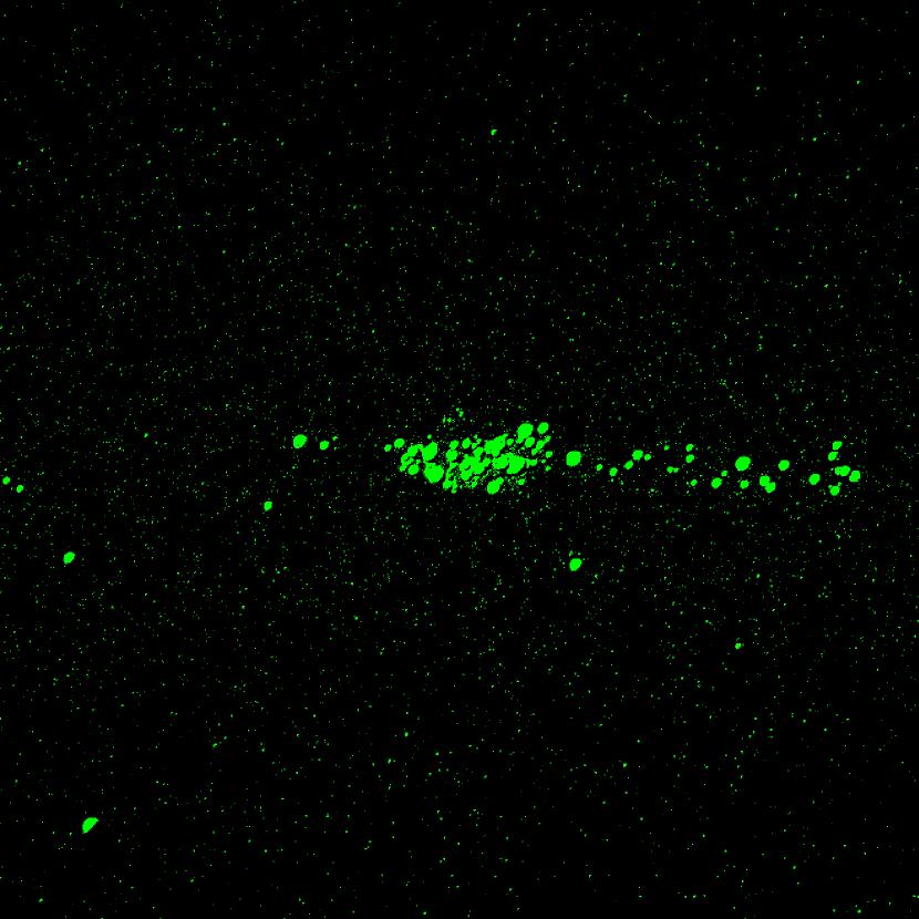
Figure 9: Four snapshots showing particle distributions at $t=0$ (top left), 1.2 (top right), 3 (bottom left) and 7 years (bottom right). This is for the case with $C_{\rm R}=0.5$ and $f_{\Omega}=0.5$.

References

- Bai,& Stone (2010) Bai, X.-N., & Stone, J. M. 2010, ApJS, 190, 297
- Binney & Tremaine (1987) Binney, J., & Tremaine, S. 1987, Princeton
- Birnstiel et al. (2016) Birnstiel, T., Fang, M., & Johansen, A. 2016, Space Sci. Rev., 205, 41
- Bai, & Stone (2011) Grundy, W. M., Noll, K. S., Roe, H. G. et al. 2019, Icarus, 334, 62
- Chiang & Youdin (2010) Chiang, E., & Youdin, A. N. 2010, Annual Review of Earth and Planetary Sciences, 38, 493
- Johansen & Youdin (2007) Johansen, A., & Youdin, A. 2007, ApJ, 662, 627
- Johansen et al. (2009) Johansen, A., Youdin, A., & Mac Low, M. 2009, ApJ, 704, L75
- Johansen et al. (2014) Johansen, A., Blum, J., Tanaka, H., et al. 2014, Protostars and Planets VI, 547
- Li et al. (2019) Li, R., Youdin, A. N., & Simon, J. B. 2019, ApJ, 885, 69
- Michikoshi & Kokubo (2016) Michikoshi, S., & Kokubo, E. 2016, ApJ, 825, L28
- Nesvorný et al. (2010) Nesvorný, D., Youdin, A. N., & Richardson, D. C. 2010, AJ, 140, 78 5 (NYR10)
- Nesvorný et al. (2019) Nesvorný, D., Li, R., Youdin, A. N., Simon, J. B., & Grundy, W. M. 2019, Nature Astronomy
- Nesvorný, & Vokrouhlický (2019) Nesvorný, D., & Vokrouhlický, D. 2019, Icarus, 331, 49
- Richardson et al. (2000) Richardson, D. C., Quinn, T., Stadel, J., et al. 2000, Icarus, 143, 45
- Simon et al. (2017) Simon, J. B., Armitage, P. J., Youdin, A. N., et al. 2017, ApJ, 847, L12
- Stadel (2001) Stadel, J. G. 2001, Ph.D. Thesis
- Wahlberg Jansson, & Johansen (2014) Wahlberg Jansson, K., & Johansen, A. 2014, A&A, 570, A47
- Wahlberg Jansson et al. (2017) Wahlberg Jansson, K., Johansen, A., Bukhari Syed, M., et al. 2017, ApJ, 835, 109
- Youdin, & Goodman (2005) Youdin, A. N., & Goodman, J. 2005, ApJ, 620, 459
- Youdin & Johansen (2007) Youdin, A., & Johansen, A. 2007, ApJ, 662, 613
- Youdin & Kenyon (2013) Youdin, A. N., & Kenyon, S. J. 2013, Planets, Stars and Stellar Systems. Volume 3: Solar and Stellar Planetary Systems, 1