Abstract

We use Noether symmetry approach to find spherically symmetric static solutions of the non-minimally coupled electromagnetic fields to gravity. We construct the point-like Lagrangian under the spherical symmetry assumption. Then we determine Noether symmetry and the corresponding conserved charge. We derive Euler-Lagrange equations from this point-like Lagrangian and show that these equations are same with the differential equations derived from the field equations of the model. Also we give two new exact asymptotically flat solutions to these equations and investigate some thermodynamic properties of these black holes.

I Introduction

The late time expansion of the universe and the missing matter at large astrophysical scales still remain the most important issues of modern cosmology. Although Einstein’s gravity with the cosmological constant known as $\Lambda$CDM is in agreement with the observations, it has some problems such as fine tuning and coincidence. Since dark matter particle has not yet been observed directly, the efforts to modify the Einstein’s theory of gravity have recently increased by studying the models such as $f(R)$ gravity, scalar-tensor gravity and vector-tensor gravity.

Due to the modification of the Einstein’s gravity, it is possible to modify the Einstein-Maxwell theory to the $f(R)$-Maxwell theory in the presence of the electromagnetic field. The spherically symmetric static solution of this theory with constant Ricci scalar, which is similar to the Reissner-Nordstrom-AdS black hole solution, was given in Dombriz2009 . However, in general cases with dynamical non-constant Ricci scalar, it is not easy to find more general solutions. Then one can take into account the non-minimal couplings between electromagnetic fields and gravity like $Y(R)F^{2}$-type. The feature of the non-minimal theory is to have a large class of solutions such as the spherically symmetric DereliSert20111 ; DereliSert20112 ; Sert2012Plus ; Sert2013MPLA ; Sert2016regular and cosmological solutions AADS ; Sert2019 ; SertAdak2019 . It is interesting to note that such non-minimal couplings, which are first order in R, have been obtained in MullerHoissen19882 ; MullerHoissen19883 ; Buchdahl1979 ; Dereli1990 from a five-dimensional Lagrangian via dimensional reduction. Also, Prasanna1971 ; Horndeski1976 ; MullerHoissen1988 ; Drummond1980 investigated various aspects of these couplings, such as charge conservation and the relationship between electric charge and geometry. The general couplings in $R^{n}F^{2}$-form applied to the generation of primordial magnetic fields in the inflation stage Turner1988 ; Campanelli2008 ; Kunze2010 ; Mazzi1995 ; AADS ; Sert2019 ; Bamba2008 . Therefore, it is possible to consider the more general couplings in $Y(R)F^{2}$ form and their solutions can give us more information about the relation between electric charge and space-time curvature. Especially in the presence of medium with very high density electromagnetic fields, these couplings may arise and their effects can be significant even far from the source.

The Noether symmetry approach is one of the effective techniques to find solutions of a Lagrangian without using field equations. This symmetry approach allows us to find conserved quantities of a model by using the symmetry of the Lagrangian which is invariant along a vector field. Then the vector field can be determined by this symmetry and each symmetry of the Lagrangian gives a conserved quantity. This symmetry approach has been applied to $f(R)$ gravity successfully to find out solutions and select the corresponding $f(R)$ function which is compatible with the Noether symmetry Capozziello2007 ; Capozziello2000 ; Capozziello2008 .

This study is organized as follows: In the second section, we find the first order point-like action of the model for the spherically symmetric static metric and electric field. After we apply the Noether symmetry approach to the action, we obtain the system of partial differential equations. By solving the system, we find the Noether charge and the corresponding vector field for the non-minimal $Y(R)F^{2}$ model. In the third section, after we obtain Euler-Lagrange equations we give two new solutions to the equations and investigate some thermodynamic properties of the black hole solutions. Finally, we summarize the results in the last section.

II Noether Symmetry Approach for the Non-Minimal Model

Let us start with the following action of the non-minimally coupled electromagnetic fields to gravity DereliSert20111 ; DereliSert20112 ; Bamba2008

$$\mathcal{I}=\int\ \left[\frac{R}{2\kappa^{2}}*1-Y(R)F\wedge*F\right].$$ (1)

By taking the variation of the action, and obtaining the field equations, we can find the solutions DereliSert20111 ; DereliSert20112 ; Sert2012Plus ; Sert2013MPLA ; Sert2016regular for the spherically symmetric static metric

$$ds^{2}=-A(r)dt^{2}+\frac{1}{A(r)}dr^{2}+B(r)d\theta^{2}+B(r)\sin^{2}\theta d\varphi^{2}\ .$$ (2)

Here the corresponding Ricci curvature scalar is

$$R=-A^{\prime\prime}-\frac{2AB^{\prime\prime}}{B}-\frac{2A^{\prime}B^{\prime}}{B}+\frac{AB^{\prime 2}}{2B^{2}}+\frac{2}{B}\ .$$ (3)

Alternatively, we can find the solutions also from Noether symmetry approach by taking the following action of the non-minimally coupled model with the Lagrange multiplier $\lambda$

$$\mathcal{I}=\int\ \left[\frac{R}{2\kappa^{2}}*1-Y(R)F\wedge*F-\ \lambda(R-\bar{R})*1\right].$$ (4)

Here variation of the action with respect to $\lambda$ gives us $R=\bar{R}$ and $\bar{R}$ is defined as

$$\bar{R}=R^{*}-A^{\prime\prime}-\frac{2AB^{\prime\prime}}{B}$$ (5)

to eliminate the second order derivatives in the action via integration by parts. Here $R^{*}$ is defined as $R^{*}=-\frac{2A^{\prime}B^{\prime}}{B}+\frac{AB^{\prime 2}}{2B^{2}}+\frac{2}{B}\;.$ The variation of the action with respect to $R$ gives

$$\lambda=\frac{1}{2\kappa^{2}}*1-Y_{R}(R)F\wedge*F\$$ (6)

where $Y_{R}(R)=\derivative{Y(R)}{R}$. If we substitute (5) and (6) in the action (4), we obtain the following Lagrangian

$$L = \frac{R}{2\kappa^{2}}*1-Y(R)F\wedge*F-\left(\frac{1}{2\kappa^{2}}*1-Y_{R}(R)F\wedge*F\right)\left(R-R^{*}+A^{\prime\prime}+\frac{2AB^{\prime\prime}}{B}\right)\ .$$ (7)

We see that $Y_{R}(R)F\wedge*F$ term in the Lagrangian has higher order derivatives which complicates the Noether approach. But, fortunately we have the following equation from the trace of the field equations

$$Y_{R}(R)F\wedge*F=-\frac{1}{2\kappa^{2}}$$ (8)

which corresponds to the conservation of the energy-momentum tensor Sert2019 and eliminates the higher order derivatives in the Lagrangian. By taking the electromagnetic tensor $F$,

$$F=\phi^{\prime}(r)e^{1}\ \wedge e^{0}\;,$$ (9)

which has only the electric potential $\phi(r)$, the Lagrangian of the model is obtained as

$$L = \frac{B}{\kappa^{2}}\left[-\frac{R}{2}+\kappa^{2}Y(R)\phi^{\prime 2}+R^{*}-A^{\prime\prime}-\frac{2AB^{\prime\prime}}{B}\right]\;.$$ (10)

In the Lagrangian, the second order derivatives can be eliminated by integration by parts and it turns out to be the following point-like Lagrangian

$$L=\frac{AB^{\prime 2}}{2\kappa^{2}B}+\frac{A^{\prime}B^{\prime}}{\kappa^{2}}-\frac{BR}{2\kappa^{2}}+BY(R)\phi^{\prime 2}+\frac{2}{\kappa^{2}}\;.$$ (11)

By considering the the configuration space $Q$ which has the generalized coordinates $q^{i}\equiv\{A,B,\phi,R\}$ and its tangent space $TQ\equiv\{q^{i},q^{\prime i}\}$, we look for the symmetries of the Lagrangian. Noether’s theorem states that if the Lie derivative of a Lagrangian vanishes

$$\mathcal{L}_{X}L(q^{i},q^{\prime i})=XL(q^{i},q^{\prime i})=0$$ (12)

along a vector field $X$

$$X=\alpha_{i}\frac{\partial}{\partial q^{i}}+\alpha^{\prime}_{i}\frac{\partial}{\partial q^{\prime i}},$$ (13)

then $X$ is a symmetry of the action and each symmetry of the action corresponds to a conserved quantity or first integral such as

$$\Sigma_{0}=\alpha_{i}\frac{\partial L}{\partial q^{\prime i}}\;.$$ (14)

Then we take the Lie derivative of the point-like Lagrangian in the configuration space to find the first integral

$$\mathcal{L}_{X}L = \alpha_{1}\frac{\partial L}{\partial A}+\alpha_{2}\frac{\partial L}{\partial B}+\alpha_{3}\frac{\partial L}{\partial\phi}+\alpha_{4}\frac{\partial L}{\partial R}$$ (16)

$$+\alpha_{1}^{\prime}\frac{\partial L}{\partial A^{\prime}}+\alpha_{2}^{\prime}\frac{\partial L}{\partial B^{\prime}}+\alpha_{3}^{\prime}\frac{\partial L}{\partial\phi^{\prime}}+\alpha_{4}^{\prime}\frac{\partial L}{\partial R^{\prime}}$$

$$= \alpha_{1}\frac{B^{\prime 2}}{2\kappa^{2}B}+\alpha_{2}\left(\frac{-AB^{\prime 2}}{2\kappa^{2}B^{2}}-\frac{R}{2\kappa^{2}}+Y(R)\phi^{\prime 2}\right)$$

$$+\alpha_{4}\left(\frac{-B}{2\kappa^{2}}+BY_{R}(R)\phi^{\prime 2}\right)+\alpha_{1}^{\prime}\frac{B^{\prime}}{\kappa^{2}}+\alpha_{2}^{\prime}\left(\frac{AB^{\prime}}{\kappa^{2}B}+\frac{A^{\prime}}{\kappa^{2}}\right)$$

$$+\alpha_{3}^{\prime}2BY(R)\phi^{\prime}=0$$

where $\alpha_{i}=\alpha_{i}(A,B,\phi,R)$. Here the derivatives $\alpha_{i}^{\prime}$ can be written by the chain rule

$$\alpha_{i}^{\prime}=\frac{\partial\alpha_{i}}{\partial A}A^{\prime}+\frac{\partial\alpha_{i}}{\partial B}B^{\prime}+\frac{\partial\alpha_{i}}{\partial\phi}\phi^{\prime}+\frac{\partial\alpha_{i}}{\partial R}R^{\prime}$$ (17)

and the Lie derivative of the point-like Lagrangian gives us the following system of partial differential equations

$$\frac{\alpha_{1}}{2B}-\frac{\alpha_{2}A}{2B^{2}}+\frac{\partial\alpha_{1}}{\partial B}+\frac{\partial\alpha_{2}}{\partial B}\frac{A}{B} = 0,$$ (18)

$$\alpha_{2}Y(R)+\alpha_{4}BY_{R}(R)+2\frac{\partial\alpha_{3}}{\partial\phi}BY(R) = 0,$$ (19)

$$\frac{\partial\alpha_{1}}{\partial\phi}\frac{1}{\kappa^{2}}+\frac{\partial\alpha_{2}}{\partial\phi}\frac{1}{\kappa^{2}}\frac{A}{B}+2\frac{\partial\alpha_{3}}{\partial B}BY(R) = 0,$$ (20)

$$\frac{\partial\alpha_{1}}{\partial A}+\frac{\partial\alpha_{2}}{\partial A}\frac{A}{B}+\frac{\partial\alpha_{2}}{\partial B} = 0,$$ (21)

$$\frac{\partial\alpha_{2}}{\partial\phi}\frac{1}{\kappa^{2}}+2\frac{\partial\alpha_{3}}{\partial A}BY(R) = 0,$$ (22)

$$\frac{\partial\alpha_{1}}{\partial R}+\frac{\partial\alpha_{2}}{\partial R}\frac{A}{B} = 0,$$ (23)

$$\frac{\partial\alpha_{2}}{\partial A}=0,\hskip 14.22636pt\frac{\partial\alpha_{2}}{\partial R}=0,\hskip 14.22636pt\frac{\partial\alpha_{3}}{\partial R}BY(R) = 0,$$ (24)

$$\alpha_{2}R+\alpha_{4}B = 0.$$ (25)

A solution to the system for an arbitrary $Y(R)$ function can be found as

$$\alpha_{1}=\frac{c_{1}}{\sqrt{B}},\hskip 14.22636pt\alpha_{2}=0,\hskip 14.22636pt\alpha_{3}=c_{2},\hskip 14.22636pt\alpha_{4}=0\;.$$ (26)

Here $c_{1},c_{2}$ are arbitrary constants. Then the $X$ vector field can be found as

$$X=\frac{c_{1}}{\sqrt{B}}\frac{\partial}{\partial A}-\frac{c_{1}}{2B^{3/2}}\frac{\partial}{\partial A^{\prime}}+c_{2}\frac{\partial}{\partial\phi}\$$ (27)

and the the constant of motion (14) becomes

$$\Sigma_{0}=\frac{2c_{1}}{\kappa^{2}}+2c_{2}BY(R)\phi^{\prime}\ .$$ (28)

III Euler-Lagrange equations

In order to determine the non-minimal function and the metric functions, we calculate the Euler-Lagrange equations from

$$\frac{d}{dr}(\frac{\partial L}{\partial q^{\prime i}})-\frac{\partial L}{\partial q^{i}}=0$$ (29)

for the Lagrangian (11). Then we obtain the following differential equations for $A,B,\phi,R$, respectively:

$$B^{\prime\prime}-\frac{B^{\prime 2}}{2B}=0,$$ (30)

$$\frac{A^{\prime}B^{\prime}}{B}+\frac{AB^{\prime\prime}}{B}-\frac{AB^{\prime 2}}{2B^{2}}+A^{\prime\prime}+\frac{R}{2}-Y(R)\phi^{\prime 2}\kappa^{2}=0,$$ (31)

$$(B\phi^{\prime}Y(R))^{\prime}=0,$$ (32)

$$Y_{R}(R)\phi^{\prime 2}=\frac{1}{2\kappa^{2}}\ .$$ (33)

From (30) and (32) we find

$$B(r)=b_{1}(r+b_{2})^{2},\hskip 28.45274ptY(R)\phi^{\prime}=\frac{q}{B},$$ (34)

where $q$ is an integration constant and it corresponds to the electric charge of the source. We note that the condition (33) can be found by taking the derivative of equation (31) with respect to $r$ as in Sert2016regular . Then we have only the following differential equation (31) to solve

$$\frac{A^{\prime\prime}}{2}-\frac{AB^{\prime 2}}{4B^{2}}+\frac{1}{B}-\kappa^{2}Y(R)\phi^{\prime 2}=0$$ (35)

which is same with the differential equation obtained from the field equations of the model in DereliSert20112 ; Sert2012Plus ; Sert2013MPLA ; Sert2016regular for $B=r^{2}$. Thus we show that these two different methods give the same differential equation (35). The conserved charge (28) of the model turns out to be

$$\Sigma_{0}=\frac{2c_{1}}{\kappa^{2}}+2qc_{2}\;$$ (36)

for the Noether symmetry. We see that the conserved quantity involves the gravitational coupling constant $\kappa^{2}$ and the electric charge of the system $q$. We also calculate the energy function from

$$E_{L}=q^{\prime i}(\frac{\partial L}{\partial q^{i}})-L$$ (37)

and find

$$E_{L}=\frac{BR}{2\kappa^{2}}+\frac{AB^{\prime 2}}{2\kappa^{2}B}+\frac{A^{\prime}B^{\prime}}{\kappa^{2}}+BY(R)\phi^{\prime 2}-\frac{2}{\kappa^{2}}\ .$$ (38)

By substituting the Ricci scalar (3) in the energy function (38), we find that the function is equal to zero, since equation (38) is nothing more than equation (35). Furthermore, we can choose $B=r^{2}$ without loss of generality then (35) becomes

$$\frac{A^{\prime\prime}}{2}+\frac{1-A}{r^{2}}-\kappa^{2}Y(R)\phi^{\prime 2}=0\ .$$ (39)

III.1 Some New Solutions

In order to obtain solutions of the differential equation (39), we can choose the non-minimal function $Y(R)$ that determines the strength of the coupling and find the metric function $A(r)$ as a first method. Alternatively, we can choose possible geometries which are asymptotically flat and involve correction terms to the known Reissner-Nordstrom solution as a second method. Then we can find the corresponding non-minimal function $Y(R)$. Here we consider the second method and we take the following metric function with the Yukawa-like correction term

$$A_{1}(r)=1-\frac{2M}{r}+\frac{q^{2}}{r^{2}}-a\frac{e^{-r}}{r^{2}}$$ (40)

which gives the solution

$$\phi(r) = \frac{q}{r}-\frac{ae^{-r}(r+4)}{qr}\;,$$ (41)

$$Y(r) = \frac{8q^{2}/\kappa^{2}}{4q^{2}-a(r+2)^{2}e^{-r}}\;.$$ (42)

Then the Ricci scalar becomes $R=\frac{a}{e^{r}r^{2}}$ for the metric function and by taking the inverse function $r=2W(x)$, we can re-express the non-minimal function (42) in terms of $R$ as

$$Y(R)=\frac{8q^{2}/\kappa^{2}}{4q^{2}-4(W(x)+1)^{2}e^{-2W(x)}}$$ (43)

where $W(x)$ is the Lambert function with $x=\sqrt{\frac{a}{4R}}$.

Secondly, we choose another metric function with the Yukawa-like correction term

$$A_{2}(r)=1-\frac{2M}{r}+\frac{q^{2}}{r^{2}}-(1+\frac{4}{r}+\frac{6}{r^{2}})ae^{-r}$$ (44)

which is also asymptotically flat. Then we obtain the following solution

$$\phi(r) = \frac{q}{r}-\frac{a(r^{3}+6r^{2}+18r+24)e^{-r}}{qr}\;,$$ (45)

$$Y(r) = \frac{8q^{2}/\kappa^{2}}{4q^{2}-a(r^{4}+4r^{3}+12r^{2}+24r+24)e^{-r}}\ .$$ (46)

We calculate the Ricci scalar for the second metric as $R=ae^{-r}$ and the inverse function $r=lnx$ with $x=\frac{a}{R}$. Then the non-minimal function becomes

$$Y(R)=\frac{8q^{2}/\kappa^{2}}{4q^{2}-(ln^{4}x+4ln^{3}x+12ln^{2}x+24lnx+24)R}\ \ .$$ (47)

III.2 Some Thermodynamic Properties of the Solutions

The above metric functions (40) and (44) may describe a naked singularity without horizon or a black hole with one horizon or two horizons which are called event horizon and Cauchy horizon depending on the choice of the parameters. In the cases with event horizon $r=r_{h}$, the Hawking temperature is defined by

$$T=\frac{A^{\prime}(r_{h})}{4\pi}$$ (48)

and the temperatures can be found

$$4\pi T_{1} = \frac{a(r_{h}+2)}{r_{h}^{3}e^{r_{h}}}+\frac{2M}{r_{h}^{2}}-\frac{2q^{2}}{r_{h}^{3}}\;,$$ (49)

$$4\pi T_{2} = \frac{a(r_{h}^{3}+4r_{h}^{2}+10r_{h}+12)}{r_{h}^{3}e^{r_{h}}})+\frac{2M}{r_{h}^{2}}-\frac{2q^{2}}{r_{h}^{3}}\;$$ (50)

for the above metric functions (40) and (44). We give the variation of the temperatures with the event horizon radius $r_{h}$ in Fig. 1 for this non-minimal model and the Reissner-Nordstrom case.

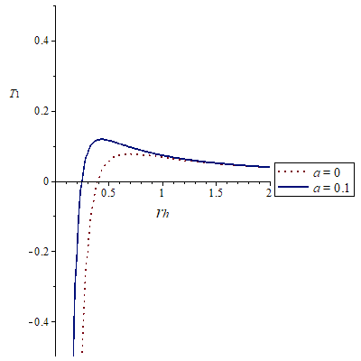
(a)

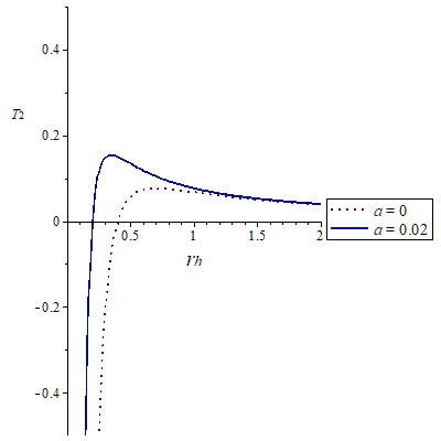
(b)

Figure 1: The Hawking temperature versus the event horizon radius with $q=0.4$, the dotted curve is the Reissner-Nordstrom case and the solid curve is the non-minimal model.

By using the entropy of black hole $S=\pi r_{h}^{2}$, we calculate the heat capacity from

$$C=T\left(\frac{\partial S}{\partial T}\right)_{q}$$ (51)

for the above two metric functions and obtain

$$C_{1} = \frac{2\pi r_{h}^{2}\left((r_{h}^{2}-q^{2})e^{r_{h}}+a(r_{h}+1)\right)}{(3q^{2}-r_{h}^{2})e^{r_{h}}-a(r_{h}^{2}+3r_{h}+3)}\;,$$ (52)

$$C_{2} = \frac{2\pi r_{h}^{2}\left((r_{h}^{2}-q^{2})e^{r_{h}}+a(r_{h}^{3}+3r_{h}^{2}+6r_{h}+6)\right)}{(3q^{2}-r_{h}^{2})e^{r_{h}}-a(r_{h}^{4}+3r_{h}^{3}+9r_{h}^{2}+18r_{h}+18)}\;.$$ (53)

Heat capacity gives us information about thermal stability intervals and phase transition points of a black hole. Heat capacity must be positive and finite for a stable black hole. The points where heat capacity is zero give us the Type-1 instability and the points where heat capacity diverges give us Type-2 instability points which correspond to the second order phase transition for a black hole. We plot also the heat capacity versus the horizon radius $r_{h}$ for the Reissner-Nordstrom solution and the non-minimal model in Figure 2 with different ranges to see these points clearly. Numerically, we can find upper bounds for the non-minimal parameter $a$ as $a=0.16$ for $A_{1}$ solution and $a=0.026$ for $A_{2}$ solution with $q=0.4$, to have a stable black hole. Furthermore, the type-2 instability points decrease from $0.7$ to $0$, while $a$ increases from $0$ to the upper bounds, respectively. Moreover, these upper bounds of the parameter $a$ can increase to higher values as the electric charge increases.

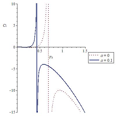
(a) $C_{1}$ for $0\leq r_{h}\leq 1.5$

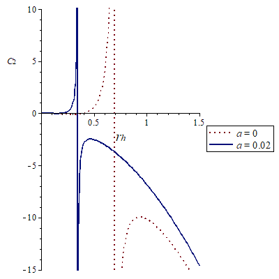
(b) $C_{2}$ for $0\leq r_{h}\leq 1.5$

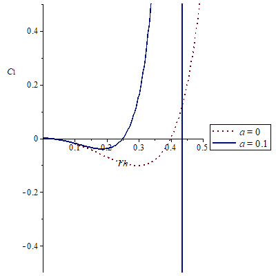
(c) $C_{1}$ for $0\leq r_{h}\leq 0.5$

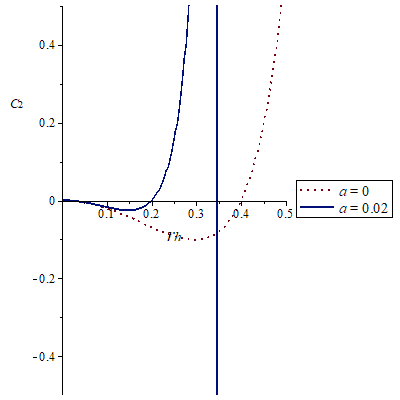
(d) $C_{2}$ for $0\leq r_{h}\leq 0.5$

Figure 2: The heat capacity versus the event horizon radius with $q=0.4$, the dotted curve corresponds to the Reissner-Nordstrom case and the solid curve to the non-minimal case.

On the other hand, the first law of thermodynamics is given by

$$dM=TdS+\phi dq$$ (54)

for a non-rotating black hole with mass $M$ and electromagnetic potential $\phi$. It is interesting to show that the mass $M$ in the first law can be expressed by the Smarr formula Smarr1973

$$M=2TS+\phi Q$$ (55)

for the Reissner-Nordstrom black hole in the Einstein-Maxwell theory.

Furthermore, the Smarr relation can be also obtained from the Komar integral Komar1959 ; Breton2005 ; Balart2017 ; Mazhari2019 with a correction term as

$$M=2TS+q\phi-\frac{1}{2}\int\tau dV$$ (56)

where $\tau$ is the trace of energy-momentum tensor obtaining from the gravitational field equation

$$G_{a}=\kappa^{2}\tau_{a}\$$ (57)

and it can be related with the work density Hayward1998 . In the minimal Einstein-Maxwell case, this relation (56) is automatically satisfied, since the trace of Maxwell energy-momentum tensor is zero. In contrast to the Einstein-Maxwell theory, the non-minimally coupled $Y(R)F^{2}$ theory has a non-vanishing trace of energy-momentum tensor. By taking $\kappa^{2}=8\pi$, the trace is found

$$\tau=\frac{1}{8\pi}*(G_{a}\wedge e^{a})=\frac{R}{8\pi}=-\frac{1}{8\pi}[A^{\prime\prime}+\frac{4A^{\prime}}{r}+\frac{2}{r^{2}}(A-1)]\ .$$ (58)

In order to investigate whether these metric functions (40) and (44) satisfy the Smarr formula we calculate the correction term as

$$\int_{V}\frac{\tau}{2}dV=\frac{1}{16\pi}\int_{r_{h}}^{\infty}R(r)4\pi r^{2}dr=\frac{M}{2}+\frac{r_{h}^{2}A^{\prime}(r_{h})}{4}-\frac{r_{h}}{2}$$ (59)

for the the metric functions. Then we firstly consider the electric potential (41) at the event horizon

$$\phi=\int_{r_{h}}^{\infty}Edr=\frac{q}{r_{h}}-a\frac{e^{-r_{h}}(r_{h}+4)}{4qr_{h}}\ .$$ (60)

Thus the mass obtained from the Smarr formula (56) turns out to be

$$M=\frac{q^{2}+r_{h}^{2}-ae^{-r_{h}}}{2r_{h}}$$ (61)

and it is equal to the mass obtained from $A(r_{h})=0$. The Smarr formula (56) is also satisfied for the second solution (45) similarly, and the mass is found

$$M=\frac{q^{2}+r_{h}^{2}-a(r_{h}^{2}+4r_{h}+6)e^{-r_{h}}}{2r_{h}}\ .$$ (62)

IV Conclusion

In this study, we have considered Noether symmetry approach to find spherically symmetric, static solutions of the non-minimally coupled $Y(R)F^{2}$ theory. By considering the point-like Lagrangian of the $Y(R)F^{2}$ theory with spherical symmetry, we have found a vector field, satisfying the Noether symmetry condition, and the corresponding conserved quantity for any $Y(R)$ function. We have also derived Euler-Lagrange equations from the point-like Lagrangian. Then we have shown that these equations are same with the equations derived from the field equations of the non-minimal model.

We have also given two exact asymptotically flat solutions and the corresponding non-minimal model. Then we have investigated some thermodynamic properties of these solutions such as the Hawking temperature and the heat capacity to determine the thermal stability intervals of the solutions. Furthermore we have shown that the solutions satisfy the the modified Smarr formula for the models with non-zero energy-momentum tensor.

References

• (1) A. de la Cruz-Dombriz, A. Dobado, A.L. Maroto, Black holes in $f(R)$ theories, Phys. Rev. D 80, 124011 (2009), Phys. Rev. D 83(E), 029903, 2011, arXiv:0907.3872 [gr-qc].
• (2) T. Dereli, Γ–. Sert, Non-minimal $R^{\beta}F^{2}$-Coupled Electromagnetic Fields to Gravity and Static, Spherically Symmetric Solutions, Modern Physics Letters A, Volume 26, Issue 20, pp. 1487-1494, 2011, arXiv:1105.4579 [gr-qc].
• (3) T. Dereli, Γ–. Sert, Non-minimal $ln(R)F^{2}$ Couplings of Electromagnetic Fields to Gravity: Static, Spherically Symmetric Solutions, Eur.Phys.J.C71:1589, 2011, arXiv:1102.3863 [gr-qc].
• (4) Γ–. Sert, Gravity and Electromagnetism with Y(R)F2-type Coupling and Magnetic Monopole Solutions, Eur. Phys. J. Plus 127: 152 , 2012, arXiv:1203.0898 [gr-qc].
• (5) Γ–. Sert, Electromagnetic Duality and New Solutions of the Non-minimally Coupled Y(R)-Maxwell Gravity, Mod. Phys. Lett. A, 2013, arXiv:1303.2436 [gr-qc].
• (6) Γ–. Sert, Regular black hole solutions of the non-minimally coupled Y(R) F2 gravity, J. Math. Phys. 57, 032501 (2016), arXiv:1512.01172 [gr-qc]
• (7) M. Adak, Γ–. Akarsu, T. Dereli, Γ–. Sert, Anisotropic inflation with a non-minimally coupled electromagnetic field to gravity, JCAP 11 026 , 2017, arXiv:1611.03393 [gr-qc].
• (8) Γ–zcan Sert, Inflation of the Universe by the Non-minimal $Y(R)F^{2}$ Models, Mod.Phys.Lett. A35 (2019) no.07, 2050037 DOI: 10.1142/S0217732320500376
• (9) Γ–. Sert, M. Adak, Anisotropic cosmological solutions to the $Y(R)F^{2}$ gravity, Modern Physics Letters A, Vol. 33, No. 1 (2019) 1950286, arXiv:1203.1531v7 [gr-qc] .
• (10) F. Mueller-Hoissen, Non-minimal Coupling from Dimensional Reduction of the Gauss-Bonnet action, Physics Letters B, 201, 3, 1988.
• (11) F. Mueller-Hoissen, Modification of Einstein-Yang-Mills theory from dimensional reduction of the Gauss-Bonnet action, Class. Quant. Grav. 5, L35, 1988.
• (12) T. Dereli, G. Üçoluk, Kaluza-Klein reduction of generalised theories of gravity and non-minimal gauge couplings, Class. Q. Grav. 7, 1109, 1990.
• (13) H.A. Buchdahl, On a Lagrangian for non-minimally coupled gravitational and electromagnetic fields, J. Phys. A 12, 1037, 1979.
• (14) A. R. Prasanna, A new invariant for electromagnetic fields in curved space-time, Phys. Lett. 37A, 331, 1971.
• (15) G. W. Horndeski, Conservation of charge and the Einstein–Maxwell field equations, J. Math. Phys. 17, 1980, 1976.
• (16) F. Mueller-Hoissen, and Reinhard Sippel, Spherically symmetric solutions of the non-minimally coupled Einstein-Maxwell equations, Class. Quantum Grav. 5, 1473-1488, 1988.
• (17) I.T. Drummond, S.J. Hathrell, QED vacuum polarization in a background gravitational field and its effect on the velocity of photons, Phys. Rev. D 22, 343, 1980.
• (18) M. S. Turner and L. M. Widrow, Inflation-produced, large-scale magnetic fields, Phys. Rev. D 37, 2743, 1988.
• (19) L. Campanelli, P. Cea, G. L. Fogli and L. Tedesco, Inflation-Produced Magnetic Fields in $R^{n}$ $F^{2}$ and $IF^{2}$ models, Phys.Rev.D77:123002, 2008, arXiv:0802.2630 [astro-ph].
• (20) K. E. Kunze, Large scale magnetic fields from gravitationally coupled electrodynamics, Phys. Rev. D 81, 043526, 2010, [arXiv:0911.1101 [astro-ph.CO]].
• (21) F. D. Mazzitelli and F. M. Spedalieri, Scalar Electrodynamics and Primordial Magnetic Fields, Phys.Rev. D, 52 6694-6699 , 1995, arXiv:astro-ph/9505140.
• (22) K. Bamba and S. D. Odintsov, Inflation and late-time cosmic acceleration in non-minimal Maxwell-F(R) gravity and the generation of large-scale magnetic fields, JCAP 0804:024, 2008, arXiv:0801.0954 [astro-ph].
• (23) S. Capozziello and Lambiase G., Higher-Order Corrections to the Effective Gravitational Action from Noether Symmetry Approach, Gen. Rel. Grav. 32, 295, 2000, arXiv:gr-qc/9912084.
• (24) S. Capozziello, A. Stabile, A. Troisi, Spherically symmetric solutions in $f(R)$-gravity via Noether Symmetry Approach, Class.Quant.Grav.24:2153-2166,2007, arXiv:gr-qc/0703067.
• (25) S. Capozziello and A. De Felice, $f(R)$ cosmology by Noether’s symmetry, JCAP 0808:016, 2008, arXiv:0804.2163 [gr-qc].
• (26) L. Smarr, Mass Formula for Kerr Black Holes, Phys. Rev. Lett. 30, 71, 1973.
• (27) A. Komar, Covariant Conservation Laws in General Relativity, Phys. Rev. 113, 934, 1959.
• (28) N. Breton, Smarr’s formula for black holes with non-linear electrodynamics, Gen.Rel.Grav.37:643-650, 2005, arXiv:gr-qc/0405116.
• (29) L. Balart and S. Fernando, A Smarr formula for charged black holes in nonlinear electrodynamics, Mod. Phys. Lett. A, Vol. 32, No. 39, 1750219, 2017, arXiv:1710.07751 [gr-qc].
• (30) S.H. Mazharimousavi, and M. Halilsoy, Einstein-nonlinear Maxwell–Yukawa black hole, International Journal of Modern Physics D, 28, 09, 1950120, 2019.
• (31) S. A. Hayward, Unified first law of black-hole dynamics and relativistic thermodynamics, Class.Quant.Grav.15:3147-3162, 1998, arXiv:gr-qc/9710089.