Radio linear polarization of GRB afterglows: Instrumental Systematics in ALMA observations of GRB 171205A

Abstract

Polarization measurements of gamma-ray burst (GRB) afterglows are a promising means of probing the structure, geometry, and magnetic composition of relativistic GRB jets. However, a precise treatment of instrumental calibration is vital for a robust physical interpretation of polarization data, requiring tests of and validations against potential instrumental systematics. We illustrate this with ALMA Band 3 (97.5 GHz) observations of GRB 171205A taken $\approx 5.19$ days after the burst, where a detection of linear polarization was recently claimed. We describe a series of tests for evaluating the stability of polarization measurements with ALMA. Using these tests to re-analyze and evaluate the archival ALMA data, we uncover systematics in the polarization calibration at the $\approx 0.09\%$ level. We derive a 3$\sigma$ upper limit on the linearly polarized intensity of $P<97.2~{}\mu$Jy, corresponding to an upper limit on the linear fractional polarization of $\Pi_{\rm L}<0.30\%$, in contrast to the previously claimed detection. Our upper limit improves upon existing constraints on the intrinsic polarization of GRB radio afterglows by a factor of 3. We discuss this measurement in the context of constraints on the jet magnetic field geometry. We present a compilation of polarization observations of GRB radio afterglows, and demonstrate that a significant improvement in sensitivity is desirable for eventually detecting signals polarized at the $\approx 0.1\%$ level from typical radio afterglows.

1. Introduction

Polarization studies of long-duration GRB afterglows are expected to probe the presence of ordered magnetic fields in their jetted outflows as well as the viewing geometry (Granot, 2003; Granot & Königl, 2003; Rossi et al., 2004; Granot & Taylor, 2005; Kobayashi, 2017), yielding crucial constraints on the jet launching mechanism and the central engine (Lyubarsky, 2009; Bromberg & Tchekhovskoy, 2016). Whereas polarization studies in the optical have revealed evidence for structured magnetic fields in the outflow (Steele et al., 2009; Cucchiara et al., 2011; Mundell et al., 2013; Wiersema et al., 2014), similar studies at radio/millimeter (mm) frequencies have been more limited due to instrumental sensitivity constraints (Taylor et al., 1998; Frail et al., 2003; Taylor et al., 2004; Granot & Taylor, 2005; van der Horst et al., 2014; Covino & Gotz, 2016).

The advent of the Atacama Large Millimeter/Sub-millimeter Array (ALMA) is changing the landscape, and has resulted in the first detection of polarized emission from GRBs in the radio/mm band, which has provided preliminary constraints on the magnetic field structure in GRB jets (Laskar et al., 2019). Additionally, Urata et al. (2019) claimed a detection of $(0.27\pm 0.04)\%$ linear polarization in the radio afterglow of GRB 171205A, measured $\approx 5.19$ days after the burst with ALMA at 97.5 GHz. By assuming an intrinsic polarization of $\approx 1\%$, and by ascribing the difference between the intrinsic and observed polarization to depolarization by a population of non-accelerated electrons, they inferred an acceleration fraction of $f_{\rm acc}\approx 0.1$.

As polarization capabilities with ALMA continue to evolve since the initial commissioning effort (Nagai et al., 2016), consistent analysis frameworks need to be deployed to interpret polarization observations, especially in the case of detections near the threshold of the current instrumental systematics. Here, we discuss strategies for testing data for these systematics in polarization measurements of faint sources. We re-analyze the observations reported in Urata et al. (2019), and demonstrate that the data suffer from unremovable, systematic calibration uncertainties.

We report our derived upper limit on the polarization of GRB 171205A in Section 2. We discuss the implications of the upper limit on the magnetic field structure, and compare with previous observations of polarized emission for GRB radio afterglows in Section 3.

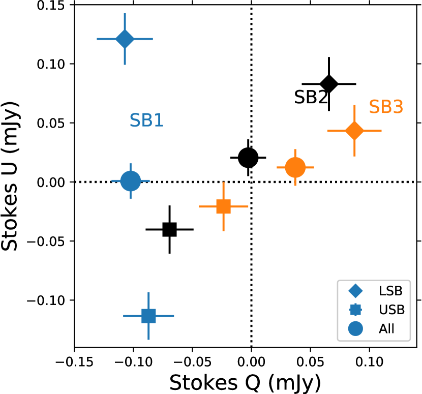
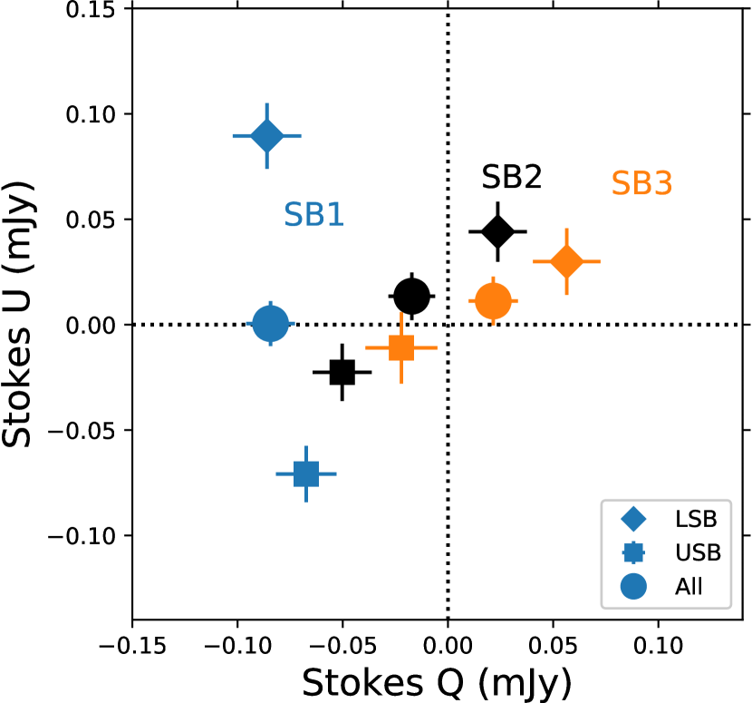
Figure 1.— Stokes $Q$ versus Stokes $U$ before (left) and after (right) self-calibration for GRB 171205A (circles) divided into lower sideband (diamonds) and upper sideband (squares), and further by time into the three executions of the scheduling block at 5.136–5.168 d (blue), 5.174–5.207 d (black), and 5.217–5.245 d (orange). The polarization properties are neither consistent in frequency across ALMA Band 3 (points with the same color), nor stable with time (points with same marker shape). The $QU$ axis scales are equal and are identical between the two panels. Upon self-calibration (see Section 2.2), the uncertainty on the individual measurements is reduced and the points shift closer to the origin (zero polarization). The measurements, which span 2.6 hours, exhibit an unexpectedly strong trend in time, corresponding to a rotation in the plane of polarization from $\approx-44^{\circ}$ to $\approx 31^{\circ}$ for the self-calibrated data.

2. ALMA polarization observations

2.1. QA2 calibration

We downloaded the raw data for full-Stokes ALMA Band 3 (3mm) observations of GRB 171205A taken on 2017 December 10 under project 2017.1.00801.T (PI: Urata) from the ALMA archive. The observations employed J1127-1857 as bandpass and flux density calibrator, J1256-0547 as polarization calibrator, and J1130-1449 as complex gain calibrator. As a first step, we used the CASA (McMullin et al., 2007) calibration scripts, associated with the data set and also available from the ALMA archive, to regenerate the calibrated Quality Assurance 2 (QA2) measurement set. We made images in Stokes $IQUV$ from the full calibrated measurement set with CASA version 5.6.1 using a robust parameter of 0.0, and also independently from the lower sideband (LSB; $89.5$–$93.5$ GHz) and upper sideband (USB; $101.5$–$105.5$ GHz) data. The rms noise near the center of the $Q$, $U$, and $V$ images is ${\approx 7.3}~{}\mu$Jy, consistent with the expected thermal noise given the observation duration. The GRB afterglow is well detected in Stokes $I$, with a flux density of $30.97\pm 0.09$ mJy measured using CASA imfit. The Stokes $I$ image is dynamic range limited, with an rms $\approx 80~{}\mu$Jy. We also detect a point source in maps of Stokes $Q$ and $U$. Fitting for the linearly polarized flux density with the position fixed to that derived from the Stokes $I$ image, we obtain $Q=-68.8\pm 7.3~{}\mu$Jy and $U=-45.6\pm 7.5~{}\mu$Jy, in agreement with the values reported by Urata et al. (2019). However, we find that the Stokes $Q$ measurements differ between the two sidebands by $32~{}\mu$Jy, corresponding to a difference in linear polarization fraction, $\Pi_{\rm L}\approx 0.1\%$ relative to Stokes $I$.

We tested for stability of polarization calibration by dividing the data in time by each execution of the scheduling block (SB), as described in Laskar et al. (2019). This approach reveals systematic trends in the $QU$ time evolution. Stokes $Q$ appears to increase from $-87.8\pm 12.2~{}\mu$Jy to $-48.2\pm 12.2~{}\mu$Jy (a change of $\approx 0.11\%$ of Stokes $I$) over the course of the observations, while Stokes $U$ appears to increase from $-82.4\pm 12.5~{}\mu$Jy to $-20\pm 13.2~{}\mu$Jy ($\approx 0.19\%$ of Stokes $I$), where the uncertainties refer to those associated with the point source fits with imfit, and which are compatible with the expected thermal noise in each SB execution of $\approx 12~{}\mu$Jy. This variability is especially strong in the USB, with $Q$ and $U$ apparently changing by $\approx 0.23\%$ and $\approx 0.30\%$ of Stokes $I$, respectively, over the course of the observations (Fig. 1). The magnitude of these temporal changes are much larger than the absolute value of the polarization detection previously claimed by Urata et al. (2019) with these data.

We also note the presence of significant signal in circular polarization, with Stokes $V=-69.8\pm 7.4~{}\mu$Jy ($\approx 0.23\%$ of $I$), at the same level as the previously claimed linear polarization detection. Circular polarization has only been reported once in a GRB afterglow (Wiersema et al., 2014), and its detection here is more likely indicative of instrumental systematics than of an intrinsic origin. We note that the observed Stokes $V$ is within the current systematic uncertainty for on-axis circular polarization with ALMA ($\approx 0.6$%).

Finally, we also image the gain calibrator (J1130-1449), dividing the data in time into three bins by scheduling block executions. The linear polarization properties of the gain calibrator appear to vary over the course of the observations, with Stokes $Q$ increasing from $8.87\pm 0.04$ mJy (1.11% of Stokes $I$) to $9.79\pm 0.04$ mJy (1.23%; a $\approx 3\sigma$ change, corresponding to 0.12% of $I$) and Stokes $U$ increasing from $-14.85\pm 0.05$ mJy (1.86% of $I$) to $-13.12\pm 0.06$ mJy (1.64%; a $\approx 34\sigma$ change, corresponding to 0.22% of $I$). The gain calibrator also appears to exhibit a statistically significant circular polarization signal, with $V=-1.89\pm 0.05$ mJy (0.24% of $I$). These calibrators are not expected to be significantly circularly polarized in the mm band, and thus the Stokes $V$ measurement most likely indicates residual polarization calibration errors. We discuss this further in Section 2.4.

Table 1Derived polarization properties of the polarization calibrator, J1256-0547

Reference	Method	$Q$	$U$	$\Pi_{\rm L}$	$\chi$
Antenna		(%)	(%)	(%)	(deg)
DV06	qufromgain	$2.08\pm 0.06$	$5.96\pm 0.04$	$6.31$	$35.4$
	XYf+QU	$2.19\pm 0.12$	$5.89\pm 0.03$	$6.29$	$34.8$
	residual	$-0.01\pm 0.09$	$0.07\pm 0.08$	$0.07$	$47.8$
DA64	qufromgain	$2.17\pm 0.15$	$5.99\pm 0.09$	$6.37$	$35.0$
	XYf+QU	$2.20\pm 0.12$	$5.94\pm 0.06$	$6.33$	$34.8$
	residual	$-0.05\pm 0.26$	$0.10\pm 0.23$	$0.11$	$59.3$

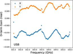
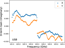
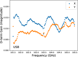
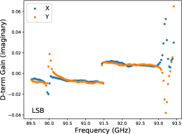
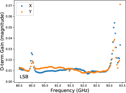
Figure 2.— Real (left column), imaginary (center column), and magnitude (right column) of the derived complex polarization leakage (“$D$-terms”) for antenna DA50 in the upper sideband (USB; upper row) and lower sideband (LSB; lower row) for both $X$ (blue) and $Y$ (orange) polarizations for a reduction using DA64 as reference antenna. The LSB leakage exhibits a peak at $\approx 90$ GHz and a large spike above $\approx 93$ GHz, while the USB leakage has a quasi-periodic structure. These structures are robust to choice of reference antenna used in the polarization calibration (Fig. 3). $D$-term solutions for the other antennas exhibit similar trends.

2.2. Detailed data analysis

Given the apparent instability of polarization properties of the target and phase calibrator with both time and frequency in the QA2 results, we perform a full independent reduction of the data. We import the raw ASDM datasets into CASA, followed by flagging of non-interferometric (e.g. pointing, atmospheric calibration, and sideband ratio) data. We apply the system temperature (Tsys) and water vapor radiometer (wvr) calibrations to the data, and concatenate the three executions of the scheduling block (SB) into a single CASA measurement set.

We perform interferometric and polarization calibration using standard techniques, beginning with deriving the bandpass phase and amplitude calibration, in that order. We use DV06 as reference antenna, and validate our calibration by repeating the entire analysis separately using a nearby antenna with a different architecture, DA64. For the polarization calibration, we first derive the complex gain solutions on the polarization calibrator, and then derive an a priori estimate of its Stokes $Q$ and $U$ from the ratio of complex gains using the python utility qufromgain from the ALMA polarization helpers module (almapolhelpers.py; see CASA documentation for details). The parallactic angle of the polarization calibrator decreases from $\approx 230^{\circ}$ to $\approx 130^{\circ}$ over the course of the observations, providing adequate coverage for disentangling the source and instrumental polarization. The derived fractional $Q$ and $U$ values for the polarization calibrator are consistent across all four spectral windows and across the use of the two different reference antennas, although we note that using DV06 yields a lower estimated uncertainty on $Q$ and $U$ (Table 1). We note that these are fractional polarization values, since they were derived assuming unity Stokes $I$.

To derive the cross-hand delays, we use scan 61 on the polarization calibrator as the scan with the strongest polarization signal, selected based on a plot of the complex polarization ratio for this calibrator as a function of time. We next solve for the $XY$ phase of the reference antenna, the channel-averaged polarization of the polarization calibrator, and the instrumental polarization using the XYf+QU mode in CASA’s gaincal task. The net instrumental polarization averaged across all baselines (as reported by gaincal) varies from $\approx 0.06\%$ to $\approx 0.2\%$ over the four spectral windows. We resolve the $QU$ phase ambiguity with the python utility xyamb using the fractional $Q$ and $U$ derived earlier. We list the final derived values for the fractional polarization of the polarization calibrator in Table 1.

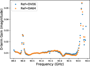
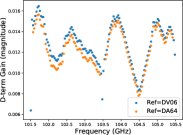
Figure 3.— Magnitude of the polarization leakage for antenna DA50 in the lower sideband (left) and upper sideband (right) derived using independent reductions with two different reference antennas, DV06 (blue) and DA64 (orange). The derived $D$-terms are robust to choice of reference antenna used. $D$-term solutions for the other antennas exhibit similar trends.

We use these derived polarization properties to refine the complex gain solution on the polarization calibrator. We run qufromgain again on the resulting calibration table, which yields a residual polarization statistically indistinguishable from zero, and demonstrates that the source polarization has been successfully removed from the gain solutions. However, we note that the final residual polarization, determined by running qufromgain on the calibrated calibrator data, is $\approx 0.1\%$ (Table 1), suggesting that the minimum systematic uncertainty in polarization measurements from this dataset is at least of this order. Antenna DV22 exhibits large ($\approx 10\%$) residual cross-hand polarization amplitude gain ratios in the 91.5–93.5 GHz spectral window, and we flag that antenna in that spectral window before proceeding.

Finally, we solve for the polarization leakage (antenna “$D$ terms”) using polcal. The derived leakage terms exhibit a strong increase up to $\approx 7\%$ for several antennas at the upper edge ($\gtrsim 93$ GHz) of the LSB, in addition to a weaker peak at $\approx 90$ GHz (Fig. 2). This behavior is seen in both reductions, i.e., independent of the reference antenna used for calibration (Fig. 3). The leakage appears lower and more consistent across channels in the USB, but does exhibit a quasi-periodic structure, as previously also noted in the 3C286 Science Verification data of ALMA Band 6 polarization observations (Nagai et al., 2016).

We set the flux density of J1127-1857 using measurements near the time of the GRB observations listed the ALMA calibrator catalog, from which we derive a spectral index of $\beta=-0.51\pm 0.01$ and a flux density of $\approx 1.05$ Jy at a reference frequency of 91.5 GHz. The derived flux density of the polarization calibrator (J1256-0547) is $12.4871\pm 0.0009$ Jy at the band center reference frequency of 97.287 GHz with a spectral index of $\beta=-0.528\pm 0.001$, and that of the gain calibrator (J1130-1449) is $0.7968\pm 0.0004$ Jy with a spectral index of $\beta=-0.987\pm 0.007$. We complete the calibration by deriving and applying standard interferometric complex antenna gain solutions using the interleaved observations of J1130-1449.

Table 2Impact of self-calibration on ALMA Band 3 (97.5 GHz) Polarization Observations of GRB 171205A

Sideband	Selfcal	Selfcal	$I$	$I_{\rm rms}$	$Q$	$U$	$V$	$P$
	Type	Interval	(mJy)	($\mu$Jy)	($\mu$Jy)	($\mu$Jy)	($\mu$Jy)	($\mu$Jy)
LSB	None	…	$31.68\pm 0.11$	38.0	$-3.2\pm 10.6$	$50.8\pm 11.2$	$-65.2\pm 10.4$	$69.6\pm 15.4$
LSB	phase only	10 min	$32.68\pm 0.03$	15.8	$-4.2\pm 10.7$	$53.9\pm 11.2$	$-67.2\pm 10.3$	$72.9\pm 15.4$
LSB	phase only	2 min	$33.13\pm 0.02$	11.4	$-4.3\pm 10.8$	$55.5\pm 11.4$	$-68.4\pm 10.4$	$73.9\pm 15.5$
LSB	amp & phase	20 min	$33.02\pm 0.03$	11.2	$14.4\pm 10.6$	$72.8\pm 11.4$	$-73.1\pm 10.3$	$86.7\pm 15.6$
LSB	amp & phase	30 s	$33.11\pm 0.03$	10.5	$4.6\pm 10.1$	$72.4\pm 11.6$	$-70.4\pm 10.4$	$87.1\pm 15.2$
USB	None	…	$29.96\pm 0.12$	35.3	$-54.0\pm 10.8$	$-46.3\pm 10.3$	$-69.8\pm 10.4$	$77.5\pm 14.9$
USB	phase only	10 min	$31.18\pm 0.04$	14.7	$-55.5\pm 10.8$	$-44.4\pm 10.5$	$-75.0\pm 10.5$	$75.9\pm 15.0$
USB	phase only	2 min	$31.79\pm 0.03$	12.2	$-57.6\pm 10.8$	$-45.8\pm 10.6$	$-76.9\pm 10.7$	$78.6\pm 15.1$
USB	amp & phase	20 min	$32.00\pm 0.03$	11.3	$-57.2\pm 10.6$	$-44.9\pm 10.4$	$-77.5\pm 10.5$	$77.4\pm 14.9$
USB	amp & phase	30 s	$32.08\pm 0.03$	10.6	$-7.1\pm 10.0$	$-46.1\pm 10.5$	$-77.8\pm 10.5$	$51.5\pm 14.5$
All	None	…	$30.77\pm 0.09$	29.3	$-20.0\pm 7.8$	$13.6\pm 8.1$	$-70.0\pm 7.6$	$37.8\pm 11.2$
All	amp & phase	20 min	$32.44\pm 0.03$	7.7	$-31.5\pm 7.3$	$9.6\pm 7.7$	$-73.4\pm 7.3$	$41.7\pm 10.6$

2.3. Imaging

We combine and image the calibrated measurement set using tclean in CASA with a robust parameter of 0.0 and one Taylor term (i.e. nterms=1). The clean beam is $0\farcs 28$ $\times$ $0\farcs 20$ at a position angle of $85^{\circ}$ The afterglow is well-detected with a flux density of $30.8\pm 0.1$ mJy, measured with a point source model using imfit in CASA. No significant polarization signal is detected at the position of the afterglow in Stokes $Q$, $U$, or in the $P$ image. Our initial estimate for the point source flux density is $\approx 4\%$ lower than the self-calibrated and sideband-combined flux density reported by Urata et al. (2019). However, we caution against a direct flux comparison, since Urata et al. (2019) do not report the flux density or spectral properties of the flux calibrator that they assumed for the analysis.

We note the presence of significant ($\approx 3\%$) cleaning residuals in the Stokes $I$ image, both for the GRB and the phase calibrator, indicating residual calibration errors, potentially due to atmospheric phase decoherence. We correct for these by performing two rounds of phase-only self-calibration with solution intervals of 10 min and 2 min on both the GRB afterglow and phase calibrator data. We split the data into upper and lower sidebands for this step in order to reduce the fractional bandwidth from $\approx 16\%$ for the full dataset to $\approx 4\%$ per sideband, and thus minimize the effect of the frequency structure of the source on the calibration solutions. This is especially important for the calibrator, which exhibits a fitted spectral index (from the gain solutions) of $\approx-0.5$, and thus a potential variation in Stokes $I$ intensity of $\approx 8\%$ across the ALMA band. We solve for a single gain solution for both polarizations (gain mode ‘T’) using gaincal in CASA, in order to avoid introducing a phase offset between the $X$ and $Y$ polarizations. Additionally, we set the reference antenna mode to strict to enforce the use of a single reference antenna during the self-calibration. We continue the use of the same reference antenna for self-calibration as that employed during the earlier calibration steps.

We fit the Stokes $I$ image with a point source model using CASA imfit, followed by fits to the $QUVP$ images with the position and beam parameters fixed to that derived from the Stokes $I$ image. We perform point source fits at each step during the phase-only self-calibration, and present these, together with the Stokes $I$ map rms, in Table 2 for reference. The phase self-calibration reveals low-level ($\approx 2\%$) symmetric residuals indicative of amplitude-based errors. We, therefore, perform one round of amplitude and phase self calibration, applying the pre-derived phase solutions on the fly. Since amplitude self-calibration is a less well constrained problem, we solve for one solution per 20 min, for a total of 14 solutions per polarization per antenna. The derived amplitude solutions exhibit moderate ($\approx 10\%$) variability with time, but the flux density scale remains stable under amplitude self calibration (Table 2).

We find marginally decreasing residuals with shorter solution intervals; however, amplitude self-calibration at intervals shorter than 20 min do not improve the signal-to-noise further. In particular, a 30 s amplitude and phase self-calibration with gains for both polarizations solved independently as performed in Urata et al. (2019) does not yield a measureable improvement in signal-to-noise in Stokes $I$ (Table 2). Furthermore, these symmetric residuals are not completely removable even with 30 s amplitude and phase self-calibration, suggesting that the errors may be baseline-based, rather than antenna-based. Finally, we note that the minimum theoretical solution interval for self-calibration ($t_{\rm solint}$), which is given by

$$\frac{I_{\rm peak}}{\sigma_{I}}>3\sqrt{N-3}\sqrt{\frac{t_{\rm int}}{t_{\rm solint}}},$$ (1)

where is $t_{\rm int}\approx 9.4\times 10^{3}$ s is the total integration time on source, $N=43$ is the number of antennas in the array, $I_{\rm peak}\approx 30$ mJy is the peak intensity of the source used for self-calibration, and $\sigma_{\rm I}\approx 0.1~{}$mJy is the off-source image rms prior to self-calibration, yields $t_{\rm solint}\gtrsim 35$ s. Thus, the 30 s solution interval used by Urata et al. (2019) is shorter than the minimum possible $t_{\rm solint}$ where stable solutions may be expected.

We perform point source fits on our final images (amplitude and phase self-calibrated to 20 min, with the cross-hand phase fixed), as well as on images made using 30 s amplitude and phase self calibration, where the $X$ and $Y$ gains were allowed to vary independently. We find that reducing the solution interval and fitting the cross-hand phase yields only a marginal increase in Stokes $I$ flux density, from $33.02\pm 0.03$ mJy to $33.11\pm 0.03$ mJy in the lower sideband, and from $32.00\pm 0.03$ to $32.08\pm 0.03$ in the upper sideband. For comparison, we also combine the self-calibrated sideband-separated $uv$-data into a single measurement set, and image the entire 4 GHz dataset simultaneously. Except for Stokes $U$ in the LSB, no significant ($\gtrsim 5\sigma$) emission is visible in the Stokes $QUP$ images. On the other hand, significant ($\approx 10\sigma$) circular polarization again appears at the $\approx 0.23\%$ level.

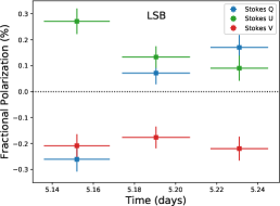
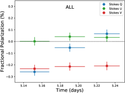
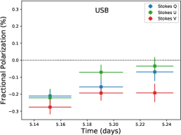
Figure 4.— Fractional Stokes $QUV$ measurements for GRB 171205A (using self-calibrated data) as a function of time relative to the Swift trigger time (center), divided into LSB (left) and USB (right). Each time bin corresponds to one execution of the scheduling block. The fractional uncertainty from the Stokes $I$ measurement is two orders of magnitude smaller than that from the $QUV$ measurements, and is thus ignored. Error bars in the time direction correspond to the span of the data imaged.

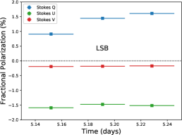
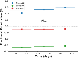
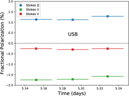
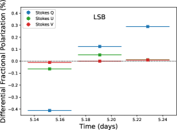
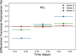
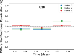
Figure 5.— Upper panels: same as Fig. 4, but for the gain calibrator J1130-1449. The (statistical) uncertainties on each point are typically smaller than the thickness of the line used to plot the horizontal error bar. We find a non-zero Stokes $V$, as well as significant evolution of Stokes $QUV$ with time. The latter effect is clearer with the respective mean values of $QUV$ removed (lower panels; mean subtracted independently for each subplot and polarization). All plots in the same row are on the same scale.

Table 3Stability of ALMA Band 3 Polarization Observations to Time and Frequency Slicing

Target	Sideband	Frequency	SB	$I$	$I_{\rm rms}$	$Q$	$U$	$V$	$P$
		(GHz)	Execution	(mJy)	($\mu$Jy)	($\mu$Jy)	($\mu$Jy)	($\mu$Jy)	($\mu$Jy)
GRB 171205A	LSB	91.463	1	$33.01\pm 0.03$	16.6	$-86.0\pm 15.6$	$89.5\pm 16.3$	$-68.7\pm 14.8$	$140.5\pm 22.4$
GRB 171205A	LSB	91.463	2	$33.04\pm 0.04$	16.1	$23.7\pm 14.3$	$44.0\pm 13.8$	$-58.2\pm 13.8$	$67.0\pm 19.8$
GRB 171205A	LSB	91.463	3	$33.07\pm 0.04$	17.4	$56.4\pm 15.8$	$29.9\pm 16.1$	$-72.5\pm 15.2$	$81.1\pm 22.5$
GRB 171205A	USB	103.495	1	$32.00\pm 0.03$	17.4	$-67.4\pm 13.4$	$-70.9\pm 14.4$	$-88.4\pm 13.5$	$105.3\pm 19.6$
GRB 171205A	USB	103.495	2	$32.01\pm 0.04$	16.9	$-50.3\pm 13.6$	$-22.6\pm 14.0$	$-61.9\pm 14.2$	$61.2\pm 19.6$
GRB 171205A	USB	103.495	3	$32.08\pm 0.04$	18.3	$-22.1\pm 17.0$	$-11.0\pm 17.1$	$-61.7\pm 17.3$	$50.4\pm 24.1$
GRB 171205A	All	97.496	1	$32.46\pm 0.03$	12.5	$-84.3\pm 10.7$	$0.05\pm 11.6$	$-75.6\pm 10.8$	$91.3\pm 15.7$
GRB 171205A	All	97.496	2	$32.52\pm 0.03$	12.2	$-17.2\pm 11.3$	$13.5\pm 11.1$	$-69.7\pm 11.3$	$34.5\pm 15.8$
GRB 171205A	All	97.496	3	$32.54\pm 0.03$	13.8	$21.5\pm 11.6$	$11.2\pm 11.7$	$-68.0\pm 11.9$	$44.1\pm 16.4$
						$Q$ (mJy)	$U$ (mJy)	$V$ (mJy)	$P$ (mJy)
Gain Calibrator	LSB	91.463	1	$847.29\pm 0.08$	69.8	$7.71\pm 0.07$	$-13.50\pm 0.09$	$-1.63\pm 0.05$	$15.5\pm 0.1$
Gain Calibrator	LSB	91.463	2	$847.61\pm 0.08$	69.4	$12.20\pm 0.10$	$-12.52\pm 0.09$	$-1.55\pm 0.05$	$17.5\pm 0.1$
Gain Calibrator	LSB	91.463	3	$847.83\pm 0.08$	68.0	$13.60\pm 0.10$	$-12.86\pm 0.07$	$-1.46\pm 0.05$	$18.8\pm 0.1$
Gain Calibrator	USB	103.495	1	$749.19\pm 0.07$	61.3	$8.52\pm 0.06$	$-13.10\pm 0.08$	$-1.90\pm 0.05$	$15.6\pm 0.1$
Gain Calibrator	USB	103.495	2	$749.17\pm 0.06$	66.2	$8.42\pm 0.09$	$-12.87\pm 0.08$	$-2.23\pm 0.05$	$15.4\pm 0.1$
Gain Calibrator	USB	103.495	3	$749.32\pm 0.06$	62.5	$9.70\pm 0.10$	$-11.8\pm 0.06$	$-1.92\pm 0.06$	$15.3\pm 0.1$
Gain Calibrator	All	97.496	1	$798.9\pm 0.6$	181.6	$8.29\pm 0.07$	$-13.46\pm 0.09$	$-1.95\pm 0.05$	$15.8\pm 0.1$
Gain Calibrator	All	97.496	2	$799.0\pm 0.6$	197.9	$10.50\pm 0.10$	$-12.84\pm 0.09$	$-2.01\pm 0.05$	$16.6\pm 0.1$
Gain Calibrator	All	97.496	3	$799.2\pm 0.6$	177.0	$11.70\pm 0.10$	$-12.49\pm 0.07$	$-1.80\pm 0.05$	$17.1\pm 0.1$

2.4. Polarization measurements

We are unable to reproduce the polarization measurements of Urata et al. (2019) in our analysis. In the lower sideband, our measurements of Stokes $Q$ are statistically indistinguishable from zero, whereas Stokes $U$ appears positive, rather than negative as found by the previous authors. In the upper sideband, the 30 s amplitude self-calibration yields an extremely large change in Stokes $Q$ relative to the 20 min calibration; the Stokes $Q$ flux density changes from $-57.2\pm 10.6~{}\mu$Jy to $-7.1\pm 10.0~{}\mu$Jy, highlighting the danger in leaving the cross-hand phase free while self-calibrating weakly polarized sources. We note that self-calibration moves the $QU$ data points closer to the origin in the $Q$-$U$ plane, corresponding to zero polarization (Fig. 1).

In all cases, our images reveal an unexpected detection in Stokes $V=-69.3\pm 10.0~{}\mu$Jy in the LSB and $V=-77.5\pm 10.5~{}\mu$Jy in the USB, corresponding to a circular polarization at the level of $\approx 0.21\%$–0.24%. This is similar to the level previously noted for the phase calibrator. We caution that the minimum systematic uncertainty in circular polarization measurements with ALMA is currently $\approx 0.6\%$, and hence this (statistically significant) detection of Stokes $V$ is almost certainly spurious and most likely indicates residual (unremovable) calibration errors. These may arise, for instance, from time-variable $XY$ phase or standing waves in the orthomode transducers. Another possibility is that the polarization calibrator has non-zero circular polarization. Standard polarization calibration assumes negligible $V$ in the polarization calibrator. Thus, non-zero $V$ in the calibrator may corrupt the calibration solution, and the calibrator’s $V$ may subsequently appear in calibrated science target data. We note that $I$ to $V$ conversion due to beam squint is expected to be negligible close to the primary beam axis. The level of spurious circular polarization is similar to that of the claimed linear polarization detection in Urata et al. (2019); however, as those authors do not present Stokes $V$ images or photometry, we cannot perform a direct comparison in Stokes $V$. We stress that the systematic calibration errors causing a spurious Stokes $V$ signal may or may not be the same errors causing the spurious $Q$ and $U$ detections we see in the data.

We further test for calibration stability by dividing the data into time bins by each of the three executions of the scheduling block. (Table 3). We find that the polarization measurements exhibit significant time variability. Stokes $Q$ increases by $\approx 0.3\%$ of Stokes $I$, changing sign during the observation from negative to positive (Fig. 4). The change is $\approx 10\sigma$ relative to the typical (statistical) measurement uncertainty in $Q$. The variation is especially pronounced in the LSB ($\approx 0.4\%$ of $I$), and is even larger in the LSB for Stokes $Q$ ($\approx 0.5\%$ of $I$) prior to self-calibration. At the same time, the polarization properties exhibit very different structures in the lower and upper sideband. For instance, Stokes $U$ is positive in the first scheduling block in the LSB ($89\pm 16~{}\mu$Jy), but negative in the USB ($-71\pm 14~{}\mu$Jy). The difference of $\approx 160~{}\mu$Jy between LSB and USB, a factor of $\approx 9$ relative to their mean, cannot arise from the $\approx 3$% difference in their Stokes $I$. Our measurements of Stokes $U$ for the GRB decrease toward zero with time in both sidebands. This trend is robust to self-calibration (Fig. 1). The time scale of this evolution is $\approx 2.6$ hours at $\approx 5.2$ days. The corresponding fractional duration of only $\approx 2\%$ would imply unphysically rapid changes, $\alpha\approx-70$ for an expected power law temporal evolution, $P\propto t^{\alpha}$, ruling out intrinsic changes and implying instabilities in the polarization calibration.

We search for systematic calibration errors by repeating the above analysis for the gain calibrator, J1130-1449. We self-calibrate the data separately in the two sidebands in the same manner as for GRB 171205A. The images reveal statistically significant circular polarization at the level $V\approx 0.25\%$ (sideband-averaged), similar to that obtained in the GRB data. This source has been variously categorized as an optical quasi-stellar object (QSO) and blazar (Massaro et al., 2009; Mignard et al., 2016). QSOs and blazars have been observed to circular polarization at the $\approx 0.1\%$ level at cm wavelengths (Rayner et al., 2000). However, the circular polarization fraction is expected to fall with frequency as $V/I\propto\nu^{\alpha_{\rm V}}$ with $-\alpha_{\rm V}\approx 1$–3 (Pacholczyk, 1973; Melrose, 1997), implying negligible Stokes $V$ at the mm wavelengths employed here. Indeed, very few blazars have detected circular polarization at mm wavelengths (Agudo et al. 2010, 2018; however, see also Thum et al. 2018). Thus, the consistent detected Stokes $V$ for the gain calibrator may imply residual uncorrected instrumental polarization in the data.

We search the gain calibrator data for systematics by investigating variability in the polarization properties in time and frequency. As in the case of the GRB, we find that Stokes $Q$ and $U$ vary by up to $0.4\%$ of Stokes $I$ over time, and the variation is as strong as $\approx 0.7\%$ of Stokes $I$ in the LSB (Fig. 5). Intrinsic variations on the time scale of $\approx 2.6$ hours as observed here are not expected in radio-loud AGN (Dent, 1965). Whereas interstellar scintillation can cause variability on much shorter (hour) time scales, this effect is expected to be negligible at mm wavelengths (Quirrenbach, 1992; Goodman & Narayan, 2006). Thus, the observed strong variability of the polarization properties of the gain calibrator are most likely instrumental and not intrinsic to the source. One possible origin for these systematics may be time-varying $XY$ phase. However, investigating this requires second-order calibration corrections, which are beyond the scope of this work.

2.5. Systematic calibration uncertainty

In light of the observed variability of the GRB and gain calibrator data in time and frequency, we believe the systematic calibration uncertainty for this dataset is larger than the nominal $3\sigma$ value of 0.1% quoted in the ALMA Cycle 4 Technical Handbook, relevant “for the brightest calibrators”. Whereas the Handbook does not clarify this term precisely, calibrators with polarization fraction $\gtrsim 10\%$ are available to ALMA, and thus, with a fractional polarization of $\approx 6.3\%$, J1256-0547 is only moderately strongly polarized.

To quantify the true systematic, we use the observed variability in the polarization of the gain calibrator, and assume that the calibrator’s intrinsic polarization is constant with time over our observations. We observe a maximum deviation of $\Delta\Pi_{\rm L}\approx 0.16$% of Stokes $I$ for the calibrator when both sidebands are combined (this number is $\Delta\Pi_{\rm L}\approx 0.21\%$ prior to self-calibration). If the systematic error is a random (Gaussian) process, then this number would be an overestimate of the intrinsic standard deviation of that random process. The expectation value of the difference between the maximum and minimum (i.e., the range) of three numbers drawn from a unit normal distribution is $3\pi^{-1/2}\approx 1.69$ (Schwarz, 2006). Thus, we estimate an additional $1\sigma$ systematic calibration uncertainty of $\approx 0.16\%/1.69\approx 0.09\%$ for these observations.

In conjunction with the statistical uncertainty of $\approx 0.033\%$ in the linear polarization measurement of the GRB when all the data are combined (Table 1), the total ($1\sigma$) uncertainty in the polarization measurement is $\approx 0.10\%$. This yields a linear polarization measurement of $41.7\pm 32.4~{}\mu$Jy (undebiased), and thus the detection of polarization in this event is only significant at $\approx 1.3\sigma$. Since $P/\sigma_{\rm P}\lesssim\sqrt{2}$, the maximum likelihood estimate for $P$ is $\hat{P}=0$ upon correcting for Rician bias (Vaillancourt, 2006). Even for the total linearly polarized density of $\approx 87~{}\mu$Jy reported in Urata et al. (2019), the addition of a $0.09\%$ systematic uncertainty renders the measurement at best a $\approx 2.7\sigma$ detection. Given the significant variability observed and our inability to reproduce the earlier authors’ results using an independent analysis, we consider these data to provide a $3\sigma$ upper limit of $\lesssim 0.30\%$ (combining systematic and statistical uncertainty, and corresponding to $P\lesssim 97.2~{}\mu$Jy) on the linear polarization of GRB 171205A for the remainder of this work.

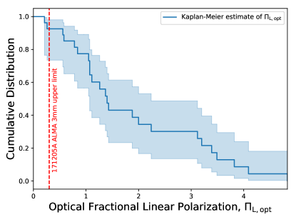
Figure 6.— Kaplan-Meier cumulative distribution function of the optical linear polarization of GRB afterglows observed between 2.6 and 10.4 days (i.e., within a factor of 2 in time relative to the ALMA observations of GRB 171205A), including polarization upper limits, from Covino & Gotz (2016). Between 4–27% of optical afterglow polarization measurements are lower than the ALMA 3mm upper limit of $<0.30\%$ for GRB 171205A (intersection of the dashed line with the shaded region). Thus, we cannot rule out that the linear polarization in this burst is intrinsically low.

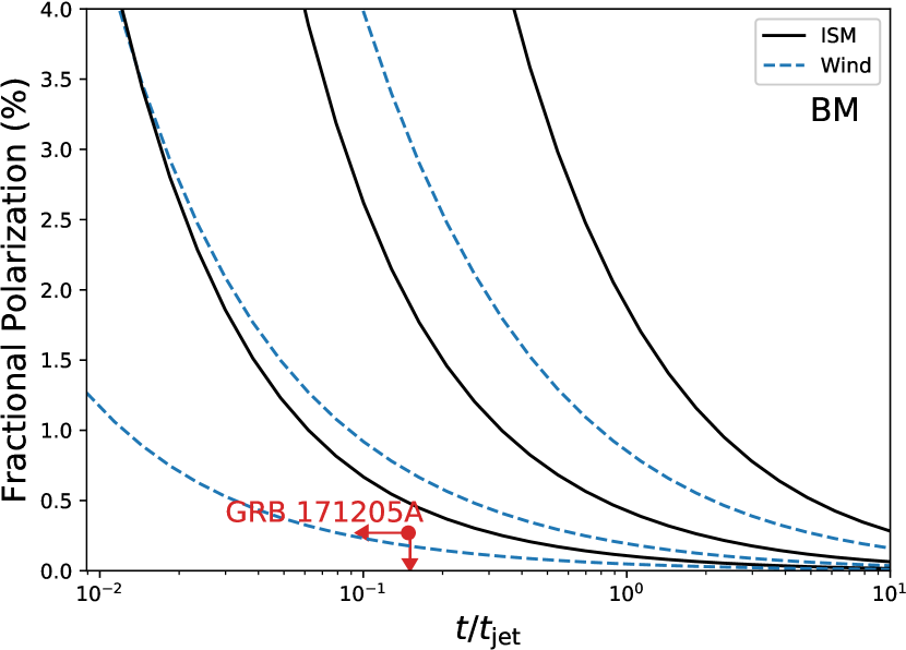
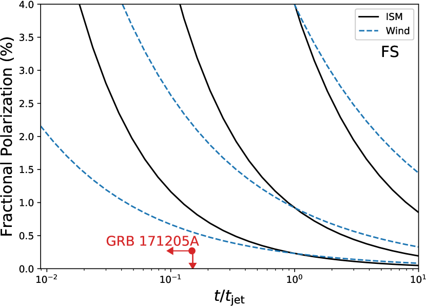
Figure 7.— The expected polarization signature from uniform jets with toroidal magnetic fields expanding into constant density (solid lines) and wind-like environments (dashed lines) for a Blandford-McKee (BM) evolution (left) and FS-like evolution (right), together with the measured polarization fraction upper limit for GRB 171205A (red point). The lower limit on $t_{\rm jet}$ corresponds to $t/t_{\rm jet}\lesssim 0.15$ for the GRB. The three lines are for $\theta_{\rm obs}/\theta_{\rm jet}=0.2$, 0.1, and 0.05, from highest to lowest, respectively. A toroidal magnetic field geometry is difficult to reconcile with the upper limit for most viewing angles if the emission arises from a RS.

3. Discussion

The precise interpretation of the polarization upper limit depends strongly upon whether the emission arises from shocked jet material (i.e., the reverse shock; RS) or from the shocked ambient environment (the forward shock; FS), and upon the magnetic field structure in the region of emission (Ghisellini & Lazzati, 1999; Granot & Königl, 2003; Rossi et al., 2004; Granot & Taylor, 2005). A detailed study of the afterglow emission and its decomposition into forward and reverse shock components is beyond the scope of this work, but we briefly discuss both scenarios. In the case of radiation powered by FS emission and where polarization is the result of viewing a region with shock-produced magnetic fields off-axis, the temporal evolution of the polarization fraction typically exhibits two peaks; however, the polarization fraction can be very low, especially when the viewing geometry is close to being on-axis (Rossi et al., 2004). Thus, we cannot rule this scenario out.

3.1. No strong evidence for thermal electrons

A suppression of the polarization by Faraday depolarization due to a quasi-thermal population of electrons not accelerated at the FS, as argued by Urata et al. (2019), is an interesting possibility (Toma et al., 2008). In their analysis of this burst, Urata et al. (2019) contrast their reported ALMA Band 3 measurement of $\Pi_{\rm L}=(0.27\pm 0.04)\%$ with optical polarization observations (Covino & Gotz, 2016). They claim that optical observations during the FS-dominated phase yield a weighted average optical linear polarization of $\Pi_{\rm L}\approx 1.2$% (without error bars; they also do not describe how they remove any potential RS contamination). They ascribe the difference between the measured and the “typical” optical polarization to the presence of quasi-thermal electrons.

Whereas such a population should indeed exist (Eichler & Waxman, 2005; Sironi & Spitkovsky, 2011), we caution that (i) there is no evidence that radio polarization measurements track the optical polarization (indeed, there is exactly one radio polarization detection of a GRB afterglow to date, with $\Pi_{\rm L,opt}\approx 3\Pi_{\rm L,radio}$; however, the detected optical polarization for that event is likely dominated by extrinsic dust scattering; Laskar et al. 2019; Jordana-Mitjans, N. and Mundell, C. G. and Kobayashi, S. and Smith, R. J. and Guidorzi, C. and Steele, I. A. and Shrestha, M. and Gomboc, A. and Marongiu, M. and Martone, R. and Lipunov, V. and Gorbovskoy, E. S. and Buckley, D. A. H. and Rebolo, R. & Budnev, N. M. ); and (ii) the Urata et al. (2019) analysis ignores the optical polarization upper limits. Including these upper limits, we find that as many as 27% of optical polarization observations made within a factor of 2 in time of the time of these ALMA observations (5.19 days, corresponding to the range $\approx 2.6$–10.4 days) are below the ALMA 3 mm polarization upper limit (Fig. 6). Thus, it is entirely possible that the optical polarization in this burst may have been intrinsically lower than the observed radio upper limit. Futhermore, we note that polarization levels approaching zero can be expected from purely shock-generated fields. Thus, the data do not provide direct observational evidence for non-accelerated particles.

3.2. Constraints on magnetic field geometry

We now discuss the observed upper limit on the polarization at $\approx 5.19$ days in the context of the magnetic field geometry in the jet powering GRB 171205A. In general, the observed polarization degree is a function of the ratio of the off-axis viewing angle ($\theta$) to the opening angle of the jet ($\theta_{\rm jet}$), and the time relative to the jet break time, $t_{\rm jet}$ (Rhoads, 1999; Sari et al., 1999). The X-ray light curve for the afterglow of GRB 171205A exhibits a shallow, unbroken power law decay with $\alpha\approx-1.06$ to $\gtrsim 35$ days, indicating that $t_{\rm jet}\gtrsim 35$ days. Thus, we consider the observation time of $t_{\rm obs}=5.19$ days to correspond to an upper limit on the ratio $t_{\rm obs}/t_{\rm jet}\lesssim 0.15$ days.

Together with coeval Atacama Compact Array (ACA) 345 GHz observations, the ALMA 97.5 GHz data indicate an optically thin spectrum in the mm-band at $\approx 5.19$ days, for which we calculate $\beta_{\rm mm}=-0.51\pm 0.04$. On the other hand, the spectral index between the LSB and USB within Band 3 is lower, $\beta_{\rm 3mm}=-0.25\pm 0.01$, indicating that a spectral break frequency lies not too far below ALMA Band 3. VLA observations at 5–16 GHz around the same time ($\approx 4.3~{}$days) exhibit a steeply rising spectrum, with $\beta_{\rm cm}=1.46\pm 0.03$ (Urata et al., 2019). These observations indicate that both the synchrotron peak frequency ($\nu_{\rm m}$) and self-absorption break ($\nu_{\rm a}$) are at a frequency lower than ALMA Band 3. Furthermore, the VLA spectrum is shallower than the fully self-absorbed expectation of $2\leq\beta_{\rm cm}\leq 2.5$, implying that $\nu_{\rm a}$ is in the cm band at $\approx 5$ days, and that the potential spectral peak near the ALMA band is due to $\nu_{\rm m}$. Therefore depolarization due to synchrotron self-absorption in the ALMA bands is unlikely, indicating that the polarization of the observed radiation is intrinsically low.

We note that RS emission has been seen in ALMA observations of GRB afterglows as late as $\approx 4$ days after the burst (Laskar et al., 2018, 2019). If the radio emission in GRB 171205A arises from adiabatically cooling, reverse-shocked ejecta, then the polarization upper limit presents strong constraints on the magnetic field structure in the GRB jet. For a magnetic field ordered on patches of scale, $\theta_{\rm B}$, the observed polarization would be suppressed by a factor of the number of patches visible, $N\approx(\Gamma\theta_{\rm B})^{-2}$, where $\Gamma$ is the jet Lorentz factor at the time of observations (Nakar & Oren, 2004; Granot & Taylor, 2005). This implies $\theta_{\rm B}\lesssim\Pi_{\rm L,lim}\Gamma^{-1}\Pi_{\rm max}^{-1}\approx 4\times 10^{-3}\Gamma^{-1}$ rad, where we have taken $\Pi_{\rm L,max}=(1-\beta)/(5/3-\beta)\approx 0.68$ (Granot & Taylor, 2005) for $\beta\approx-0.43$ (Urata et al., 2019). This limit is consistent with the value of $\theta_{\rm B}\approx 10^{-3}$ rad inferred from polarization observations of the reverse shock in GRB 190114C (Laskar et al., 2019). Thus, if the emission arises from the reverse shock, this may indicate a universal magnetic field coherence scale.

The low degree of polarization disfavors models of polarization produced by toroidal magnetic fields in GRB jets. To see this, we compare the models of Granot & Taylor (2005) together with the data in Fig. 7. We explore a range of off-axis angles and both constant density and wind-like progenitor environments. For the Lorentz factor evolution of the ejecta after deceleration ($\Gamma\propto R^{-g}$), we consider two scenarios: a minimum value of $g=(3-k)/2$, corresponding to the evolution of the fluid just behind the forward shock, and $g=7/2-k$, a maximum value expected for a reverse shock, corresponding to the Blandford-McKee self-similar solution (Kobayashi, 2000; Granot & Taylor, 2005). In the former case, we find that a toroidal field would produce too high a polarization degree regardless of viewing angle or the circumburst geometry. In the latter case, $\theta_{\rm obs}/\theta_{\rm jet}\approx 0.05$ is marginally allowed by the data; however, this would require a very precise alignment of the jet axis with the line of sight, and is therefore unlikely. Finally, we note that a “universal structured jet” model with a toroidal magnetic field can be ruled out, since it would produce a much higher degree of polarization, $\Pi_{\rm L}\gtrsim 30\%$ at $t\lesssim t_{\rm jet}$ (Lazzati et al., 2004).

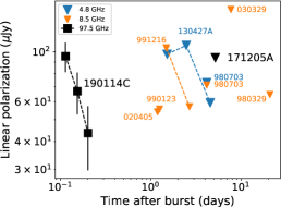
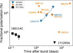
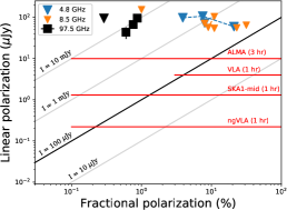
Figure 8.— Linear polarized intensity (left) and fractional linear polarization (center) as a function of observation time for GRB radio afterglows at $\approx 4.8$ GHz (blue), $\approx 8.5$ GHz (orange) and $\approx 97.5$ GHz (black) from this work and collected from the literature (Taylor et al., 1998; Frail et al., 2003; Taylor et al., 2004; Granot & Taylor, 2005; van der Horst et al., 2014; Laskar et al., 2019). The mm-band observations are from ALMA, while the cm-band upper limits are from the VLA, European VLBI Network (130427A), and the Very Long Baseline Array (030329). The bright afterglows of GRB 030329 and 171205A allow for strong upper limits on the fractional polarization, even though the individual upper limits on the polarized intensity are similar to those of other bursts. However, the late observations in these cases most likely precluded a detection. We plot the linear polarized intensity as a function of the polarization fraction in the right panel to compare with the sensitivity of the current and upcoming generations of facilities for a range of Stokes $I$ values from 10 $\mu$Jy to 10 mJy. For typical GRB radio afterglows ($I\approx 100~{}\mu$Jy), polarization observations will be possible with SKA1-mid at the level of $\Pi_{\rm L}\approx 1\%$, but will require full SKA or ngVLA sensitivity for polarization detections at the $\lesssim 0.1\%$ level.

3.3. Radio Polarization of GRB Afterglows

We now compare this derived upper limit to values previously reported for radio observations of GRB afterglows. Our compiled sample of radio linear polarization observations includes one detection (GRB 190114C; Laskar et al., 2019), and several upper limits (GRB 980329, Taylor et al. 1998; GRB 980703, Frail et al. 2003; GRBs 990123, 991216, and 020405, Granot & Taylor 2005; GRB 030329, Taylor et al. 2004; and GRB 130427A, van der Horst et al. 2014; and GRB 171205A, this work).  We convert upper limits listed at different confidence intervals to a uniform $3\sigma$ limit for comparison across events. We multiply the quoted fractional polarization upper limits by the Stokes $I$ flux density to estimate the upper limit in flux density units, and plot these separately at C-band ($\approx 4.8$ GHz), X-band ($\approx 8.5$ GHz), and at 3 mm ($\approx 97.5$ GHz) in Figure 8.

GRB 171205A exhibited the brightest Stokes $I$ flux density of our sample at the time of the polarization observations. Thus, our upper limit on the polarized flux of GRB 171205A, while not the strongest in absolute flux terms, yields the deepest upper limit on the fractional polarization of $\Pi_{\rm L}<0.30\%$ (including systematics). This imposes a factor of 3 stronger constraint on the intrinsic polarization of radio afterglows than previously performed (GRB 030329; Taylor et al., 2004). As discussed in Urata et al. (2019), the emission appears to be optically thin at 97.5 GHz at 5.19 days. Therefore, depolarization due to synchrotron self-absorption is unlikely to be the cause for the non-detection of polarized emission (Toma et al., 2008; Granot & van der Horst, 2014), suggesting that the absence of strongly polarized emission is intrinsic to the source.

We note that the polarization upper limits (and the measurement in the case of GRB 190114C) all lie in the range of $\approx 40$–$150~{}\mu$Jy; the difference in the polarization fractions arises from the large spread (over two orders of magnitude) in Stokes $I$ flux densities in the respective bands at the time of observation. Of these, the ALMA observations of GRB 190114C represent the earliest post-burst polarization-sensitive observations obtained for any mm-band GRB afterglow. The fractional polarization limits in the cm-band are all higher (i.e., worse) than those obtained in the mm-band, indicating the need to improve instrument sensitivity and stability at these frequencies in order to probe polarized emission from GRB afterglows.

According to the ngVLA reference design, the $1\sigma$ point source sensitivity at 8 GHz in 1 hour of on-source integration is $\approx 0.22~{}\mu$Jy. The polarization sensitivity in the current design is expected to be better than $\Pi_{\rm L}\approx 0.1\%$. The required on-source time to detect a typical $\approx 100~{}\mu$Jy GRB afterglow (Chandra & Frail, 2012) polarized at $0.1\%$ will be $\approx 5$ hours, although the source polarization may vary over this same period (Laskar et al., 2019). The full Square Kilometer Array (SKA2) would achieve a similar sensitivity; however, in phase 1, the SKA-mid would require upwards of $56$ hours for a typical GRB radio afterglow.

A detection of linearly polarized radio emission unambiguously associated with the afterglow forward shock would provide the first constraints on the magnetic field structure and viewing geometry for long-duration GRBs (Granot & Königl, 2003). In particular, the evolution of this quantity across the jet break is a sensitive measure of the degree of order in the magnetic fields, the jet structure, and the off-axis viewing angle (Rossi et al., 2004). Thus, we suggest that a more robust interpretation of afterglow polarization requires sensitive measurements (with detections) at multiple epochs. Such observations, while challenging for typical GRBs with ALMA in the mm band, may be routinely tractable with the ngVLA and full SKA.

4. Conclusions

We have presented a series of tests useful for estimating the impact of systematic calibration errors in ALMA polarization data. In particular, we recommend basic sanity checks of (i) dividing the data in time and frequency to test for calibration stability, and (ii) checking the gain calibrator or using test calibrators, if available, to verify and quantify the success of polarization calibration. While these tests have been performed at 3 mm here, they are widely applicable to observations at any frequency.

We have re-analyzed ALMA Band 3 (3 mm) full continuum polarization observations of GRB 171205A taken $\approx 5.19$ days after the burst and performed detailed verification steps to test the stability of polarization calibration. In contrast to previous work (Urata et al., 2019), we do not detect significant linear polarization from the radio afterglow. We find a higher systematic uncertainty than assumed by Urata et al. (2019), and infer a $3\sigma$ upper limit of $P\lesssim 97.2~{}\mu$Jy, corresponding to $\Pi_{\rm L}\lesssim 0.30$% of Stokes $I$, for which we derive a value of $32.44\pm 0.03$ mJy (statistical error). The upper limit on $\Pi_{\rm L}$ is consistent with the range of optical linear polarization observed for GRB afterglows, and thus not immediately indicative of the presence of a population of thermal electrons. If the emission arises in the reverse-shocked region, the upper limit rules out a toroidal magnetic field geometry for most viewing angles, and is consistent with random magnetic field patches of coherence length, $\theta_{\rm B}\lesssim 4\times 10^{-3}$ rad. We have compiled observations of polarized emission in GRB radio afterglows from the literature, and demonstrate that the current observations and limits of linear polarized intensity span a narrow range, likely due to signal-to-noise limitations. We expect that improvements in cm-band polarization sensitivity and stability, such as with the ngVLA and full SKA, will open a new avenue for pursuit of GRB jet structure and magnetization in the future.

References

- Agudo et al. (2010) Agudo, I., Thum, C., Wiesemeyer, H., & Krichbaum, T. P. 2010, ApJS, 189, 1
- Agudo et al. (2018) Agudo, I., Thum, C., Molina, S. N., et al. 2018, MNRAS, 474, 1427
- Bromberg & Tchekhovskoy (2016) Bromberg, O., & Tchekhovskoy, A. 2016, MNRAS, 456, 1739
- Chandra & Frail (2012) Chandra, P., & Frail, D. A. 2012, ApJ, 746, 156
- Condon (1997) Condon, J. J. 1997, PASP, 109, 166
- Covino & Gotz (2016) Covino, S., & Gotz, D. 2016, Astronomical and Astrophysical Transactions, 29, 205
- Cucchiara et al. (2011) Cucchiara, A., Cenko, S. B., Bloom, J. S., et al. 2011, ApJ, 743, 154
- Dent (1965) Dent, W. A. 1965, Science, 148, 1458
- Eichler & Waxman (2005) Eichler, D., & Waxman, E. 2005, ApJ, 627, 861
- Frail et al. (2003) Frail, D. A., Yost, S. A., Berger, E., et al. 2003, ApJ, 590, 992
- Ghisellini & Lazzati (1999) Ghisellini, G., & Lazzati, D. 1999, MNRAS, 309, L7
- Goodman & Narayan (2006) Goodman, J., & Narayan, R. 2006, ApJ, 636, 510
- Granot (2003) Granot, J. 2003, ApJ, 596, L17
- Granot & Königl (2003) Granot, J., & Königl, A. 2003, ApJ, 594, L83
- Granot & Taylor (2005) Granot, J., & Taylor, G. B. 2005, ApJ, 625, 263
- Granot & van der Horst (2014) Granot, J., & van der Horst, A. J. 2014, Publications of the Astronomical Society of Australia, 31, e008
- (17) Jordana-Mitjans, N., Mundell, C. G., Kobayashi, S., et al. 2020, ApJ, 892, 97
- Kobayashi (2000) Kobayashi, S. 2000, ApJ, 545, 807
- Kobayashi (2017) Kobayashi, S. 2017, Galaxies, 5, 80
- Laskar et al. (2018) Laskar, T., Alexander, K. D., Berger, E., et al. 2018, ApJ, 862, 94
- Laskar et al. (2019) Laskar, T., van Eerten, H., Schady, P., et al. 2019, ApJ, 884, 121
- Laskar et al. (2019) Laskar, T., Alexander, K. D., Gill, R., et al. 2019, ApJL, 878, L26
- Lazzati et al. (2004) Lazzati, D., Covino, S., Gorosabel, J., et al. 2004, A&A, 422, 121
- Lyubarsky (2009) Lyubarsky, Y. 2009, ApJ, 698, 1570
- Massaro et al. (2009) Massaro, E., Giommi, P., Leto, C., et al. 2009, A&A, 495, 691
- McMullin et al. (2007) McMullin, J. P., Waters, B., Schiebel, D., Young, W., & Golap, K. 2007, in Astronomical Society of the Pacific Conference Series, Vol. 376, Astronomical Data Analysis Software and Systems XVI, ed. R. A. Shaw, F. Hill, & D. J. Bell, 127
- Melrose (1997) Melrose, D. B. 1997, Journal of Plasma Physics, 58, 735
- Mignard et al. (2016) Mignard, F., Klioner, S., Lindegren, L., et al. 2016, A&A, 595, A5
- Mundell et al. (2013) Mundell, C. G., Kopaˇc, D., Arnold, D. M., et al. 2013, Nature, 504, 119
- Nagai et al. (2016) Nagai, H., Nakanishi, K., Paladino, R., et al. 2016, ApJ, 824, 132
- Nakar & Oren (2004) Nakar, E., & Oren, Y. 2004, ApJ, 602, L97
- Pacholczyk (1973) Pacholczyk, A. G. 1973, MNRAS, 163, 29P
- Quirrenbach (1992) Quirrenbach, A. 1992, Reviews in Modern Astronomy, 5, 214
- Rayner et al. (2000) Rayner, D. P., Norris, R. P., & Sault, R. J. 2000, MNRAS, 319, 484
- Rhoads (1999) Rhoads, J. E. 1999, ApJ, 525, 737
- Rossi et al. (2004) Rossi, E. M., Lazzati, D., Salmonson, J. D., & Ghisellini, G. 2004, MNRAS, 354, 86
- Sari et al. (1999) Sari, R., Piran, T., & Halpern, J. P. 1999, ApJ, 519, L17
- Schwarz (2006) Schwarz, C. R. 2006, Journal of Surveying Engineering, 132, 155
- Sironi & Spitkovsky (2011) Sironi, L., & Spitkovsky, A. 2011, ApJ, 726, 75
- Steele et al. (2009) Steele, I. A., Mundell, C. G., Smith, R. J., Kobayashi, S., & Guidorzi, C. 2009, Nature, 462, 767
- Taylor et al. (2004) Taylor, G. B., Frail, D. A., Berger, E., & Kulkarni, S. R. 2004, ApJ, 609, L1
- Taylor et al. (1998) Taylor, G. B., Frail, D. A., Kulkarni, S. R., et al. 1998, ApJ, 502, L115
- Thum et al. (2018) Thum, C., Agudo, I., Molina, S. N., et al. 2018, MNRAS, 473, 2506
- Toma et al. (2008) Toma, K., Ioka, K., & Nakamura, T. 2008, ApJ, 673, L123
- Urata et al. (2019) Urata, Y., Toma, K., Huang, K., et al. 2019, ApJ, 884, L58
- Vaillancourt (2006) Vaillancourt, J. E. 2006, PASP, 118, 1340
- van der Horst et al. (2014) van der Horst, A. J., Paragi, Z., de Bruyn, A. G., et al. 2014, MNRAS, 444, 3151
- Wiersema et al. (2014) Wiersema, K., Covino, S., Toma, K., et al. 2014, Nature, 509, 201