Dynamics from symmetries in chiral $SU(N)$ gauge theories

Abstract

The symmetries and dynamics of simple chiral $SU(N)$ gauge theories, with matter Weyl fermions in a two-index symmetric tensor and $N+4$ anti-fundamental representations, are examined, by taking advantage of the recent developments involving the ideas of generalized symmetries, gauging of discrete center 1-form symmetries and mixed ’t Hooft anomalies. This class of models are particularly interesting because the conventional ’t Hooft anomaly matching constraints allow a chirally symmetric confining vacuum, with no condensates breaking the $U(1)\times SU(N+4)$ flavor symmetry, and with certain set of massless baryonlike composite fermions saturating all the associated anomaly triangles. Our calculations show that in such a vacuum the UV-IR matching of some $0$-form$-$$1$-form mixed ’t Hooft anomalies fails. This implies, for the theories with even $N$ at least, that a chirally symmetric confining vacuum contemplated earlier in the literature actually cannot be realized dynamically. In contrast, a Higgs phase characterized by some gauge-noninvariant bifermion condensates passes our improved scrutiny.

1 Introduction

In spite of the bulk of knowledge accumulated after almost half-century of studies of vectorlike gauge theories such as $SU(3)$ quantum chromodynamics (QCD), partially based on ever more sophisticated but basically straightforward approximate calculations (lattice simulations), as well as some beautiful theoretical developments in models with ${\cal N}=1$ or ${\cal N}=2$ supersymmetries AffleckDineSei -Cachazo , SW ; Tachikawa , surprisingly little is known today about strongly-coupled ordinary (nonsupersymmetric) chiral gauge theories. Perhaps it is not senseless to make some more efforts to try to understand this class of theories, which Nature might be making use of, in a way as yet unknown to us.

Such a consideration has led two of us recently to give a systematic look into possible phases of a large class of chiral gauge theories BKS ; BK , the first with M. Shifman. To be concrete, we limited ourselves to $SU(N)$ gauge theories with a set of Weyl fermions in a reducible complex representation of $SU(N)$. The gauge interactions in these models become strongly coupled in the infrared. There are no gauge-invariant bifermion condensates, no mass terms or potentials (of renormalizable type) can be added to deform the theories, including the $\theta$ term, and the vacuum is unique.

The questions we addressed ourselves to are: (i) Do these systems confine, or experience a dynamical Higgs phenomenon (dynamical gauge symmetry breaking)?   (ii) Do some of them flow into an IR fixed-point CFT?   (iii) Does the chiral flavor symmetry remain unbroken, or if spontaneously broken, in which pattern?   (iv) If there are more than one apparently possible dynamical scenarios, which one is actually realized in the infrared?   (v) Does the system generate hierarchically disparate mass scales, such as the ones proposed in the "tumbling" scenarios Raby ? and so on. The general conclusion is that the consideration based on the ’t Hooft anomaly matching conditions th and on some other consistency conditions do restrict the list of possible dynamical scenarios, but are not sufficiently stringent BKS -Goity . A more powerful theoretical reasoning is clearly wanted.

Recently the concept of generalized symmetries AhaSeiTac ; GKSW has been applied to Yang-Mills theories and QCD like theories, to yield new, stronger, version (involving $0$-form and $1$-form symmetries together) of ’t Hooft anomaly matching constraints GKKS -BKL . The generalized symmetries do not act on local field operators, as in conventional symmetry operations, but only on extended objects, such as closed line or surface operators. The generalized symmetries are all Abelian AhaSeiTac ; GKSW . This last fact was crucial in the recent extension of these new techniques with color $SU(N)$ center ${\mathbb{Z}}_{N}$ to theories with fermions in the fundamental representation. The presence of such fermions in the system would normally simply break the center ${\mathbb{Z}}_{N}$ symmetry and would prevent us from applying these new techniques. A color-flavor locking by using appropriate discrete subgroups of global $U(1)$ symmetries associated with fermion fields, actually allows us to extend the use of $SU(N)$ center ${\mathbb{Z}}_{N}$ symmetries in those theories.

A key ingredient of these developments is the idea of "gauging a discrete symmetry", i.e., identifying the field configurations related by the $1$-form (or a higher-form) symmetries, and eliminating the consequent redundancies, effectively modifying the path-integral summation rule over gauge fields KapSei ; Seiberg . Since these generalized symmetries are symmetries of the models considered, even though they act differently from the conventional ones, it is up to us to decide to "gauge" these symmetries. Anomalies we encounter in doing so, are indeed obstructions of gauging a symmetry, i.e., a ’t Hooft anomaly by definition. And as in the usual application of the ’t Hooft anomalies such as the "anomaly matching" between UV and IR theories, a similar constraint arises in considering the generalized symmetries together with a conventional ("0-form") symmetry, which has come to be called in recent literature as a "mixed ’t Hooft anomaly". Another term of "global inconsistency" was also used to describe a related phenomenon.

In this paper we take a few, simplest chiral gauge theories as exercise grounds, and ask whether these new theoretical tools can be usefully applied to them, and whether they provide us with new insights into the infrared dynamics and global symmetry realizations of these models.

For clarity of presentation, we focus the whole discussion here on a single class of models (${\psi\eta}$ models BKS ; BK ). In Sec. 2 we review the symmetry and earlier results on the possible phases of these theories. In Sec. 3 the symmetry group of the systems is discussed more carefully, by taking into account its global aspects. Sec. 4 and Sec. 5 contain the derivation of the anomalies in odd $N$ and even $N$ theories, respectively. In Sec. 6 we discuss the UV-IR matching constraints of certain $0$-form and $1$-form mixed anomalies, and their consequences on the IR dynamics in even $N$ theories. In Sec. 7 the mixed anomalies are reproduced without using the Stora-Zumino descent procedure adopted in Sec. 6. Summary of our analysis and Discussion are in Sec. 8. We shall come back to more general classes of chiral theories in a separate work.

2 The model and the possible phases

The model we consider in this work is an $SU(N)$ gauge theory with Weyl fermions

$$\psi^{\{ij\}}\,,\quad\eta_{i}^{B}\,,\qquad({\footnotesize i,j=1,2,\ldots,N\;,\quad B=1,2,\ldots,N+4})\;,$$ (1)

in the direct-sum representation

$$\yng(2)\oplus(N+4)\,{\bar{{\yng(1)}}}\;$$ (2)

of $SU(N)$. This model was studied in ACSS ; ADS , BKS ; BK . This is the simplest of the class of chiral gauge theories known as Bars-Yankielowicz models BY . The first coefficient of the beta function is

$$b_{0}=11N-(N+2)-(N+4)=9N-6\;.$$ (3)

The fermion kinetic term is given by

$$\overline{\psi}\gamma^{\mu}\big{(}\partial+\mathcal{R}_{\mathrm{S}}(a)\big{)}_{\mu}P_{\mathrm{L}}\psi+\sum_{B=1}^{N+4}\overline{\eta_{B}}\gamma^{\mu}\big{(}\partial+\mathcal{R}_{\mathrm{F}^{*}}(a)\big{)}_{\mu}P_{\mathrm{L}}\eta_{B}\;,$$ (4)

with an obvious notation. In order to emphasize that this is the chiral gauge theory, we explicitly write the chiral projector $P_{\mathrm{L}}=\frac{1-\gamma_{5}}{2}$ in the fermion kinetic terms. The symmetry group is

$$SU(N)_{\mathrm{c}}\times SU(N+4)\times U(1)_{\psi\eta}\;,$$ (5)

where $U(1)_{\psi\eta}$ is the anomaly-free combination of $U(1)_{\psi}$ and $U(1)_{\eta}$,

$$U(1)_{\psi\eta}:\ \psi\to\mathrm{e}^{\mathrm{i}(N+4)\alpha}\psi\;,\qquad\eta\to\mathrm{e}^{-\mathrm{i}(N+2)\alpha}\eta\;.\qquad\alpha\in\mathbbm{R}\;.$$ (6)

The group (5) is actually not the true symmetry group of our system, but its covering group. It captures correctly the local aspects, e.g., how the group behaves around the identity element, and thus is sufficient for the consideration of the conventional, perturbative triangle anomalies associated with it, reviewed below in this section.

Its global structures however contain some redundancies, which must be modded out appropriately in order to eliminate the double counting. They furthermore depend crucially on whether $N$ is odd or even. These questions will be studied more carefully in Sec. 3, as they turn out to be central to the main theme of this work: the determination of the mixed anomalies and the associated, generalized ’t Hooft anomaly matching conditions.

2.1 Chirally symmetric phase

It was noted earlier ACSS ; ADS ; BKS that the standard ’t Hooft anomaly matching conditions associated with the continuous symmetry group $U(1)_{\psi\eta}\times SU(N+4)$ allowed a chirally symmetric, confining vacuum in the model. Let us indeed assume that no condensates form, the system confines, and the flavor symmetry is unbroken. The candidate massless composite fermions ("baryons") are:

$${\cal B}^{[AB]}=\psi^{ij}\eta_{i}^{A}\eta_{j}^{B}\;,\qquad A,B=1,2,\ldots,N+4\;,$$ (7)

antisymmetric in $A\leftrightarrow B$. All the $SU(N+4)\times U(1)_{\psi\eta}$ anomaly triangles are saturated by ${\cal B}^{[AB]}$ as can be seen by inspection of Table 1.

	fields	$SU(N)_{\rm c}$	$SU(N+4)$	${U}(1)_{\psi\eta}$
i UV	$\psi$	${\yng(2)}$	$\frac{N(N+1)}{2}\cdot(\cdot)$	$N+4$
	$\eta^{A}$	$(N+4)\cdot{\bar{\yng(1)}}$	$N\,\cdot\,{\yng(1)}$	$-(N+2)$
IR	${\cal B}^{[AB]}$	$\frac{(N+4)(N+3)}{2}\cdot(\cdot)$	${\yng(1,1)}$	$-N$

Table 1: Chirally symmetric phase of the $(1,0)$ model. The multiplicity, charges and the representation are shown for each set of fermions. $(\cdot)$ stands for a singlet representation.

2.2 Color-flavor locked Higgs phase

As the theory is very strongly coupled in the infrared (see (3)), it is also natural to consider the possibility that a bifermion condensate

$$\langle\psi^{\{ij\}}\eta_{i}^{B}\rangle=\,c\,\Lambda^{3}\delta^{jB}\neq 0\;,\qquad j,B=1,2,\dots N\;,\qquad c\sim O(1)$$ (8)

forms. $\Lambda$ is the renormailization-invariant scale dynamically generated by the gauge interactions. The color gauge symmetry is completely (dynamically) broken, leaving however color-flavor diagonal $SU(N)_{\rm cf}$ symmetry

$$SU(N)_{\rm cf}\times SU(4)_{\rm f}\times U(1)^{\prime}\,,$$ (9)

where $U(1)^{\prime}$ is a combination of $U(1)_{\psi\eta}$ and the elements of $SU(N+4)$ generated by

$$\left(\begin{array}[]{cc}-2\,\mathbf{1}_{N}&\\ &\frac{N}{2}\mathbf{1}_{4}\end{array}\right)\;.$$ (10)

As (9) is a subgroup of the original full symmetry group (5) it can be quite easily verified, by making the decomposition of the fields in the direct sum of representations in the subgroup, that a subset of the same baryons ${\cal B}^{[AB]}$ saturate all of the triangles associated with the reduced symmetry group. See Table 2.

	fields	$SU(N)_{\rm cf}$	$SU(4)_{\rm f}$	$U(1)^{\prime}$	$({\mathbb{Z}}_{2})_{F}$
i UV	$\psi$	${\yng(2)}$	$\frac{N(N+1)}{2}\cdot(\cdot)$	$N+4$	$1$
	$\eta^{A_{1}}$	${\bar{\yng(2)}}\oplus{\bar{\yng(1,1)}}$	$N^{2}\,\cdot\,(\cdot)$	$-(N+4)$	$-1$
	$\eta^{A_{2}}$	$4\cdot{\bar{\yng(1)}}$	$N\,\cdot\,{\yng(1)}$	$-\frac{N+4}{2}$	$-1$
IR	${\cal B}^{[A_{1}B_{1}]}$	${\bar{\yng(1,1)}}$	$\frac{N(N-1)}{2}\cdot(\cdot)$	$-(N+4)$	$-1$
	${\cal B}^{[A_{1}B_{2}]}$	$4\cdot{\bar{\yng(1)}}$	$N\,\cdot\,{\yng(1)}$	$-\frac{N+4}{2}$	$-1$

Table 2: Color-flavor locked phase in the $\psi\eta$ model, discussed in Sec. 2.2. $A_{1}$ or $B_{1}$ stand for $1,2,\ldots,N$, $A_{2}$ or $B_{2}$ the rest of the flavor indices, $N+1,\ldots,N+4$. The fermion parity $\psi\to-\psi$, $\eta\to-\eta$ is defined below, Eq. (29).

ciao

The low-energy degrees of freedom are $\tfrac{(N+4)(N+3)}{2}$ massless baryons in the first, symmetric phase of Sec. 2.1, and $\tfrac{N^{2}+7N}{2}$ massless baryons together with $8N+1$ Nambu-Goldstone (NG) bosons, in the second. They represent physically distinct phases. The general consensus so far has been that it was not known which of the phases, Sec. 2.1, Sec. 2.2, or some other phase, was realized in this model. We shall see below that our analysis based on the mixed anomalies and generalized ’t Hooft anomaly matching constraints strongly favors the dynamical Higgs phase, with bifermion condensate (8). The chirally symmetric phase of Sec. 2.1 will be found to be inconsistent.

3 Symmetry of the system

In this section we examine the symmetry of the system more carefully, taking into account the global aspects of the color and flavor symmetry groups. This is indispensable for the study of the generalized, mixed ’t Hooft anomalies, as will be seen below.

The classical symmetry group of our system is given by

$$G_{\mathrm{class}} = G_{\mathrm{c}}\times G_{\mathrm{f}}$$ (11)

$$= SU(N)_{\mathrm{c}}\times\frac{U(1)_{\psi}\times U(N+4)_{\eta}}{\mathbb{Z}_{N}}\;.$$

The color group is $G_{\mathrm{c}}=SU(N)_{c}$, and its center acts non-trivially on the matter fields:

$$\mathbb{Z}_{N}:\psi\to\mathrm{e}^{\frac{4\pi\mathrm{i}n}{N}}\psi\;,\qquad\eta\to\mathrm{e}^{-\frac{2\pi\mathrm{i}n}{N}}\eta\;,\qquad n\in\{1,\dots,N\}\;.$$ (12)

The flavor group is $G_{\mathrm{f}}=\frac{U(1)_{\psi}\times U(N+4)_{\eta}}{\mathbb{Z}_{N}}$. The division by $\mathbb{Z}_{N}$ is understood by the fact that the numerator overlaps with the center of the gauge group, so this has to be factored out in order to avoid double counting. Another, equivalent way of writing the flavor part of the classical symmetry group is

$$G_{\mathrm{f}}=\frac{U(1)_{\psi}\times U(1)_{\eta}\times SU(N+4)}{\mathbb{Z}_{N}\times\mathbb{Z}_{N+4}}\;.$$ (13)

Quantum mechanically one must consider the effects of the anomalies which reduce the flavor group down to its anomaly-free subgroup. This reduction of the symmetry is compactly summarized by the ’t Hooft instanton effective vertex

$${\cal L}_{\rm eff}\sim\mathrm{e}^{-S_{\mathrm{inst}}}\psi^{N+2}\prod_{B=1}^{N+4}\eta^{B}\;,$$ (14)

(where the color, spin and spacetime indices are suppressed) as is well known. This vertex explicitly breaks the independent $U(1)$ rotations for $\psi$ and $\eta$. Three different sub-groups left unbroken can be easily seen from (14). First there is the discrete sub-group of $U(1)_{\psi}$:

$$(\mathbbm{Z}_{N+2})_{\psi}:\ \psi\to\mathrm{e}^{\frac{2\pi\mathrm{i}k}{N+2}}\psi\;,\;\qquad k\in\{1,\dots,N+2\}\;,$$ (15)

which leaves $\eta$ invariant. Then there is the discrete sub-group of $U(1)_{\eta}$:

$$(\mathbbm{Z}_{N+4})_{\eta}:\ \eta\to\mathrm{e}^{\frac{2\pi\mathrm{i}p}{N+4}}\eta\;,\;\qquad p\in\{1,\dots,N+4\}$$ (16)

which leaves $\psi$ invariant. Finally there is a continuous anomaly-free combination of $U(1)_{\psi}$ and $U(1)_{\eta}$:

$$U(1)_{\psi\eta}:\ \psi\to\mathrm{e}^{\mathrm{i}(N+4)\alpha}\psi\;,\qquad\eta\to\mathrm{e}^{-\mathrm{i}(N+2)\alpha}\eta\;.\qquad\alpha\in\mathbbm{R}\;.$$ (17)

The question that arises now is which is the correct anomaly-free sub-group of $U(1)_{\psi}\times U(1)_{\eta}$. Clearly all the three listed above are part of the anomaly-free sub-group, but one must find the minimal description, in order to avoid the double-counting. It is actually sufficient to consider only $U(1)_{\psi\eta}$ with one of the two discrete group. For example by combining the generator of $(\mathbbm{Z}_{N+2})_{\psi}$ with $k=1$ with the element of $U(1)_{\psi\eta}$ with $\alpha=-\frac{2\pi}{(N+2)(N+4)}$ one can obtain the generator of $(\mathbbm{Z}_{N+4})_{\eta}$. But still $U(1)_{\psi\eta}\times(\mathbbm{Z}_{N+2})_{\psi}$ contains redundancies.

From this point on, we must distinguish the two cases, $N$ odd or $N$ even.

3.1 Odd $N$ theories

For odd $N$, the $U(1)_{\psi\eta}$ transformation parameter $\alpha$, Eq. (17), exhibits $2\pi$ periodicity. If we consider the torus $U(1)_{\psi}\times U(1)_{\eta}$, $U(1)_{\psi\eta}$ is a circle that winds $N+4$ times in the $\psi$ direction and $-(N+2)$ times in the $\eta$ direction before coming back to the origin. See Fig. 1 for the case $N=3$ where the torus is described as a square with the edges identified, the four corners all correspond to the identity of the group.

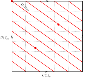
Figure 1: The torus $U(1)_{\psi}\times U(1)_{\eta}$ for $N=3$. The edges are identified as the arrows show, the corners represent the identity of the group. The unbroken subgroup $U(1)_{\psi\eta}$ (red line) passing through all the points of the lattice $(\mathbbm{Z}_{5})_{\psi}\times(\mathbbm{Z}_{7})_{\eta}$. The dots indicate the elements of the center of the gauge group $\mathbbm{Z}_{3}$.

Both $(\mathbbm{Z}_{N+2})_{\psi}$ and $(\mathbbm{Z}_{N+4})_{\eta}$ are sub-groups of the anomaly-free $U(1)_{\psi\eta}$. For example by taking $\alpha=\frac{2\pi}{N+2}\frac{(N+2)+1}{2}$ in (17) $\eta$ is left invariant and we recover exactly the generator of $(\mathbbm{Z}_{N+2})_{\psi}$. The anomaly-free flavor group for odd $N$ is thus:

$$G_{\mathrm{f}}=\frac{U(1)_{\psi\eta}\times SU(N+4)}{\mathbb{Z}_{N}\times\mathbb{Z}_{N+4}}\;.$$ (18)

The division by $\mathbb{Z}_{N}$ is due to the fact that the numerator, $U(1)_{\psi\eta}\times SU(N+4)$, overlaps with the center of the gauge group $\mathbb{Z}_{N}\subset SU(N)$. To see this, we ask whether a $U(1)_{\psi\eta}$ transformation Eq. (17) can act as the minimal element of ${\mathbb{Z}}_{N}\subset SU(N)$:

$$\psi\to\mathrm{e}^{-\frac{4\pi\mathrm{i}}{N}}\psi\;,\qquad\eta\to\mathrm{e}^{\frac{2\pi\mathrm{i}}{N}}\eta\;.$$ (19)

The solution is

$$\alpha={2\pi\over N}\frac{N-1}{2}\;,$$ (20)

as can be easily verified.

The division by $\mathbb{Z}_{N+4}$ can be understood in a similar manner: we consider $U(1)_{\psi\eta}$ with

$$\alpha={2\pi\over N+4}\frac{N+3}{2}\;,$$ (21)

this element acts on fields as

$$\psi\to\psi\;,\qquad\eta\to\mathrm{e}^{-\frac{2\pi\mathrm{i}}{N+4}}\eta\;,$$ (22)

which is the center of $SU(N+4)$ flavor symmetry.

The charges of the fields for odd $N$ theory are the same as given in Table 1.

3.1.1 A remark

The choice of the generator of ${\mathbbm{Z}}_{N}$, (19) is a little arbitrary. If one required instead

$$\psi\to\mathrm{e}^{\frac{4\pi\mathrm{i}}{N}}\psi\;,\qquad\eta\to\mathrm{e}^{-\frac{2\pi\mathrm{i}}{N}}\eta\;,$$ (23)

to be reproduced by $U(1)_{\psi\eta}$ the solution would be

$$\alpha={2\pi\over N}\frac{N+1}{2}\;.$$ (24)

Similarly for ${\mathbbm{Z}}_{N+4}$,

$$\psi\to\psi\;,\qquad\eta\to\mathrm{e}^{\frac{2\pi i}{N+4}}\,\eta\;,$$ (25)

can be reproduced by a $U(1)_{\psi\eta}$ rotation with

$$\alpha={2\pi\over N+4}\frac{N+5}{2}\;.$$ (26)

The charges appearing in (44) below would have to be modified accordingly as

$$\frac{N-1}{2}\to\frac{N+1}{2}\;;\qquad\frac{N+3}{2}\to\frac{N+5}{2}\;.$$ (27)

The conclusion of Sec. 4 below however remains unmodified.

3.2 Even $N$ theories

For even $N$, the $U(1)_{\psi\eta}$ transformation parameter $\alpha$, with the charge convention of (17), exhibits instead $\pi$ periodicity. It is convenient thus to redefine the $U(1)_{\psi\eta}$ charges as

$$\psi\to\mathrm{e}^{\mathrm{i}{N+4\over 2}\beta}\psi\;,\;\qquad\eta\to\mathrm{e}^{-\mathrm{i}{N+2\over 2}\beta}\eta\;.$$ (28)

With this assignment, the parameter $\beta$ is $2\pi$ periodic. $U(1)_{\psi\eta}$ is thus "half" as long as the one for the odd $N$ case; this is compensated by the fact that now the unbroken sub-group has two disconnected components. See Fig. 2 for the cases $N=2$ and $N=4$.

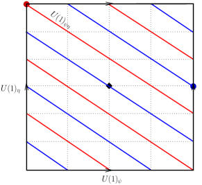
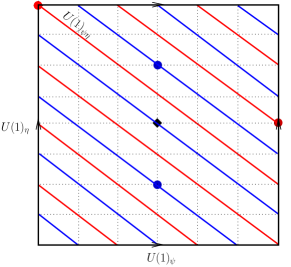
Figure 2: The torus $U(1)_{\psi}\times U(1)_{\eta}$ (for $N=2$ on the left and $N=4$ on the right) and its unbroken subgroup $U(1)_{\psi\eta}\times(\mathbbm{Z}_{2})_{F}$ (red line for $U(1)_{\psi\eta}\times\{1\}$ and blue line for $U(1)_{\psi\eta}\times\{-1\}$ ) passing through all the points of the lattice $(\mathbbm{Z}_{N+2})_{\psi}\times(\mathbbm{Z}_{N+4})_{\eta}$. The dots indicate the elements of the group $(\mathbbm{Z}_{N})$, diamonds indicate the elements of $(\mathbbm{Z}_{2})_{F}$. $(\mathbb{Z}_{2})_{F}$ is defined below, Eq. (29).

Let us consider the fermion parity defined by

$$\psi\to-\psi\;,\qquad\eta\to-\eta\;,$$ (29)

which is equivalent to a $2\pi$ space rotation. It is clear that $(\mathbb{Z}_{2})_{F}$ is not violated by the ’t Hooft vertex, so let us check if this is not a part of $U(1)_{\psi\eta}$. If it were included, there would be $\beta$ such that

$$\mathrm{e}^{\mathrm{i}{N+4\over 2}\beta}=\mathrm{e}^{-\mathrm{i}{N+2\over 2}\beta}=-1\;.$$ (30)

Multiplying these equations, we get $\mathrm{e}^{\mathrm{i}\beta}=1$, which is a contradiction.

It can be checked that any discrete transformation keeping ’t Hooft vertex invariant can be made of $U(1)_{\psi\eta}\times(\mathbb{Z}_{2})_{F}$. For example, $(\mathbb{Z}_{N+2})_{\psi}$ generated by $\psi\to\mathrm{e}^{\frac{2\pi\mathrm{i}}{N+2}}\psi$ can also be given by $\big{(}\beta=\frac{2\pi}{N+2},-1\big{)}\in U(1)_{\psi\eta}\times(\mathbb{Z}_{2})_{F}$. Similarly for $(\mathbb{Z}_{N+2})_{\eta}$.

For even $N$, we thus find that the symmetry group is

$$G_{\mathrm{f}}=\frac{U(1)_{\psi\eta}\times SU(N+4)\times(\mathbb{Z}_{2})_{F}}{\mathbb{Z}_{N}\times\mathbb{Z}_{N+4}}\;.$$ (31)

The division by $\mathbb{Z}_{N}$ in Eq. (31) is because the center of the color $SU(N)$ is shared by elements in $U(1)_{\psi\eta}\times(\mathbb{Z}_{2})_{F}$. Indeed, the gauge transformation with $\mathrm{e}^{\frac{2\pi\mathrm{i}}{N}}\in\mathbb{Z}_{N}\subset SU(N)$,

$$\psi\to\mathrm{e}^{\frac{4\pi\mathrm{i}}{N}}\psi\;,\;\qquad\eta\to\mathrm{e}^{-\frac{2\pi\mathrm{i}}{N}}\eta\;,$$ (32)

can be written equally well as the following $(\mathbb{Z}_{2})_{F}\times U(1)_{\psi\eta}$ transformation:

$$\psi\to(-1)\,\mathrm{e}^{\mathrm{i}{N+4\over 2}{2\pi\over N}}\psi=\mathrm{e}^{-\mathrm{i}{N\over 2}{2\pi\over N}}\,\mathrm{e}^{\mathrm{i}{N+4\over 2}{2\pi\over N}}\psi\;,\qquad\eta\to(-1)\,\mathrm{e}^{-\mathrm{i}{N+2\over 2}{2\pi\over N}}\eta=\mathrm{e}^{\mathrm{i}{N\over 2}{2\pi\over N}}\,\mathrm{e}^{-\mathrm{i}{N+2\over 2}{2\pi\over N}}\eta\;.$$ (33)

Note that the odd elements of $\mathbb{Z}_{N}$ belong to the disconnected component of $U(1)_{\psi\eta}\times(\mathbb{Z}_{2})_{F}$ while the even elements belong to the identity component.

The division by $\mathbb{Z}_{N+4}$ is understood in a similar manner. The center element $\mathrm{e}^{\frac{2\pi\mathrm{i}}{N+4}}\in SU(N+4)$ of the flavor group can be identified as the element of $U(1)_{\psi\eta}\times(\mathbb{Z}_{2})_{F}$ as follows:

$$\psi\to\psi=(-1)\,\mathrm{e}^{\mathrm{i}{N+4\over 2}{2\pi\over N+4}}\psi=\psi\;,\qquad\eta\to(-1)\,\mathrm{e}^{-\mathrm{i}{N+2\over 2}{2\pi\over N+4}}\eta=\mathrm{e}^{\mathrm{i}{2\pi\over N+4}}\eta\;.$$ (34)

Again, the odd elements of $\mathbb{Z}_{N+4}$ belong to the disconnected component of $U(1)_{\psi\eta}\times(\mathbb{Z}_{2})_{F}$ while the even elements belong to the identity component.

The anomaly-free symmetries and charges for various fields even $N$ are summarized in Table 3.

fields	$SU(N)_{\mathrm{c}}$	$SU(N+4)$	$U(1)_{\psi\eta}$	$({\mathbb{Z}}_{2})_{F}$
i $\psi$	${\yng(2)}$	$(\cdot)$	$\frac{N+4}{2}$	$+1$
$\eta$	$\bar{{\yng(1)}}$	${\yng(1)}$	$-\frac{N+2}{2}$	$-1$
$B^{AB}$	$(\cdot)$	${\yng(1,1)}$	$-\frac{N}{2}$	$-1$

Table 3: The charges of various fields with respect to the unbroken symmetry groups for even $N$. $B^{AB}$ are the possible massless composite fermion fields discussed in Sec. 2.1. The $({\mathbb{Z}}_{2})_{F}$ "charge" in the Table corresponds to the transformation $\psi\to e^{\mathrm{i}\pi}\psi$, $\eta\to e^{-\mathrm{i}\pi}\eta$.

3.3 Symmetry in the Higgs phase

In the Higgs phase the group (9) is actually a covering space of the true symmetry group which is given for any $N$ by

$$\frac{SU(N)_{\rm cf}\times SU(4)_{\rm f}\times U(1)^{\prime}\times(\mathbb{Z}_{2})_{F}}{\mathbbm{Z}_{N}\times\mathbbm{Z}_{4}}\;,$$ (35)

where $U(1)^{\prime}$ has charges given in Table 2. The fermion parity $(\mathbb{Z}_{2})_{F}$ is left unbroken by the condensate but is not contained in $U(1)^{\prime}$ so it must be kept in the numerator. The center of $SU(N)_{\rm cf}$ overlaps completely with $U(1)^{\prime}$ so it must be factorized (in fact we may write it as $U(N)_{\rm cf}$). The center of $SU(4)_{\rm f}$ also overlaps with $U(1)^{\prime}\times(\mathbb{Z}_{2})_{F}$ which explains the division by $\mathbbm{Z}_{4}$.

4 Mixed anomalies: Odd $N$ case

In this section we probe the system with a finer tool, i.e., by gauging possible 1-form center symmetries and studying possible mixed ’t Hooft anomalies, to see if a stronger constraint emerges. In order to detect the ’t Hooft anomalies, one needs to introduce the background gauge fields for the global symmetry $G_{\mathrm{f}}$, and check the violation of associated gauge invariance. Correspondingly to the symmetry of the system, Eq. (18), we thus introduce

• $A$: $U(1)_{\psi\eta}$ 1-form gauge field,

• $A_{\mathrm{f}}$: $SU(N+4)$ 1-form gauge field,

• $B^{(2)}_{\mathrm{c}}$: $\mathbb{Z}_{N}$ 2-form gauge field,

• $B^{(2)}_{\mathrm{f}}$: $\mathbb{Z}_{N+4}$ 2-form gauge field.

The field $A=A_{\mu}dx^{\mu}$ gauges the nonanomalous $U(1)_{\psi\eta}$ symmetry discussed in the previous subsection and the field $A_{\mathrm{f}}=A_{\mathrm{f}\,\mu}dx^{\mu}$ gauges the $SU(N+4)$ symmetry.

We recall that in order to gauge a $\mathbb{Z}_{n}$ discrete center symmetry of an $SU(n)$ theory, one introduces a pair of $U(1)$ gauge fields $\big{(}B^{(2)},B^{(1)}\big{)}$, 2-form and 1-form fields respectively, satisfying the constraint GKSW ; GKKS

$$nB^{(2)}={\mathrm{d}}B^{(1)}.$$ (36)

where $B^{(1)}$ satisfies

$$\frac{1}{2\pi}\int_{\Sigma_{2}}{\mathrm{d}}B^{(1)}={\mathbbm{Z}}\;.$$ (37)

Existence of the pair of gauge fields $\big{(}B^{(2)},B^{(1)}\big{)}$ satisfying relation (36) presumes one to have put the system in a topologically nontrivial spacetime $M$. In such a setting

$$e^{\mathrm{i}\int_{\Sigma_{2}}B^{(2)}}\in\,{\mathbbm{Z}}_{n}\;$$ (38)

corresponds to a nontrivial cocycle of $PSU(n)\equiv\frac{SU(n)}{{\mathbbm{Z}}_{n}}$ bundle: an elements of $w_{2}(M)\in H^{2}(M,{\mathbbm{Z}}_{n})$ known as the second Stiefel-Whitney class. The constraint (36) satisfies the invariance under the $U(1)$ 1-form gauge transformation,

$$B^{(2)}\to B^{(2)}+{\mathrm{d}}\lambda\;,\quad B^{(1)}\to B^{(1)}+n\lambda\;.$$ (39)

The idea is to couple these gauge fields appropriately to the standard gauge and matter fields, and to impose the invariance under the 1-form gauge transformation, Eq. (39), effectively yielding a $PSU(n)$ gauge theory.

This procedure will be applied below both to the color $SU(N)$ and flavor $SU(N+4)$ center symmetries. Actually, the whole analysis of this work could be performed, considering only the gauging of one of the 1-form symmetries, i.e., ${\mathbbm{Z}}_{N}$ or ${\mathbbm{Z}}_{N+4}$. In other words, one may set $B^{(2)}_{\mathrm{f}}=B^{(1)}_{\mathrm{f}}\equiv 0$, or $B^{(2)}_{\mathrm{c}}=B^{(1)}_{\mathrm{c}}\equiv 0$, throughout. We are free to choose which one of the 1-form global symmetries, or both, to gauge. In principle, the implication of our analysis may depend on such a choice. It turns out, however, that none of the main conclusions of this work (see Summary in Sec. 8) changes by keeping only one set of the two-form center gauge fields, ($B^{(2)}_{\mathrm{f}},B^{(1)}_{\mathrm{f}})$, or $(B^{(2)}_{\mathrm{c}},B^{(1)}_{\mathrm{c}})$, but this was not a priori known.

The $SU(N)$ dynamical gauge field $a$ is embedded into a $U(N)$ gauge field,

$$\widetilde{a}=a+{1\over N}B^{(1)}_{\mathrm{c}}\;,$$ (40)

and one requires invariance under $U(N)$ gauge transformations. Similarly, we introduce $U(N+4)$ gauge connection by

$$\widetilde{A}_{\mathrm{f}}=A_{\mathrm{f}}+{1\over N+4}B^{(1)}_{\mathrm{f}}\;,$$ (41)

and require $U(N+4)$ gauge invariance instead of the $SU(N+4)$ gauge invariance. The pairs of the 1-form$-$2-form $U(1)$ gauge fields are constrained as

$${N}B^{(2)}_{\mathrm{c}}=dB^{(1)}_{\mathrm{c}}\;,\qquad(N+4)B^{(2)}_{\mathrm{f}}=dB^{(1)}_{\mathrm{f}}\;.$$ (42)

The 1-form gauge transformations are defined by

$$B^{(2)}_{\mathrm{c}}\to B^{(2)}_{\mathrm{c}}+{\mathrm{d}}\lambda_{\mathrm{c}}\;,\qquad B^{(1)}_{\mathrm{c}}\to B^{(1)}_{\mathrm{c}}+{N}\lambda_{\mathrm{c}}\;,$$

$$B^{(2)}_{\mathrm{f}}\to B^{(2)}_{\mathrm{f}}+{\mathrm{d}}\lambda_{\mathrm{f}}\;,\qquad B^{(1)}_{\mathrm{f}}\to B^{(1)}_{\mathrm{f}}+(N+4)\lambda_{\mathrm{f}}\;;$$ (43)

$\lambda_{\mathrm{c}}$ and $\lambda_{\mathrm{f}}$ are $U(1)$ gauge fields. Under the $\mathbb{Z}_{N}$ and $\mathbb{Z}_{N+4}$ 1-form transformations, $U(N)$ and $U(N+4)$ transform as

$$\widetilde{a}\to\widetilde{a}+\lambda_{\mathrm{c}}\;,\qquad\widetilde{A}_{\mathrm{f}}\to\widetilde{A}_{\mathrm{f}}+\lambda_{\mathrm{f}}\;.$$ (44)

At the same time, $U(1)_{\psi\eta}$ gauge field is required to transform as

$$A\to A+{N-1\over 2}\lambda_{\mathrm{c}}+{N+3\over 2}\lambda_{\mathrm{f}}\;.$$ (45)

The transformation law for $A$ field is determined by the considerations made around Eqs. (20) and (21).

In order to have the invariance of the system under the 1-form gauge transformations the matter fermions must also be appropriately coupled to the 2-form gauge fields. Naively, the minimal coupling procedure gives the fermion kinetic term,

$$\overline{\psi}\gamma^{\mu}\Big{(}\partial+\mathcal{R}_{\mathrm{S}}(\widetilde{a})+(N+4)A\Big{)}_{\mu}P_{\mathrm{L}}\psi$$

$$+\,\overline{\eta}\gamma^{\mu}\left(\partial+\mathcal{R}_{\mathrm{F}^{*}}(\widetilde{a})+\widetilde{A}_{\mathrm{f}}-(N+2)A\right)_{\mu}P_{\mathrm{L}}\eta\;.$$ (46)

However, this is not invariant under (44)-(45). Indeed, the above combinations of gauge fields vary as

$$\delta\big{[}\mathcal{R}_{\mathrm{S}}(\widetilde{a})+(N+4)A\big{]} = {N+3\over 2}N\lambda_{\mathrm{c}}+{N+3\over 2}(N+4)\lambda_{\mathrm{f}}\;,$$

$$\delta\big{[}\mathcal{R}_{\mathrm{F}^{*}}(\widetilde{a})+\widetilde{A}_{\mathrm{f}}-(N+2)A\big{]} = -{N+1\over 2}N\lambda_{\mathrm{c}}-{N+1\over 2}(N+4)\lambda_{\mathrm{f}}\,.$$ (47)

We therefore require the correct fermion kinetic term with the background gauge fields to be

$$\overline{\psi}\gamma^{\mu}\left(\partial+\mathcal{R}_{\mathrm{S}}(\widetilde{a})+(N+4)A-{N+3\over 2}B^{(1)}_{\mathrm{c}}-{N+3\over 2}B^{(1)}_{\mathrm{f}}\right)_{\mu}P_{\mathrm{L}}\psi$$

$$+\,\overline{\eta}\gamma^{\mu}\left(\partial+\mathcal{R}_{\mathrm{F}^{*}}(\widetilde{a})+\widetilde{A}_{\mathrm{f}}-(N+2)A+{N+1\over 2}B^{(1)}_{\mathrm{c}}+{N+1\over 2}B^{(1)}_{\mathrm{f}}\right)_{\mu}P_{\mathrm{L}}\eta\;.$$ (48)

The two-index symmetric fermion $\psi$ feels the gauge field strength

$$\mathcal{R}_{\mathrm{S}}\big{(}F(\widetilde{a})\big{)}+(N+4){\mathrm{d}}A-{N(N+3)\over 2}B^{(2)}_{\mathrm{c}}-{(N+4)(N+3)\over 2}B^{(2)}_{\mathrm{f}}$$

$$=\mathcal{R}_{\mathrm{S}}\big{(}F(\tilde{a})-B^{(2)}_{\mathrm{c}}\big{)}+(N+4)\left[{\mathrm{d}}A-{N-1\over 2}B^{(2)}_{\mathrm{c}}-{N+3\over 2}B^{(2)}_{\mathrm{f}}\right]\;.$$ (49)

Note that the combination $F(\widetilde{a})-B^{(2)}_{\mathrm{c}}$ is traceless, hence an expression such as $\mathcal{R}_{\mathrm{S}}\big{(}F(\tilde{a})-B^{(2)}_{\mathrm{c}}\big{)}$ defined for an $SU(N)$ representation (in this particular case, a symmetric second-rank tensor representation) is well defined. Similarly, the anti-fundamental fermion $\eta$ feels the gauge field strength

$$\mathcal{R}_{\mathrm{F}^{*}}\big{(}F(\widetilde{a})\big{)}+F(\widetilde{A}_{\mathrm{f}})-(N+2){\mathrm{d}}A+{N(N-1)\over 2}B^{(2)}_{\mathrm{c}}+{(N+4)(N+1)\over 2}B^{(2)}_{\mathrm{f}}\qquad$$

$$=\mathcal{R}_{\mathrm{F}^{*}}\big{(}F(\widetilde{a})-B^{(2)}_{\mathrm{c}}\big{)}+\big{(}F(\widetilde{A}_{\mathrm{f}})-B^{(2)}_{\mathrm{f}}\big{)}-(N+2)\left[{\mathrm{d}}A-{N-1\over 2}B^{(2)}_{\mathrm{c}}-{N+3\over 2}B^{(2)}_{\mathrm{f}}\right]\;.$$

(50)

The low-energy "baryons" ${\cal B}^{[AB]}$ introduced in Eq. (7) for the chiral symmetric phase are described by the kinetic term,

$$\overline{\cal B}\,\gamma^{\mu}\left(\partial+\mathcal{R}_{A}(\widetilde{A}_{\mathrm{f}})-{N}A\right)_{\mu}P_{\mathrm{L}}{\cal B}\;,$$ (51)

yielding the 1-form gauge invariant form of the field tensor (see Eqs. (44)-(45)),

$$\mathcal{R}_{A}\big{(}F(\tilde{A_{\mathrm{f}}})-B^{(2)}_{\mathrm{f}}\big{)}-{N}\left[{\mathrm{d}}A-{N-1\over 2}B^{(2)}_{\mathrm{c}}-{N+3\over 2}B^{(2)}_{\mathrm{f}}\right]\;.$$ (52)

We are now ready to compute the anomalies following the standard Stora-Zumino descent procedure StoraZumino ; Zumino , as done also in Tanizaki . A good recent review of this renowned procedure can be found in 2groups . The contribution from $\psi$ to the $6D$ Abelian anomaly is

$${1\over 24\pi^{2}}\,{\mathrm{tr}}_{\mathcal{R}_{\mathrm{S}}}\left[\left\{\big{(}F(\tilde{a})-B^{(2)}_{\mathrm{c}}\big{)}+(N+4)\left[{\mathrm{d}}A-{N-1\over 2}B^{(2)}_{\mathrm{c}}-{N+3\over 2}B^{(2)}_{\mathrm{f}}\right]\right\}^{3}\right]$$

$$=\phantom{=}{N+4\over 24\pi^{2}}\,{\mathrm{tr}}\left[\big{(}F(\tilde{a})-B^{(2)}_{\mathrm{c}}\big{)}^{3}\right]$$

$$\phantom{=}+{(N+2)(N+4)\over 8\pi^{2}}\,{\mathrm{tr}}\left[\big{(}F(\tilde{a})-B^{(2)}_{\mathrm{c}}\big{)}^{2}\right]\wedge\left[{\mathrm{d}}A-{N-1\over 2}B^{(2)}_{\mathrm{c}}-{N+3\over 2}B^{(2)}_{\mathrm{f}}\right]$$

$$\phantom{=}+{N(N+1)\over 2}{(N+4)^{3}\over 24\pi^{2}}\left[{\mathrm{d}}A-{N-1\over 2}B^{(2)}_{\mathrm{c}}-{N+3\over 2}B^{(2)}_{\mathrm{f}}\right]^{3}\;.$$ (53)

When we write simply "${\mathrm{tr}}$" without an index the trace is taken in the fundamental representation. The contribution from $\eta$ is

$${1\over 24\pi^{2}}\,{\mathrm{tr}}\left(-[F(\widetilde{a})-B^{(2)}_{\mathrm{c}}]+[F(\widetilde{A}_{\mathrm{f}})-B^{(2)}_{\mathrm{f}}]-(N+2)\left[{\mathrm{d}}A-{N-1\over 2}B^{(2)}_{\mathrm{c}}-{N+3\over 2}B^{(2)}_{\mathrm{f}}\right]\right)^{3}$$

$$=-{(N+4)\over 24\pi^{2}}\,{\mathrm{tr}}\left[\big{(}F(\tilde{a})-B^{(2)}_{\mathrm{c}}\big{)}^{3}\right]$$

$$\phantom{=}-{(N+2)(N+4)\over 8\pi^{2}}\,{\mathrm{tr}}\left[\big{(}F(\tilde{a})-B^{(2)}_{\mathrm{c}}\big{)}^{2}\right]\wedge\left[{\mathrm{d}}A-{N-1\over 2}B^{(2)}_{\mathrm{c}}-{N+3\over 2}B^{(2)}_{\mathrm{f}}\right]$$

$$\phantom{=}+{N\over 24\pi^{2}}\,{\mathrm{tr}}\left[\big{(}F(\tilde{A}_{\mathrm{f}})-B^{(2)}_{\mathrm{f}}\big{)}^{3}\right]$$

$$\phantom{=}-{N(N+2)\over 8\pi^{2}}\,{\mathrm{tr}}\left[\big{(}F(\tilde{A}_{\mathrm{f}})-B^{(2)}_{\mathrm{f}}\big{)}^{2}\right]\wedge\left[{{\mathrm{d}}}A-{N-1\over 2}B^{(2)}_{\mathrm{c}}-{N+3\over 2}B^{(2)}_{\mathrm{f}}\right]$$

$$\phantom{=}-{N(N+4)(N+2)^{3}\over 24\pi^{2}}\left[{\mathrm{d}}A-{N-1\over 2}B^{(2)}_{\mathrm{c}}-{N+3\over 2}B^{(2)}_{\mathrm{f}}\right]^{3}.$$ (54)

By summing up these contributions, we obtain

$${N\over 24\pi^{2}}\,{\mathrm{tr}}\left[\big{(}F(\tilde{A}_{\mathrm{f}})-B^{(2)}_{\mathrm{f}}\big{)}^{3}\right]$$

$$-{N(N+2)\over 8\pi^{2}}\,{\mathrm{tr}}\left[\big{(}F(\tilde{A}_{\mathrm{f}})-B^{(2)}_{\mathrm{f}}\big{)}^{2}\right]\wedge\left[{\mathrm{d}}A-{N-1\over 2}B^{(2)}_{\mathrm{c}}-{N+3\over 2}B^{(2)}_{\mathrm{f}}\right]$$

$$-{(N+3)(N+4)\over 2}{N^{3}\over 24\pi^{2}}\left[{\mathrm{d}}A-{N-1\over 2}B^{(2)}_{\mathrm{c}}-{N+3\over 2}B^{(2)}_{\mathrm{f}}\right]^{3}\;.$$ (55)

Note that each factor in the square bracket in Eqs. (53)-(55) is 1-form gauge invariant.

By picking up the boundary terms one finds the $5D$ Wess-Zumino-Witten (WZW) action. For instance, in the limit the 1-form gauging is lifted (i.e., by setting $B^{(1)}_{\mathrm{f}}=B^{(1)}_{\mathrm{c}}=0$, $F(\tilde{A}_{\mathrm{f}})\to F({A}_{\mathrm{f}})$), one recovers, by using the identities

$${\mathrm{tr}}\big{(}F_{\mathrm{f}}^{2}\big{)}=d\,\Big{\{}{\mathrm{tr}}\big{(}A_{\mathrm{f}}dA_{\mathrm{f}}+\frac{2}{3}A_{\mathrm{f}}^{3}\big{)}\Big{\}}\;,\quad{\mathrm{tr}}\big{(}F_{\mathrm{f}}^{3}\big{)}=d\,\Big{\{}{\mathrm{tr}}\big{(}A_{\mathrm{f}}(dA_{\mathrm{f}})^{2}+\frac{3}{5}(A_{\mathrm{f}})^{5}+\frac{3}{2}A_{\mathrm{f}}^{3}dA_{\mathrm{f}}\big{)}\Big{\}}\;,$$ (56)

the well-known $5D$ action. The variations of the latter lead, by anomaly-inflow, to the famous $4D$ Abelian and nonAbelian anomaly expressions.

Note that the dependence on the color gauge field $\widetilde{a}$ disappeared from all terms. This is as it should be, for $N$ odd, as we are studying the ’t Hooft anomaly matching conditions for nonanomalous, continuous flavor symmetries.

As for the candidate massless "baryons" $\mathcal{B}$ the anomaly functional is given by

$${N+4-4\over 24\pi^{2}}\,{\mathrm{tr}}\left[\big{(}F(\tilde{A}_{\mathrm{f}})-B^{(2)}_{\mathrm{f}}\big{)}^{3}\right]$$

$$-{N(N+4-2)\over 8\pi^{2}}\,{\mathrm{tr}}\left[\big{(}F(\tilde{A}_{\mathrm{f}})-B^{(2)}_{\mathrm{f}}\big{)}^{2}\right]\wedge\left[{\mathrm{d}}A-{N-1\over 2}B^{(2)}_{\mathrm{c}}-{N+3\over 2}B^{(2)}_{\mathrm{f}}\right]$$

$$-{(N+3)(N+4)\over 2}{N^{3}\over 24\pi^{2}}\left[{\mathrm{d}}A-{N-1\over 2}B^{(2)}_{\mathrm{c}}-{N+3\over 2}B^{(2)}_{\mathrm{f}}\right]^{3}\;,$$ (57)

as can be seen easily from Eq. (52).

We are now in the position to compare the anomalies in the UV and IR. Somewhat surprisingly, we find that the IR anomalies Eq. (57) exactly reproduce the same $SU(N+4)\times U(1)_{\psi\eta}$ ’t Hooft anomalies of the UV theory Eq. (55), independently of whether or not the 2-form gauge fields $\big{(}B^{(2)}_{\mathrm{c}},B^{(2)}_{\mathrm{f}}\big{)}$ are introduced!

Actually, this is a simple consequence of the fact that without the 1-form gauging, these anomalies matched in the UV and IR (the earlier observation, see Sec. 2.1). The coefficients in various triangle diagrams involving $SU(N+4)$ and $U(1)_{\psi\eta}$ vertices, computed by using the UV and IR fermion degrees of freedom, are equal. Upon gauging the 1-form center symmetries, the external $SU(N+4)$ and $U(1)_{\psi\eta}$ gauge fields are replaced by the center-1-form-gauge-invariant combinations, both in the UV and IR, as in Eq. (49), Eq. (50), Eq. (52), but clearly the UV-IR matching of various anomalies continue to hold. It turns out that the situation is different when the UV-IR anomaly matching involves a discrete symmetry, as in even $N$ theories discussed below. See below.

5 Mixed anomalies: Even $N$ case

We discuss now the even $N$ theories. The calculation of the anomalies, 1-form gauging and anomaly matching checks go through mostly as in the odd $N$ case discussed above, by taking into account appropriately the difference in the $U(1)_{\psi\eta}$ charges of the matter fields and in the center symmetries themselves, as well as the presence of an independent discrete $({\mathbb{Z}}_{2})_{F}$ symmetry. However the conclusion turns out to be qualitatively different.

5.1 Calculation of anomalies

To detect the anomalies of global symmetry $G_{\mathrm{f}}$, Eq. (31), we introduce the gauge fields

• $A$: $U(1)_{\psi\eta}$ 1-form gauge field,

• $A_{2}^{(1)}$: $({\mathbb{Z}}_{2})_{F}$ 1-form gauge field,

• $A_{\mathrm{f}}$: $SU(N+4)$ 1-form gauge field,

• $B^{(2)}_{\mathrm{c}}$: $\mathbb{Z}_{N}$ 2-form gauge field,

• $B^{(2)}_{\mathrm{f}}$: $\mathbb{Z}_{N+4}$ 2-form gauge field.

$({\mathbb{Z}}_{2})_{F}$ is an ordinary ($0$-form) discrete symmetry, and we introduced accordingly a 1-form gauge field

$$A_{2}^{(1)}\;,\qquad\delta A_{2}^{(1)}=\frac{1}{2}\,\mathrm{d}\,\delta A_{2}^{(0)}\;.$$ (58)

The $({\mathbb{Z}}_{2})_{F}$ variation in the $4D$ action is described by,

$$\delta A_{2}^{(0)}=\pm 2\pi\;,\qquad{\rm i.e.}\;,\qquad\psi\to e^{\mathrm{i}\pi}\psi=-\psi,\quad\eta\to e^{-\mathrm{i}\pi}\eta=-\eta\;.$$ (59)

In order to avoid misunderstandings, let us repeat that $A_{2}^{(1)}$ is a gauge field formally introduced to describe an ordinary ($0$-form) $({\mathbb{Z}}_{2})_{F}$ symmetry. In this sense it is perfectly analogous to the $U(1)_{\psi\eta}$ gauge field, $A$. $\big{(}B_{\mathrm{c}}^{(2)}$, $B_{\mathrm{f}}^{(2)}\big{)}$ are instead introduced to "gauge" the 1-form center ($\mathbb{Z}_{N}$ and $\mathbb{Z}_{N+4}$) symmetries . The procedure was reviewed briefly at the beginning of Sec. 4, in the case of odd $N$ theories.

For even $N$ theories under consideration here, the construction is similar. We introduce two pairs of gauge fields $\big{(}B_{\mathrm{c}}^{(2)}$, $B_{\mathrm{c}}^{(1)}\big{)}$ and $\big{(}B_{\mathrm{f}}^{(2)}$, $B_{\mathrm{f}}^{(1)}\big{)}$, satisfying the constraints

$$NB_{\mathrm{c}}^{(2)}=dB_{\mathrm{c}}^{(1)}\;;\qquad(N+4)B_{\mathrm{f}}^{(2)}=dB_{\mathrm{f}}^{(1)}\;.$$ (60)

Under the gauged (1-form) center transformations, these fields transform as

$$B_{\mathrm{c}}^{(2)}\to B_{\mathrm{c}}^{(2)}+\mathrm{d}\lambda_{\mathrm{c}}\;,\qquad B_{\mathrm{c}}^{(1)}\to B_{\mathrm{c}}^{(1)}+N\lambda_{\mathrm{c}}\;,$$ (61)

$$B_{\mathrm{f}}^{(2)}\to B_{\mathrm{f}}^{(2)}+\mathrm{d}\lambda_{\mathrm{f}}\;,\qquad B_{\mathrm{f}}^{(1)}\to B_{\mathrm{f}}^{(1)}+(N+4)\lambda_{\mathrm{f}}\;,$$ (62)

which respect the constraints (60). Now the whole system must be made invariant under these transformations, and this requires the gauge fields $A$, $A_{2}$, $A_{\mathrm{f}}$, color $SU(N)$ gauge field $a$, as well as the fermions, be all coupled appropriately to $\big{(}B_{\mathrm{c}}^{(2)}$, $B_{\mathrm{c}}^{(1)}\big{)}$ and $\big{(}B_{\mathrm{f}}^{(2)}$, $B_{\mathrm{f}}^{(1)}\big{)}$ fields.

To achieve this we first embed the dynamical $SU(N)$ gauge field $a$ into a $U(N)$ gauge field $\widetilde{a}$ as

$$\widetilde{a}=a+{1\over N}B^{(1)}_{\mathrm{c}},$$ (63)

and the $SU(N+4)$ flavor gauge field as $U(N+4)$ gauge field $\widetilde{A}_{\mathrm{f}}$ as

$$\widetilde{A}_{\mathrm{f}}=A_{\mathrm{f}}+{1\over N+4}B^{(1)}_{\mathrm{f}}\,.$$ (64)

Under the center of $SU(N)$, the symmetry-group element $(\mathrm{e}^{\mathrm{i}\alpha},(-1)^{n},g_{\mathrm{f}})\in U(1)\times\mathbb{Z}_{2}\times SU(N+4)$ is identified as (see Eq. (33))

$$(\mathrm{e}^{\mathrm{i}\alpha},(-1)^{n},\,g_{\mathrm{f}})\sim(\mathrm{e}^{\mathrm{i}(\alpha-{2\pi\over N})},(-1)^{n}\mathrm{e}^{\mathrm{i}{2\pi\over N}{N\over 2}},\,g_{\mathrm{f}})\,.$$ (65)

This means that $U(1)_{\psi\eta}$ gauge field $A$ has charge $-1$, $(\mathbb{Z}_{2})_{F}$ gauge field $A_{2}^{(1)}$ has charge ${N\over 2}$, and $U(N+4)$ gauge field $\widetilde{A}_{\mathrm{f}}$ has charge $0$ under the $U(1)$ 1-form gauge transformation $\lambda_{\mathrm{c}}$ for $B_{\mathrm{c}}^{(2)}$.

Similarly, the division by $\mathbb{Z}_{N+4}$ means that we identify (see Eq. (34))

$$(\mathrm{e}^{\mathrm{i}\alpha},(-1)^{n},\,g_{\mathrm{f}})\sim(\mathrm{e}^{\mathrm{i}(\alpha-{2\pi\over N+4})},(-1)^{n}\mathrm{e}^{\mathrm{i}{N+4\over 2}{2\pi\over N+4}},\,g_{\mathrm{f}}\,\mathrm{e}^{2\pi\mathrm{i}\over N+4})\;,$$ (66)

and this determines the charges under $\lambda_{\mathrm{f}}$.

These considerations determine uniquely the way the 1-form gauge fields transform under (61) and (62):

$$\widetilde{a}\to\widetilde{a}+\lambda_{\mathrm{c}}\;,$$

$$A\to A-\lambda_{\mathrm{c}}-\lambda_{\mathrm{f}}\;,$$

$$A_{2}^{(1)}\to A_{2}^{(1)}+{N\over 2}\lambda_{\mathrm{c}}+{N+4\over 2}\lambda_{\mathrm{f}}\;,$$

$$\widetilde{A}_{\mathrm{f}}\to\widetilde{A}_{\mathrm{f}}+\lambda_{\mathrm{f}}\;.$$ (67)

The crucial ingredient in our analysis now is the nontrivial ’t Hooft fluxes carried by the (${\mathbbm{Z}}_{N}$ and ${\mathbbm{Z}}_{N+4}$) 2-form gauge fields $B_{\mathrm{c}}^{(2)}$ and $B_{\mathrm{f}}^{(2)}$,

$$\frac{1}{2\pi}\int_{\Sigma_{2}}B_{\mathrm{c}}^{(2)}=\frac{n_{1}}{N}\;,\qquad n_{1}\in{\mathbbm{Z}}_{N}\;,$$ (68)

$$\frac{1}{2\pi}\int_{\Sigma_{2}}B_{\mathrm{f}}^{(2)}=\frac{m_{1}}{N+4}\;,\qquad m_{1}\in{\mathbbm{Z}}_{N+4}\;,$$ (69)

in a closed two-dimensionl space, ${\Sigma_{2}}$. On topologically nontrivial four dimensional spacetime of Euclidean signature ${\Sigma_{2}}\times{\Sigma_{2}}$ one has then

$$\frac{1}{8\pi^{2}}\int_{\Sigma_{4}}(B_{\mathrm{c}}^{(2)})^{2}=\frac{n}{N^{2}}\;,\qquad\frac{1}{8\pi^{2}}\int_{\Sigma_{4}}(B_{\mathrm{f}}^{(2)})^{2}=\frac{m}{(N+4)^{2}}\;,$$ (70)

where $n\in{\mathbbm{Z}}_{N}$ and $m\in{\mathbbm{Z}}_{N+4}$, and an extra factor $2$ with respect to (68) is due to the two possible ways the two $B_{\mathrm{c}}^{(2)}$ fields are distributed on the two ${\Sigma_{2}}$’s (similarly for $B_{\mathrm{f}}^{(2)}$).

The fermion kinetic term with the background gauge field is obtained by the minimal coupling procedure as

$$\overline{\psi}\gamma^{\mu}\left(\partial+\mathcal{R}_{\mathrm{S}}(\widetilde{a})+{N+4\over 2}A+A_{2}\right)_{\mu}P_{\mathrm{L}}\psi\;$$

$$+\,\overline{\eta}\gamma^{\mu}\left(\partial+\mathcal{R}_{\mathrm{F}^{*}}(\widetilde{a})+\widetilde{A}_{\mathrm{f}}-{N+2\over 2}A-A_{2}\right)_{\mu}P_{\mathrm{L}}\eta\;.$$ (71)

Here, $A_{2}$ represents the coupling to the fermion parity $(-1)^{F}$, so its coefficient is meaningful only modulo $2$, and we fix the convention here. With this assignment of charges, each covariant derivative turns out to be invariant under 1-form gauge transformations without introducing extra terms. This is of course a direct reflection of the equivalence, (32) and (33), or (65), (66), i.e., of the requirement that the ${\mathbbm{Z}}_{N}\subset SU(N)$ transformation is canceled by $U(1)_{\psi\eta}\times{\mathbbm{Z}}_{2}$ (and similarly for the ${\mathbbm{Z}}_{N+4}$ symmetry).

We compute the anomalies again by applying the Stora-Zumino descent procedure starting with a $6D$ anomaly functional. The two-index symmetric fermion $\psi$ feels the gauge field strength

$$\mathcal{R}_{\mathrm{S}}\big{(}F(\widetilde{a})\big{)}+{N+4\over 2}{\mathrm{d}}A+\mathrm{d}A_{2} = \mathcal{R}_{\mathrm{S}}\big{(}F(\tilde{a})-B^{(2)}_{\mathrm{c}}\big{)}+{N+4\over 2}\left[{\mathrm{d}}A+B^{(2)}_{\mathrm{c}}+B^{(2)}_{\mathrm{f}}\right]$$ (72)

$$+\left[\mathrm{d}A_{2}^{(1)}-{N\over 2}B^{(2)}_{\mathrm{c}}-{N+4\over 2}B^{(2)}_{\mathrm{f}}\right]\;,$$

where appropriate 2-form gauge fields have been introduced so that each term is now 1-form gauge invariant. Similarly, the anti-fundamental fermion $\eta$ feels the gauge field strength

$$\mathcal{R}_{\mathrm{F}^{*}}\big{(}F(\widetilde{a})\big{)}+F(\widetilde{A}_{\mathrm{f}})-{N+2\over 2}{\mathrm{d}}A-\mathrm{d}A_{2}$$

$$=-[F(\widetilde{a})-B^{(2)}_{\mathrm{c}}]+[F(\widetilde{A}_{\mathrm{f}})-B^{(2)}_{\mathrm{f}}]-{N+2\over 2}\left[{\mathrm{d}}A+B^{(2)}_{\mathrm{c}}+B^{(2)}_{\mathrm{f}}\right]$$

$$\phantom{=}-\left[\mathrm{d}A_{2}^{(1)}-{N\over 2}B^{(2)}_{\mathrm{c}}-{N+4\over 2}B^{(2)}_{\mathrm{f}}\right]\;.$$ (73)

The low energy "baryons" gives

$$\mathcal{R}_{\mathrm{A}}\big{(}F(\widetilde{A}_{\mathrm{f}})\big{)}-{N\over 2}{\mathrm{d}}A-\mathrm{d}A_{2}$$

$$=\mathcal{R}_{\mathrm{A}}[F(\widetilde{A}_{\mathrm{f}})-B^{(2)}_{\mathrm{f}}]-{N\over 2}\left[{\mathrm{d}}A+B^{(2)}_{\mathrm{c}}+B^{(2)}_{\mathrm{f}}\right]-\left[\mathrm{d}A_{2}^{(1)}-{N\over 2}B^{(2)}_{\mathrm{c}}-{N+4\over 2}B^{(2)}_{\mathrm{f}}\right]\;.$$

(74)

Before proceeding to the calculation, let us make a brief pause. We have already noted that in contrast to the odd $N$ systems considered in Sec. 4, the fermion kinetic terms in an even $N$ theory (71) are invariant under the center gauge transformations, Eq. (61), Eq. (62), Eq. (67), without explicit addition of terms involving $B^{(2)}_{\mathrm{c}}$ and $B^{(2)}_{\mathrm{f}}$ (cfr. see Eq. (47) for the odd $N$ case). Thus the rewriting made above (72)-(74) might look redundant at first sight: these expressions appear to be actually independent of $B^{(2)}_{\mathrm{c}}$ and $B^{(2)}_{\mathrm{f}}$. This, however, is not quite correct. If one were to proceed with calculation without making each term 1-form gauge invariant, as done above, the resulting anomaly expressions would not be invariant under the 1-form ($\mathbb{Z}_{N}$ and $\mathbb{Z}_{N+4}$) center gauge transformations, so that there would be no guarantee that the mixed anomalies have been correctly evaluated in the reduced $PSU(N)$ or $PSU(N+4)$ theories. We thus prefer to work with explicitly 1-form gauge invariant forms at each step of the calculation below.

Let us proceed to the $6D$ anomaly functionals due to these fermions: $\psi$ gives, from Eq. (72),

$${1\over 24\pi^{2}}\,{\mathrm{tr}}\left(\mathcal{R}_{\mathrm{S}}\big{(}F(\tilde{a})-B^{(2)}_{\mathrm{c}}\big{)}+{N+4\over 2}\left[{\mathrm{d}}A+B^{(2)}_{\mathrm{c}}+B^{(2)}_{\mathrm{f}}\right]\right.$$

$$\qquad\qquad\ \left.+\left[\mathrm{d}A_{2}^{(1)}-{N\over 2}B^{(2)}_{\mathrm{c}}-{N+4\over 2}B^{(2)}_{\mathrm{f}}\right]\right)^{3}$$

$$=\phantom{=}{(N+4)\over 24\pi^{2}}\,\mathrm{tr}\left[\big{(}F(\tilde{a})-B^{(2)}_{\mathrm{c}}\big{)}^{3}\right]$$

$$\phantom{=}+{(N+2)(N+4)\over 16\pi^{2}}\,\mathrm{tr}\left[\big{(}F(\tilde{a})-B^{(2)}_{\mathrm{c}}\big{)}^{2}\right]\wedge\left[{\mathrm{d}}A+B^{(2)}_{\mathrm{c}}+B^{(2)}_{\mathrm{f}}\right]$$

$$\phantom{=}+\frac{N(N+1)}{2\cdot 24\pi^{2}}\left(\frac{N+4}{2}\right)^{3}\left[{\mathrm{d}}A+B^{(2)}_{\mathrm{c}}+B^{(2)}_{\mathrm{f}}\right]^{3}$$

$$\phantom{=}+\frac{N+2}{8\pi^{2}}\,{\mathrm{tr}}\big{(}F(\tilde{a})-B^{(2)}_{\mathrm{c}}\big{)}^{2}\left[\mathrm{d}A_{2}^{(1)}-{N\over 2}B^{(2)}_{\mathrm{c}}-{N+4\over 2}B^{(2)}_{\mathrm{f}}\right]$$

$$\phantom{=}+\frac{1}{8\pi^{2}}\left(\frac{N+4}{2}\right)^{2}\frac{N(N+1)}{2}\left[{\mathrm{d}}A+B^{(2)}_{\mathrm{c}}+B^{(2)}_{\mathrm{f}}\right]^{2}\left[\mathrm{d}A_{2}^{(1)}-{N\over 2}B^{(2)}_{\mathrm{c}}-{N+4\over 2}B^{(2)}_{\mathrm{f}}\right]$$

$$\phantom{=}+\frac{1}{8\pi^{2}}\left(\frac{N+4}{2}\right)\frac{N(N+1)}{2}\left[{\mathrm{d}}A+B^{(2)}_{\mathrm{c}}+B^{(2)}_{\mathrm{f}}\right]\left[\mathrm{d}A_{2}^{(1)}-{N\over 2}B^{(2)}_{\mathrm{c}}-{N+4\over 2}B^{(2)}_{\mathrm{f}}\right]^{2}$$

$$\phantom{=}+{1\over 24\pi^{2}}\frac{N(N+1)}{2}\left[\mathrm{d}A_{2}^{(1)}-{N\over 2}B^{(2)}_{\mathrm{c}}-{N+4\over 2}B^{(2)}_{\mathrm{f}}\right]^{3}\;.$$ (75)

The contribution of $\eta$ is (from Eq. (73)):

$${1\over 24\pi^{2}}\,{\mathrm{tr}}\,{\huge\{}-[F(\widetilde{a})-B^{(2)}_{\mathrm{c}}]+[F(\widetilde{A}_{\mathrm{f}})-B^{(2)}_{\mathrm{f}}]-{N+2\over 2}\left[{\mathrm{d}}A+B^{(2)}_{\mathrm{c}}+B^{(2)}_{\mathrm{f}}\right]$$

$$-\left[\mathrm{d}A_{2}^{(1)}-{N\over 2}B^{(2)}_{\mathrm{c}}-{N+4\over 2}B^{(2)}_{\mathrm{f}}\right]{\huge\}}^{3}$$

$$=-{(N+4)\over 24\pi^{2}}\,\mathrm{tr}\left[\big{(}F(\tilde{a})-B^{(2)}_{\mathrm{c}}\big{)}^{3}\right]+{N\over 24\pi^{2}}\mathrm{tr}\left[\big{(}F(\tilde{A}_{\mathrm{f}})-B^{(2)}_{\mathrm{f}}\big{)}^{3}\right]$$

$$\phantom{=}-{(N+2)(N+4)\over 16\pi^{2}}\,\mathrm{tr}\left[\big{(}F(\tilde{a})-B^{(2)}_{\mathrm{c}}\big{)}^{2}\right]\wedge\left[{\mathrm{d}}A+B^{(2)}_{\mathrm{c}}+B^{(2)}_{\mathrm{f}}\right]$$

$$\phantom{=}-\frac{N}{8\pi^{2}}\frac{N+2}{2}\,{\mathrm{tr}}[F(\widetilde{A}_{\mathrm{f}})-B^{(2)}_{\mathrm{f}}]^{2}\left[{\mathrm{d}}A+B^{(2)}_{\mathrm{c}}+B^{(2)}_{\mathrm{f}}\right]$$

$$\phantom{=}-{N(N+4)(N+2)^{3}\over 8\cdot 24\pi^{2}}\left[{\mathrm{d}}A+B^{(2)}_{\mathrm{c}}+B^{(2)}_{\mathrm{f}}\right]^{3}$$

$$\phantom{=}-\frac{N+4}{8\pi^{2}}\,{\mathrm{tr}}\big{(}F(\tilde{a})-B^{(2)}_{\mathrm{c}}\big{)}^{2}\left[\mathrm{d}A_{2}^{(1)}-{N\over 2}B^{(2)}_{\mathrm{c}}-{N+4\over 2}B^{(2)}_{\mathrm{f}}\right]$$

$$\phantom{=}-\frac{N}{8\pi^{2}}\,{\mathrm{tr}}[F(\widetilde{A}_{\mathrm{f}})-B^{(2)}_{\mathrm{f}}]^{2}\left[\mathrm{d}A_{2}^{(1)}-{N\over 2}B^{(2)}_{\mathrm{c}}-{N+4\over 2}B^{(2)}_{\mathrm{f}}\right]$$

$$\phantom{=}-\frac{1}{8\pi^{2}}\left(\frac{N+2}{2}\right)^{2}N(N+4)\left[{\mathrm{d}}A+B^{(2)}_{\mathrm{c}}+B^{(2)}_{\mathrm{f}}\right]^{2}\left[\mathrm{d}A_{2}^{(1)}-{N\over 2}B^{(2)}_{\mathrm{c}}-{N+4\over 2}B^{(2)}_{\mathrm{f}}\right]$$

$$\phantom{=}-\frac{1}{8\pi^{2}}\left(\frac{N+2}{2}\right)N(N+4)\left[{\mathrm{d}}A+B^{(2)}_{\mathrm{c}}+B^{(2)}_{\mathrm{f}}\right]\left[\mathrm{d}A_{2}^{(1)}-{N\over 2}B^{(2)}_{\mathrm{c}}-{N+4\over 2}B^{(2)}_{\mathrm{f}}\right]^{2}$$

$$\phantom{=}-{1\over 24\pi^{2}}N(N+4)\left[\mathrm{d}A_{2}^{(1)}-{N\over 2}B^{(2)}_{\mathrm{c}}-{N+4\over 2}B^{(2)}_{\mathrm{f}}\right]^{3}\;.$$ (76)

The sum of the UV anomalies is

$$+{N\over 24\pi^{2}}\mathrm{tr}\left[\big{(}F(\tilde{A}_{\mathrm{f}})-B^{(2)}_{\mathrm{f}}\big{)}^{3}\right]$$

$$-\frac{N}{8\pi^{2}}\frac{N+2}{2}{\mathrm{tr}}[F(\widetilde{A}_{\mathrm{f}})-B^{(2)}_{\mathrm{f}}]^{2}\left[{\mathrm{d}}A+B^{(2)}_{\mathrm{c}}+B^{(2)}_{\mathrm{f}}\right]$$

$$-{N^{3}(N+4)(N+3)\over 16\cdot 24\pi^{2}}\left[{\mathrm{d}}A+B^{(2)}_{\mathrm{c}}+B^{(2)}_{\mathrm{f}}\right]^{3}$$

$$-\frac{2}{8\pi^{2}}{\mathrm{tr}}\big{(}F(\tilde{a})-B^{(2)}_{\mathrm{c}}\big{)}^{2}\left[\mathrm{d}A_{2}^{(1)}-{N\over 2}B^{(2)}_{\mathrm{c}}-{N+4\over 2}B^{(2)}_{\mathrm{f}}\right]$$

$$-\frac{N}{8\pi^{2}}{\mathrm{tr}}[F(\widetilde{A}_{\mathrm{f}})-B^{(2)}_{\mathrm{f}}]^{2}\left[\mathrm{d}A_{2}^{(1)}-{N\over 2}B^{(2)}_{\mathrm{c}}-{N+4\over 2}B^{(2)}_{\mathrm{f}}\right]$$

$$-\frac{1}{8\pi^{2}}\frac{N(N+4)(N^{2}+3N+4)}{8}\left[{\mathrm{d}}A+B^{(2)}_{\mathrm{c}}+B^{(2)}_{\mathrm{f}}\right]^{2}\left[\mathrm{d}A_{2}^{(1)}-{N\over 2}B^{(2)}_{\mathrm{c}}-{N+4\over 2}B^{(2)}_{\mathrm{f}}\right]$$

$$-\frac{1}{8\pi^{2}}\frac{N(N+3)(N+4)}{4}\left[{\mathrm{d}}A+B^{(2)}_{\mathrm{c}}+B^{(2)}_{\mathrm{f}}\right]\left[\mathrm{d}A_{2}^{(1)}-{N\over 2}B^{(2)}_{\mathrm{c}}-{N+4\over 2}B^{(2)}_{\mathrm{f}}\right]^{2}$$

$$-{1\over 24\pi^{2}}\frac{N(N+7)}{2}\left[\mathrm{d}A_{2}^{(1)}-{N\over 2}B^{(2)}_{\mathrm{c}}-{N+4\over 2}B^{(2)}_{\mathrm{f}}\right]^{3}\;.$$ (77)

In the IR, the "baryons" Eq. (7) yield, from Eq. (74), the $6D$ anomaly

$${1\over 24\pi^{2}}\,{\mathrm{tr}}\left(\mathcal{R}_{\mathrm{A}}(F(\widetilde{A}_{\mathrm{f}})-B^{(2)}_{\mathrm{f}})-{N\over 2}\left[{\mathrm{d}}A+B^{(2)}_{\mathrm{c}}+B^{(2)}_{\mathrm{f}}\right]\right.$$

$$\qquad\qquad\ \left.-\left[\mathrm{d}A_{2}^{(1)}-{N\over 2}B^{(2)}_{\mathrm{c}}-{N+4\over 2}B^{(2)}_{\mathrm{f}}\right]\right)^{3}$$

$$=\phantom{=}{N+4-4\over 24\pi^{2}}\mathrm{tr}\left[\big{(}F(\tilde{A}_{\mathrm{f}})-B^{(2)}_{\mathrm{f}}\big{)}^{3}\right]$$

$$\phantom{=}-{N^{3}(N+4)(N+3)\over 16\cdot 24\pi^{2}}\left[{\mathrm{d}}A+B^{(2)}_{\mathrm{c}}+B^{(2)}_{\mathrm{f}}\right]^{3}$$

$$\phantom{=}-\frac{N+2}{8\pi^{2}}\frac{N}{2}{\mathrm{tr}}[F(\widetilde{A}_{\mathrm{f}})-B^{(2)}_{\mathrm{f}}]^{2}\left[{\mathrm{d}}A+B^{(2)}_{\mathrm{c}}+B^{(2)}_{\mathrm{f}}\right]$$

$$\phantom{=}-\frac{N+2}{8\pi^{2}}{\mathrm{tr}}[F(\widetilde{A}_{\mathrm{f}})-B^{(2)}_{\mathrm{f}}]^{2}\left[\mathrm{d}A_{2}^{(1)}-{N\over 2}B^{(2)}_{\mathrm{c}}-{N+4\over 2}B^{(2)}_{\mathrm{f}}\right]$$

$$\phantom{=}-\frac{1}{8\pi^{2}}\left(\frac{N}{2}\right)^{2}\frac{(N+4)(N+3)}{2}\left[{\mathrm{d}}A+B^{(2)}_{\mathrm{c}}+B^{(2)}_{\mathrm{f}}\right]^{2}\left[\mathrm{d}A_{2}^{(1)}-{N\over 2}B^{(2)}_{\mathrm{c}}-{N+4\over 2}B^{(2)}_{\mathrm{f}}\right]$$

$$\phantom{=}-\frac{1}{8\pi^{2}}\frac{N}{2}\frac{(N+4)(N+3)}{2}\left[{\mathrm{d}}A+B^{(2)}_{\mathrm{c}}+B^{(2)}_{\mathrm{f}}\right]\left[\mathrm{d}A_{2}^{(1)}-{N\over 2}B^{(2)}_{\mathrm{c}}-{N+4\over 2}B^{(2)}_{\mathrm{f}}\right]^{2}$$

$$\phantom{=}-{1\over 24\pi^{2}}\frac{(N+4)(N+3)}{2}\left[\mathrm{d}A_{2}^{(1)}-{N\over 2}B^{(2)}_{\mathrm{c}}-{N+4\over 2}B^{(2)}_{\mathrm{f}}\right]^{3}\;.$$ (78)

Note that the second-from-the-last term, corresponding to $[{\mathbbm{Z}}_{2}]^{2}-U(1)_{\psi\eta}$ anomaly, is identical in the UV and in the IR, see Eq. (77) and Eq. (78).

5.2 An almost flat $({\mathbbm{Z}}_{2})_{F}$ connection, generalized cocycle condition, and the ’t Hooft fluxes

Before proceeding to the actual determination of various mixed anomalies, let us recapitulate some formal points involved in our analysis. The first is the meaning of the gauge field for $({\mathbbm{Z}}_{2})_{F}$ introduced above. The combination

$$2A_{2}^{(1)}-B^{(1)}_{\mathrm{c}}-B^{(1)}_{\mathrm{f}}=dA_{2}^{(0)}\;,$$ (79)

is the modification of the $({\mathbbm{Z}}_{2})_{F}$ gauge field, $2A_{2}^{(1)}=dA_{2}^{(0)}$, such that it is invariant under the 1-form gauge transformations, (61)-(67). By taking the derivatives of the both sides of Eq. (79) it might appear that one gets

$$2\,\mathrm{d}A_{2}^{(1)}-{N}B^{(2)}_{\mathrm{c}}-(N+4)B^{(2)}_{\mathrm{f}}=0\;:$$ (80)

this would erase all terms containing $2\,\mathrm{d}A_{2}^{(1)}-{N}B^{(2)}_{\mathrm{c}}-(N+4)B^{(2)}_{\mathrm{f}}$ from the $6D$ action, (75)-(78). This, of course, is not correct as $A_{2}^{(0)}$ is a $2\pi$ periodic (angular) field. Indeed, the left hand side of Eq. (79) is "an almost flat connection": Eq. (80) is correct locally, but cannot be set to zero identically, as it can give nontrivial contribution when integrated over $\Sigma_{2}$.

Actually, by integrating the both sides of Eq. (79) over a noncontractible cycle, one gets

$$\oint dx^{\mu}\big{(}2A_{2}^{(1)}-B^{(1)}_{\mathrm{c}}-B^{(1)}_{\mathrm{f}}\big{)}_{\mu}=\oint dA_{2}^{(0)}=2\pi n\;,\qquad n\in{\mathbbm{Z}}\;,$$

$$\oint A_{2}^{(1)}=\frac{2\pi m}{2}\;,\qquad m\in{\mathbbm{Z}}\;,$$ (81)

and

$$\int_{\Sigma_{2}}N\,B^{(2)}_{\mathrm{c}}+\int_{\Sigma_{2}}(N+4)\,B^{(2)}_{\mathrm{f}}=2\pi k\;,\qquad k\in{\mathbbm{Z}}\;,$$ (82)

where $\Sigma_{2}$ is taken to be a nontrivial closed two-dimensional surface. Eq. (81) is a trademark of a $\mathbbm{Z}_{2}$ gauge field. Eq. (82) is consistent with mutually independent fluxes of $B^{(2)}_{\mathrm{c}}$ and $B^{(2)}_{\mathrm{f}}$, (68)-(70). In passing, we note that this is in line with the remark made in Sec. 4, that the whole analysis of this work could have been done possibly by keeping only one of the 2-form gauge fields, $B^{(2)}_{\mathrm{c}}$ or $B^{(2)}_{\mathrm{f}}$.

All this can be rephrased in terms of the generalized cocycle. In the case of standard QCD with massless left-handed and right-handed quarks, the relevant symmetry involves ${\mathbbm{Z}}_{N}\subset SU(N)_{\mathrm{c}}$ and ${\mathbbm{Z}}_{N}\subset U(1)_{V}$. By compensating the failure of the cocycle condition at a triple overlap region of spacetime manifold by a color ${\mathbbm{Z}}_{N}$ factor by a simultaneous ${\mathbbm{Z}}_{N}\subset U(1)_{V}$ transformation, one can formulate a consistent $\frac{SU(N)}{{\mathbbm{Z}}_{N}}$ "QCD".

In our case, the failure of the straightforward cocycle condition by color ${\mathbbm{Z}}_{N}$ center factor can be compensated by a simultaneous ${\mathbbm{Z}}_{N}\subset U(1)_{\psi\eta}\times{\mathbbm{Z}}_{2}$ phase transformation of the fermions. See Eq. (32) and Eq. (33). Similarly for the ${\mathbbm{Z}}_{N+4}$ center. The consistency for $\psi$ and $\eta$ gauge transformations in a triple overlapping region thus reads

$$\left(e^{\mathrm{i}\tfrac{2\pi}{N}n_{ij}}\right)^{2}=\mp e^{-\mathrm{i}\tfrac{N+4}{2}\Delta\alpha_{ij}}\;,$$ (83)

and

$$\left(e^{\mathrm{i}\tfrac{2\pi}{N}n_{ij}}\right)^{-1}e^{\tfrac{2\pi\mathrm{i}}{N+4}m_{ij}}=\mp e^{\mathrm{i}\tfrac{N+2}{2}\Delta\alpha_{ij}}\;,$$ (84)

respectively. Finding $e^{\mathrm{i}\Delta\alpha_{ij}}$ by multiplying Eq. (83) and Eq. (84) and inserting it back, one gets a consistency condition

$$e^{\pi\mathrm{i}(n_{ij}+m_{ij})}=\mp 1\;.$$ (85)

If (83) and (84) were to be interpreted in terms of ’t Hooft’s twisted periodic conditions, the exponents in these formulas, $\tfrac{2\pi}{N}n_{ij}$, $\tfrac{2\pi}{N+4}m_{ij}$, $\pm\pi$, $\Delta\alpha_{ij}$ would respectively be the $SU(N)$, $SU(N+4)$, $({\mathbbm{Z}}_{2})_{F}$ and $U_{\psi\eta}(1)$ fluxes through a closed two dimensional surface, $\Sigma_{2}$. This requires some care, because of the discrete periodicity of the $({\mathbbm{Z}}_{2})_{F}$ gauge field. In particular the presence of such a flux means that, if $\Sigma_{2}$ is taken as a torus, there should be a point-like singularity on it (2-dimensional surfaces, from the point of view of the four dimensional spacetime), carrying a $(\mathbbm{Z}_{2})_{F}$ flux. Actually, it seems to us more natural, in the presence of a $(\mathbbm{Z}_{2})_{F}$ gauge field, to take as $\Sigma_{2}$ not a torus with a singularity, but a smooth Riemann surface of genus $2$ (a double torus).

As already noted in Sec. 4, these indices $n_{ij}$ (or $m_{ij}$) correspond exactly to the second Stiefel-Whitney class of $\frac{SU(N)}{{\mathbbm{Z}}_{N}}$ (or $\frac{SU(N+4)}{{\mathbbm{Z}}_{N+4}}$) connections. In other words, the condition (85) translates into the $B^{(2)}_{\mathrm{c}}$ and $B^{(2)}_{\mathrm{f}}$ flux relation, Eq. (82).

5.3 Anomaly matching without the gauging of the 1-form center symmetries

As another little preparation for our calculations, let us first check that our gauge fields and their variations are properly normalized, by considering the anomalies in the ordinary case, i.e., where the 1-form ${\mathbbm{Z}}_{N}$ and ${\mathbbm{Z}}_{N+4}$ symmetries are not gauged. In other words, we set

$$B^{(2)}_{\mathrm{c}}=B^{(1)}_{\mathrm{c}}=B^{(2)}_{\mathrm{f}}=B^{(1)}_{\mathrm{f}}=0\;.$$ (86)

The first three terms (the triangles involving $U(1)_{\psi\eta}$ and $SU(N+4)$) of Eq. (78) match exactly those in the UV anomaly, Eq. (77), whether or not $\big{(}B^{(2)}_{\mathrm{c}}\,,B^{(2)}_{\mathrm{f}}\big{)}$ fields are present. The second-from-the-last terms in Eq. (77) and in Eq. (78) describe the nontrivial $[({\mathbbm{Z}}_{2})_{F}]^{2}-U(1)_{\psi\eta}$ anomaly, which are identical in UV and IR, again, whether or not the 1-form gauging of ${\mathbbm{Z}}_{N}$ and ${\mathbbm{Z}}_{N+4}$ is done.

To compute the $({\mathbbm{Z}}_{2})_{F}$ anomaly in the UV, one collects the terms

$$\int_{\Sigma_{6}}(\ldots)\,\mathrm{d}A_{2}^{(1)}\;,$$ (87)

and integrate to get the boundary $5D$ effective WZW action

$$\int_{\Sigma_{5}}(\ldots)\,A_{2}^{(1)}\;.$$ (88)

The $({\mathbbm{Z}}_{2})_{F}$ transformations of the fermions are formally expressed as the transformation of the $({\mathbbm{Z}}_{2})_{F}$ "gauge field" $A_{2}^{(1)}$,

$$A_{2}^{(1)}\to A_{2}^{(1)}+\frac{1}{2}\,d(\delta A_{2}^{(0)})\;,\qquad\delta A_{2}^{(0)}=\pm 2\pi\;,$$ (89)

yielding the anomaly-inflow in $4D$

$$\delta S^{4}_{\rm UV} = -\frac{2}{8\pi^{2}}\int_{\Sigma_{4}}{\mathrm{tr}}[F({a})]^{2}\,\frac{\delta A_{2}^{(0)}}{2}-\frac{N}{8\pi^{2}}\int_{\Sigma_{4}}{\mathrm{tr}}[F({A}_{\mathrm{f}})]^{2}\,\frac{\delta A_{2}^{(0)}}{2}$$ (90)

$$-\frac{1}{8\pi^{2}}\frac{N(N+4)(N^{2}+3N+4)}{8}\int_{\Sigma_{4}}\left[{\mathrm{d}}A\right]^{2}\,\frac{\delta A_{2}^{(0)}}{2}\;.$$

The first line is the standard chiral anomaly expression associated with the field transformation

$$\psi\to-\psi\;,\qquad\eta\to-\eta\;,\qquad\delta A_{2}^{(0)}=\pm 2\pi\;$$ (91)

due to $SU(N)$ and $SU(N+4)$ gauge fields. They are actually both trivial (no anomalies) due to the integer instanton numbers:

$$\frac{1}{8\pi^{2}}\int_{\Sigma_{4}}{\mathrm{tr}}[F(a)]^{2}=\mathbbm{Z}\;,\qquad\frac{1}{8\pi^{2}}\int_{\Sigma_{4}}{\mathrm{tr}}[F({A}_{\mathrm{f}})]^{2}=\mathbbm{Z}\;.$$ (92)

Note that, crucially, their coefficients ($2$ and $N$) are both even integers. This confirms that the field $A_{2}^{(1)}$ and its variation $\delta A_{2}^{(0)}$ are correctly normalized.

Similarly in the IR one has

$$\Delta S^{4}_{\rm IR} = -\frac{N+2}{8\pi^{2}}\int{\mathrm{tr}}[F({A}_{\mathrm{f}})]^{2}\,\frac{\delta A_{2}^{(0)}}{2}$$ (93)

$$-\frac{1}{8\pi^{2}}\left(\frac{N}{2}\right)^{2}\frac{(N+4)(N+3)}{2}\int\left[{\mathrm{d}}A\right]^{2}\,\frac{\delta A_{2}^{(0)}}{2}\;.$$

Again, the first term is trivial, as $N+2$ is an even integer.

The second terms in Eq. (90) and in Eq. (93) describe the nontrivial $({\mathbbm{Z}}_{2})_{F}-[U(1)_{\psi\eta}]^{2}$ anomaly, present both in the UV and in the IR. However, their difference is given by

$$-\frac{N(N+4)}{2}\int\left(\frac{1}{8\pi^{2}}\left[{\mathrm{d}}A\right]^{2}\right)\cdot\,\frac{\delta A_{2}^{(0)}}{2}\;.$$ (94)

Since the coefficient $\frac{N(N+4)}{2}$ is any even integer the discrete $({\mathbbm{Z}}_{2})_{F}-[U(1)_{\psi\eta}]^{2}$ anomaly is matched modulo ${\mathbbm{Z}}_{2}$ in the IR and UV.

All in all, we reproduce the earlier results reported in Sec. 2, that a chirally symmetric vacuum, with no condensates, with no NG bosons but with massless baryons Eq. (7), satisfy all the conventional ’t Hooft anomaly matching constraints.

6 UV-IR matching of various mixed anomalies in even $N$ theories

Now we come to the main issues of our analysis: studying the various mixed anomalies involving the fermion parity $({\mathbbm{Z}}_{2})_{F}$, in the presence of the 2-form gauge fields $B^{(2)}_{\mathrm{c}}$ and $B^{(2)}_{\mathrm{f}}$, in an even $N$ theory. Starting from the $6D$ action, Eq. (75) - Eq. (78), one collects the terms of the form,

$$S^{6D}=\int_{6}\,[...]\,\left[\mathrm{d}A_{2}^{(1)}-{N\over 2}B^{(2)}_{\mathrm{c}}-{N+4\over 2}B^{(2)}_{\mathrm{f}}\right]\;.$$ (95)

Integrating, one gets the 5D boundary WZW action

$$S^{5D}=\int_{5}\,[...]\,\left[A_{2}^{(1)}-\frac{1}{2}B^{(1)}_{\mathrm{c}}-\frac{1}{2}B^{(1)}_{\mathrm{f}}\right]\;.$$ (96)

This allows us to calculate various anomalies in $4D$ involving $({\mathbbm{Z}}_{2})_{F}$, by anomaly inflow, considering the variations

$$\delta[A_{2}^{(1)}-\frac{1}{2}B^{(1)}_{\mathrm{c}}-\frac{1}{2}B^{(1)}_{\mathrm{f}}]=\frac{1}{2}\,\mathrm{d}\,\delta A_{2}^{(0)}\;,$$ (97)

$$\delta S^{4D}=\frac{1}{2}\int_{4}\,[...]\,\delta A_{2}^{(0)}\;,\qquad\delta A_{2}^{(0)}=\pm 2\pi\,.$$ (98)

6.1 Mixed $({\mathbb{Z}}_{2})_{F}-[\mathbb{Z}_{N}]^{2}$ anomaly

Collecting all terms of the form

$$N^{2}\int(B^{(2)}_{\mathrm{c}})^{2}A_{2}^{(1)}$$ (99)

in the $5D$ WZW action, one finds at UV,

$$S^{(5)}_{\rm UV}=1\cdot\frac{1}{8\pi^{2}}\int_{\Sigma_{5}}N^{2}(B^{(2)}_{\mathrm{c}})^{2}\cdot A_{2}^{(1)}\;.$$ (100)

The coefficient in front of the above expression (100) is the result of the sum from various $\psi$ and $\eta$ contributions in (75) and (76):

$$-\frac{N+2}{N}+\frac{(N+1)(N+4)^{2}}{8N}-\frac{(N+4)(N+1)}{4}+\frac{N(N+1)}{8}$$

$$+\frac{N+4}{N}-\frac{(N+4)(N+2)^{2}}{4N}+\frac{(N+2)(N+4)}{2}-\frac{N(N+4)}{4}=1\;.$$ (101)

The result (100) leads to the $4D$ mixed $({\mathbb{Z}}_{2})_{F}-[\mathbb{Z}_{N}]^{2}$ anomaly in the UV,

$$\Delta S^{(4)}_{\rm UV}=\pm\mathrm{i}\pi{\mathbbm{Z}}\;,\qquad\delta A_{2}^{(1)}=d\,\frac{1}{2}\delta A_{2}^{(0)}\;,\qquad\delta A_{2}^{(0)}=\pm 2\pi\,.$$ (102)

In other words, the partition function changes sign under the ${\mathbbm{Z}}_{2}$ transformation, $\psi\to-\psi$, $\eta\to-\eta$, in appropriate background $B^{(2)}_{\mathrm{c}}$ fields

$$\frac{1}{8\pi^{2}}\int_{\Sigma_{4}}N^{2}(B^{(2)}_{\mathrm{c}})^{2}={\mathbbm{Z}}\;.$$ (103)

On the other hand, in the infrared, assuming the chirally symmetric scenario, Sec. 2.1, the "massless baryons" (78) lead to no anomalies of this type:

$$0\cdot N^{2}(B^{(2)}_{\mathrm{c}})^{2}A_{2}^{(1)}=0\;,$$ (104)

due to the cancellation

$$-\frac{(N+4)(N+3)}{8}-\frac{(N+4)(N+3)}{8}+\frac{(N+3)(N+4)}{4}=0\;,$$ (105)

among the $4$th, $6$th and $7$th terms of (78). Actually the absence of the mixed $A_{2}^{(1)}-B^{(2)}_{\mathrm{c}}$ terms can be seen directly from the first line of (78). (See footnote 13.)

The conclusion is that the mixed $({\mathbb{Z}}_{2})_{F}-[\mathbb{Z}_{N}]^{2}$ anomaly is present in the UV but absent in the IR. They do not match.

6.2 Mixed $({\mathbb{Z}}_{2})_{F}-[\mathbb{Z}_{N+4}]^{2}$ anomaly

We now study the terms

$$(N+4)^{2}\int(B^{(2)}_{\mathrm{f}})^{2}A_{2}^{(1)}$$ (106)

in the $5D$ action. The $\psi$ and $\eta$ both give vanishing contribution to the coefficient:

$$-\frac{N(N+1)}{8}+\frac{N(N+1)}{4}-\frac{N(N+1)}{8}=0\;,$$

$$\frac{N}{N+4}-\frac{N(N+2)^{2}}{4(N+4)}+\frac{N(N+2)}{2}-\frac{N(N+4)}{4}=0\;.$$ (107)

On the other hand, the massless baryons in the IR gives:

$$-\frac{(N+3)(N+4)}{8}+\frac{N+2}{N+4}-\frac{N^{2}(N+3)}{8(N+4)}+\frac{N(N+3)}{4}=-1\;.$$ (108)

Therefore, the result here is opposite: the mixed $({\mathbb{Z}}_{2})_{F}-[\mathbb{Z}_{N+4}]^{2}$ anomaly is absent in the UV but present in the IR! However the conclusion is the same: they do not satisfy the ’t Hooft anomaly matching requirement.

6.3 Mixed $({\mathbbm{Z}}_{2})_{F}-{\mathbbm{Z}}_{N}-{\mathbbm{Z}}_{N+4}$ anomaly

Let us now consider the mixed anomalies of the type, $({\mathbbm{Z}}_{2})_{F}-{\mathbbm{Z}}_{N}-{\mathbbm{Z}}_{N+4}$. We collect the terms of the form

$$N(N+4)\int B^{(2)}_{\mathrm{c}}B^{(2)}_{\mathrm{f}}A_{2}^{(1)}$$ (109)

in the $5D$ action. The result in the UV is that $\psi$ gives the coefficient

$$\frac{(N+4)(N+1)}{4}-\frac{N+1}{4}\cdot(2N+4)+\frac{N(N+1)}{4}=0\;,$$ (110)

whereas $\eta$ yields

$$-\left(\frac{N+2}{2}\right)^{2}\cdot 2+\frac{N+2}{2}(2N+4)-N(N+4)\frac{1}{2}=2\;.$$ (111)

Thus there are no mixed $({\mathbbm{Z}}_{2})_{F}-{\mathbbm{Z}}_{N}-{\mathbbm{Z}}_{N+4}$ anomaly in the UV.

In the IR, the baryons produces the terms of this type with the coefficient:

$$-\frac{(N+3)(N+4)}{2}\frac{1}{2}-\frac{N(N+3)}{4}+\frac{N+3}{4}(2N+4)=0\;.$$ (112)

(Again this result could have been read off from the first line of (78).) Therefore there are no anomalies of this type in the IR either. Therefore no question of ’t Hooft consistency condition arises from the consideration of the mixed $({\mathbbm{Z}}_{2})_{F}-{\mathbbm{Z}}_{N}-{\mathbbm{Z}}_{N+4}$ anomalies.

6.4 Mixed $({\mathbbm{Z}}_{2})_{F}-{\mathbbm{Z}}_{N}-U(1)_{\psi\eta}$ anomaly

In the UV, one collects the terms of the form,

$$N\int B^{(2)}_{\mathrm{c}}dA\,A_{2}^{(1)}$$ (113)

in the $5D$ action. One finds the coefficient,

$$\left(\frac{N+4}{2}\right)^{2}(N+1)-\frac{N+4}{2}\frac{N(N+1)}{2}-\left(\frac{N+2}{2}\right)^{2}2(N+4)+\frac{N+2}{2}N(N+4)$$

$$=-N-4\;,$$ (114)

which is an even integer. This means that no mixed $({\mathbbm{Z}}_{2})_{F}-{\mathbbm{Z}}_{N}-U(1)_{\psi\eta}$ anomaly is present in the UV. We know already that there are no terms mixing $A_{2}^{(1)}$ and $B^{(2)}_{\mathrm{c}}$ in the infrared: there are no mixed anomalies of this type in the infrared either.

6.5 Mixed $({\mathbbm{Z}}_{2})_{F}-{\mathbbm{Z}}_{N+4}-U(1)_{\psi\eta}$ anomaly

One must collect the terms of the form,

$$(N+4)\int B^{(2)}_{\mathrm{f}}dA\,A_{2}^{(1)}\;.$$ (115)

One finds the coefficients, in the UV,

$$\psi\;:\quad\frac{N+4}{4}N(N+1)-\frac{1}{2}\frac{N(N+1)}{2}(N+4)=0\;,$$

$$\eta\;:\quad-2N\left(\frac{N+2}{2}\right)^{2}+\frac{N+2}{2}N(N+4)=N(N+2)\;,$$ (116)

the sum of which is an even integer: there are no anomaly of this type in the UV. In the IR, the massless baryons give

$$-\left(\frac{N}{2}\right)^{2}(N+3)+\frac{N}{2}\frac{(N+3)(N+4)}{2}=N(N+3)\;,$$ (117)

which is again an even integer. There are no anomaly of this type in the IR either.

6.6 Physics implications

Of all types of mixed anomalies involving the fermion parity $({\mathbbm{Z}}_{2})_{F}$ considered above, we thus find that $({\mathbb{Z}}_{2})_{F}-[\mathbb{Z}_{N}]^{2}$ and $({\mathbb{Z}}_{2})_{F}-[\mathbb{Z}_{N+4}]^{2}$ anomalies provide us with the most interesting information. Namely the anomaly of the first type is present in the UV but absent in the IR; the situation is opposite for the second type of anomaly: it is absent in the UV but present in the IR. All other types of mixed anomalies as well as conventional anomalies are found to match in the UV and IR, assuming the chirally symmetric vacuum of Sec. 2.1.

We are thus led to conclude that the chirally symmetric vacuum of Sec. 2.1 cannot be the correct vacuum of the $\psi\eta$ theory with even $N$.

No problem arises if the system is in the dynamical Higgs phase, discussed in Sec. 2.2. One might however wonder how the failure of the matching of these mixed anomalies in the UV and IR might be accounted for by the bifermion condensate, $\langle\psi\eta\rangle$, in view of the fact that the fermion parity ($2\pi$ space rotation) does not act on it. The answer is that the failure of the ’t Hooft matching condition in this case means that the 1-form gauging of the $[U(1)_{\psi\eta}\times({\mathbbm{Z}}_{2})_{F}-SU(N)]$-locked $\mathbb{Z}_{N}$, and the $[U(1)_{\psi\eta}\times({\mathbbm{Z}}_{2})_{F}-SU(N+4)]$-locked $\mathbb{Z}_{N+4}$, center symmetries is not allowed. The condensates $\langle\psi\eta\rangle$ indeed breaks spontaneously both of the global 0-form $U(1)_{\psi\eta}$ and the global 1-form $\mathbb{Z}_{N}$ color center (or the flavor $\mathbb{Z}_{N+4}$ center) symmetry, the infrared system being in a dynamically induced Higgs phase.

Still, a little more careful argument is necessary, before jumping to the conclusion that everything is consistent in the Higgs phase. The reason is that the $\langle\psi\eta\rangle$ condensates leaves a nontrivial subgroup (35) unbroken, and that some massless fermions are present in the IR so that the conventional perturbative anomaly matching works. This means that the generalized anomaly matching requirement (in the presence of some combination of the 2-form gauge fields $\big{(}B^{(2)}_{\mathrm{c}},B^{(2)}_{\mathrm{f}}\big{)}$ appropriate for the unbroken symmetry group (35)) might fail to be satisfied in the dynamical Higgs phase, too.

Actually, an attentive inspection of Table 2 dispels the last worry. When the Dirac pair of massive fermions ($\psi$ and the symmetric part in ${\tilde{\eta}}^{A}_{i}$) are excluded, the rest of the massless fermions in the UV are identical to the set of the massless "baryons" in the IR, in all their quantum numbers, charges, and multiplicities. This means whatever subset of $\big{(}B^{(2)}_{\mathrm{c}},B^{(2)}_{\mathrm{f}}\big{)}$ are retained, the UV-IR matching is automatically satisfied.

7 Calculating the mixed anomalies without Stora-Zumino

In the above we made use of the Stora-Zumino descent method to calculate the various anomaly expressions. It has a great advantage of being systematic, yielding the Abelian, nonAbelian and other, mixed types of anomalies all at once with the correct coefficients, and showing certain aspects of symmetries. Nevertheless, it is basically a technical aspect of our analysis: it is not indispensable. Indeed, one can stay in four-dimensional spacetime, and calculate the anomalies of the chiral transformation, $\psi\to-\psi$, $\eta\to-\eta$, in the underlying (UV) theory, in the standard fashion, e.g. by Fujikawa’s method Fujikawa . By taking into account the 1-form gauge invariance requirement, Eq. (61), Eq. (62), Eq. (67), however, one finds ($\mathrm{i}\pi$ times)

$$-\frac{N+4-(N+2)}{8\pi^{2}}\int_{\Sigma_{4}}\,\,{\mathrm{tr}}\big{(}F(\tilde{a})-B^{(2)}_{\mathrm{c}}\big{)}^{2}\;,$$ (118)

$$-\frac{N}{8\pi^{2}}\int_{\Sigma_{4}}\,\,{\mathrm{tr}}[F(\widetilde{A}_{\mathrm{f}})-B^{(2)}_{\mathrm{f}}]^{2}\,\;,$$ (119)

$$-\frac{1}{8\pi^{2}}\frac{N(N+4)(N^{2}+3N+4)}{8}\int_{\Sigma_{4}}\,\left[{\mathrm{d}}A+B^{(2)}_{\mathrm{c}}+B^{(2)}_{\mathrm{f}}\right]^{2}\;,$$ (120)

$$-\frac{1}{8\pi^{2}}\frac{N(N+3)(N+4)}{4}\int_{\Sigma_{4}}\,\left[{\mathrm{d}}A+B^{(2)}_{\mathrm{c}}+B^{(2)}_{\mathrm{f}}\right]\left[\mathrm{d}A_{2}^{(1)}-{N\over 2}B^{(2)}_{\mathrm{c}}-{N+4\over 2}B^{(2)}_{\mathrm{f}}\right]\;,$$ (121)

$$-{1\over 24\pi^{2}}\frac{N(N+7)}{2}\int_{\Sigma_{4}}\,\left[\mathrm{d}A_{2}^{(1)}-{N\over 2}B^{(2)}_{\mathrm{c}}-{N+4\over 2}B^{(2)}_{\mathrm{f}}\right]^{2}\;,$$ (122)

due to the external fields,

$$[SU(N)]^{2}\;,\quad[SU(N+4)]^{2}\;,\quad[U(1)_{\psi\eta}]^{2}\;,\quad U(1)_{\psi\eta}{\mathbbm{Z}}_{2}\;,\quad[{\mathbbm{Z}}_{2}]^{2}\;,$$ (123)

dressed by the 2-form gauge fields $\big{(}B^{(2)}_{\mathrm{c}},B^{(2)}_{\mathrm{f}}\big{)}$, respectively. A similar consideration can be made for the calculation of anomaly in the IR. Collecting various terms of the same types, one ends up with the results presented in Sec. 6.

It might be of interest to recall a subtle aspect in the descent procedure, noted after Eq. (73). In a $4D$ calculation described here, it is manifest that we are modifying our theory, in going from the original $SU(N)\times SU(N+4)$ gauge theory to $\frac{SU(N)}{{\mathbbm{Z}}_{N}}\times\frac{SU(N+4)}{{\mathbbm{Z}}_{N+4}}$ theory.

8 Summary and discussion

To summarize, in this note we have examined the symmetries of a simple chiral gauge theory, $SU(N)$ $\psi\eta$ model, by use of the recently found extension of the ’t Hooft anomaly matching constraints, to include the mixed anomalies involving some higher-form symmetries (in our case, some 1-form center symmetries). A particular interest in this model lies in the fact that the conventional ’t Hooft anomaly matching constraints allow a chirally symmetric confining vacuum, with no condensates breaking the $U(1)_{\psi\eta}\times SU(N+4)$ flavor symmetries, and with a set of massless baryonlike composite fermions saturating all the anomaly triangles. Another possible type of vacuum, compatible with the anomaly matching conditions, is in a dynamical Higgs phase, with a bifermion condensates breaking color completely, but leaving some residual flavor symmetry. The standard anomaly matching constraints do not tell apart the two possible dynamical possibilities, which represent two distinct phases of the theory.

The result of our investigation is that, a deeper level of consistency requirement, taking into account also certain possible mixed (0-form$-$1-form) anomalies, allows us, for even $N$ theory at least, to exclude the first, chirally symmetric type of vacua. One is led inevitably to the conclusion that the system is likely to be in a dynamical Higgs phase.

More concretely, among all possible mixed anomalies involving the $({\mathbbm{Z}}_{2})_{F}$ symmetry of the system, which corresponds actually to $2\pi$ space rotation, the anomalies of the types $({\mathbb{Z}}_{2})_{F}-[\mathbb{Z}_{N}]^{2}$ and $({\mathbb{Z}}_{2})_{F}-[\mathbb{Z}_{N+4}]^{2}$ are present, and do not match in the UV and in the IR, if the chirally symmetric vacuum is assumed.

Our extension of the idea of gauging 1-form center symmetries such as ${\mathbbm{Z}}_{N}\subset SU(N)$ and of finding possible associated mixed anomalies, as compared to the existent literature GKSW -BKL , involves a few new concepts. Thus it may be useful to summarize them. The first concerns the fact that the presence of fermions in the fundamental representation of the color $SU(N)$ (or of the flavor $SU(N+4)$) group, requires us to work with color-flavor locked center symmetries, see Eq. (33), Eq. (34). This involves the centers of the $SU(N)$ or $SU(N+4)$ locked with some subgroups of the anomaly-free $U(1)_{\psi\eta}$. A similar idea has been studied and tested in several papers already, see ShiYon ; TanKikMisSak ; Tanizaki .

The second nontrivial conceptual extension here involves the discrete $({\mathbbm{Z}}_{2})_{F}$ symmetry for even $N$ theory. In this case the center symmetry of interest is the diagonal combination of ${\mathbbm{Z}}_{N}\subset SU(N)$ and ${\mathbbm{Z}}_{N}\subset U(1)_{\psi\eta}\times({\mathbbm{Z}}_{2})_{F}$. Similarly for ${\mathbbm{Z}}_{N+4}$. This means that both $U(1)_{\psi\eta}$ and $({\mathbbm{Z}}_{2})_{F}$ gauge fields transform nontrivially under the (gauged) center symmetries, see Eqs. (61)-(67).

From the formal point of view, therefore, the position of $U(1)_{\psi\eta}$ and $({\mathbbm{Z}}_{2})_{F}$ symmetries (hence of the associated background gauge fields) is therefore similar. Even though these are both 0-form symmetries they carry charges under the gauged center ${\mathbbm{Z}}_{N}$ or ${\mathbbm{Z}}_{N+4}$ symmetry. The anomalies involving $U(1)_{\psi\eta}$ and $({\mathbbm{Z}}_{2})_{F}$ are both modified nontrivially by the presence of the 2-form gauge fields, $\big{(}B^{(2)}_{\mathrm{c}},B^{(2)}_{\mathrm{f}}\big{)}$.

There is an important difference, however. In the case of the continuous $SU(N+4)\times U(1)_{\psi\eta}$ symmetries, the anomaly triangles were all matched in the UV and IR before the introduction of $\big{(}B^{(2)}_{\mathrm{c}},B^{(2)}_{\mathrm{f}}\big{)}$. For instance, the $[U(1)_{\psi\eta}]^{3}$ anomaly takes the simple form in the $6D$ action, $C\,({\mathrm{d}}A)^{3}$. The anomaly coefficients satisfy, in the chirally symmetric vacuum of Sec. 2.1, the matching condition,

$$C_{\rm UV}=C_{\rm IR}\;.$$ (124)

Now the introduction of the 2-form gauge fields $\big{(}B^{(2)}_{\mathrm{c}},B^{(2)}_{\mathrm{f}}\big{)}$ modifies all the fields, e.g.,

$${\mathrm{d}}A\to{\mathrm{d}}A+B^{(2)}_{\mathrm{c}}+B^{(2)}_{\mathrm{f}}\;,\qquad\mathrm{d}A_{2}^{(1)}\to\mathrm{d}A_{2}^{(1)}-{N\over 2}B^{(2)}_{\mathrm{c}}-{N+4\over 2}B^{(2)}_{\mathrm{f}}\;,$$ (125)

etc., but clearly the matching condition (124) for the conventional $U_{\psi\eta}(1)^{3}$ anomaly is sufficient to guarantee automatically the matching of the anomaly

$$C\,({\mathrm{d}}A+B^{(2)}_{\mathrm{c}}+B^{(2)}_{\mathrm{f}})^{3}\;,$$ (126)

in the modified theory. The same applies to all triangle anomalies involving the continuous $SU(N+4)\times U(1)_{\psi\eta}$ symmetries.

It is a different story for the anomalies involving the discrete symmetry $({\mathbbm{Z}}_{2})_{F}$. Before the introduction of $\big{(}B^{(2)}_{\mathrm{c}},B^{(2)}_{\mathrm{f}}\big{)}$, $({\mathbbm{Z}}_{2})_{F}$ was a nonanomalous symmetry of the system. But this was so due to the integer instanton numbers, not because of an algebraic cancellation between the contributions from different fermions, as for $U_{\psi\eta}(1)$. Also, the $({\mathbbm{Z}}_{2})_{F}$ anomaly "matching" was not due to the equality of the coefficients as in (124), but only due to an equality modulo ${\mathbbm{Z}}_{2}$ of the coefficients, and under the assumption of integer instanton numbers

$$\frac{1}{8\pi^{2}}\int_{\Sigma_{4}}\,F^{2}\in{\mathbbm{Z}}\;.$$ (127)

This means that the introduction of the 2-form gauge fields (which can introduce nontrivial ’t Hooft fluxes, hence fractional instanton numbers) may make it anomalous, and as a consequence may invalidate the discrete anomaly matching. Our calculation shows that it indeed does.

The result found here is somewhat reminiscent of the fate of the time reversal (or CP) symmetry in the infrared, in pure $SU(N)$ YM theory with $\theta=\pi$ GKKS . Note that before introducing the ${\mathbbm{Z}}_{N}$ 1-form gauging, time reversal invariance at $\theta=\pi$ holds because of the integer instanton numbers, just as the fermion parity symmetry $({\mathbbm{Z}}_{2})_{F}$ of our system. From this prospect, what is found here, $({\mathbb{Z}}_{2})_{F}-[\mathbb{Z}_{N}]^{2}$ and $({\mathbb{Z}}_{2})_{F}-[\mathbb{Z}_{N+4}]^{2}$ mixed anomalies, are very much analogous to the time reversal - 1-form ${\mathbbm{Z}}_{N}$ mixed anomaly discovered in the pure YM at $\theta=\pi$. Here the time reversal (CP symmetry) is replaced by $2\pi$ space rotation.

Note however that the way the failure of the ’t Hooft anomaly matching is reflected in the infrared physics is different here from the CP invariance for the pure YM at $\theta=\pi$. In the latter case, a double vacuum degeneracy and the spontaneous breaking of CP in the infrared "take care" of the eventual inconsistency which would arise if we were to gauge the 1-form ${\mathbbm{Z}}_{N}$ center symmetry.

Here, the failure of the mixed-anomaly matching is "accounted for" in the infrared, dynamically Higgsed phase, not by the spontaneous breaking of the fermion parity symmetry, but by the breaking of the 1-form ${\mathbbm{Z}}_{N}$ and ${\mathbbm{Z}}_{N+4}$ symmetries. Note that in our system, the 1-form symmetries are locked with $U(1)_{\psi\eta}$ symmetry, which is spontaneously broken by the bifermion condensate $\langle\psi\eta\rangle$. It is true, as noted at the end of Sec. 6, that some subgroup of the original symmetry group with nontrivial global structure (35) survives the bifermion condensates. But as noted also there, the eventual anomalies with respect to the surviving symmetries match completely in the UV and in the IR, in the case of the dynamical Higgs phase. The hypothesis of gauge noninvariant bifermion condensate (8) is therefore consistent with our symmetry arguments. On the contrary, the chirally symmetric vacuum contemplated earlier in the literature is, at least for even $N$, inconsistent: it cannot be realized dynamically.

References

- (1) I. Affleck, M. Dine and N. Seiberg, Dynamical Supersymmetry Breaking in Four-Dimensions and Its Phenomenological Implications, Nucl. Phys. B 256, 557 (1985).
- (2) V. A. Novikov, M. A. Shifman, A. I. Vainshtein and V. I. Zakharov, Supersymmetric Instanton Calculus (Gauge Theories with Matter), Nucl. Phys. B 260, 157 (1985) [Yad. Fiz. 42, 1499 (1985)].
- (3) D. Amati, K. Konishi, Y. Meurice, G. C. Rossi and G. Veneziano, Nonperturbative Aspects in Supersymmetric Gauge Theories, Phys. Rept. 162, 169 (1988). and references therein.
- (4) N. M. Davies, T. J. Hollowood, V. V. Khoze and M. P. Mattis, Gluino condensate and magnetic monopoles in supersymmetric gluodynamics, Nucl. Phys. B 559, 123 (1999) [hep-th/9905015].
- (5) F. Cachazo, N. Seiberg and E. Witten, Chiral rings and phases of supersymmetric gauge theories, JHEP 0304, 018 (2003) [hep-th/0303207].
- (6) N. Seiberg and E. Witten, Electric - magnetic duality, monopole condensation, and confinement in N=2 supersymmetric Yang-Mills theory’, Nucl.Phys. B426, 19 (1994), hep-th/9407087; N. Seiberg and E. Witten, Monopoles, duality and chiral symmetry breaking in N=2 supersymmetric QCD, Nucl. Phys. B431, 484 (1994), hep-th/9408099.
- (7) Y. Tachikawa, N=2 supersymmetric dynamics for pedestrians, Lect. Notes Phys. 890 (2014) [arXiv:1312.2684 [hep-th]], and references therein.
- (8) S. Bolognesi, K. Konishi and M. Shifman, Patterns of symmetry breaking in chiral QCD, Phys. Rev. D 97, no. 9, 094007 (2018) [arXiv:1712.04814 [hep-th]].
- (9) S. Bolognesi and K. Konishi, Dynamics and symmetries in chiral gauge theories, Phys. Rev. D 100, no. 11, 114008 (2019) [arXiv:1906.01485 [hep-th]].
- (10) Stuart Raby, Savas Dimopoulos, and Leonard Susskind, Tumbling Gauge Theories, Nucl. Phys. B169, 373 (1980).
- (11) G. ’t Hooft, Naturalness, Chiral Symmetry, and Spontaneous Chiral Symmetry Breaking, in Recent Developments In Gauge Theories, Eds. G. ’t Hooft, C. Itzykson, A. Jaffe, H. Lehmann, P. K. Mitter, I. M. Singer and R. Stora, (Plenum Press, New York, 1980) [Reprinted in Dynamical Symmetry Breaking, Ed. E. Farhi et al. (World Scientific, Singapore, 1982) p. 345.
- (12) I. Bars and S. Yankielowicz, Composite quarks and leptons as solutions of anomaly constraints, Phys. Lett. 101B(1981) 159.
- (13) C. Q. Geng and R. E. Marshak, “Two Realistic Preon Models With SU() Metacolor Satisfying Complementarity,” Phys. Rev. D 35, 2278 (1987). doi:10.1103/PhysRevD.35.2278.
- (14) T. Appelquist, A. G. Cohen, M. Schmaltz and R. Shrock, New constraints on chiral gauge theories, Phys. Lett. B 459, 235 (1999) [hep-th/9904172].
- (15) T. Appelquist, Z. y. Duan and F. Sannino, Phases of chiral gauge theories, Phys. Rev. D 61, 125009 (2000) [hep-ph/0001043].
- (16) Y. L. Shi and R. Shrock, chiral gauge theories, Phys. Rev. D 92,105032 (2015) [arXiv:1510.07663 [hep-th]]; Y. L. Shi and R. Shrock, Renormalization-Group Evolution and Nonperturbative Behavior of Chiral Gauge Theories with Fermions in Higher-Dimensional Representations, Phys. Rev. D 92, 125009 (2015) [arXiv:1509.08501 [hep-th]].
- (17) E. Poppitz and Y. Shang, Chiral Lattice Gauge Theories Via Mirror-Fermion Decoupling: A Mission (im)Possible?, Int. J. Mod. Phys. A 25, 2761 (2010) [arXiv:1003.5896 [hep-lat]].
- (18) A. Armoni and M. Shifman, A Chiral SU(N) Gauge Theory Planar Equivalent to Super-Yang-Mills, Phys. Rev. D 85, 105003 (2012) [arXiv:1202.1657 [hep-th]].
- (19) E. Eichten, R. D. Peccei, J. Preskill and D. Zeppenfeld, Chiral Gauge Theories in the 1/n Expansion, Nucl. Phys. B 268, 161 (1986).
- (20) J. Goity, R. D. Peccei and D. Zeppenfeld, Tumbling and Complementarity in a Chiral Gauge Theory, Nucl. Phys. B 262, 95 (1985).
- (21) O. Aharony, N. Seiberg and Y. Tachikawa, Reading between the lines of four-dimensional gauge theories, JHEP 1308, 115 (2013) [arXiv:1305.0318 [hep-th]].
- (22) D. Gaiotto, A. Kapustin, N. Seiberg and B. Willett, Generalized Global Symmetries, JHEP 1502, 172 (2015) [arXiv:1412.5148 [hep-th]].
- (23) D. Gaiotto, A. Kapustin, Z. Komargodski and N. Seiberg, Theta, Time Reversal, and Temperature, JHEP 1705, 091 (2017) [arXiv:1703.00501 [hep-th]].
- (24) A. Karasik and Z. Komargodski, “The Bi-Fundamental Gauge Theory in 3+1 Dimensions: The Vacuum Structure and a Cascade,” JHEP 1905, 144 (2019) doi:10.1007/JHEP05(2019)144 [arXiv:1904.09551 [hep-th]].
- (25) Y. Tanizaki and Y. Kikuchi, Vacuum structure of bifundamental gauge theories at finite topological angles, JHEP 1706, 102 (2017) [arXiv:1705.01949 [hep-th]].
- (26) H. Shimizu and K. Yonekura, Anomaly constraints on deconfinement and chiral phase transition, Phys. Rev. D 97, no. 10, 105011 (2018) [arXiv:1706.06104 [hep-th]].
- (27) Y. Tanizaki, Y. Kikuchi, T. Misumi and N. Sakai, Anomaly matching for the phase diagram of massless -QCD, Phys. Rev. D 97, no. 5, 054012 (2018) [arXiv:1711.10487 [hep-th]].
- (28) M. M. Anber and E. Poppitz, Two-flavor adjoint QCD, Phys. Rev. D 98, no. 3, 034026 (2018) [arXiv:1805.12290 [hep-th]].
- (29) M. M. Anber and E. Poppitz, Anomaly matching, (axial) Schwinger models, and high-T super Yang-Mills domain walls, JHEP 1809, 076 (2018) [arXiv:1807.00093 [hep-th]].
- (30) Y. Tanizaki, Anomaly constraint on massless QCD and the role of Skyrmions in chiral symmetry breaking, JHEP 1808, 171 (2018) [arXiv:1807.07666 [hep-th]].
- (31) M. M. Anber and E. Poppitz, “Domain walls in high-T SU(N) super Yang-Mills theory and QCD(adj),” JHEP 1905, 151 (2019) doi:10.1007/JHEP05(2019)151 [arXiv:1811.10642 [hep-th]].
- (32) Z. Komargodski, A. Sharon, R. Thorngren and X. Zhou, “Comments on Abelian Higgs Models and Persistent Order,” SciPost Phys. 6 (2019) no.1, 003 doi:10.21468/SciPostPhys.6.1.003 [arXiv:1705.04786 [hep-th]].
- (33) Z. Wan and J. Wang, “Adjoint QCD4, Deconfined Critical Phenomena, Symmetry-Enriched Topological Quantum Field Theory, and Higher Symmetry-Extension,” Phys. Rev. D 99, no. 6, 065013 (2019) doi:10.1103/PhysRevD.99.065013 [arXiv:1812.11955 [hep-th]].
- (34) S. Bolognesi, K. Konishi and A. Luzio, Gauging 1-form center symmetries in simple gauge theories, JHEP 2001, 048 (2020) [arXiv:1909.06598 [hep-th]].
- (35) G. Cacciapaglia, S. Vatani and Z. W. Wang, “Tumbling to the Top,” arXiv:1909.08628 [hep-ph].
- (36) N. Seiberg, Modifying the Sum Over Topological Sectors and Constraints on Supergravity, JHEP 1007, 070 (2010) [arXiv:1005.0002 [hep-th]].
- (37) A. Kapustin and N. Seiberg, Coupling a QFT to a TQFT and Duality, JHEP 1404, 001 (2014) [arXiv:1401.0740 [hep-th]].
- (38) J. Manes, R. Stora and B. Zumino, Algebraic Study of Chiral Anomalies, Commun. Math. Phys. 102, 157 (1985).
- (39) B. Zumino, Chiral Anomalies And Differential Geometry: Lectures Given At Les Houches, August 1983, In *Treiman, S.b. ( Ed.) Et Al.: Current Algebra and Anomalies*, 361-391
- (40) C. Cordova, T. T. Dumitrescu and K. Intriligator, Exploring 2-Group Global Symmetries, JHEP 1902, 184 (2019) [arXiv:1802.04790 [hep-th]].
- (41) K. Fujikawa, Path Integral Measure for Gauge Invariant Fermion Theories, Phys. Rev. Lett. 42, 1195 (1979). Path Integral for Gauge Theories with Fermions, Phys. Rev. D 21, 2848 (1980) Erratum: [Phys. Rev. D 22, 1499 (1980)].