Reduction Methods on Probabilistic Control-flow Programs for Reliability Analysis

Abstract

Modern safety-critical systems are heterogeneous, complex, and highly dynamic. They require reliability evaluation methods that go beyond the classical static methods such as fault trees, event trees, or reliability block diagrams. Promising dynamic reliability analysis methods employ probabilistic model checking on various probabilistic state-based models. However, such methods have to tackle the well-known state-space explosion problem. To compete with this problem, reduction methods such as symmetry reduction and partial-order reduction have been successfully applied to probabilistic models by means of discrete Markov chains or Markov decision processes. Such models are usually specified using probabilistic programs provided in guarded command language.

In this paper, we propose two automated reduction methods for probabilistic programs that operate on a purely syntactic level: reset value optimization and register allocation optimization. The presented techniques rely on concepts well known from compiler construction such as live range analysis and register allocation through interference graph coloring. Applied on a redundancy system model for an aircraft velocity control loop modeled in Simulink, we show effectiveness of our implementation of the reduction methods. We demonstrate that model-size reductions in three orders of magnitude are possible and show that we can achieve significant speedups for a reliability analysis.

@addto@macro

1 Introduction

Probabilistic model checking (PMC, cf. [3, 14, 18]) is an automated technique to analyze stochastic state-based models. Thanks to extensive tool support, e.g., through probabilistic model checkers Prism [22] and Storm [9], PMC has been successfully applied to numerous real-world case studies to analyze systems performance and Quality of Service. The main issue that hinders PMC to be applicable to large-scale systems is the so-called state-space explosion problem – the number of states grows exponentially in the number of components and variables used to model the system. This problem arises especially when the models are automatically generated as generators usually do not include techniques of expertise applied during the modeling process towards handcrafted models [25, 8, 29]. Thus, reduction techniques have been investigated to reduce the size of the model while preserving the properties to be analyzed through PMC. Prominent examples are symmetry reduction [21] and probabilistic partial-order reduction [4]. Also symbolic methods can compete with this problem by using concise model representations, e.g., through binary decision diagrams (BDDs, cf. [24, 3]).

Models for PMC tools are usually provided through a probabilistic variant of Dijkstra’s guarded command language [10], which we call probabilistic programs in this paper. Existing reduction methods are exploiting structural properties on the semantics of probabilistic programs, e.g., on discrete Markov chains (DTMCs) [20] or Markov decision processes (MDPs) [27].

In this paper, we present two reduction methods that operate on a purely syntactic level of probabilistic programs: reset value optimization (RVO) and register allocation optimization (RAO). To the best of our knowledge, there are no publications yet that report on automated syntactic reduction methods for probabilistic programs. For both methods we employ standard concepts from compiler construction and optimization [2] such as live range analysis and register allocation. A variable in a program is considered to be dead during a program execution when it not accessed anymore in a future step. The reduction potential then lays in the fact that the value of dead variables does not influence the future behavior of the program. Specifically, RVO rewrites variables to their initial value as soon as they become dead. In [12] we already used this concept in a handcrafted fashion to reduce the size of probabilistic program models, not exploiting the full reduction potential. We present a generalized and automated algorithm here in this paper. RVO is appealing due to its relatively simple concept and implementation. Differently, RAO is a more sophisticated reduction method that relies on register allocation algorithms, i.e., algorithms that help to assign a large number of target program variables onto a bounded number of CPU registers. Well-known methods are for instance Chaitin’s algorithm [7] and the linear scan algorithm (LSA) [26]. Chaitin’s algorithm reduces the problem of register allocation to a graph-coloring problem (see, e.g., [17]) and is well-known for its good minimization properties, while the LSA is widely used in compilers where speed is key (e.g., for run-time compilation). Within RAO, we use register allocation to determine those variables in the probabilistic program that can be merged without changing the program’s behavior w.r.t. the properties to be analyzed. As the main bottle neck of PMC is the state-space explosion problem, we focus on Chaitin’s algorithm in this paper to increase the reduction potential of RAO.

Our work has been mainly motivated by the need of reduction methods for automatically generated Prism models for reliability analysis, which turned out to either being not constructible due to memory constraints or where a reliability analysis clearly exceeds reasonable time limits [12]. While our reduction methods are applicable to a wide range of probabilistic programs, we present the algorithms in detail for probabilistic control-flow programs, which is an important subclass of probabilistic programs that arises in many applications. Such programs have dedicated control-flow variable storing the current control-flow location. Although not explicitly stated, many probabilistic program models analyzed in the PMC community have such a variable, formalizing discrete time steps or rounds in protocol descriptions.

We formally define RVO and RAO for probabilistic control-flow programs and present an implementation of both reduction methods, which we evaluate on a large-scale redundancy system that stems from an aircraft velocity control loop (VCL) [12]. The VCL is based on a Simulink model [1, 28] that is automatically transformed to a probabilistic control-flow program by the reliability analysis tool OpenErrorPro [25]. Our experiments show that the state space of the VCL model can be reduced by a factor of 477 by RVO and 1133 by RAO. Together with symbolic analysis techniques and iterative variable reordering [13] that are required for model construction due to the massive model sizes, we also gain speedups for reliability analysis with a factor of 1.6 by RVO and 5.1 by RAO.

2 Foundations

In this section we briefly introduce notations used throughout the paper, provide notion of programs, and adapt well-known live range analysis to this notion.

For a given set $X$ we denote by ${\wp}\left(X\right)$ its power set, i.e., the set of all subsets of $X$, and by $|X|$ the number of elements in $X$. Let $X$, $Y$, and $Z$ be sets with $X\subseteq Y$. For a function $f\colon Y\rightarrow Z$ we denote by $f(X)=\{z\in Z:\exists x\in X.f(x)=z\}$. With $f^{-1}\colon Z\rightarrow{\wp}\left(Y\right)$ we denote the inverse function that given $z\in Z$ returns $\{y\in Y:f(y)=z\}$. A function $\eta\colon\mathit{Var}\rightarrow\mathbb{Z}$ over a finite set of variables $\mathit{Var}$ is called a variable evaluation. We denote by $\mathit{Eval}(\mathit{Var})$ the set of variable evaluations over $\mathit{Var}$. A guard over $\mathit{Var}$ is a Boolean expression over arithmetic constraints over $\mathit{Var}$, e.g.,

$$\gamma\enskip=\enskip(x>1)\wedge(y\leq x+5)$$

is a guard over variables $x,y\in\mathit{Var}$. By $\mathbb{G}(\mathit{Var})$ we denote the set of guards over $\mathit{Var}$. Whether a guard is fulfilled in a given variable evaluation is determined in the standard way, e.g., the guard $\gamma$ above is fulfilled in any $\eta\in\mathit{Eval}(\mathit{Var})$ with $x,y\in\mathit{Var}$ where $\eta(x)>1$ and $\eta(y)\leq\eta(x)+5$. We denote by $[\![\gamma]\!]\subseteq\mathit{Eval}(\mathit{Var})$ the set of variable evaluations that fulfill $\gamma$.

2.1 Probabilistic Control-Flow Programs

The basis for our reduction methods is provided by probabilistic control-flow programs, which we simply also call programs. They are a probabilistic version of Dijksta’s guarded command language [10] with a dedicated control-flow mechanism and constitute a subset of the input language of the probabilistic model checker Prism [22]. Specifically, a program is a tuple

$$\mathsf{Prog}\enskip=\enskip\big{(}\,\mathit{Var},\,C,\,\iota\,\big{)}$$

where $\mathit{Var}$ and $C$ are finite sets of variables and commands, respectively, and $\iota\in\mathbb{G}(\mathit{Var})$ is a guard that specifies a set of initial variable evaluations $[\![\iota]\!]\subseteq\mathit{Eval}(\mathit{Var})$. We assume a dedicated control-flow variable cf to be not contained in $\mathit{Var}$. A command is an expression of the form

$$\begin{array}[]{l}\texttt{(cf=}\ell\texttt{)}\wedge\texttt{guard}\enskip\rightarrow\\ \qquad\texttt{p}\textsubscript{1}\texttt{:update}\textsubscript{1}\texttt{ + }\ldots\texttt{ + }\texttt{p}\textsubscript{n}\texttt{:update}\textsubscript{n}\end{array}$$

where $\ell\in\mathbb{N}$ is a control-flow location, $\texttt{guard}\in\mathbb{G}(\mathit{Var})$, and p_i:update_i are stochastic updates for $i\in\{1,\ldots,n\}$. The latter comprise expressions p_i that describe how likely it is to change variables according to an update

$$\texttt{update}\textsubscript{i}\enskip=\enskip[\texttt{cf}{:=}\ell^{\prime},\,x_{1}{:=}e_{1},\,\ldots,\,x_{k}{:=}e_{k}].$$

Here, the update formalizes the change of the control flow from location $\ell$ to location $\ell^{\prime}$ and the variables $x_{j}\in\mathit{Var}$ for $j\in\{1,\ldots,k\}$ are updated with the evaluated value of the expression $e_{j}$. In each update, each variable is updated at most once. We require that for every variable evaluation that fulfills guard the evaluations of the expressions p₁, p₂, …, p_n constitute a probability distribution, i.e., sum up to 1. The size of a program is the length of a string that arises from writing all variables, commands, and the initial guard in sequel.

Intuitively, a program defines a state-based semantics where states comprise control-flow locations and variable evaluations in $\mathit{Eval}(\mathit{Var})$. Starting in a control-flow location $\texttt{cf}=0$ and variable evaluation $\eta\in[\![\iota]\!]$, commands specify how to switch from one state to another: In case the guard of a command is fulfilled in the current variable evaluation, the command is considered to be enabled. Within the set of enabled commands, a fair coin is tossed to select a command for execution, leading to a transition into a successor state by updating variables according to the command’s stochastic updates. To provide an example of stochastic updates, let us consider a command as above to be enabled in a variable evaluation $\eta\in\mathit{Eval}(\mathit{Var})$. For some $i\in\{1,...,n\}$, assume $\texttt{p}\textsubscript{i}=x/(1+x)$ and

$\texttt{update}\textsubscript{i}\enskip=\enskip[\texttt{cf}{:=}2,\,x{:=}1+y]$

By executing this command the value of variable $x$ is set to the increment of the value of variable $y$ with a probability of $\frac{x}{1+x}$. With probability $1-\frac{x}{1+x}$, other updates of the command are applied.

In this sense, programs describe stochastic state-based models by means of discrete Markov chains (DTMCs). We denote by $\Pr_{\mathsf{Prog},\eta}$ the standard probability measure defined over measurable sets of executions in the DTMC semantics of a program $\mathsf{Prog}$ starting in a variable evaluation $\eta$. For further details on such models and their use in the context of verification, we refer to standard textbooks such as [20, 3]. Programs used as input of Prism further specify bounded intervals of integers as domains of variables, guaranteeing that the arising DTMC is finite.

Auxiliary Functions.

Let $c\in C$ be a command of a program $\mathsf{Prog}$ as defined above. We say that a variable is written in $c$ if there is an update for in $c$, and read when the variable appears in some guard, probability expression, or used in an expression to update a possibly different variable in $c$. We denote by $\mathsf{r},\mathsf{w}\colon C\rightarrow{\wp}\left(\mathit{Var}\right)$ functions that return those variables $\mathsf{r}(c)$ read in $c$ and those variables $\mathsf{w}(c)$ written in every update of $c$, respectively.

We define a function $\mathsf{cf}\colon C\rightarrow\mathbb{Z}$ that provides for each command $c$ the control-flow location $\mathsf{cf}(c)$ in which $c$ is enabled. The functions $\mathsf{pred},\mathsf{succ}\colon C\rightarrow{\wp}\left(C\right)$ applied on $c$ return exactly those commands $c^{\prime}\in\mathsf{pred}(c)$ that have a control-flow update to a control-flow location in $\mathsf{cf}(c)$ and those commands $c^{\prime\prime}\in\mathsf{succ}(c)$ where $c$ has a control-flow update to some control-flow location in $\mathsf{cf}(c^{\prime\prime})$.

Property Specification.

Programs as above can be subject to a quantitative analysis, e.g., through probabilistic model checking by Prism. Usually, properties are specified in temporal logics over a set of atomic propositions $\mathit{AP}$, assuming states in the model to be labeled using a function $\lambda\colon\mathit{AP}\rightarrow\mathbb{G}(\mathit{Var}{\cup}\{\texttt{cf}\})$. For instance, $\texttt{fail}\in\mathit{AP}$ could stand for all failure states, i.e., all $\eta\in\mathit{Eval}(\mathit{Var}{\cup}\{\texttt{cf}\})$ that fulfill the label guard $\lambda(\texttt{fail})$. In this paper, we mainly focus on reachability properties such as $\Diamond\texttt{fail}$, constituting the set of all program executions that reach a failure state. It is well known that such reachability properties are measurable in the DTMC semantics of programs (cf. [20]). Bounded reachability properties such as $\Diamond^{<k}\texttt{fail}$ describe all those executions reaching a failure state within $k$ rounds, also measurable in this sense [5]. Here, the number of rounds of an execution of a program is defined as the number of returning to the initial control-flow location $\texttt{cf}=0$.

Example 2.1.

Let us consider a program $\mathsf{Bsp}=(\mathit{Var},C,\iota)$ where $\mathit{Var}=\{x,y\}$, $C$ comprises the commands

$$\begin{array}[]{l}\texttt{cf}=0\wedge x=1\enskip\rightarrow\enskip 1:[\texttt{cf}:=1,x:=0]\\ \texttt{cf}=1\wedge x=0\enskip\rightarrow\\ \enskip 0.5:[\texttt{cf}:=2,y:=0]+0.5:[\texttt{cf}:=3,y:=0]\\ \texttt{cf}=2\enskip\rightarrow\enskip 1:[\texttt{cf}:=0,x:=1]\\ \texttt{cf}=3\enskip\rightarrow\\ \enskip 0.3:[\texttt{cf}:=0,x:=0]+0.7:[\texttt{cf}:=1,x:=0]\end{array}$$

and $\iota=(x=1\wedge y=1)$ is the guard specifying the initial variable evaluation.

Figure 1 shows the DTMC semantics of $\mathsf{Bsp}$, having seven reachable states. As $[\![\iota]\!]$ is a singleton, we only have one initial state $\eta$, highlighted in blue. Transitions from one state to another are depicted by arrows, illustrating the step-wise behavior of the program. There is one deadlock state, i.e., a state without outgoing transitions, with control-flow location $0$ and a variable evaluation of $x=0$ and $y=0$.

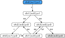
Figure 1: The DTMC semantics of program $\mathsf{Bsp}$.

A reasonable property to be investigated in a reliability analysis would be, e.g., the probability of reaching the deadlock state within 10 rounds. Formally, this probability would be expressed by $\Pr\nolimits_{\mathsf{Prog},\eta}[\Diamond^{<10}\texttt{fail}]$ where $\lambda(\texttt{fail})=(\texttt{cf}=0\wedge x=0)$.

2.2 Live Range Analysis

We present here an adaption of the well-known live range analysis (see, e.g., [2]) to guarded command languages by means of programs. Intuitively, a variable is considered to be live in a variable evaluation of the program if there is an execution where the variable is not written until it is read. As we are interested in reduction methods on a syntactic level, we define an approach based on commands rather than on variable evaluations.

Assume we have given a program $\mathsf{Prog}$ as defined in the last section. By Algorithm 1 we define a function $\mathsf{live}\colon C\rightarrow{\wp}\left(\mathit{Var}\right)$ that returns a set of live variables $\mathsf{live}(c)$ for any command $c\in C$. The function $\mathsf{live}$ is a conservative under-approximation of liveness based on variable evaluations in the sense that there could be variable evaluations $\eta$ where a command $c$ with $v\in\mathsf{live}(c)$ is enabled but $v$ is not live in $\eta$.

input : $\mathsf{Prog}=(\mathit{Var},C,\iota)$

output : $LRA(\mathsf{Prog})\colon C\rightarrow{\wp}\left(\mathit{Var}\right)$

1 $\mathsf{live}:=\mathsf{r}$

2 $U:=C$

3 while $U\neq\varnothing$ do

4       Pick a command $c^{\prime}\in U$

5       $U:=U\setminus\{c^{\prime}\}$

6       forall $c\in\mathsf{pred}(c^{\prime})$ do

7             $I:=\mathsf{live}(c)\cup\big{(}\mathsf{live}(c^{\prime})\setminus\mathsf{w}(c)\big{)}$

8             if $I\neq\mathsf{live}(c)$ then

9                  $\mathsf{live}(c):=I$

10                   $U:=U\cup\{c\}$

11return $\mathsf{live}$

Algorithm 1 Live range analysis ($LRA$)

It is easy to see that Algorithm 1 terminates as in every iteration of the while loop (line 3-10) either at least one new live variable is added to a command or the size of $U$ decreases. Furthermore, Algorithm 1 runs in polynomial time in the size of the input program.

2.3 Graph Coloring

Let us revisit notions for coloring graphs. A graph is a pair $\mathcal{G}=(V,E)$ where $V$ is a finite set of vertices $V$ and $E\subseteq{\wp}\left(V\right)$ is a set of edges where for each $e\in E$ we have $|e|=2$. Given a graph $\mathcal{G}=(V,E)$ and an integer $k\in\mathbb{N}$, a function $f\colon V\rightarrow\{1,\ldots,k\}$ is a $k$-coloring of $\mathcal{G}$ if for all $\{x,y\}\in E$ we have that $f(x)\neq f(y)$. We call $k\in\mathbb{N}$ for which there is a $k$-coloring of $\mathcal{G}$ minimal if there is no $k^{\prime}\in\mathbb{N}$ with $k^{\prime}<k$ where there is a $k^{\prime}$-coloring of $\mathcal{G}$. It is well known that the question whether some $k\in\mathbb{N}$ is minimal is NP-hard [17]. To this end, many heuristic have been proposed to determine nearly minimal graph colorings in reasonable time. In this paper we rely on a greedy heuristics for graph coloring that runs in quadratic time and is due to Welsh and Powell [30], listed in Algorithm 2.

input : $\mathcal{G}=(V,E),V=\{1,\ldots,n\}$

output : $\mathit{WP}(\mathcal{G})\colon V\rightarrow\{1,\ldots,n\}$

1 forall $v\in V$ do

2       $f(v):=0$

3       $d(v):=|\{\{v,v^{\prime}\}\in E:v^{\prime}\in V\}|$

4Let $o\colon\{1,\ldots,n\}\rightarrow V$ such that $d(o(i))\geq d(o(j))$ for all $1{\leq}i{\leq}j{\leq}n$

5 for $c:=1,\ldots,n$ do

6       for $i:=1,\ldots,n$, $f(o(i))=0$ do

7             if $\nexists v.\{o(i),v\}\in E\wedge f(v){=}c$ then

8                  $f(o(i))=c$

9return $f$

Algorithm 2 Welsh-Powell algorithm

3 Reset Value Optimization

The basic idea behind reset value optimization (RVO) [16, 12] is to update variables with a default value as soon as they are not live anymore. This approach has the advantage of being relatively easy to apply on programs even when performed by hand, as after a simple live range analysis it mainly operates locally on commands. Even though it is surprisingly effective.

Algorithm 3 shows the pseudo code of RVO.

input : $\mathsf{Prog}=(\mathit{Var},C,\iota)$; $\rho\in\mathit{Eval}(\mathit{Var})$; $Ex\subseteq\mathit{Var}$

output : $\mathsf{Prog}^{\prime}=(\mathit{Var},C^{\prime},\iota)$

1 $\mathsf{live}:=\mathit{LRA}(\mathsf{Prog})$

2 $C^{\prime}:=\varnothing$

3 forall $c\in C$ do

4       $c^{\prime}=c$

5       forall p:$[$cf:=$\ell,xu]$ in $c$ do

6             $L:=\mathsf{live}(c){\setminus}Ex$

7             forall $s\in C$ with $\mathsf{cf}(s)=\ell$ do

8                   $L:=L{\setminus}\mathsf{live}(s)$

9            forall $x\in L$ do

10                   if there is $x:=e$ in $xu$ then

11                        replace $x:=e$ in $xu$ of $c^{\prime}$ by $x:=\rho(x)$

12                  else

13                        add $x:=\rho(x)$ to $xu$ in $c^{\prime}$

14      $C^{\prime}:=C^{\prime}\cup\{c^{\prime}\}$

15      

16return $(\mathit{Var},C^{\prime},\iota)$

Algorithm 3 RVO

Besides a program $\mathsf{Prog}$ as introduced in Section 2.1, it takes a variable evaluation $\rho$ and a set of variables $Ex$ as input. While $\rho$ specifies the values the variables are reset to, $Ex$ specifies the variables that should be excluded from the optimization, i.e., not reset. Exclusion of variables is required to guarantee bisimilarity [23] w.r.t. atomic-proposition labeling used in properties for analyzing the system. For instance, assume a variable $v$ that is initially $0$ and is set to $1$ when a failure fail occurred. In case $v$ is set to $1$ in the first round of executing $\mathsf{Prog}$, never read again, and no further failure occurs, this variable would eventually be reset to $0$ in a program $\mathsf{Prog}^{\prime}$ that results from RVO on $\mathsf{Prog}$. However, it might be that $\Pr_{\mathsf{Prog},\eta}[\Diamond^{<2}\texttt{fail}]\neq\Pr_{\mathsf{Prog}^{\prime},\eta}[\Diamond^{<2}\texttt{fail}]$ as an execution fulfilling $\Diamond^{<2}\texttt{fail}$ in $\mathsf{Prog}$ might be not present in $\mathsf{Prog}^{\prime}$.

Algorithm 3 iterates through all updates in commands of the program and modifies them depending on a live range analysis (line 5-13): First, the variables that are live in the command’s updates and can serve as reset candidates are stored in a set $L$ (line 6). Then, all live variables in commands that have a control-flow location that is set by the update are disregarded from $L$ (line 7-8), as these are those variables that are further live after the update and hence, the value of these variables matter in future steps. When there are any variables $x$ in $L$ after the removal of future live variables, then these variables can be set to any value without changing the behavior of the program. This is done in line 9 and following. In case there is already an update of the variable $x$ in the list of updates $xu$, then this update is replaced by $x:=\rho(x)$ (line 11), and otherwise $x:=\rho(x)$ is added to the list of updates $xu$ (line 13). It is easy to see that Algorithm 3 terminates and runs in polynomial time as $C$ is finite and $C^{\prime}$ strictly increases every step until $|C^{\prime}|=|C|$.

Theorem 3.1.

Let $\mathsf{Prog}=(\mathit{Var},C,\iota)$ a program, $Ex\subseteq\mathit{Var}$, $\texttt{fail}\in\mathbb{G}(Ex)$, $k\in\mathbb{N}$, and $\mathsf{Prog}^{\prime}$ the program obtained from applying Algorithm 3 on $\mathsf{Prog}$, $Ex$, and some $\rho\in\mathit{Eval}(\mathit{Var})$. Then for every $\eta\in[\![\iota]\!]$

$\Pr\nolimits_{\mathsf{Prog},\eta}[\Diamond^{<k}\texttt{fail}]\enskip=\enskip\Pr\nolimits_{\mathsf{Prog}^{\prime},\eta}[\Diamond^{<k}\texttt{fail}]$.

Example 3.2.

Let us return to our example program introduced in Example 2.1. After applying Algorithm 3 on $\mathsf{Bsp}=(\mathit{Var},C,\iota)$ with $Ex=\varnothing$ and $\rho\in[\![\iota]\!]$ (recall that $\rho$ is uniquely defined as $[\![\iota]\!]$ is a singleton) we obtain a program $\mathsf{Bsp}^{\prime}=(\mathit{Var},C^{\prime},\iota)$ where $C^{\prime}$ comprises commands

$$\begin{array}[]{l}\texttt{cf}=0\wedge x=1\enskip\rightarrow\enskip 1:[\texttt{cf}:=1,x:=0]\\ \texttt{cf}=1\wedge x=0\enskip\rightarrow\\ \enskip 0.5:[\texttt{cf}:=2,{\color[rgb]{1,0,0}x:=1},y:=0]\ +\\ \enskip 0.5:[\texttt{cf}:=3,{\color[rgb]{1,0,0}x:=1},y:=0]\\ \texttt{cf}=2\enskip\rightarrow\enskip 1:[\texttt{cf}:=0,x:=1,{\color[rgb]{1,0,0}y:=1}]\\ \texttt{cf}=3\enskip\rightarrow\\ \enskip 0.3:[\texttt{cf}:=0,x:=0]+0.7:[\texttt{cf}:=1,x:=0]\end{array}$$

In the above commands, we highlighted the changes of the updates in red. According to the program logic, the variable $x$ is not used after the execution of the command that is enabled in control-flow location $\texttt{cf}=1$, since $x$ is not in any guard of commands with control-flow locations $\texttt{cf}=2$ and $\texttt{cf}=3$ where in both cases the value of $x$ is updated. To this end, we can explicitly reset it to the initial value $1$ without changing the program behavior. Likewise, variable $y$ can be reset to $1$ in the command with $\texttt{cf}=2$, as $y$ is not part of the guard of the command with $\texttt{cf}=0$ and is updated in the command of $\texttt{cf}=1$. Figure 2 shows the DTMC semantics of $\mathsf{Bsp}^{\prime}$.

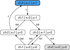
Figure 2: The DTMC semantics of program $\mathsf{Bsp}$ after RVO.

While the DTMC semantics of $\mathsf{Bsp}$ had seven states, the DTMC of Figure 2 has only six states, witnessing the potential of reduction using RVO.

4 Register Allocation Optimization

Ideas from register allocation [2] can be used to reduce the number of variables in a program specification without changing the program’s properties, i.e., strive towards a bisimilar program of reduced size. Within register allocation, the task is to assign variables to a bounded number of resources in terms of memory cells. In contrast to classical register-allocation algorithms, we do not consider a strict bound on the number of memory cells but want to minimize its number, hence not relying on spilling techniques. We adopt Chaitin’s algorithm [7] known for its good minimizations based on coloring interference graphs.

4.1 Interference Graph Coloring

Let $\mathsf{Prog}=(\mathit{Var},C,\iota)$ a program. The interference graph (IG) of $\mathsf{Prog}$ is a graph $\mathcal{G}_{\mathsf{Prog}}=(\mathit{Var},E)$ where $e=\{x,y\}\in E$ iff

• $e\subseteq\mathsf{live}(\mathsf{cf}^{-1}(0))$ or

• there is a $c\in C$ with $e\subseteq\mathsf{live}\big{(}\mathsf{succ}(c)\big{)}$.

Stated in words, two variables in the IG are connected in case they are not simultaneously live in either the initial commands or while executing a command. This intuitively means that one cannot use the same memory cell to store both variables, i.e., cannot merge them. The construction of IG is doable in time polynomial in the size of $\mathsf{Prog}$.

To obtain sets of variables that can be merged, the idea is to determine a coloring of the IG and merge $x,y\in\mathit{Var}$ in case $x$ and $y$ have the same color. For obtaining a graph coloring with a nearly minimal number of colors, we rely on the Welsh-Powell heuristics provided in Algorithm 2.

4.2 Variable Merging

Algorithm 4 shows our register allocation optimization based on a given coloring of the program’s IG. As within RVO presented in Algorithm 3, this algorithm takes as input also a set of variables $Ex\subseteq\mathit{Var}$ to be excluded from optimization to ensure bisimilarity w.r.t. atomic propositions used in property specifications.

input : $\mathsf{Prog}=(\mathit{Var},C,\iota)$; $Ex\subseteq\mathit{Var}$

output : $\mathsf{Prog}^{\prime}=(\mathit{Var}^{\prime},C^{\prime},\iota^{\prime})$

1 $\mathsf{wp}:=\mathit{WP}(\mathcal{G}_{\mathsf{Prog}})$

2 $\mathit{Var}^{\prime}=Ex\cup\{v_{i}:\exists v,i.\mathsf{wp}(v)=i\}$

3 $C^{\prime}:=C$, $\iota^{\prime}:=\iota$

4 forall $v\in\mathit{Var}{\setminus}Ex$ do

5       replace $v$ in $C^{\prime}$ and $\iota^{\prime}$ by $v_{\mathsf{wp}(v)}$

6      

7return $(\mathit{Var}^{\prime},C^{\prime},\iota^{\prime})$

Algorithm 4 RAO

In line 1, we apply Algorithm 2 on the IG of the input program $\mathsf{Prog}$. Line 2 specifies the new set of variables $\mathit{Var}^{\prime}$ as the excluded variables $Ex$ from $\mathit{Var}$ (to guarantee correctness of analysis results w.r.t. properties over $\mathbb{G}(Ex)$) and merged variables. The rest of the algorithm simply replaces any occurrence of variables not excluded from optimization by their merged counterparts. Algorithm 4 runs in polynomial time as its complexity is dominated by the live range analysis (see Algorithm 1), the construction of IG, and the Welsh-Powell algorithm (see Algorithm 2).

Theorem 4.1.

Let $\mathsf{Prog}=(\mathit{Var},C,\iota)$ a program, $Ex\subseteq\mathit{Var}$, $\texttt{fail}\in\mathbb{G}(Ex)$, $k\in\mathbb{N}$, and $\mathsf{Prog}^{\prime}$ the program obtained from applying Algorithm 4 on $\mathsf{Prog}$ and $Ex$. Then for every $\eta\in[\![\iota]\!]$

$\Pr\nolimits_{\mathsf{Prog},\eta}[\Diamond^{<k}\texttt{fail}]\enskip=\enskip\Pr\nolimits_{\mathsf{Prog}^{\prime},\eta}[\Diamond^{<k}\texttt{fail}]$.

Example 4.2.

Let us again return to our example program introduced in Example 2.1. After applying Algorithm 4 on $\mathsf{Bsp}=(\mathit{Var},C,\iota)$ with $Ex=\varnothing$ we obtain a program $\mathsf{Bsp}^{\prime}=(\mathit{Var}^{\prime},C^{\prime},\iota^{\prime})$ where $\mathit{Var}=\{xy\}$, $\iota^{\prime}=(xy=1)$, and $C^{\prime}$ comprises the commands

$$\begin{array}[]{l}\texttt{cf}=0\wedge{\color[rgb]{1,0,0}xy=1}\enskip\rightarrow\enskip 1:[\texttt{cf}:=1,{\color[rgb]{1,0,0}xy:=0}]\\ \texttt{cf}=1\wedge{\color[rgb]{1,0,0}xy=0}\enskip\rightarrow\\ \enskip 0.5:[\texttt{cf}:=2,{\color[rgb]{1,0,0}xy:=0}]\ +\\ \enskip 0.5:[\texttt{cf}:=3,{\color[rgb]{1,0,0}xy:=0}]\\ \texttt{cf}=2\enskip\rightarrow\enskip 1:[\texttt{cf}:=0,{\color[rgb]{1,0,0}xy:=1}]\\ \texttt{cf}=3\enskip\rightarrow\enskip 0.3:[\texttt{cf}:=0,{\color[rgb]{1,0,0}xy:=0}]\ +\\ \hskip 55.8001pt0.7:[\texttt{cf}:=1,{\color[rgb]{1,0,0}xy:=0}]\end{array}$$

Again, we highlighted the changes of the commands compared to $\mathsf{Bsp}$ in red. Already in Example 3.2, we saw that $x$ and $y$ do not interfere in resets and the use of them in guards. It is hence not too surprising that we can merge them into one variable $v_{1}=xy$ according to Algorithm 4. Figure 3 shows the DTMC semantics of $\mathsf{Bsp}^{\prime}$.

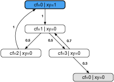
Figure 3: The DTMC semantics of program $\mathsf{Bsp}$ after RAO.

The arising DTMC has even one state less than the DTMC obtained after application of RVO (see Figure 2), showing the potential of even further reductions on programs through RAO.

5 Implementation and Evaluation

We implemented both reduction methods as Python programs that accept a model in the input language of the prominent probabilistic model checker Prism [22], together with a variable used as control-flow variable, and a set of variables to be excluded from the optimization.

Statistics of the reliability analysis experiments reduction model size reduction times [s] speedup method states nodes states nodes IVR build analysis $\sum$ no 4.87$\cdot 10^{13}$ 301 733 - - 1895.6 708.6 1 226.2 3 830.4 - RVO 1.02$\cdot 10^{11}$ 233 020 477.3 1.3 270.4 275.5 915.0 1 190.4 3.2 RAO 4.30$\cdot 10^{10}$ 121 426 1 133.1 2.5 125.8 82.3 296.8 379.1 10.1

The VCL model.

We applied our reduction methods on a simplified version of the aircraft model borrowed from the Simulink example set [1] that itself is based on a long-haul passenger aircraft flying at cruising altitude and speed, adjusting the fuel flow rate to control the aircraft velocity. Following the approach of [12], we generated a model family that includes options to protect Simulink blocks via redundancy mechanisms to increase fault tolerance of the velocity control loop (VCL). Specifically, we considered 13 Simulink blocks protectable with
comparison: The block is duplicated and both outputs are compared. In case their output differs a dedicated failure state is reached. Otherwise, the output is the one of both blocks.
voting: Following the principle of triple modular redundancy principle, the block is triplicated and the output is based on a majority decision.
The arising model comprises $3^{13}=1\,594\,323$ different variants of the VCL. Using OpenErrorPro [25], we automatically generated a Prism model on which we applied the reduction methods RVO and RAO presented in this paper. Here, we modeled errors that could appear during the execution of a Simulink block function, e.g., caused by a bit-flip in a CPU. The occurrence of such an error is determined stochastically with the probabilities that depend on the commands in the Simulink block functions. Even after the reductions, the model could not immediately be constructed by Prism’s symbolic engine. This was as expected, since also the VCL model considered in [12] could not be constructed ad-hoc even given the model presented there considered only eight block to be protectable. We hence applied a method called iterative variable reordering (IVR) [13] to enable model construction. It is well known that symbolic methods based on BDDs [24] as used in Prism’s symbolic engine are sensitive to the so-called variable order. The main idea behind IVR is to iteratively enlarge the system family and perform variable reorderings at each step to eventually obtain a suitable variable order for the whole system family. Specifically, we applied the automated IVR method presented in [13], following a $\rho$-maximal selection heuristics with step size four and using the variable reordering implementation of [19]. Table 5 shows statistics of the arising model sizes and construction timings. While the number of nodes used to represent the model symbolically is not significantly reduced, the explicit state-space representation could be reduced drastically in 2-3 orders of magnitude.

Reliability analysis.

We performed a reliability analysis on the constructed VCL model family to determine the probability of the system to fail within two rounds of execution. All experiments were carried out on a Linux server system (2 $\times$ Intel Xeon E5-2680 (Octa Core, Sandy Bridge) running at 2.70 GHz with 384 GB of RAM; Turbo Boost and Hyper Threading disabled; Debian GNU/Linux 9.1) with a memory bound of 30 GB of RAM, running the symbolic MTBDD engine of the Prism version presented in [19]. Specifically, we computed $\Pr_{\mathsf{VCL},\pi}(\Diamond^{<2}\texttt{fail})$ for every protection combination $\pi$ using a family-based all-in-one analysis [11]. The results range from $0.435$ probability to fail with no protection mechanism and $0.019$ with all 13 blocks protected. Table 5 shows the timing statistics of the analysis where an overall speedup of an order of magnitude turns out to be possible with our reduction methods.

Comparison to [12].

In [12] we proposed to use family-based methods for the analysis of redundancy systems modeled in Simulink, issuing a VCL model family with eight blocks eligible for protection and four protection mechanisms. This led to a family size of $4^{8}=65\,536$. There, we applied preliminary versions of IVR and RVO in a handcrafted fashion, not exploiting their full potential, e.g., leaving out variables that could possibly reset. In this paper, automated techniques enabled us to perform a reliability analysis on a much bigger instance with $3^{13}$ family members.

6 Discussion and Further Work

To the best of our knowledge, we were the first presenting fully automated reduction methods for probabilistic programs that purely operate on a syntactic level. The presented approaches are not only applicable to Prism programs with a dedicated formalism of control flow, but also to arbitrary Prism programs. However, such optimizations might be not as effective since LRA heavily relies on the concept of control flows. In this sense, although we applied our methods on DTMC models only, they can be also useful for other models expressed in Prism’s input language, e.g., Markov decision processes. Further, our methods yield bisimilar models for arbitrary temporal logical formulas expressed over the set of excluded variables. Since we strived towards reliability analysis, we presented the approach in a simpler form of reward-bounded reachability properties. Although RVO uses Chaitin’s algorithm, we could use our methods also with the linear scan algorithm (LSA) [26], e.g., to enable fast reduction methods for runtime verification [15]. When bounded model checking [6] is used as analysis method, an idea is to adapt LRA such that it considers live ranges up to the desired model-checking bound. We showed that our methods are effective especially when explicit model representations are used. As explicit model-checking methods are well known to be faster than symbolic methods when applied on relatively small models, we expect also such models to benefit from our reduction methods presented.

Acknowledgments.

This work is supported by the DFG through the Collaborative Research Center TRR 248 (see https://perspicuous-computing.science, project ID 389792660), the Cluster of Excellence EXC 2050/1 (CeTI, project ID 390696704, as part of Germany’s Excellence Strategy), the Research Training Groups QuantLA (GRK 1763) and RoSI (GRK 1907), projects JA-1559/5-1, BA-1679/11-1, BA-1679/12-1, and the 5G Lab Germany.

References

- [1] Verify model using simulink control design and simulink verification blocks (accessed 19/02/2019). https://mathworks.com/help/slcontrol/ug/model-verification-using-simulink-control-design-and-simulink-verification-blocks-.html.
- Aho and Ullman [1977] A. V. Aho and J. D. Ullman. Principles of compiler design. Series in computer science and information processing. Addison-Wesley, Reading, MA, 1977.
- Baier and Katoen [2008] C. Baier and J.-P. Katoen. Principles of Model Checking. MIT Press, 2008.
- Baier et al. [2006] C. Baier, P. D’Argenio, and M. Groesser. Partial order reduction for probabilistic branching time. In Proc. of the 3rd Workshop on Quantitative Aspects of Programming Languages, volume 153, pages 97 – 116, 2006.
- Baier et al. [2014] C. Baier, M. Daum, C. Dubslaff, J. Klein, and S. Klüppelholz. Energy-utility quantiles. In 6th NASA Formal Methods Symposium (NFM), volume 8430 of Lecture Notes in Computer Science, pages 285–299, 2014.
- Biere et al. [2003] A. Biere, A. Cimatti, E. M. Clarke, O. Strichman, Y. Zhu, et al. Bounded model checking. Advances in computers, 58(11):117–148, 2003.
- Chaitin [2004] G. Chaitin. Register allocation and spilling via graph coloring. SIGPLAN Not., 39(4):66–74, 2004.
- Chrszon et al. [2018] P. Chrszon, C. Dubslaff, S. Klüppelholz, and C. Baier. Profeat: feature-oriented engineering for family-based probabilistic model checking. Formal Aspects of Computing, 30(1):45–75, 2018.
- Dehnert et al. [2017] C. Dehnert, S. Junges, J. Katoen, and M. Volk. A Storm is coming: A modern probabilistic model checker. In 29th Int. Conf. on Computer Aided Verification (CAV), volume 10427 of LNCS, pages 592–600. Springer, 2017.
- Dijkstra [1975] E. W. Dijkstra. Guarded commands, nondeterminacy and formal derivation of programs. Commun. ACM, 18(8):453–457, 1975.
- Dubslaff et al. [2015] C. Dubslaff, C. Baier, and S. Klüppelholz. Probabilistic model checking for feature-oriented systems. Transactions on Aspect-Oriented Software Development, 12:180–220, 2015.
- Dubslaff et al. [2019] C. Dubslaff, K. Ding, A. Morozov, C. Baier, and K. Janschek. Breaking the limits of redundancy systems analysis. In Proceedings of the 29th European Safety and Reliability Conference, pages 2317–2325, 2019.
- Dubslaff et al. [2020] C. Dubslaff, A. Morozov, C. Baier, and K. Janschek. Iterative variable reordering: Taming huge system families. In Proceedings of the 4th Workshop on Models for Formal Analysis of Real Systems, EPTCS, pages 82–94, 2020.
- Forejt et al. [2011] V. Forejt, M. Z. Kwiatkowska, G. Norman, and D. Parker. Automated verification techniques for probabilistic systems. In 11th International School on Formal Methods for the Design of Computer, Communication and Software Systems (SFM), volume 6659 of LNCS, pages 53–113, 2011.
- Forejt et al. [2013] V. Forejt, M. Z. Kwiatkowska, D. Parker, H. Qu, and M. Ujma. Incremental runtime verification of probabilistic systems. In Proc. of the 3rd International Conference on Runtime Verification (RV), volume 7687 of LNCS, pages 314–319. Springer, 2013.
- Garavel and Serwe [2006] H. Garavel and W. Serwe. State space reduction for process algebra specifications. Theoretical Computer Science, 351(2):131 – 145, 2006. 10.1016/j.tcs.2005.09.064. Algebraic Methodology and Software Technology.
- Garey and Johnson [1979] M. R. Garey and D. S. Johnson. Computers and Intractability: A Guide to the Theory of NP-Completeness. W. H. Freeman & Company, 1979. ISBN 0-7167-1044-7.
- Katoen [2016] J. Katoen. The probabilistic model checking landscape. In Proceedings of the 31st Annual ACM/IEEE Symposium on Logic in Computer Science, LICS ’16, New York, NY, USA, July 5-8, 2016, pages 31–45, 2016.
- Klein et al. [2018] J. Klein, C. Baier, P. Chrszon, M. Daum, C. Dubslaff, S. Klüppelholz, S. Märcker, and D. Müller. Advances in probabilistic model checking with PRISM: variable reordering, quantiles and weak deterministic Büchi automata. Intern. Journal on Software Tools for Technology Transfer, 20(2):179–194, 2018.
- Kulkarni [1995] V. G. Kulkarni. Modeling and Analysis of Stochastic Systems. Chapman & Hall, 1995.
- Kwiatkowska et al. [2006] M. Kwiatkowska, G. Norman, and D. Parker. Symmetry reduction for probabilistic model checking. In Proc. of the 18th International Conference on Computer Aided Verification (CAV ’06), volume 4114 of LNCS, pages 234–248. Springer, 2006.
- Kwiatkowska et al. [2011] M. Kwiatkowska, G. Norman, and D. Parker. PRISM 4.0: Verification of probabilistic real-time systems. In G. Gopalakrishnan and S. Qadeer, editors, Proc. 23rd International Conference on Computer Aided Verification (CAV’11), volume 6806 of LNCS, pages 585–591. Springer, 2011.
- Larsen and Skou [1991] K. G. Larsen and A. Skou. Bisimulation through probabilistic testing. Information and Computation, 94(1):1 – 28, 1991.
- McMillan [1993] K. L. McMillan. Symbolic Model Checking. Kluwer, 1993.
- Morozov et al. [2019] A. Morozov, K. Ding, M. Steurer, and K. Janschek. Openerrorpro: A new tool for stochastic model-based reliability and resilience analysis. In 2019 IEEE 30th International Symposium on Software Reliability Engineering (ISSRE), pages 303–312. IEEE, 2019.
- Poletto and Sarkar [1999] M. Poletto and V. Sarkar. Linear scan register allocation. ACM Transactions on Programming Languages and Systems (TOPLAS), 21(5):895–913, 1999.
- Puterman [1994] M. Puterman. Markov Decision Processes. Wiley, 1994.
- The MathWorks Inc. [2018] The MathWorks Inc. MATLAB and Statistics Toolbox Release 2018b. Natick, Massachusetts, United States, 2018.
- Volk et al. [2018] M. Volk, S. Junges, and J. Katoen. Fast dynamic fault tree analysis by model checking techniques. IEEE Trans. Industrial Informatics, 14(1):370–379, 2018.
- Welsh and Powell [1967] D. J. A. Welsh and M. B. Powell. An upper bound for the chromatic number of a graph and its application to timetabling problems. Comput. J., 10:85–86, 1967.