Star Formation Occurs in Dense Gas, but What Does “Dense” Mean?

Abstract

We report results of a project to map HCN and HCO⁺  $J=1\rightarrow 0$ emission toward a sample of molecular clouds in the inner Galaxy, all containing dense clumps that are actively engaged in star formation. We compare these two molecular line tracers with millimeter continuum emission and extinction, as inferred from ¹³CO, as tracers of dense gas in molecular clouds. The fraction of the line luminosity from each tracer that comes from the dense gas, as measured by $\mbox{$A_{\rm V}$}>8$ mag, varies substantially from cloud to cloud. In all cases, a substantial fraction (in most cases, the majority) of the total luminosity arises in gas below the $\mbox{$A_{\rm V}$}>8$ mag threshold and outside the region of strong mm continuum emission. Measurements of $L({\rm HCN})$ toward other galaxies will likely be dominated by such gas at lower surface density. Substantial, even dominant, contributions to the total line luminosity can arise in gas with densities typical of the cloud as a whole ($n\sim 100$ cm^-3). Defining the dense clump from the HCN or HCO⁺ emission itself, similarly to previous studies, leads to a wide range of clump properties, with some being considerably larger and less dense than in previous studies. HCN and HCO⁺ have similar ability to trace dense gas for the clouds in this sample. For the two clouds with low virial parameters, the ¹³CO is definitely a worse tracer of the dense gas, but for the other four, it is equally good (or bad) at tracing dense gas.

1 Introduction

In pioneering work, Gao & Solomon (2004) showed that the far-infrared luminosities in starburst galaxies followed a very tight, linear correlation with the luminosities of HCN line emission. Wu et al. (2005) showed that this relationship extended to massive, dense clumps in the Milky Way, arguing that the fundamental unit of massive, clustered star formation is such a massive, dense clump. Subsequent studies have defined a “threshold” surface density of $\mbox{$A_{\rm V}$}>8$ mag (about 120 M_⊙ pc^-2) in nearby clouds (Heiderman et al. 2010; Lada et al. 2010, 2012) above which the vast majority of dense cores and YSOs are found. Evans et al. (2014) compared various models of star formation to observations of the nearby clouds and found that the mass of dense gas was the best predictor of the star formation rate. Most recently, Vutisalchavakul et al. (2016) showed that a similar result applied to more distant and massive clouds in the Galactic Plane, using millimeter continuum emission from the BGPS survey (Ginsburg et al. 2013) to measure the mass of dense gas. Vutisalchavakul et al. (2016) found a substantial dispersion in the star formation rate per mass of dense gas (0.50 dex), but the logarithmic averages of the star formation rate per mass of dense gas were in general agreement for nearby clouds, inner Galaxy clouds, and extragalactic clouds. The dispersion among the averages for all those was only 0.19 dex (figure 11 of Vutisalchavakul et al. 2016), considerably lower than that for total molecular gas probed by CO or ¹³CO, 0.42 dex (figure 12 of Vutisalchavakul et al. 2016). The star formation rate per unit mass of dense gas is thus remarkably constant over a huge range of scales and conditions. A recent detailed study of HCN emission toward other galaxies (Jiménez-Donaire et al. 2019) also found a small dispersion (0.22 dex) in the star formation rate per mass of dense gas. After accounting for galaxy-to-galaxy variations, the intra-galaxy dispersion was only 0.12 dex. A smaller dispersion for measurements over a whole galaxy is expected if the dispersion among clouds within a galaxy is due to variations in evolutionary state of the molecular cloud (e.g., Kruijssen et al. 2018).

While the tight connection between dense parts of molecular clouds and star formation is clear, we must better define what we mean by “dense.” The most direct measure exists for the nearby clouds, where surface density can be determined by extinction maps of background stars. For the Galactic Plane clouds, continuum emission by dust or line emission by HCN was used. For other galaxies, HCN emission has been the only tracer of dense gas in general use, although HCO⁺ emission has also been explored (Barnes et al. 2011; Privon et al. 2015; Jiménez-Donaire et al. 2019). The extinction maps are strictly sensitive to surface density, while the dust continuum emission is sensitive also to temperature, and the molecular line emission, in addition to surface density and temperature, is sensitive to volume density and abundances. Temperature and molecular abundances can depend on the radiation environment (Shimajiri et al. 2017; Pety et al. 2017). A detailed comparison of these various tracers of “dense” gas can clarify the situation. In this paper, we will compare maps of HCN, HCO⁺, and ¹³CO $J=1\rightarrow 0$ emission to the regions selected as dense by extinction or millimeter-wave continuum emission in a sample of Galactic Plane clouds. We refer to all the molecular lines as “line tracers” and the HCN and HCO⁺ lines as “dense line tracers” for convenience, while noting that our purpose is to test the proposition that they trace gas of the density relevant to star formation.

Specifically, we can learn what fraction of the luminosity from the line tracers arises from low-level, extended emission from less dense gas. Stephens et al. (2016) have argued that most of the Galaxy’s luminosity of HCN arises from distributed, very sub-thermal, emission rather than from dense gas. Since observations of other galaxies would integrate large areas of low-level emission, their HCN luminosity could be dominated by the same gas that is probed by CO, complicating the connection found by Wu et al. (2005) between dense clumps in the Milky Way and other galaxies. Pioneering work by Helfer & Blitz (1997) showed that HCN emission is very weak compared to CO ($I_{\rm HCN}/I_{\rm CO}=0.014\pm 0.020$) averaged over random observations of the Galactic Plane. They further showed that maps of HCN $J=1\rightarrow 0$ in nearby large molecular clouds were tiny in comparison to the CO maps. This work argues against the idea of Stephens et al. (2016) but improved instrumentation now allows a much stronger test. Recent work has shown that HCN emission can indeed arise from more extended regions (Pety et al. 2017; Kauffmann et al. 2017; Shimajiri et al. 2017), but those studies were all toward clouds in the solar neighborhood (out to the distance of the Orion clouds).

Maps of the full extent of ¹³CO emission in inner Galaxy clouds allow us to test directly the contribution of more diffuse molcular gas to the HCN luminosity in a very different environment. The simultaneous observations of HCO⁺ provide a direct comparison of these two tracers. One might predict that HCO⁺ $J=1\rightarrow 0$ traces more wide-spread gas of lower mean density than does HCN $J=1\rightarrow 0$ because the critical density for HCO⁺ $J=1\rightarrow 0$ at $\mbox{$T_{\rm K}$}=20$ K ($n_{\rm cr}\approx 4.5\mbox{${}\times 10^{4}$}$ cm^-3) is nearly an order of magnitude less than that for HCN $J=1\rightarrow 0$ ($n_{\rm cr}\approx 3.0\mbox{${}\times 10^{5}$}$ cm^-3) (Evans 1999; Shirley 2015). Comparison of these two tracers in a well-defined sample with star formation rates will be useful for evaluating relations seen in extragalactic studies of dense gas relations. Studies of HCN and HCO⁺ have found some evidence of environmental effects in other galaxies, such as the presence of an AGN (see, e.g., Privon et al. 2015 for a discussion of this issue.) It is important first to understand the relation between these two tracers in more controlled environments. We also evaluate whether ¹³CO $J=1\rightarrow 0$ can trace the relevant gas for star formation; while it has a much lower critical density ($n_{\rm cr}\approx 4.8\mbox{${}\times 10^{2}$}$ cm^-3), it is easier to observe.

With spectrally resolved maps, we can also assess the balance between gravity and turbulence, most simplistically captured in the virial parameter. One attractive explanation for the low star formation efficiency in molecular clouds is that most clouds are not gravitationally bound, but only relatively dense regions within them are bound (Dobbs et al. 2011; Barnes et al. 2016). By calculating the virial ratio for the structures traced by the different species, we may be able to shed light on this issue.

2 Sample

The target clouds (listed in Table 1) comprise a subset of the Vutisalchavakul et al. (2016) sample, chosen to sample a range of conditions and environments, as well as for suitable size (8 to 35 pc) and lack of confusion. The sample has maps of CO and ¹³CO  and millimeter-wave continuum emission from the Bolocam Galactic Plane Survey (BGPS), (Aguirre et al. 2011; Ginsburg et al. 2013), and two measures of the star formation rate, radio continuum and mid-infrared emission

The typical angular extent of BGPS sources is a few arcmin, so we selected clouds with ¹³CO extents of 10′ to 20′ to fully sample the “diffuse” gas. The boundaries of the ¹³CO emission (column 9 of Table 1) were set in order to separate the cloud from the background; they were substantial and varied from cloud to cloud. These thresholds are 5 to 12 times the RMS noise, so the clouds undoubtedly are larger and more massive, but confusion in the inner Galaxy limits the region that can be isolated. We favored clouds with at least one BGPS source with a size of at least 3′ so that we can clearly compare the morphology of the HCN/HCO⁺ emission and the dust emission. We also favored clouds with larger and stronger BGPS sources. We identified 6 clouds in the sample of Vutisalchavakul et al. (2016) that meet these criteria. The sample spans a good range of cloud mass (2.4${}\times 10^{4}$ M_⊙ to 3.3${}\times 10^{5}$ M_⊙), dense gas mass (700 to 1.3${}\times 10^{4}$ M_⊙), and star formation rate (23 to 275 M_⊙ Myr^-1). While the clouds range in distance from us (3.5 to 10.4 kpc), all lie between 5.1 and 6.4 kpc from the Galactic center, in the molecular ring.

The distances used by Vutisalchavakul et al. (2016) were mostly taken from Anderson et al. (2014), who used a variety of sources of information on the velocity and methods for kinematic distance ambiguity resolution (KDAR). We now have velocities of the dense gas traced best by H¹³CO⁺ or HCO⁺ (see later section) and there are newer distance estimators. We recalculated the distances using the tool described in Wenger et al. (2018), which provides a distance pdf and two-sided uncertainties. While we use the two-sided uncertainties, they are in general fairly symmetric. We use the same choice of near, far, or tangent point distances as Anderson et al. (2014) (noted by N, F, or T in the KDAR column of Table 1). In particular, G037.677$+$00.155 was placed at the tangent point because its velocity was within 10 km s^-1 of the velocity at the tangent point. We have scaled the sizes, cloud masses, dense gas masses, and star formation rates to the new distances and propagated the uncertainties in the distance to uncertainties in other quantities. The distance uncertainties typically dominate if they enter the calculation of a quantity. We use the star formation rates from the mid-infrared emission. The results are in Table 1. As discussed in detail in the Appendix, we use the kinematic distance to G034.158$+$00.147 rather than the closer distance from maser parallax. The latter is quite uncertain and would require an unreasonably large (40 km s^-1) peculiar motion.

Table 1: Sample of Clouds

Source	$d$	KDAR	Size	Log $M_{\rm cloud}$	Log $M_{\rm dense}$	Log SFR	Map Size	13CO Lim	Note
	(kpc)		(pc)	(M⊙)	(M⊙)	(M⊙/Myr)	($\arcmin\times\arcmin$)	(K)
G034.158$+$00.147	$3.48^{+0.43}_{-0.32}$	N	$22.68^{+2.80}_{-2.09}$	$4.75^{+0.17}_{-0.25}$	$4.13^{+0.10}_{-0.09}$	$2.44^{+0.10}_{-0.10}$	$30\times 30$	2.2
G034.997$+$00.330	$10.43^{+0.38}_{-0.41}$	F	$35.41^{+1.29}_{-1.39}$	$5.52^{+0.15}_{-0.23}$	$4.08^{+0.15}_{-0.23}$	$1.85^{+0.05}_{-0.06}$	$10\times 20$	2.6	1
G036.459$-$00.183	$8.68^{+0.56}_{-0.60}$	F	$17.21^{+1.11}_{-1.19}$	$4.96^{+0.15}_{-0.24}$	$3.49^{+0.15}_{-0.23}$	$1.36^{+0.07}_{-0.08}$	$14\times 22$	2.2	1
G037.677$+$00.155	$6.60^{+0.13}_{-0.14}$	T	$27.15^{+0.53}_{-0.58}$	$5.45^{+0.15}_{-0.23}$	$3.02^{+0.16}_{-0.25}$	$2.09^{+0.04}_{-0.05}$	$10\times 26$	1.9
G045.825$-$00.291	$8.31^{+0.46}_{-0.62}$	F	$25.69^{+1.42}_{-1.92}$	$5.41^{+0.15}_{-0.24}$	$3.91^{+0.15}_{-0.24}$	$1.87^{+0.06}_{-0.09}$	$30\times 30$	1.6
G046.495$-$00.241	$3.71^{+0.68}_{-0.60}$	N	$8.27^{+1.52}_{-1.34}$	$4.38^{+0.19}_{-0.32}$	$2.85^{+0.19}_{-0.32}$	$1.81^{+0.14}_{-0.18}$	$20\times 10$	1.6

Notes: 1. Mapped in equatorial Coordinates

3 Observations

We mapped the six clouds in the HCN (1$-$0) (88.631847 GHz) (DeLucia & Gordy 1969) and HCO⁺ (1$-$0) (89.188526 GHz) (Sastry et al. 1981) lines simultaneously using the SEQUOIA array with 16 pixels in a 4$\times$4 array at the 14-m telescope of the Taeduk Radio Astronomy Observatory (TRAO) (Roh & Jung 1999; Jeong et al. 2019). The observations were conducted by the On-The-Fly (OTF) technique in the absolute position switching mode with OFF positions checked to be free from appreciable emission. The mapped areas were different for the individual clouds (Table 1). G034.997+00.330 and G036.459$-$00.183 were mapped in equatorial coordinates occasionally between February and May in 2017, while the others were mapped in Galactic coordinates between January and April in 2018. The backend was a 2G FFT spectrometer that can accept 32 signal streams at the same time. Thus it is possible to observe two transitions simultaneously between 85 and 100 GHz or 100 and 115 GHz. The backend bandwidth is 62.5 MHz with 4096 channels, yielding a velocity resolution of 0.05 km s^-1. The observed line temperature was calibrated on the $T_{\rm A}^{*}$ scale by the standard chopper wheel method. We checked the telescope pointing and focus every 3 hours by observing strong SiO maser sources at 86 GHz. The pointing accuracy was better than 10^′′. The system temperatures depended on the weather condition and source elevation. They were usually around 200 K during the observing runs. The RMS noise levels of the observed spectra were typically about 0.1 K after smoothing to 0.2 km s^-1 resolution. We smoothed the data with the boxcar function to a velocity resolution of about 0.2 km s^-1 when fitting line profiles, but some analysis of the data cubes was done with the original resolution. To assess optical depth effects, we observed the innermost footprint in the lines of H¹³CN and H¹³CO⁺

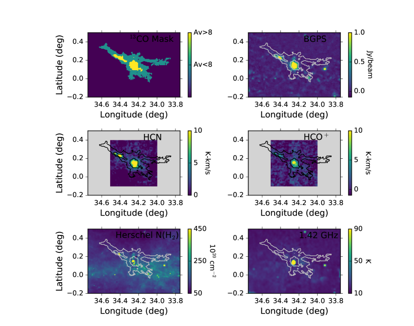
Figure 1: This figure is for the cloud G034.158$+$00.147. Except for the upper left panel, the GRS ¹³CO contours are shown in black or white, depending on the panel, along with images of other tracers or masks. Upper left is the mask for column density $\mbox{$A_{\rm V}$}\geq 8$ mag and the outermost contour of ¹³CO emission; upper right is the BGPS millimeter-wave continuum emission in color with the ¹³CO contour in white; middle left is the HCN integrated intensity in color with the ¹³CO contour in black; middle right is the HCO⁺ integrated intensity in color with the ¹³CO contour in black; lower left is the gas column density determined from Herschel in color with the ¹³CO contour in white; lower right is the 1.42 GHz radio continuum emission in color with the ¹³CO contour in white; The size of the box in the middle panels shows the region mapped in HCN and HCO⁺. The ¹³CO is in units of K km s^-1($T_{\rm mb}$) scaled 0 to 50 K km s^-1; Color bars indicate the range and scaling of the other tracers.

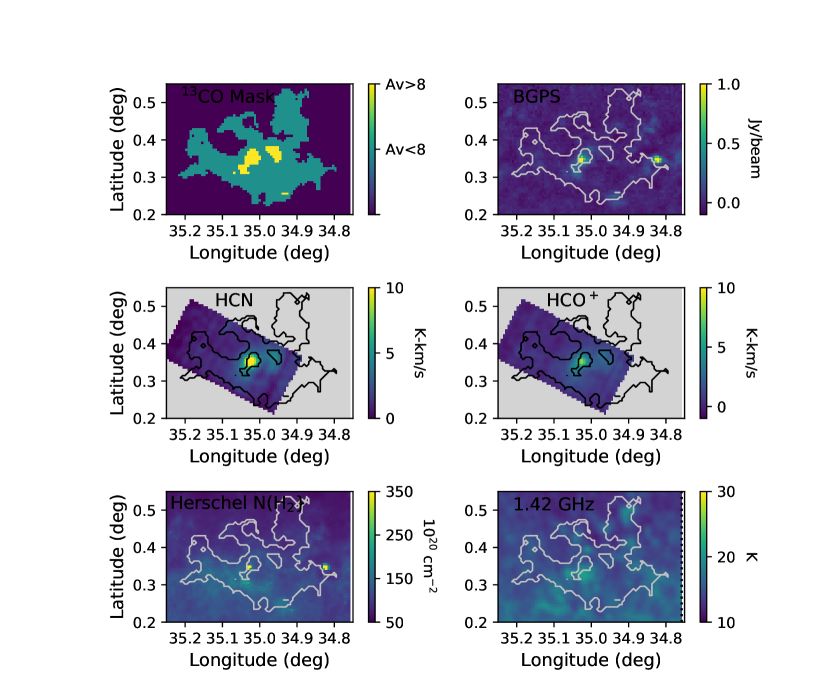
Figure 2: This figure is for the cloud G034.997$+$00.330. Except for the upper left panel, the GRS ¹³CO contours are shown in black or white, depending on the panel, along with images of other tracers or masks. Upper left is the mask for column density $\mbox{$A_{\rm V}$}\geq 8$ mag and the outermost contour of ¹³CO emission; upper right is the BGPS millimeter-wave continuum emission in color with the ¹³CO contour in white; middle left is the HCN integrated intensity in color with the ¹³CO contour in black; middle right is the HCO⁺ integrated intensity in color with the ¹³CO contour in black; lower left is the gas column density determined from Herschel in color with the ¹³CO contour in white; lower right is the 1.42 GHz radio continuum emission in color with the ¹³CO contour in white; The size of the box in the middle panels shows the region mapped in HCN and HCO⁺. The ¹³CO is in units of K km s^-1($T_{\rm mb}$) scaled 0 to 50 K km s^-1; Color bars indicate the range and scaling of the other tracers.

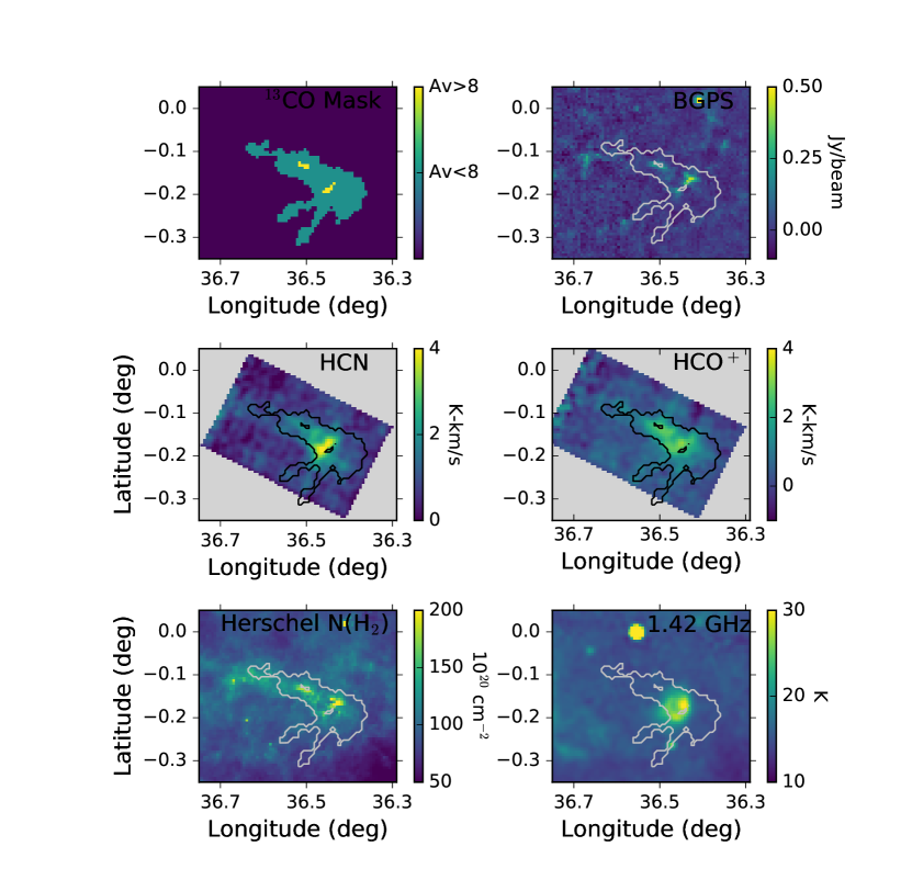
Figure 3: This figure is for the cloud G036.459$-$00.183. Except for the upper left panel, the GRS ¹³CO contours are shown in black or white, depending on the panel, along with images of other tracers or masks. Upper left is the mask for column density $\mbox{$A_{\rm V}$}\geq 8$ mag and the outermost contour of ¹³CO emission; upper right is the BGPS millimeter-wave continuum emission in color with the ¹³CO contour in white; middle left is the HCN integrated intensity in color with the ¹³CO contour in black; middle right is the HCO⁺ integrated intensity in color with the ¹³CO contour in black; lower left is the gas column density determined from Herschel in color with the ¹³CO contour in white; lower right is the 1.42 GHz radio continuum emission in color with the ¹³CO contour in white; The size of the box in the middle panels shows the region mapped in HCN and HCO⁺. The ¹³CO is in units of K km s^-1($T_{\rm mb}$) scaled 0 to 50 K km s^-1; Color bars indicate the range and scaling of the other tracers.

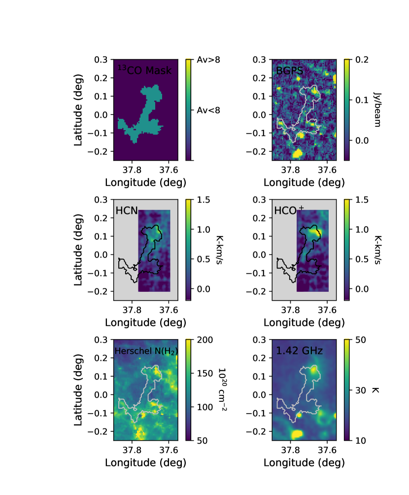
Figure 4: This figure is for the cloud G037.677$+$00.155. Except for the upper left panel, the GRS ¹³CO contours are shown in black or white, depending on the panel, along with images of other tracers or masks. Upper left is the mask for column density $\mbox{$A_{\rm V}$}\geq 8$ mag and the outermost contour of ¹³CO emission; upper right is the BGPS millimeter-wave continuum emission in color with the ¹³CO contour in white; middle left is the HCN integrated intensity in color with the ¹³CO contour in black; middle right is the HCO⁺ integrated intensity in color with the ¹³CO contour in black; lower left is the gas column density determined from Herschel in color with the ¹³CO contour in white; lower right is the 1.42 GHz radio continuum emission in color with the ¹³CO contour in white; The size of the box in the middle panels shows the region mapped in HCN and HCO⁺. The ¹³CO is in units of K km s^-1($T_{\rm mb}$) scaled 0 to 50 K km s^-1; Color bars indicate the range and scaling of the other tracers.

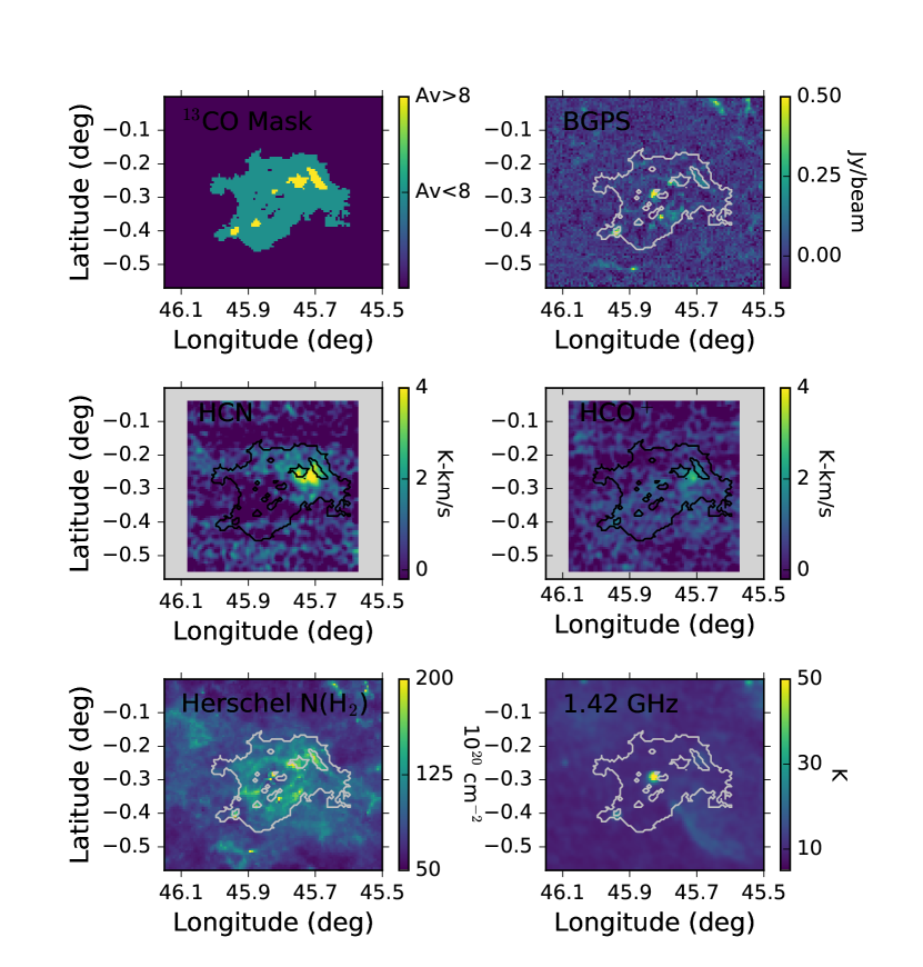
Figure 5: This figure is for the cloud G045.825$-$00.291. Except for the upper left panel, the GRS ¹³CO contours are shown in black or white, depending on the panel, along with images of other tracers or masks. Upper left is the mask for column density $\mbox{$A_{\rm V}$}\geq 8$ mag and the outermost contour of ¹³CO emission; upper right is the BGPS millimeter-wave continuum emission in color with the ¹³CO contour in white; middle left is the HCN integrated intensity in color with the ¹³CO contour in black; middle right is the HCO⁺ integrated intensity in color with the ¹³CO contour in black; lower left is the gas column density determined from Herschel in color with the ¹³CO contour in white; lower right is the 1.42 GHz radio continuum emission in color with the ¹³CO contour in white; The size of the box in the middle panels shows the region mapped in HCN and HCO⁺. The ¹³CO is in units of K km s^-1($T_{\rm mb}$) scaled 0 to 50 K km s^-1; Color bars indicate the range and scaling of the other tracers.

Figure 6: This figure is for the cloud G046.495$-$00.241. Except for the upper left panel, the GRS ¹³CO contours are shown in black or white, depending on the panel, along with images of other tracers or masks. Upper left is the mask for column density $\mbox{$A_{\rm V}$}\geq 8$ mag and the outermost contour of ¹³CO emission; upper right is the BGPS millimeter-wave continuum emission in color with the ¹³CO contour in white; middle left is the HCN integrated intensity in color with the ¹³CO contour in black; middle right is the HCO⁺ integrated intensity in color with the ¹³CO contour in black; lower left is the gas column density determined from Herschel in color with the ¹³CO contour in white; lower right is the 1.42 GHz radio continuum emission in color with the ¹³CO contour in white; The size of the box in the middle panels shows the region mapped in HCN and HCO⁺. The ¹³CO is in units of K km s^-1($T_{\rm mb}$) scaled 0 to 50 K km s^-1; Color bars indicate the range and scaling of the other tracers.

4 Results

The most compact presentation of the results is in figures 1 to 6. In each figure, all panels present the outermost contour of the velocity integrated intensity of ¹³CO emission with four tracers of dense gas (in color) superimposed: the $\mbox{$A_{\rm V}$}>8$ mag mask based on the ¹³CO column density; the millimeter-wave continuum emission from BGPS; the HCN integrated intensity; and the HCO⁺ integrated intensity. (The method used to determine the $\mbox{$A_{\rm V}$}>8$ mask is described in §5.1.) Two panels show in color the column density determined from Herschel data and the radio continuum emission.

Inspection reveals a considerable range of behavior. G034.158$+$00.147 and G034.997$+$00.330 show strong emission from both line tracers and BGPS, and all tracers agree qualitatively on the location of the dense gas. At the other extreme, G037.677$+$00.155 has only very weak emission from either dense line tracer, both concentrated in the upper right corner of the ¹³CO map; G037.677$+$00.155 has weak ¹³CO emission and no regions with $\mbox{$A_{\rm V}$}>8$ mag. G036.459$-$00.183 and G045.825$-$00.291 have weak emission from the dense line tracers that is more extended and poorly correlated with the BGPS and $\mbox{$A_{\rm V}$}>8$ mag indicators. G046.495$-$00.241 has three, often overlapping, velocity components that complicate analysis, but in general it shows moderate agreement among the various tracers of dense gas. More complete results for each cloud (spectra at peaks, contour diagrams of integrated intensity, etc.) are provided in the Appendix.

5 Analysis

5.1 Tracer Comparison

We quantify the results from the visual comparison in §4, focusing on the fraction of the luminosity of the line tracers that comes from regions indicated to be dense, based on extinction or millimeter-wave continuum emission. This section is geared toward understanding how the line tracers will behave when clouds are observed with spatial resolutions much greater than 1 pc, as in observations of other galaxies. Thus we do not separate emission from clumps that differ in spatial or velocity location. That analysis is done in §5.2.

First we describe the method used to make the maps of column density and the $\mbox{$A_{\rm V}$}>8$ mag mask. CO (our convention is that the most common isotope is indicated unless otherwise specified) and ¹³CO data were used to define column density maps for each target. The procedure to convert these data into ¹³CO column densities for this paper was largely described by Ripple et al. (2013). In short, we used equations 1-5 of Ripple et al. (2013) to calculate the column density of ¹³CO, assuming low to moderate optical depths of ¹³CO emission and optically thick CO emission. Monte Carlo simulations are computed to derive the excitation temperature and ¹³CO column density and corresponding uncertainties generated by the thermal noise of the data. We then converted to molecular hydrogen by assuming an isotopic ¹²C/¹³C ratio of 45 (Milam et al. 2005) and fractional abundance of 6000 for CO, based on a recent determination of the CO abundance by Lacy et al. (2017). Our conversion to extinction of $\mbox{$A_{\rm V}$}=1.0\mbox{${}\times 10^{-21}$}N(\mbox{{\rm H}${}_{2}$})$ is also provided by Lacy et al. (2017).

The much higher threshold of 1 g cm^-2 proposed by McKee & Tan (2003) to avoid fragmentation and favor the formation of massive stars is not probed by ¹³CO emission, so we used the column density determined from Herschel data (Marsh et al. 2017) and available at the HIGAL site: http://www.astro.cardiff.ac.uk/research/ViaLactea/.

These maps of column density were used to define the regions of column density corresponding to various thresholds used to define “dense” gas. The velocity interval of ¹³CO emission was used to limit the range of velocities of plausible emission from HCO⁺; the range was extended for HCN to account for hyperfine splitting. Then the data cubes for ¹³CO, BGPS, and Herschel column densities were convolved, resampled, and aligned with the TRAO maps. These were used to measure the luminosity inside and outside the region defined by the criterion described above. This allowed us to determine what fraction of the HCN and HCO⁺ emission arose from “dense” gas, as defined by that criterion. In this section, the main beam efficiency has been used to correct to the scale of $T_{\rm mb}$. This procedure may overestimate the brightness for very extended emission.

The luminosity inside and outside regions defining various indicators of dense gas are discussed in the following sections. The integration of luminosity is limited to the intersection of the ¹³CO-defined cloud and the mapping box from the TRAO observations for both HCN and HCO⁺, but not for ¹³CO. The equations used to compute the luminosity follow:

$$L_{X,in} =D^{2}\int dv\int d\Omega_{in} T_{X}(l,b,v),$$ (1)

and

$$L_{X,out} =D^{2}\int dv\int d\Omega_{out} T_{X}(l,b,v),$$ (2)

where $X$ refers to the tracer, $D$ is the distance in pc, and $\Omega_{in}$, and $\Omega_{out}$ are the solid angle of pixels that satisfy (in) or do not satisfy (out) one of the given conditions (column density from ¹³CO, column density from Herschel emission, or overlap with the mask of emission from the BGPS). In practice, a summed spectrum was constructed from all pixels that satisfied the conditions. The uncertainties were calculated as follows: The RMS noise of the summed spectrum ($RMS_{\rm sum}$) is the quadrature sum of RMS noise values of each pixel that satisfies the threshold condition. The uncertainty in the luminosity is then

$$RMS_{\rm L}=\delta v\sqrt{N_{\rm ch}}RMS_{\rm sum}d\Omega D^{2}$$ (3)

where $\delta v$ is the channel width and $N_{\rm ch}$ is the number of channels in the integration range. In most sources, these uncertainties were quite small compared to the luminosity, reflecting the fact that they included only the uncertainties in the summed spectrum. The distance uncertainties (Table 1) were added in quadrature for all luminosities, but not for ratios of luminosities, for which the distance cancels out.

5.1.1 Line Tracers versus the Extinction Criterion

How much of the luminosity of the line tracers arises within regions satisfying the extinction criterion ($\mbox{$A_{\rm V}$}>8$ mag)? While our main focus is on HCN and HCO⁺, we consider ¹³CO as well because its emission is stronger and easier to obtain for other galaxies.

We used the procedure described above to determine the luminosity of each tracer for regions with column density above and below that threshold, as measured by the ¹³CO column density. The values for the fraction of pixels inside the $A_{\rm V}$ criterion, the log of the total line luminosity, and the fraction of the total arising inside the $\mbox{$A_{\rm V}$}>8$ mag region ($\mbox{$f_{\rm L}$}=L_{\rm in}/L_{\rm tot}$) are listed for HCN, HCO⁺, and ¹³CO in Table 2. Two-sided errors are given for the logarithmic luminosities, which are dominated by the distance uncertainties. The distance does not enter in the $f_{\rm L}$ values, so the uncertainties are symmetric, much smaller, and given in parentheses. The mean, standard deviation, and median are given for the relevant columns. Since G037.677$+$00.155 had no pixels above the criterion, its value for $f_{\rm L}$ is zero for all three tracers. The values of $f_{\rm L}$ vary widely, with $f_{\rm L}$ between 0 and 0.54 for HCN, between 0 and 0.56 for HCO⁺, and between 0 and 0.33 for ¹³CO. HCN and HCO⁺ give very similar results for $f_{\rm L}$. In terms of the total line luminosities, the mean of the logarithms of $L_{\rm tot}$ is higher by 0.25 for HCN compared to HCO⁺. So, the two dense line tracers provide similar measures in this sample, but the luminosity of HCN is somewhat higher than that of HCO⁺. ¹³CO provides still higher luminosity, but worse correlation with the extinction criterion for the first two clouds and similar for the others.

Table 2: Line Luminosities versus $\mbox{$A_{\rm V}$}>8$

Source	$N/N_{\rm tot}$	Log $L_{\rm tot}$	$f_{\rm L}$	Log $L_{\rm tot}$	$f_{\rm L}$	Log $L_{\rm tot}$	$f_{\rm L}$
		HCN	HCN	HCO+	HCO+	13CO	13CO
G034.158+00.147	0.163	$2.68^{+0.10}_{-0.09}$	0.539 (0.003)	$2.54^{+0.10}_{-0.09}$	0.559 (0.003)	$3.75^{+0.10}_{-0.09}$	0.332 (0.000)
G034.997+00.330	0.079	$3.37^{+0.03}_{-0.04}$	0.251 (0.002)	$3.09^{+0.03}_{-0.04}$	0.243 (0.002)	$4.34^{+0.03}_{-0.04}$	0.125 (0.000)
G036.459-00.183	0.004	$2.95^{+0.06}_{-0.07}$	0.007 (0.000)	$2.81^{+0.05}_{-0.07}$	0.010 (0.000)	$3.86^{+0.05}_{-0.06}$	0.019 (0.000)
G037.677+00.155	0.000	$2.22^{+0.02}_{-0.02}$	0.000 (0.000)	$2.02^{+0.02}_{-0.02}$	0.000 (0.000)	$3.59^{+0.02}_{-0.02}$	0.000 (0.000)
G045.825-00.291	0.054	$3.13^{+0.05}_{-0.07}$	0.148 (0.003)	$2.56^{+0.05}_{-0.07}$	0.169 (0.008)	$3.88^{+0.05}_{-0.07}$	0.113 (0.001)
G046.495-00.241	0.035	$2.36^{+0.14}_{-0.17}$	0.088 (0.002)	$2.20^{+0.14}_{-0.17}$	0.098 (0.002)	$3.34^{+0.14}_{-0.17}$	0.075 (0.000)
Mean	0.056	2.79	0.172	2.54	0.180	3.79	0.111
Std Dev.	0.055	0.41	0.185	0.36	0.190	0.31	0.109
Median	0.045	2.82	0.118	2.55	0.133	3.80	0.094

Notes: 1. Units of luminosities are K km s^-1pc².

Figure 7: The fraction of line luminosity arising above $\mbox{$A_{\rm V}$}>8$ mag is plotted versus total line luminosity. HCN is plotted on the left and HCO⁺ on the right.

Does the fraction of line luminosity arising at high column density correlate with any observable properties? Figure 7 plots $f_{\rm L}$ versus total line luminosity; no trend is apparent. Neither is there a strong trend of increasing $f_{\rm L}$ with SFR (Fig. 8). While the highest values of $f_{\rm L}$ correspond to the cloud with the highest star formation rate, the other clouds do not support an overall trend.

Finally, we comment on the absence of any gas with $\mbox{$A_{\rm V}$}>8$ mag in G037.677$+$00.155. That cloud is large (27 pc) and massive (log $\mbox{$M_{\rm cloud}$}=5.45$), with the second highest SFR in the sample. The absence of regions with $\mbox{$A_{\rm V}$}>8$ mag and only weak, fragmented emission in dense gas tracers is thus surprising, except that the fraction of dense gas indicated by the BGPS emission (3.7${}\times 10^{-3}$) was the lowest in the sample. This cloud is probably more evolved, with the current episode of star formation coming to an end.

5.1.2 Line Tracers versus the 1 g cm^-2 Criterion

McKee & Tan (2003) proposed a criterion of surface density of 1 g cm^-2 for efficient formation of massive stars. The ¹³CO does not trace such high column densities, so we used the column density from the Herschel data, as described in §5.1. There is a small region (10 pixels) in G034.158$+$00.147 and a single pixel in G034.997$+$00.330 that meet the criterion. The fraction of the HCN luminosity in those regions are 0.034 for G034.158$+$00.147 and 0.006 in G034.997$+$00.330. For HCO⁺, the equivalent fractions are 0.046 and 0.006; for ¹³CO, they are 0.019 and 0.0. (For ¹³CO, no pixels were inside that region in G034.997$+$00.330, presumably because of slightly different sampling.) These numbers are interestingly small; the criterion was originally formulated in the context of the early work on dense clumps identified with strong localized emission by CS $J=7\rightarrow 6$, (Plume et al. 1997) similar in spirit to the HCN and HCO⁺ line tracers, but much more biased towards very high densities. The sample of Plume et al. (1997) was originally based on sources with water masers. As far as we know, G034.158$+$00.147  is the only source in our sanple with a water maser.

5.1.3 Line Tracers versus BGPS emission

Vutisalchavakul et al. (2016) used the millimeter-wave continuum emission from the BGPS survey to estimate the mass of dense gas. To test how well the line tracers correlate with that criterion for “dense”, we also computed the line luminosities inside and outside the mask supplied by the BGPS catalog. In the mask file, each pixel is set to zero if no emission was detected or to the catalog number of the source if emission was significant (Ginsburg et al. 2013).

Table 3: Line Luminosities versus BGPS Emission

Source	$N/N_{\rm tot}$	Log $L_{\rm tot}$	$f_{\rm L}$	Log $L_{\rm tot}$	$f_{\rm L}$	$N/N_{\rm tot}$	Log $L_{\rm tot}$	$f_{\rm L}$
	HCN	HCN	HCN	HCO+	HCO+	13CO	13CO	13CO
G034.158+00.147	0.625	$2.68^{+0.10}_{-0.09}$	0.843 (0.006)	$2.54^{+0.10}_{-0.09}$	0.865 (0.006)	0.612	$3.75^{+0.10}_{-0.09}$	0.741 (0.001)
G034.997+00.330	0.267	$3.37^{+0.03}_{-0.04}$	0.454 (0.004)	$3.09^{+0.03}_{-0.04}$	0.452 (0.004)	0.261	$4.34^{+0.03}_{-0.04}$	0.344 (0.000)
G036.459-00.183	0.205	$2.95^{+0.05}_{-0.06}$	0.336 (0.004)	$2.81^{+0.05}_{-0.06}$	0.401 (0.003)	0.235	$3.86^{+0.05}_{-0.06}$	0.347 (0.000)
G037.677+00.155	0.189	$2.22^{+0.03}_{-0.03}$	0.186 (0.008)	$2.02^{+0.02}_{-0.02}$	0.304 (0.010)	0.230	$3.59^{+0.02}_{-0.02}$	0.275 (0.001)
G045.825-00.291	0.110	$3.13^{+0.05}_{-0.07}$	0.142 (0.004)	$2.56^{+0.05}_{-0.08}$	0.184 (0.010)	0.116	$3.88^{+0.05}_{-0.07}$	0.141 (0.001)
G046.495-00.241	0.145	$2.36^{+0.14}_{-0.17}$	0.240 (0.004)	$2.20^{+0.14}_{-0.17}$	0.252 (0.004)	0.128	$3.34^{+0.14}_{-0.17}$	0.197 (0.000)
Mean	0.257	2.79	0.367	2.54	0.410	0.264	3.79	0.341
Std Dev.	0.172	0.41	0.236	0.36	0.222	0.165	0.31	0.194
Median	0.197	2.82	0.288	2.55	0.353	0.233	3.80	0.309

Notes: 1. Units of luminosities are K km s^-1pc².

As can be seen from figure 5, G045.825$-$00.291 has very little overlap between the BGPS emission and the HCN/HCO⁺ emission. Consequently, the values in the table for that source are effectively upper limits. For the remaining four sources, the correlation with BGPS is reasonably strong, as captured in $f_{\rm L}$ for BGPS in Table 3. As for the extinction criterion, the two dense line tracers agree well, but the luminosity of HCN is greater by 0.25 in the log on average. The $f_{\rm L}$ values for ¹³CO are more comparable to the dense line tracers than was the case for the extinction criterion. This reflects the fact that the BGPS emission from distant clouds traces a lower average density than it traces in nearby clouds, so that it begins to trace structures between the scale of clouds and dense clumps beyond distances of 5-10 kpc (Dunham et al. 2011). Thus, ¹³CO, HCN, and HCO⁺ all seem to trace the gas inferred from the BGPS data similarly. Since Vutisalchavakul et al. (2016) used BGPS to measure dense gas mass, we would expect that their values of SFR per unit mass would be lower than those for the nearby clouds, where the $\mbox{$A_{\rm V}$}>8$ mag criterion can be used. Indeed, this was the case.

Figure 8: The fraction of line luminosity arising in the BGPS emission region is plotted versus the star forrmation rate. HCN is plotted on the left and HCO⁺ on the right.

5.1.4 Conversion of Line Tracer Luminosity to Mass of Dense Gas

We also plot the mass of dense gas determined from BGPS versus the luminosity of HCN in figure 9 for both the total line tracer luminosity and the line tracer luminosity inside the BGPS mask. Both correlate, but the correlation is better for $L_{in}$. The values of $M_{\rm dense}$, $L_{\rm in}$, and both conversion factors $\mbox{$\alpha_{\rm in}$}=\mbox{$M_{\rm dense}$}/L_{\rm in}$ and $\mbox{$\alpha_{\rm tot}$}=\mbox{$M_{\rm dense}$}/L_{\rm tot}$ are tabulated in Table 4 for both HCN and HCO⁺, along with the means, standard deviations, and medians.

Table 4: $M_{\rm dense}$versus Luminosities

Source	Log $M_{\rm dense}$	Log $L_{\rm in}$	Log $\alpha_{\rm in}$	Log $\alpha_{\rm tot}$	Log $L_{\rm in}$	Log $\alpha_{\rm in}$	Log $\alpha_{\rm tot}$
	M⊙	HCN	HCN	HCN	HCO+	HCO+	HCO+
G034.158+00.147	$4.13^{+0.10}_{-0.09}$	$2.61^{+0.10}_{-0.09}$	$1.52^{+0.02}_{-0.02}$	$1.45^{+0.02}_{-0.02}$	$2.48^{+0.10}_{-0.09}$	$1.66^{+0.02}_{-0.02}$	$1.59^{+0.02}_{-0.02}$
G034.997+00.330	$4.08^{+0.15}_{-0.23}$	$3.03^{+0.03}_{-0.04}$	$1.05^{+0.15}_{-0.22}$	$0.71^{+0.15}_{-0.22}$	$2.74^{+0.03}_{-0.04}$	$1.34^{+0.15}_{-0.22}$	$0.99^{+0.15}_{-0.22}$
G036.459-00.183	$3.49^{+0.15}_{-0.23}$	$2.48^{+0.05}_{-0.06}$	$1.01^{+0.14}_{-0.22}$	$0.54^{+0.14}_{-0.22}$	$2.41^{+0.05}_{-0.06}$	$1.08^{+0.14}_{-0.22}$	$0.68^{+0.14}_{-0.22}$
G037.677+00.155	$3.02^{+0.16}_{-0.25}$	$1.49^{+0.02}_{-0.03}$	$1.53^{+0.16}_{-0.25}$	$0.80^{+0.16}_{-0.25}$	$1.51^{+0.02}_{-0.02}$	$1.51^{+0.16}_{-0.25}$	$0.99^{+0.16}_{-0.25}$
G045.825-00.291	$3.91^{+0.15}_{-0.24}$	$2.28^{+0.05}_{-0.07}$	$1.63^{+0.14}_{-0.22}$	$0.78^{+0.14}_{-0.22}$	$1.82^{+0.05}_{-0.07}$	$2.09^{+0.14}_{-0.22}$	$1.35^{+0.15}_{-0.22}$
G046.495-00.241	$2.85^{+0.19}_{-0.32}$	$1.74^{+0.14}_{-0.17}$	$1.11^{+0.15}_{-0.23}$	$0.49^{+0.15}_{-0.23}$	$1.60^{+0.14}_{-0.17}$	$1.25^{+0.15}_{-0.23}$	$0.65^{+0.15}_{-0.23}$
Mean	3.579	2.271	1.308	0.793	2.094	1.486	1.044
Std. Dev.	0.505	0.521	0.254	0.315	0.471	0.326	0.339
Median	3.701	2.381	1.314	0.743	2.118	1.423	0.992

Notes: 1. Units of luminosities are K km s^-1pc².

If we restrict the luminosity of HCN to the region inside the BGPS mask, we get $\mbox{$\langle\log(\mbox{$\alpha_{\rm in}$})\rangle$}=1.308\pm.254$, translating to $\mbox{$M_{\rm dense}$}=20^{+16}_{-9}$ $L({\rm HCN})$. Including the entire cloud, the result is $\mbox{$\langle\log(\mbox{$\alpha_{\rm tot}$})\rangle$}=0.793\pm.315$, translating to $\mbox{$M_{\rm dense}$}=6.2^{+6.6}_{-3.0}$ $L({\rm HCN})$. The latter value is more appropriate for extragalactic observations, where the luminosity will arise from the whole cloud if one wants to estimate the mass of material with densities similar to that of BGPS sources in the Galaxy. A conversion factor of 20 (appropriate for the luminosity inside the BGPS mask) is the same as the average of $20\pm 5$ derived by Wu et al. (2010) while the value of 6.2 is more similar to, but a bit lower than, that used in extragalactic studies (Gao & Solomon 2004; Liu et al. 2015; Jiménez-Donaire et al. 2019)

Figure 9: The mass of dense gas determined from BGPS data is plotted versus the line luminosity. HCN is plotted on the bottom and HCO⁺ on the top. The total line luminosities are on the left, the luminosity inside the BGPS mask on the right.

5.1.5 HCO⁺ versus HCN versus ¹³CO

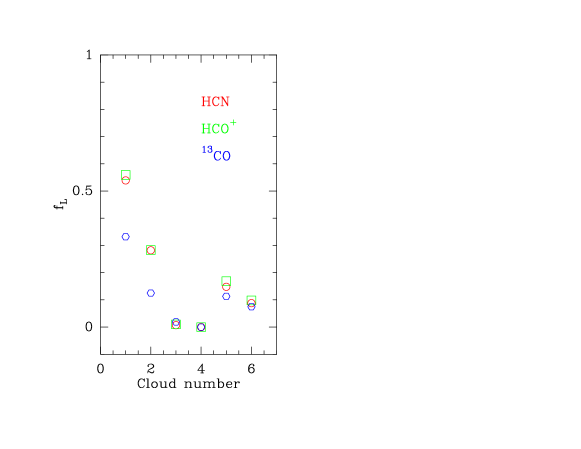
Figure 10: The fraction of luminosity ($f_{\rm L}$) within the $\mbox{$A_{\rm V}$}>8$ mag region is plotted for each tracer versus cloud number, in the order they appear in all the tables. Different symbols and colors are used to separate the different tracers.

The fraction of luminosity coming from the $\mbox{$A_{\rm V}$}>8$ mag region is plotted for each of the line tracers in figure 10. The first two clouds (G034.158$+$00.147 and G034.997$+$00.330) clearly differ from the other four. The values for $f_{\rm L}$ are higher and those for HCN or HCO⁺ clearly exceed those for ¹³CO. For the other 4, all the values are low and the different tracers are in rough agreement. In those clouds, the ¹³CO would be equally good or bad at tracing the dense gas.

The ratio of total luminosities, $\mbox{$L({\rm\mbox{{\rm HCO}${}^{+}$}})$}/\mbox{$L({\rm HCN})$}$, averaged in the logs, is 0.56, similar to the 0.7 ratio found in the EMPIRE study, (Jiménez-Donaire et al. 2019) and in the CMZ of the Galaxy (Jones et al. 2012) but there are substantial variations from cloud to cloud. Despite the differences in critical density, and probably in chemistry, the two lines seem to be tracing similar material on average in this sample. Both lines trace about the same concentration of emission, as measured by $f_{\rm L}$. For the $\mbox{$A_{\rm V}$}>8$ mag criterion, the average ratio, $\mbox{$\langle\mbox{$f_{\rm L}$}(\rm\mbox{{\rm HCO}${}^{+}$})/\mbox{$f_{\rm L}$}(\rm HCN)\rangle$}=1.14\pm 0.18$. This is not what simplistic predictions based on critical densities would have predicted (see §5.2.1 and §6).

5.2 Clump Analysis

In this section, we search for peaks, separating different velocity components where necessary. This analysis is used to characterize the spectra and sizes of the peaks identified in the line tracers. This analysis is what can be done with spatial resolution much less than 1 pc, as is common within the Galaxy.

Our standard procedure is as follows. We examine the data to find all velocity intervals with significant emission. Then we exclude those regions while removing a second-order baseline, also using only enough velocity range to get good baseline on each end ($v_{sp}$) and excluding velocities with emission ($v_{\rm win}$). The values of the total velocity range and excluded windows are shown in Table 9. Then $I$, $T_{\rm A}^{*}$ integrated over a velocity range ($v_{\rm I}$) is computed for every mapped position, regardless of whether a line is detected there. These are plotted in contour diagrams, which are used to define the peak position, find regions that should be eliminated, and find the FWHM size. Contour diagrams are made in steps of $2\sigma$, starting at $2\sigma$, where $\sigma$ is the RMS noise in the integrated intensity ($I$), as listed in Table 9. Spectra at the peak position, or in cases of weak emission, spectra averaged over nearby positions, were used to determine line properties, such as integrated intensity, velocity, line width (Table 5). This was often an iterative process in which the line properties were used to refine the velocity range ($v_{\rm I}$) for integrated intensities and the area outside the 2 $\sigma$ emission regions was refined to determine better noise levels.

Table 5: Line Fits

Source	Line	Intensity	$v$	$\Delta v$	RMS(I)	Note
		(K km s-1)	(km s-1)	(km s-1)	(K km s-1)
G034.158+00.147	HCO+	10.60	56.42 (0.02)	3.06 (0.05)	0.48
G034.158+00.147	HCN	9.84	56.60 (0.03)	2.68 (0.05)	0.48
G034.158+00.147	H13CO+	3.61	57.91 (0.09)	4.72 (0.22)	0.28
G034.158+00.147	H13CN	6.99	57.80 (0.11)	4.74 (0.25)	0.53
G034.997+00.330	HCO+	3.82	53.90 (0.03)	3.34 (0.09)	0.23
G034.997+00.330	HCN	7.19	54.50 (0.02)	3.02 (0.05)	0.30
G034.997+00.330	H13CO+	0.42	53.27 (0.14)	2.20 (0.35)	0.17
G034.997+00.330	H13CN	1.04	53.60 (0.17)	2.95 (0.39)	0.34
G036.459-00.183	HCO+	1.67	77.91 (0.06)	2.56 (0.15)	0.33
G036.459-00.183	HCN	1.72	78.50 (0.11)	2.94 (0.25)	0.33
G037.677+00.155	HCO+	1.15	82.95 (0.07)	2.52 (0.10)	0.15
G037.677+00.155	HCN	0.48	82.90 (0.21)	3.93 (0.56)	0.25
G045.825-00.291	HCO+	1.31	50.45 (0.22)	5.35 (0.56)	0.35
G045.825-00.291	HCN	2.23	50.18 (0.41)	11.1 (0.98)	0.51
G046.495-00.241	HCO+	1.20	51.35 (0.08)	2.23 (0.20)	0.11	v1
G046.495-00.241	HCN	0.96	51.20 (0.14)	2.75 (0.40)	0.15	v1
G046.495-00.241	HCO+	0.55	54.48 (0.14)	1.93 (0.34)	0.10	v2
G046.495-00.241	HCN	0.65	54.40 (0.16)	2.27 (0.57)	0.08	v2
G046.495-00.241	HCO+	1.05	58.54 (0.15)	3.05 (0.45)	0.16	v3
G046.495-00.241	HCN	1.61	58.80 (0.19)	2.21 (0.36)	0.16	v3, hfs

Notes: 1. v1 means velocity component 1. 2. hfs means fit to hyperfine components.

5.2.1 What is the origin of the line tracer luminosity from low density regions?

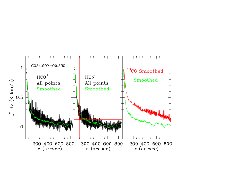
Figure 11: The integrated intensity of the HCO⁺ and HCN lines as a function of distance from the peak position of each for G034.997+00.330. The red vertical line shows the FWHM size that defines the dense core. The red horizontal line is drawn at 3 times the rms noise in the normalized intensity. The panel on the right shows the HCO⁺ and ¹³CO lines together, after Hanning smoothing by 30 points.

With clear identification of the center of emission, we can explore the origin of the luminosity of dense line tracers outside the region of the dust tracers. G034.997$+$00.330 provides a good test case because there is a single, clearly defined peak in the dense line tracers. In figure 11, the integrated intensities are sorted by distance from the peak position, normalized to the peak, and plotted versus distance; smoothed versions are also plotted. While both positive and negative values are found at large separations from the peak, there is a positive bias. In this source, the roughly 72% of the dense line tracers’ luminosity arising outside the $\mbox{$A_{\rm V}$}>8$ mag mask does not arise in secondary weak emission peaks, but in very widespread emission that is mostly below the detection threshold in individual spectra ($\mbox{$T_{\rm A}^{*}$}\sim 0.3$ K for a $3\sigma$ detection).

Having ruled out error beam contributions, we can use the spectra averaged over the whole region outside the $\mbox{$A_{\rm V}$}>8$ mag region to determine the properties of the extended emission. For all but G034.997$+$00.330, the characteristic $T_{\rm mb}$ ranges from 0.01 K to 0.03 K. If this emission is truly distributed, we can use RADEX (van der Tak et al. 2007) to determine the density of colliders needed to produce such weak lines. The results are shown in figure 12. Because the observations of HCO⁺ and HCN show nearly equal line strengths, we adjusted the abundance to produce that result. For HCO⁺, we used $N({\mbox{{\rm HCO}${}^{+}$}})=1\mbox{${}\times 10^{13}$}$ cm^-2, and for HCN, $N({\rm HCN})=2\mbox{${}\times 10^{14}$}$ cm^-2. For total column density, $N=1\mbox{${}\times 10^{21}$}$ cm^-2, corresponding to about $\mbox{$A_{\rm V}$}=1$ mag, these would correspond to $X=1\mbox{${}\times 10^{-8}$}$ for HCO⁺, and $X=2\mbox{${}\times 10^{-7}$}$ for HCN. Higher total column densities would allow lower abundances. Such abundances are not unreasonable for extinctions of a few, as indicated by figure 8 of Goldsmith & Kauffmann (2017). For both, we assumed $\mbox{$T_{\rm K}$}=20$ K and a linewidth of 1 km s^-1. These results illustrate that the low-level, very extended emission that can dominate the total luminosity can arise in gas with densities as low as 50 to 100 cm^-3. These densities are similar to the average densities ($\bar{n}$) of the entire cloud, determined by dividing the mass by the volume; for the clouds in this sample, the mean value of this average density, $\mbox{$\langle\mbox{$\bar{n}$}\rangle$}=96\pm 64$ cm^-3(Vutisalchavakul et al. 2016). This is a clear demonstration that common statements about dense gas tracers are too naive, as discussed further in §6.

5.2.2 Properties of the Dense Clumps Identified by the Line Tracers

Table 6: Clump Properties for HCN

Source	$r_{\rm dense}$	$L_{\rm dense}$	$f_{\rm L}$	$M_{\rm dv}$	$\Sigma$	$\bar{n}$	Note
	(pc)	(K km s-1 pc2)		(M⊙)	(M⊙ pc-2)	(cm-3)
G034.158$+$00.147	$0.86^{+0.16}_{-0.14}$	$94.1^{+36.2}_{-32.7}$	$0.20^{+0.07}_{-0.07}$	$2845^{+596}_{-548}$	$1237^{+259}_{-238}$	$18538^{+7163}_{-6477}$
G034.997$+$00.330	$2.01^{+0.37}_{-0.37}$	$438.9^{+169.3}_{-169.8}$	$0.21^{+0.08}_{-0.08}$	$1454^{+533}_{-533}$	$114^{+42}_{-42}$	$728^{+352}_{-352}$
G036.459$-$00.183	$3.61^{+0.39}_{-0.40}$	$246.4^{+71.2}_{-72.2}$	$0.28^{+0.08}_{-0.08}$	$3535^{+563}_{-569}$	$86^{+14}_{-14}$	$306^{+75}_{-76}$
G037.677$+$00.155	$1.74^{+0.24}_{-0.24}$	$18.4^{+7.8}_{-7.8}$	$0.11^{+0.04}_{-0.04}$	$1652^{+264}_{-264}$	$173^{+28}_{-28}$	$1274^{+367}_{-368}$
G045.825$-$00.291	$2.49^{+0.32}_{-0.34}$	$166.0^{+57.2}_{-59.6}$	$0.12^{+0.04}_{-0.04}$	$10631^{+2605}_{-2658}$	$547^{+134}_{-137}$	$2816^{+928}_{-970}$
G046.495$-$00.241	$1.12^{+0.25}_{-0.23}$	$14.4^{+6.7}_{-6.3}$	$0.06^{+0.03}_{-0.03}$	$830^{+235}_{-224}$	$211^{+60}_{-57}$	$2421^{+1148}_{-1069}$	v1
G046.495$-$00.241	$1.02^{+0.23}_{-0.21}$	$8.3^{+3.9}_{-3.6}$	$0.04^{+0.02}_{-0.01}$	$565^{+235}_{-230}$	$174^{+73}_{-71}$	$2199^{+1247}_{-1187}$	v2
G046.495$-$00.241	$1.45^{+0.31}_{-0.28}$	$37.9^{+16.4}_{-15.1}$	$0.17^{+0.07}_{-0.06}$	$2020^{+732}_{-711}$	$304^{+110}_{-107}$	$2678^{+1377}_{-1297}$	v3
Mean	1.79	128.1	0.147	2942	356	3870
Std. Dev.	0.86	141.7	0.075	3048	360	5611
Median	1.60	66.0	0.144	1836	193	2310

Note. v1, v2, etc. indicate velocity component when separated.

Table 7: Clump Properties for HCO⁺

Source	$r_{\rm dense}$	$L_{\rm dense}$	$f_{\rm L}$	$M_{\rm dv}$	$\Sigma$	$\bar{n}$	Note
	(pc)	(K km s-1 pc2)		(M⊙)	(M⊙ pc-2)	(cm-3)
G034.158$+$00.147	$0.55^{+0.14}_{-0.13}$	$56.2^{+30.3}_{-28.9}$	$0.16^{+0.09}_{-0.08}$	$1819^{+487}_{-463}$	$1936^{+518}_{-492}$	$45358^{+23133}_{-21888}$
G034.997$+$00.330	$1.82^{+0.36}_{-0.36}$	$205.7^{+89.0}_{-89.2}$	$0.17^{+0.07}_{-0.07}$	$1316^{+494}_{-495}$	$126^{+47}_{-47}$	$889^{+454}_{-455}$
G036.459$-$00.183	$6.32^{+0.54}_{-0.56}$	$681.6^{+177.7}_{-180.9}$	$1.06^{+0.26}_{-0.28}$	$6184^{+895}_{-908}$	$49^{+7}_{-7}$	$100^{+21}_{-21}$
G037.677$+$00.155	$2.52^{+0.24}_{-0.24}$	$81.7^{+18.7}_{-18.8}$	$0.66^{+0.15}_{-0.15}$	$2389^{+293}_{-294}$	$120^{+15}_{-15}$	$609^{+124}_{-124}$
G045.825$-$00.291	$3.21^{+0.34}_{-0.37}$	$150.7^{+51.3}_{-53.5}$	$0.42^{+0.14}_{-0.14}$	$13722^{+3213}_{-3286}$	$424^{+99}_{-101}$	$1690^{+501}_{-529}$
G046.495$-$00.241	$0.61^{+0.17}_{-0.16}$	$7.7^{+4.5}_{-4.3}$	$0.05^{+0.03}_{-0.03}$	$456^{+151}_{-146}$	$385^{+127}_{-123}$	$8045^{+4704}_{-4495}$	v1
G046.495$-$00.241	$1.15^{+0.25}_{-0.23}$	$8.6^{+4.1}_{-3.8}$	$0.05^{+0.02}_{-0.02}$	$638^{+265}_{-259}$	$154^{+64}_{-62}$	$1722^{+966}_{-919}$	v2
G046.495$-$00.241	$0.76^{+0.19}_{-0.18}$	$8.8^{+4.7}_{-4.5}$	$0.06^{+0.03}_{-0.03}$	$1058^{+411}_{-400}$	$580^{+225}_{-220}$	$9762^{+5701}_{-5446}$	v3
Mean	2.12	150.1	0.328	3448	472	8522
Std. Dev.	1.82	211.9	0.341	4241	580	14333
Median	1.48	69.0	0.167	1568	270	1706

Note. v1, v2, etc. indicate velocity component when separated.

In this section, we derive the properties of the dense clumps, as separated in position and velocity in order to compare them to the properties of the dense clumps studied by Wu et al. (2010). This analysis addresses the question of whether we are comparing apples to oranges. For this purpose, we follow the procedure in Wu et al. (2010). This procedure requires the integrated line intensity (I) and the linewidth ($\Delta v$) at the peak position, the FWHM angular size of the emission, and the distance.

We use the spectrum of the line at the peak, or in case of weak lines that are fairly uniformly distributed, an average over spectra surrounding the peak, to get the intensity and the linewidth. We use the linewidth from HCO⁺ or H¹³CO⁺ also for the HCN analysis to avoid issues caused by the hyperfine structure of HCN. When the lines of the H¹³CO⁺ were strong enough, we used them to get the linewidth, following Wu et al. (2010). This was possible only for G034.158$+$00.147 and G034.997$+$00.330.

We find the angular size of the source at the FWHM of the integrated intensity map. The FWHM source size is determined by plotting the 50% contour and determining the geometric mean of the two dimensions. This involves some judgment for weakly peaked regions and some “peninsulas” were ignored.

This angular size of the source, corrected for beam size, determines the properties of the dense gas, as defined by the line tracers themselves. We use equation 1 in Wu et al. (2010) to determine the line luminosity ($L_{\rm dense}$). The fraction of line tracer luminosity inside the region defined by the FWHM of the tracer, extended to a full Gaussian, was determined by dividing $L_{\rm dense}$ by the total luminosity in Table 3.

We use equation 3 of Wu et al. (2010) to compute the dense gas mass from the virial theorem ($M_{\rm dv}$). From $M_{\rm dv}$, the surface density ($\Sigma_{\rm dense}$), and volume-averaged density ($\bar{n}$) of the gas in the region defined by the line tracer are computed, using equations 5 and 6 from Wu et al. (2010). The clump properties determined from HCN are shown in Table 6, while those determined from HCO⁺ are shown in Table 7.

The distance uncertainties from Table 1 are propagated to other quantities. The virial mass is determined from the distance and linewidth; for the linewidth, the value and uncertainty from the line fits are propagated. These uncertainties also enter the uncertainties for the surface density ($\Sigma$) and average density ($\bar{n}$) of the clump. Even with possible underestimates for the uncertainties in angular size, the propagated uncertainty in the clump properties is substantial, especially for $\bar{n}$, which depends strongly on the size. Distance uncertainties were not included in ratios where the distance cancels out, such as $M_{\rm dense}$/$L_{\rm dense}$.

The means, standard deviations, and medians are given at the bottom of each table. The properties vary widely from cloud to cloud, as indicated by the very substantial standard deviations (larger or comparable to the mean values). In particular, G036.459$-$00.183 has a very large value of $r_{\rm dense}$ for HCO⁺, reflecting the very diffuse emission in that tracer; the nominal fraction of luminosity inside the Gaussian is greater than unity, while the surface and volume densities are very low. Clearly, the HCO⁺ is not tracing dense gas in this source; HCN indicates a smaller size and lower $f_{\rm L}$, leading to larger surface and volume densities, but still more characteristic of clouds than of clumps.

For comparison, Wu et al. (2010) found a median $r_{\rm dense}$ of $0.71$, a median $M_{\rm dense}$ of 2.7${}\times 10^{3}$ M_⊙, and the median $\bar{n}$ of 1.6${}\times 10^{4}$ cm^-3. The regions probed by the half-power size of line tracer emission in the current sample are larger in size, but similar in mass, and therefore lower in both surface density and mean density. The sample of Wu et al. (2010) was derived from studies originally selected by the presence of water masers, and subsequently, strong emission from CS $J=7\rightarrow 6$, so they probably represented particularly dense regions (Plume et al. 1997).

Comparing HCO⁺ and HCN, the clump properties are broadly similar. Using the full width of the half power size to define the dense clump produces similar results for the two tracers in the median, though differences can be seen in individual sources (e.g., G036.459$-$00.183). While chemical differences caused by factors like proximity to ionizing sources may well introduce differences, the two tracers produce similar results in this sample of Galactic sources.

5.2.3 Virial Parameters

Whether or not a particular region is primed to form stars depends most simply on the relative importance of turbulence versus gravity. This competition is crudely captured by the virial parameter. However, measuring the virial parameter is difficult, especially for substructures within clouds, for which boundaries are somewhat arbitrary and the contribution of surrounding material is ignored (Mao et al. 2019) It is, however, something observers can estimate.

Table 8: Virial Parameters

Source	$\alpha_{\rm dv}$(HCN)	$\alpha_{\rm dv}$(HCO+)	Note
G034.158$+$00.147	$0.21^{+0.04}_{-0.03}$	$0.13^{+0.02}_{-0.02}$
G034.997$+$00.330	$0.12^{+0.06}_{-0.06}$	$0.11^{+0.06}_{-0.06}$
G036.459$-$00.183	$1.13^{+0.47}_{-0.47}$	$2.01^{+0.83}_{-0.82}$
G037.677$+$00.155	$1.62^{+0.73}_{-0.72}$	$2.29^{+1.03}_{-1.01}$
G045.825$-$00.291	$1.35^{+0.61}_{-0.61}$	$1.72^{+0.77}_{-0.78}$
G046.495$-$00.241	$4.79^{+2.14}_{-2.11}$	$3.11^{+1.39}_{-1.37}$	1
Mean	1.54	1.56
Std. Dev.	1.56	1.10
Median	1.24	1.86

1. Combination of the three velocity components.

Table 8 presents the virial parameters, calculated from $\mbox{$\alpha_{\rm dv}$}=\mbox{$M_{\rm dv}$}/\mbox{$M_{\rm dense}$}$. For G046.495$-$00.241, the values of $M_{\rm dv}$ for the three separate velocity components have been added together for comparison to $M_{\rm dense}$, which included all the BGPS sources. For some clouds, the BGPS and dense line tracer maps agree well, but for others, the agreement is poor (cf. figures 1 to 6). Calculation of $\alpha_{\rm dv}$ for those is at best a crude indicator.

The first two sources have small values for $\alpha_{\rm dv}$. The other four sources have $\mbox{$\alpha_{\rm dv}$}\geq 1$, consistent within uncertainties with unbound structures and certainly less dominated by gravity. The spread in $\alpha_{\rm dv}$ in this sample is consistent with the range of values found for BGPS sources in general by Svoboda et al. (2016), with the first two sources lying near the lowest 10% point of the distribution (Table 7 of Svoboda et al. 2016), but our median values are higher than those for the full BGPS sample.

6 Discussion

6.1 The Concept of a Dense Gas Tracer

The idea that certain molecules are tracers of dense gas has its origin in the early days of molecular line astronomy. At that time, sensitivities were poor, maps were small, and thus the maps of dense gas line tracers were much smaller than those of CO and ¹³CO. Studies of multiple transitions of molecules like CS and H₂CO provided evidence for gas with densities of about $n\sim\mbox{$10^{5}$}$ cm^-3(Snell et al. 1984; Mundy et al. 1986, 1987). These studies and many others led to the naive idea that a single line of these molecules indicated the presence of gas of a certain density, often described as the critical density.

The idea of a critical density arose among radio astronomers when most observations were at centimeter wavelengths, for which the Rayleigh-Jeans limit is appropriate. In that limit, the excitation temperature of a line increases from the background temperature of about 2.73 K up the kinetic temperature over a wide range of densities . By balancing spontaneous radiative decay and collisional de-excitation, a “critical” density can be defined. As discussed in detail by Evans (1989) the critical density in the R-J limit lies near the low density limit , just as the excitation temperature begins to rise above the background, but the critical density instead lies near the high density end of the range, near thermalization, for millimeter-wave lines, where the R-J approximation is not valid. Consequently, for millimeter-wave lines, almost all emission arises from gas well below the critical density, commonly called sub-thermal emission. Thus, even for the simplified two-level molecule, the idea that a particular line arises in gas above the critical density of that line is incorrect.

Once one drops the two-level approximation, considers collisions to higher levels, and includes trapping, lines can be appreciably excited at even lower densities. To make this point, Evans (1999) introduced the concept of the effective density: the density needed to produce a line of $\mbox{$T_{\rm mb}$}=1$ K. Shirley (2015) explored these issues in greater detail and computed effective densities (now for the integrated intensity of 1 K km s^-1) for many transitions, confirming that many are orders of magnitude less than the corresponding critical densities. The largest discrepancies between effective and critical densities occur for the resonance transitions, $J=1\rightarrow 0$, which are the ones used in extragalactic studies and in this paper.

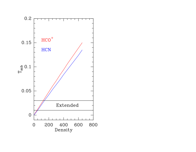
Figure 12: The main beam temperature is plotted versus the density of colliding particles, with HCO⁺ in red and HCN in blue. Typical observations in the regions outside the $\mbox{$A_{\rm V}$}>8$ mag regions are shown as horizontal lines.

To properly interpret maps of very large regions of clouds in our Galaxy and observations of other galaxies, it is important to ask what is the effective density that can produce the distributed emission As shown in figure 12, for the $J=1\rightarrow 0$ lines of HCN and HCO⁺, the entire molecular cloud, at densities of 50 to 100 cm^-3 and column densities corresponding to $\mbox{$A_{\rm V}$}\approx 1$ can produce weak emission . We have considered only collisions with H₂ and He. Electron collisions may be important for low extinction regions of the cloud, further increasing the emission at low neutral densities (Goldsmith & Kauffmann 2017). Weak emission ($\mbox{$T_{\rm A}^{*}$}=0.02-0.1$ K) in the HCO⁺  $J=1\rightarrow 0$ line from diffuse clouds ($n\approx 100$ cm^-3) was observed some time ago (Liszt & Lucas 1994). In most cases, the area of this weak emission is large enough that its weak emission dominates the regions of truly dense gas in determining the total luminosity of the line tracer.

We must now ask if there is any remaining validity to using dense gas tracers. The answer depends on the use we make of them. We cannot say that they “probe only the dense gas,” but their emission does concentrate into the dense regions better than CO or ¹³CO (see figure 11). Star formation rates are predicted more consistently from nearby clouds to distant galaxies using the still loosely defined dense gas than from using CO (Vutisalchavakul et al. 2016). Lines from higher $J$ levels will be more strongly biased toward denser gas, but are harder to observe.

6.2 Comparison to Other Work

As the $J=1\rightarrow 0$ transition of HCN became more accepted as a probe of dense gas in the extragalactic community, a number of studies began to examine the origin of HCN (and other putative tracers of dense gas) in molecular clouds in the Galaxy. We compare our results to those of other studies in this section.

Pety et al. (2017) mapped a number of molecular lines in Orion B. They found small fractions of the luminosity of HCN (18%) and HCO⁺ (16%) coming from regions with $\mbox{$A_{\rm V}$}>15$ mag. They stated that “The common assumption that lines of large critical densities ($\approx\mbox{$10^{5}$}$ cm^-3) can only be excited by gas of similar density is clearly incorrect.” Instead, they conclude that HCN and HCO⁺ mostly trace densities from 500 to 1500 cm^-3. They note that the tracer that is most strongly concentrated to the densest gas is N₂H⁺, because of chemistry.

Kauffmann et al. (2017) mapped HCN $J=1\rightarrow 0$ toward Orion A. They found that it mainly traced gas with $\mbox{$A_{\rm V}$}\approx 6$ mag, or $n\approx 870$ cm^-3. They agreed that N₂H⁺ was the best tracer of truly dense gas. They also limited the conversion factor: $\mbox{$M_{\rm dense}$}\leq 20\mbox{$L({\rm HCN})$}$, the same as our average value.

Shimajiri et al. (2017) mapped the $J=1\rightarrow 0$ transitions of HCN, HCO⁺, and their rarer isotoplogues in the nearby clouds, Aquila, Ophiuchus, and Orion B. They found that HCN and HCO⁺ lines traced the gas down to $\mbox{$A_{\rm V}$}\approx 2$ or $n\approx 1\mbox{${}\times 10^{3}$}$ cm^-3. They found that the conversion factors ($\alpha_{\rm tot}$) anti-correlated with the local FUV field strength.

Our results are broadly consistent with these works and extend their conclusions into the inner Galaxy. By considering the far outer regions of clouds without detections at individual positions, we show that even lower intensity levels may dominate the total luminosity of a cloud in these lines. Simple calculations reveal that even at densities of about 100 cm^-3, emission, albeit at very low intensities, can rival, or even dominate, the more intense emission from the truly dense regions in detemining the total luminosity of dense line tracers.

7 Conclusions

The main conclusions can be summarized as follows.

1. The correlation between different tracers of dense gas (extinction, millimeter-wave continuum emission, HCN, HCO⁺) varies from cloud to cloud.

2. Broadly, the clouds divide into two groups, one for which the dense line tracers are strong and concentrated, and the other for which they are weak and distributed.

3. In clouds where the dense line tracers are sharply peaked, all the tracers show general agreement and are more concentrated than is the ¹³CO emission.

4. In clouds with only weak, distributed emission from dense line tracers, the agreement is poor and ¹³CO traces similar material.

5. Even when the agreement is good, a substantial fraction of the line luminosity arises outside the dust-based measures of dense gas.

6. The agreement of dense line tracers with millimeter-wave continuum emission is better than the agreement for $\mbox{$A_{\rm V}$}>8$ mag. At the distances of some of these clouds, the millimeter-wave continuum emission from BGPS is typically tracing lower density gas.

7. Measurements of $L(\rm HCN)$ toward other galaxies will likely include a large fraction of emission from relatively low density gas, unless the other galaxy is a starburst galaxy. This variation may be responsible for some of the observed scatter between galaxies in the study of Jiménez-Donaire et al. (2019).

8. The conversion from luminosity to mass of dense gas, as measured by extinction or millimeter-wave continuum emission, is quite variable. For the dense regions, the conversion factor is about 20, while it is closer to 6 if the line luminosity of the whole cloud is included.

9. For this sample, HCN and HCO⁺ seem to probe about the same material. They are equally good (or bad) tracers.

10. The regions probed in this paper in HCN and HCO⁺ in two clouds in the sample are similar to those originally studied by Wu et al. but somewhat larger and less dense. The regions probed in the other clouds are substantially more diffuse and less clearly bound.

11. The distributed emission of HCN and HCO⁺ can arise from regions of very low density, $n=50-100$ cm^-3. Because of the large area of most clouds at such low densities, these less dense regions can dominate the total luminosity of line tracers.

Table 9: Reduction Details

Source	Line	$v_{\rm sp}$	$v_{\rm win}$	$v_{\rm I}$	Peak Offset	Range	Notes
		(km s-1)	(km s-1)	(km s-1)	(arcsec)	(arcsec)
G034.158+00.147	HCO+	20, 100	52, 70	52, 70	27, 10	$-$200, 160; $-$220, 140
G034.158+00.147	HCN	20, 100	40, 80	40, 80	20, 4	$-$300, 280; $-$280, 240
G034.158+00.147	H13CO+	20, 100	52, 70	52, 70	31, 29	$-$80, 120; $-$80, 140
G034.158+00.147	H13CN	20, 100	40, 80	45, 70	27, 20	$-$80, 100; $-$80, 100
G034.997+00.330	HCO+	20, 80	40, 65	40, 65	$-$20, 110	$-$220, 140; $-$160, 220
G034.997+00.330	HCN	20, 80	42, 63	42, 60	$-$20, 110	$-$220, 140; $-$160, 220
G034.997+00.330	H13CO+	20, 80	45, 60	45, 60	$-$20, 110	$-$80, 20 ;80, 160
G034.997+00.330	H13CN	20, 80	42, 63	42, 63	$-$20, 110	$-$80, 20 ;80, 160
G036.459$-$00.183	HCO+	20, 120	45, 85	68, 95	$-$61, $-$32	$-$160, 80; $-$200, 380
G036.459$-$00.183	HCN	20, 120	43, 93	67, 93	$-$20, $-$20	$-$100, 180; $-$160, 340
G037.677+00.155	HCO+	20, 120	40, 50; 75, 90	77, 88	$-$98, $-$156	$-$180, 120; $-$240, 0
G037.677+00.155	HCN	20, 120	40, 50; 73, 93	73, 93	$-$40, $-$120	$-$160, 240; $-$700, 20
G045.825$-$00.291	HCO+	20, 80	45, 65	45, 65	$-$418, 60	$-$500, $-$180; 20, 180
G045.825$-$00.291	HCN	20, 80	45, 65	40, 65	$-$400, 80	$-$480, $-$220; $-$20, 220
G046.495$-$00.241	HCO+	20, 100	40,70	47, 53	87, 3	$-$20, 120; $-$60 200	1
G046.495$-$00.241	HCN	20, 100	40,70	47, 53	83, 13	$-$60, 140; $-$40 80	1
G046.495$-$00.241	HCO+	20, 100	40,70	53, 56	$-$63, 74	$-$140, 340; 0, 120	2
G046.495$-$00.241	HCN	20, 100	40,70	53, 56	276, 150	$-$140, 340; $-$60,200	2
G046.495$-$00.241	HCO+	20, 100	40,70	56, 60	$-$307,104	$-$540, $-$140; $-$20, 200	3
G046.495$-$00.241	HCN	20, 100	40,70	56, 65	$-$292,109	$-$540, 300; $-$60, 200	3

Notes: 1. Position of center peak, velocity component v1 2. Position of eastern peak, velocity component v2 3. Position of western peak

Appendix A G034.158$+$00.147

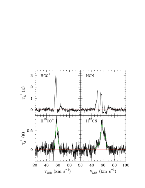
Figure 13: The spectra of HCO⁺, HCN, H¹³CO⁺, and H¹³CN toward the peak of G034.158$+$00.147. In each plot, the red line shows the zero level. For the rare isotopologues, the green line shows the fit to the line.

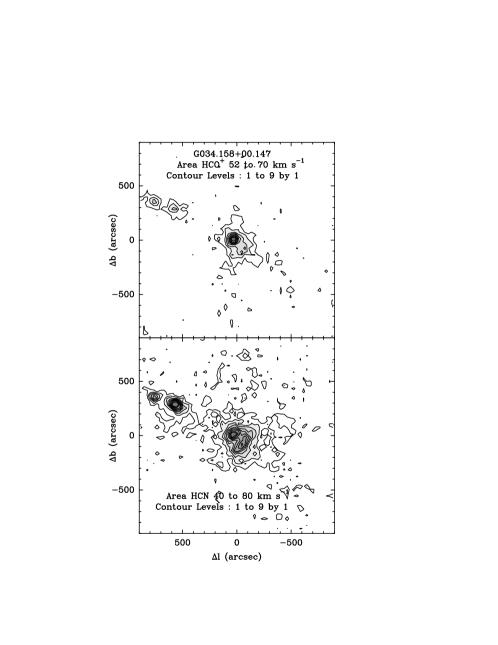
Figure 14: The integrated intensities of the HCO⁺ (top) and HCN (bottom) lines in G034.158$+$00.147. The integration is over the range of 52 to 70 km s^-1 for HCO⁺ and 40 to 80 km s^-1 for HCN.

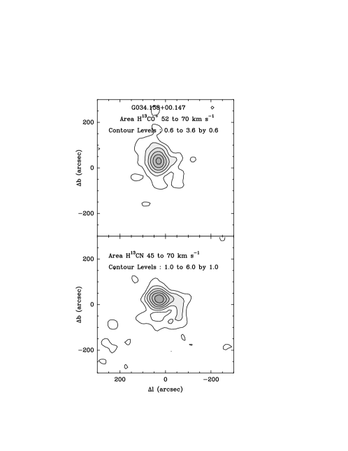
Figure 15: The integrated intensities of the H¹³CO⁺ (top) and H¹³CN (bottom) lines in G034.158$+$00.147. The integration is over the range of 52 to 70 km s^-1 for H¹³CO⁺ and 40 to 80 km s^-1 for H¹³CN.

Our map was centered, not on the source name position, but on $l=34.250$, $b=0.150$, near the H II region, G34.26+0.15. This cloud has been studied extensively under other names. The clumps to the “NE” in our maps are associated with the IRDC 34.43$+$0.24, in which Rathborne et al. (2006) identified 9 millimeter continuum sources. These are blended into two clumps in the HCN/HCO⁺ maps. G34.26$-$0.15 is a well-known star-forming region with a water maser (Hofner & Churchwell 1996) and a methanol maser (Breen et al. 2015; Kim et al. 2019).

The near kinematic distance is 3.7 kpc (Anderson et al. 2014). A VERA parallax measurement (Kurayama et al. 2011) of a water maser found by Wang et al. (2006) gives the distance as $1.56^{+0.12}_{-0.11}$ kpc, but Kurayama et al. (2011) note that the cloud would then have a peculiar velocity of about 40 km s^-1. Because this seems unlikely, we follow other recent work in using the kinematic distance. IRDC G034.43+00.24 has a polarization map (Soam et al. 2019).

The BGPS millimeter continuum emission is shown in figure 1. The maps of integrated intensity peak about 25″ east (higher $l$) of the reference position, essentially on top of the H II region. Both HCN and HCO⁺ show self-absorption and even absorption below zero around 60 km s^-1, while the H¹³CO⁺ spectrum shows a clear peak at somewhat higher velocities than those of the main lines (Fig. 13), and the isotopologues peak slightly north of the main lines. The HCN line is particularly badly affected by absorption. We attribute this effect to actual absorption of the continuum from the H II region, which has been subtracted out by the baseline process. Similar continuum absorption has been seen in HCO⁺ $J=1\rightarrow 0$ and HCN $J=3\rightarrow 2$ by Liu et al. (2013), who interpret the line profiles as a signature of infall at about 3 km s^-1. Mookerjea et al. (2007) measured a continuum of 6.7 Jy at 2.8 mm in a source size of 1$\farcs$6 by 1$\farcs$4. This would produce a continuum temperature in our 58″ beam of $3.5(2.8/3.4)^{a}$ K, where $a$ is the spectral index between the two wavelengths. Because both free-free and dust continuum emission are contributing in this spectral region, the value of $a$ is uncertain, but the wavelengths are close enough that it makes little difference. There is clearly sufficient continuum emission to explain the absorption that we observe. For extragalactic observations, these issues would not be recognized.

To determine core properties, we used the peak integrated intensity from the fit to the emission and linewidths from fits to the isotopic lines. For the HCN line properties (Table 5), we used the area within the window of 43 to 70 km s^-1, because the hyperfine and the velocity and the absorption made fits impossible. The H¹³CN line for peak 1 was fitted with hyperfine components.

Appendix B G034.997$+$00.330

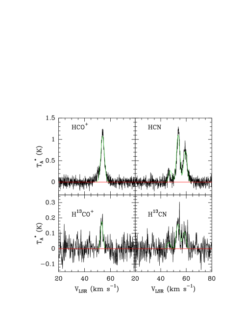
Figure 16: Top: The spectra of the HCO⁺ and HCN lines at $(-20,100)$ for source G034.997$+$00.330. The HCN shows a fit to the hyperfine structure. Bottom: The average spectrum of the H¹³CO⁺ and H¹³CN lines averaged over the nine positions around $(-20,100)$. The H¹³CN line was fitted with hyperfine structure. In each plot, the red line shows the zero level and the green line shows the fit.

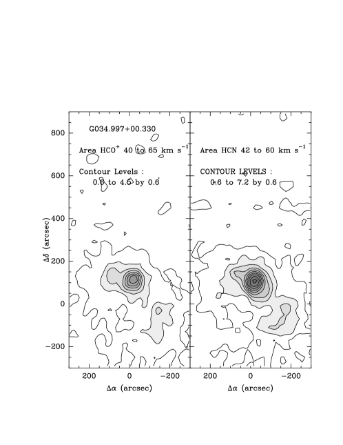
Figure 17: The integrated intensities of the HCO⁺ and HCN lines in G034.997+00.330. The integration is over the range of 45 to 60 kms for HCO⁺ and 43 to 65 km s^-1 for HCN.

This cloud was mapped in equatorial coordinates with center position $\alpha_{2000}=18^{h}54^{m}01\fs 83$, $\delta_{2000}=01\arcdeg 59\arcmin 18\farcs 0$. The BGPS millimeter continuum emission is shown in figure 2. The spectra at the peaks indicated in Table 9 are shown in figure 16. There is a single velocity component at about 57 km s^-1. The HCN line is well fitted with hyperfine components. The H¹³CO⁺ and H¹³CN lines are about 10% of the main lines, indicating only modest optical depth. Nonetheless, we use the H¹³CO⁺ line averaged over its detected region for the linewidth in computing virial mass, etc.

The contour diagrams of integrated intensity are shown in figure 17. The BGPS, HCN, and HCO⁺ emission regions correspond well. However, there is significant emission at large distances from the peak of the emission. The plots of integrated intensity of HCO⁺ and HCN versus distance from the peak are shown in figure 11. The right-most panel shows the smoothed HCO⁺ along with that from ¹³CO.

Appendix C G036.459$-$00.183

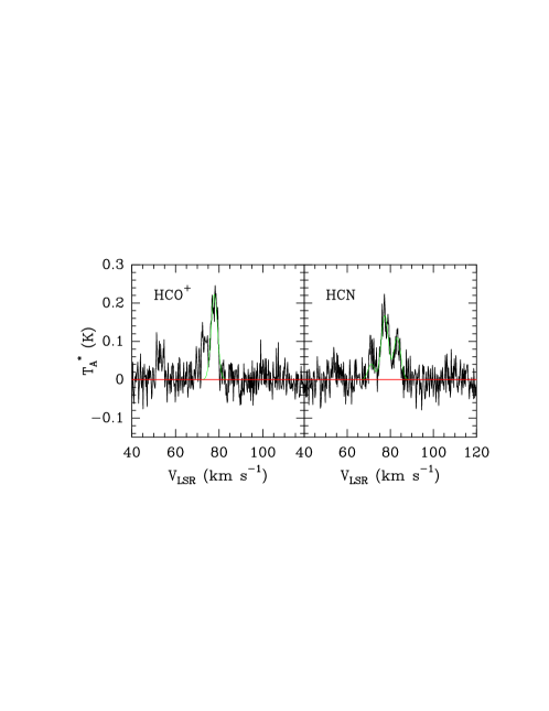
Figure 18: The spectra of HCO⁺and HCN toward the peak of G036.459$-$00.183. In each plot, the red line shows the zero level and the green line shows the fit to the line.

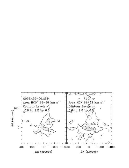
Figure 19: The integrated intensities of the HCO⁺ and HCN lines for the 78 km s^-1 component in G036.459$-$00.183.

This cloud was mapped in equatorial coordinates with center position $\alpha_{2000}=18^{h}58^{m}31\fs 78$, $\delta_{2000}=03\arcdeg 03\arcmin 18\farcs 2$. The BGPS millimeter continuum emission is shown in figure 3. The spectra are shown in figure 18. Neither the H¹³CO⁺ nor the H¹³CN lines were detected at any position. This cloud has a primary component at about 73 km s^-1,which is associated with the H II region, based on the recombination line velocity. A secondary component at about 55 km s^-1 appears in the spectrum but it is not related to this cloud, so we do not analyze it. The two components nearly overlap, but are separable at about 67 to 68 km s^-1. The hyperfine structure was used to fit the HCN lines, but the integrated intensity was integrated over all hyperfine components.

The maps of HCO⁺ and HCN are shown in figure 19. The HCO⁺ and HCN integrated intensity generally map similarly, though there are clearly differences in detail. The emission is not well peaked, and the half-power contour is nearly as large as the region of detected emission, so the properties are poorly defined.

Appendix D G037.677$+$00.155

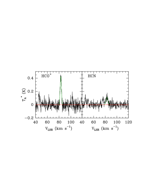
Figure 20: The spectra of HCO⁺and HCN toward their peaks in G037.677$+$00.155. The HCO⁺ line is at position $(-100,-160)$; the HCN line is an average of the 9 positions surrounding offset $(-40,-120)$. The HCN line was not well fitted with hyperfine structure so only the main peak was fitted. Note that the peak positions are somewhat different for the two species. In each plot, the red line shows the zero level and the green line shows the fit to the line.

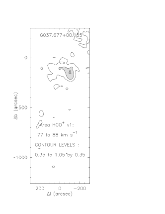
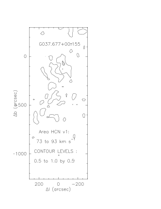
Figure 21: The integrated intensities of the HCO⁺ and HCN lines in G037.677+00.155 are shown for the velocity component near $82$ km s^-1.

This source was mapped in galactic coordinates centered on the source name position, $l=37.677$, $b=0.155$. The BGPS millimeter continuum emission is shown in figure 4. There are at least two velocity components, one near 45 km s^-1 and one near 83 km s^-1. The second one is near the velocity of the radio recombination line for this HII region, so we focus on that. Figure 20 shows the spectra. Nine positions around a nominal peak were averaged for HCN to produce the spectrum. The data were not well fitted with hyperfine structure, so we isolated the velocities around 83 km s^-1 to be fitted.

The HCO⁺ and HCN integrated intensity maps (figure 21) show extended weak emission so the peaks are not well defined. The peaks of the two lines differ. The weak emission is surprising because the cloud is relatively massive and has a substantial star formation rate and mass of dense gas, based on the submillimeter continuum data. However, the cloud was difficult to define as it exists in a region of considerable line confusion in ¹³CO.

Appendix E G045.825$-$00.291

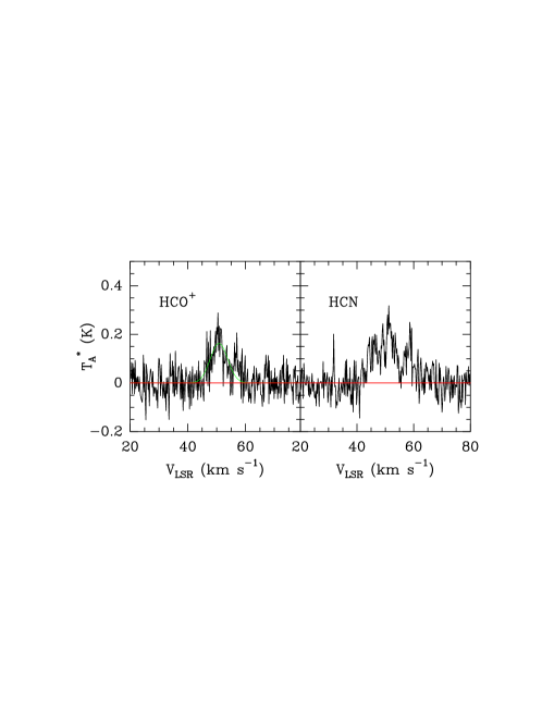
Figure 22: The spectra of HCO⁺ and HCN toward their peaks in G045.825$-$00.291. The HCO⁺ line is is an average of the 9 positions surrounding offset $(-420,60)$; the HCN line is an average of the 9 positions surrounding offset $(-400,80)$. The HCN line was not well fitted with hyperfine structure. Note that the peak positions are somewhat different for the two species. In each plot, the red line shows the zero level and the green line shows the fit to the line.

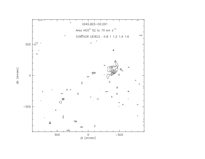
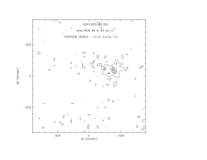
Figure 23: The integrated intensities of the HCO⁺ and HCN lines for both components in G045.825$-$00.291are shown.

This source was mapped in galactic coordinates centered on the source name position, $l=45.825$, $b=-0.291$ The BGPS millimeter continuum emission is shown in figure 5. There are several peaks in the BGPS data. Only the “northwest” one of these shows up in the HCO⁺/HCN maps (figure 23).

This source has two velocity components that are barely separable in HCO⁺ and difficult to separate in HCN. Both HCO⁺ and HCN lines are weak, but HCN is a bit stronger in integrated intensity. Figure 22 shows the spectra. We average over the 9 positions around the peak to improve the noise since the lines are very similar. Since both velocity features peak in the same area, we include both in the maps of intensity. The isotopologue lines were not detected and did not provide useful constraints on optical depth. We plot the contours of emission for both main species (Fig. 23); the peaks are slightly different for the two species, but generally consistent.

For HCO⁺ and HCN, we use the velocity width and area of the 50.5 km s^-1 feature to compute virial mass, etc. However, the HCN is confused by the hyperfine structure.

Appendix F G046.495-00.241

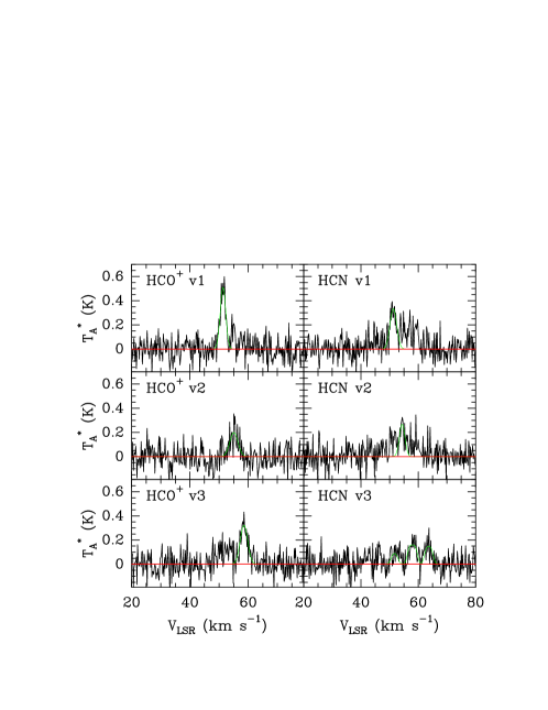
Figure 24: The spectra of HCO⁺ and HCN toward the peaks for each velocity component in G046.495$-$00.241. The positions are those nearest the peak positions listed in Table 9. The HCN lines for the first two velocity components were not well fitted with hyperfine structure so a single Gaussian was fitted to the main peak. In each plot, the red line shows the zero level and the green line shows the fit to the line.

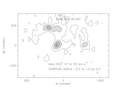
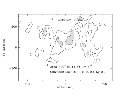
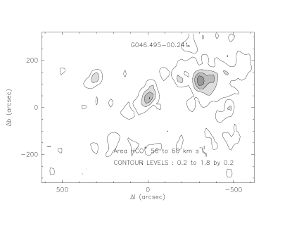
Figure 25: The integrated intensities of the HCO⁺  lines in G046.495-00.241 are shown for the three different velocity components.

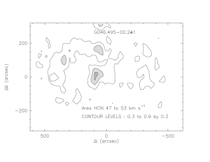
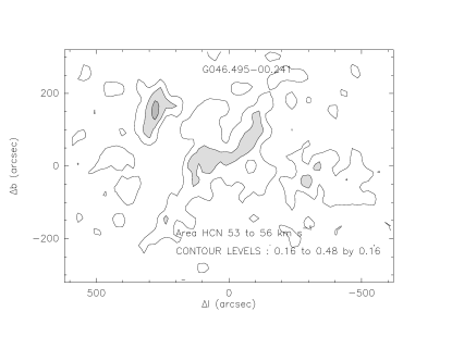
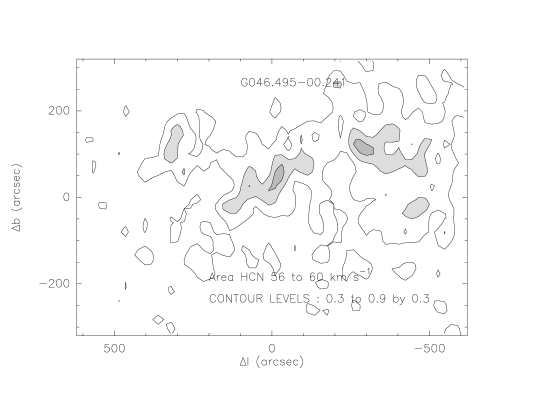
Figure 26: The integrated intensities of the HCN lines in G046.495-00.241 are shown for the three different velocity components.

This source was mapped in galactic coordinates centered, not on the source name, but on $l=46.400$, $b=-0.241$, because the source name was that of a millimeter-wave continuum source in the eastern part of the cloud. The BGPS millimeter continuum emission is shown in figure 6. There are three regions of continuum emission, which we refer to as west, central, and east in order of increasing longitude. Both HCO⁺ and HCN appear to have several velocity components (Fig. 24) and three separated emission regions when the emission is integrated over all velocities, which correspond roughly to the continuum peaks. There were no detections of the ¹³C isotopologues, so we concluded that the velocity structure was unlikely to be caused by self-absorption.

It was possible to separate the three velocity components in HCO⁺ and to make contour maps. The maps of integrated intensity are shown in figure 25. The spectra at the peaks of each component are shown in figure 24. The lowest velocity component, v1, peaks most strongly on the central peak, but has secondary peaks to the north and west that do not correspond exactly to the peaks of the other components, but overlap with them. The middle velocity component (v2) emits over an extended region, but weakly, with no strong peaks. We picked the most central and largest in size peak, which is south and east of the peak of v1. The highest velocity component denoted v3, peaks most strongly on the western (lower $l$) peak, but has secondary maxima near the other peaks. The other lines are largely absent from the western peak. Because the individual velocity components are narrow, the rms in the integrated intensity is small, so it is possible to draw more contours. The secondary peaks and extended plateaus are reflected in the secondary maxima, but the main peak is reasonable well defined. The separation for HCN is more difficult because of the hyperfine structure, so we used the velocity intervals from the HCO⁺ analysis for components v1 and v2. The hyperfine structure was more visible and separate for v3, so we fit that component. The separation into velocity components would not be possible in observations of other galaxies. The contour maps for each species and component in (fig. 26) for each component indicate the complexity of overlapping regions.

References

- Aguirre et al. (2011) Aguirre, J. E., Ginsburg, A. G., Dunham, M. K., et al. 2011, ApJS, 192, 4, doi: 10.1088/0067-0049/192/1/4
- Anderson et al. (2014) Anderson, L. D., Bania, T. M., Balser, D. S., et al. 2014, ApJS, 212, 1, doi: 10.1088/0067-0049/212/1/1
- Barnes et al. (2016) Barnes, P. J., Hernandez, A. K., O’Dougherty, S. N., Schap, III, W. J., & Muller, E. 2016, ApJ, 831, 67, doi: 10.3847/0004-637X/831/1/67
- Barnes et al. (2011) Barnes, P. J., Yonekura, Y., Fukui, Y., et al. 2011, ApJS, 196, 12, doi: 10.1088/0067-0049/196/1/12
- Breen et al. (2015) Breen, S. L., Fuller, G. A., Caswell, J. L., et al. 2015, MNRAS, 450, 4109, doi: 10.1093/mnras/stv847
- Bron et al. (2018) Bron, E., Daudon, C., Pety, J., et al. 2018, A&A, 610, A12, doi: 10.1051/0004-6361/201731833
- DeLucia & Gordy (1969) DeLucia, F., & Gordy, W. 1969, Physical Review, 187, 58, doi: 10.1103/PhysRev.187.58
- Dobbs et al. (2011) Dobbs, C. L., Burkert, A., & Pringle, J. E. 2011, MNRAS, 413, 2935, doi: 10.1111/j.1365-2966.2011.18371.x
- Dunham et al. (2011) Dunham, M. K., Rosolowsky, E., Evans, II, N. J., Cyganowski, C., & Urquhart, J. S. 2011, ApJ, 741, 110, doi: 10.1088/0004-637X/741/2/110
- Evans (1989) Evans, Neal J., I. 1989, Rev. Mexicana Astron. Astrofis., 18, 21
- Evans (1999) Evans, II, N. J. 1999, ARA&A, 37, 311, doi: 10.1146/annurev.astro.37.1.311
- Evans et al. (2014) Evans, II, N. J., Heiderman, A., & Vutisalchavakul, N. 2014, ApJ, 782, 114, doi: 10.1088/0004-637X/782/2/114
- Gao & Solomon (2004) Gao, Y., & Solomon, P. M. 2004, ApJ, 606, 271, doi: 10.1086/382999
- Ginsburg et al. (2013) Ginsburg, A., Glenn, J., Rosolowsky, E., et al. 2013, ApJS, 208, 14, doi: 10.1088/0067-0049/208/2/14
- Goldsmith & Kauffmann (2017) Goldsmith, P. F., & Kauffmann, J. 2017, ApJ, 841, 25, doi: 10.3847/1538-4357/aa6f12
- Heiderman et al. (2010) Heiderman, A., Evans, II, N. J., Allen, L. E., Huard, T., & Heyer, M. 2010, ApJ, 723, 1019, doi: 10.1088/0004-637X/723/2/1019
- Helfer & Blitz (1997) Helfer, T. T., & Blitz, L. 1997, ApJ, 478, 233, doi: 10.1086/303774
- Hofner & Churchwell (1996) Hofner, P., & Churchwell, E. 1996, A&AS, 120, 283
- Jackson et al. (2006) Jackson, J. M., Rathborne, J. M., Shah, R. Y., et al. 2006, ApJS, 163, 145, doi: 10.1086/500091
- Jeong et al. (2019) Jeong, G.-I., Kang, H., Jung, J., et al. 2019, Journal of the Korean Astronomical Society, 52, 227. https://doi.org/10.5303/JKAS.2019.52.6.227
- Jiménez-Donaire et al. (2019) Jiménez-Donaire, M. J., Bigiel, F., Leroy, A. K., et al. 2019, ApJ, 880, 127, doi: 10.3847/1538-4357/ab2b95
- Jones et al. (2012) Jones, P. A., Burton, M. G., Cunningham, M. R., et al. 2012, MNRAS, 419, 2961, doi: 10.1111/j.1365-2966.2011.19941.x
- Kauffmann et al. (2017) Kauffmann, J., Goldsmith, P. F., Melnick, G., et al. 2017, A&A, 605, L5, doi: 10.1051/0004-6361/201731123
- Kim et al. (2019) Kim, W.-J., Kim, K.-T., & Kim, K.-T. 2019, ApJS, 244, 2, doi: 10.3847/1538-4365/ab2fc9
- Kruijssen et al. (2018) Kruijssen, J. M. D., Schruba, A., Hygate, A. e. P. S., et al. 2018, MNRAS, 479, 1866, doi: 10.1093/mnras/sty1128
- Kurayama et al. (2011) Kurayama, T., Nakagawa, A., Sawada-Satoh, S., et al. 2011, PASJ, 63, 513, doi: 10.1093/pasj/63.3.513
- Lacy et al. (2017) Lacy, J. H., Sneden, C., Kim, H., & Jaffe, D. T. 2017, ApJ, 838, 66, doi: 10.3847/1538-4357/aa6247
- Lada et al. (2012) Lada, C. J., Forbrich, J., Lombardi, M., & Alves, J. F. 2012, ApJ, 745, 190, doi: 10.1088/0004-637X/745/2/190
- Lada et al. (2010) Lada, C. J., Lombardi, M., & Alves, J. F. 2010, ApJ, 724, 687, doi: 10.1088/0004-637X/724/1/687
- Liszt & Lucas (1994) Liszt, H. S., & Lucas, R. 1994, ApJ, 431, L131, doi: 10.1086/187490
- Liszt & Pety (2016) Liszt, H. S., & Pety, J. 2016, ApJ, 823, 124, doi: 10.3847/0004-637X/823/2/124
- Liu et al. (2015) Liu, L., Gao, Y., & Greve, T. R. 2015, ApJ, 805, 31, doi: 10.1088/0004-637X/805/1/31
- Liu et al. (2013) Liu, T., Wu, Y., & Zhang, H. 2013, ApJ, 776, 29, doi: 10.1088/0004-637X/776/1/29
- Mao et al. (2019) Mao, S. A., Ostriker, E. C., & Kim, C.-G. 2019, arXiv e-prints, arXiv:1911.05078. https://arxiv.org/abs/1911.05078
- Marsh et al. (2017) Marsh, K. A., Whitworth, A. P., Lomax, O., et al. 2017, MNRAS, 471, 2730, doi: 10.1093/mnras/stx1723
- McKee & Tan (2003) McKee, C. F., & Tan, J. C. 2003, ApJ, 585, 850, doi: 10.1086/346149
- Milam et al. (2005) Milam, S. N., Savage, C., Brewster, M. A., Ziurys, L. M., & Wyckoff, S. 2005, ApJ, 634, 1126, doi: 10.1086/497123
- Mookerjea et al. (2007) Mookerjea, B., Casper, E., Mundy, L. G., & Looney, L. W. 2007, ApJ, 659, 447, doi: 10.1086/512095
- Mundy et al. (1987) Mundy, L. G., Evans, Neal J., I., Snell, R. L., & Goldsmith, P. F. 1987, ApJ, 318, 392, doi: 10.1086/165376
- Mundy et al. (1986) Mundy, L. G., Snell, R. L., Evans, Neal J., I., Goldsmith, P. F., & Bally, J. 1986, ApJ, 306, 670, doi: 10.1086/164377
- Nguyen-Luong et al. (2016) Nguyen-Luong, Q., Nguyen, H. V. V., Motte, F., et al. 2016, ApJ, 833, 23, doi: 10.3847/0004-637X/833/1/23
- Nguyen-Luong et al. (2020) Nguyen-Luong, Q., Nakamura, F., Sugitani, K., et al. 2020, ApJ, 891, 66, doi: 10.3847/1538-4357/ab700a
- Pety et al. (2017) Pety, J., Guzmán, V. V., Orkisz, J. H., et al. 2017, A&A, 599, A98, doi: 10.1051/0004-6361/201629862
- Plume et al. (1997) Plume, R., Jaffe, D. T., Evans, Neal J., I., Martín-Pintado, J., & Gómez-González, J. 1997, ApJ, 476, 730, doi: 10.1086/303654
- Privon et al. (2015) Privon, G. C., Herrero-Illana, R., Evans, A. S., et al. 2015, ApJ, 814, 39, doi: 10.1088/0004-637X/814/1/39
- Rathborne et al. (2006) Rathborne, J. M., Jackson, J. M., & Simon, R. 2006, ApJ, 641, 389, doi: 10.1086/500423
- Ripple et al. (2013) Ripple, F., Heyer, M. H., Gutermuth, R., Snell, R. L., & Brunt, C. M. 2013, MNRAS, 431, 1296, doi: 10.1093/mnras/stt247
- Roh & Jung (1999) Roh, D.-G., & Jung, J. H. 1999, Publication of Korean Astronomical Society, 14, 123
- Sanders et al. (1986) Sanders, D. B., Clemens, D. P., Scoville, N. Z., & Solomon, P. M. 1986, ApJS, 60, 1, doi: 10.1086/191086
- Sastry et al. (1981) Sastry, K. V. L. N., Herbst, E., & De Lucia, F. C. 1981, The Journal of Chemical Physics, 75, 4169, doi: 10.1063/1.442513
- Shimajiri et al. (2017) Shimajiri, Y., André, P., Braine, J., et al. 2017, A&A, 604, A74, doi: 10.1051/0004-6361/201730633
- Shirley (2015) Shirley, Y. L. 2015, PASP, 127, 299, doi: 10.1086/680342
- Snell et al. (1984) Snell, R. L., Mundy, L. G., Goldsmith, P. F., Evans, N. J., I., & Erickson, N. R. 1984, ApJ, 276, 625, doi: 10.1086/161651
- Soam et al. (2019) Soam, A., Liu, T., Andersson, B. G., et al. 2019, ApJ, 883, 95, doi: 10.3847/1538-4357/ab39dd
- Stephens et al. (2016) Stephens, I. W., Jackson, J. M., Whitaker, J. S., et al. 2016, ApJ, 824, 29, doi: 10.3847/0004-637X/824/1/29
- Svoboda et al. (2016) Svoboda, B. E., Shirley, Y. L., Battersby, C., et al. 2016, ApJ, 822, 59, doi: 10.3847/0004-637X/822/2/59
- van der Tak et al. (2007) van der Tak, F. F. S., Black, J. H., Schöier, F. L., Jansen, D. J., & van Dishoeck, E. F. 2007, A&A, 468, 627, doi: 10.1051/0004-6361:20066820