Mass spectrum of pseudo-scalar glueballs from a Bethe-Salpeter approach with the rainbow-ladder truncation

Abstract

We suggest a framework based on the rainbow approximation to the Dyson-Schwinger and Bethe-Salpeter equations with effective parameters adjusted to lattice QCD data to calculate the masses of the ground and excited states of pseudo-scalar glueballs. The structure of the truncated Bethe-Salpeter equation with the gluon and ghost propagators as solutions of the truncated Dyson-Schwinger equations is analysed in Landau gauge. Both, the Bete-Salpeter and Dyson-Schwinger equations, are solved numerically within the same rainbow-ladder truncation with the same effective parameters which ensure consistency of the approach. We found that with a set of parameters, which provides a good description of the lattice data within the Dyson-Schwinger approach, the solutions of the Bethe Salpeter equation for the pseudo-scalar glueballs exhibit a rich mass spectrum which also includes the ground and excited states predicted by lattice calculations. The obtained mass spectrum contains also several intermediate excitations beyond the lattice approaches. The partial Bethe-Salpeter amplitudes of the pseudo-scalar glueballs are presented as well.

I Introduction

The Quantum Chromodynamics (QCD), the fundamental theory of strong interaction, essentially relies on the exact SU(3)-color symmetry, according to which the gluons, as gauge fields, carry color charges and are allowed to interact among themselves. Consequently, gluons can form pure gluonic bound states, also referred to as glueballs. The occurrence of glueballs is one of the early predictions of the strong interaction phenomena described by QCD mink ; Jaffe . Experimental discovery of glueballs would be a formidable confirmation of the validity of theoretical approaches to the nonperturbative QCD. Although there is an intense experimental effort to detect glueballs, for the moment there is no direct and unambiguous evidence of them, cf. Ref. ulrich ; Jia:2016cgl . Possible reasons for this is that it is not possible to distinguish the glueballs $(gg)$ from conventional $(q\bar{q})$ mesons only by quantum numbers and masses. There are needs for other more specific tools to investigate glueballs, such as investigation of meson mixing, flavor independent decay processes, life-time etc. Therefore, the study of glueballs is among the most interesting and challenging problems intensively studied by theorists and experimentalists; a bulk of the running and projected experiments of the research centers, e.g. Belle (Japan), BESIII (Beijing, China), LHC (CERN), GlueX (JLAB,USA), NICA (Dubna, Russia), HIAF (China), PANDA at FAIR/GSI (Germany) etc., include in the research programs comprehensive investigations of possible manifestations of glueballs. Theoretical frameworks such as the flux tube model Robson:1978iu ; Isgur:1984bm , constituent models Jaffe ; Carlson:1984wq ; Chanowitz:1982qj ; Cornwall:1982zn ; Cho:2015rsa ; Boulanger:2008aj , holographic approaches viena ; Bellantuono:2015fia ; Chen:2015zhh ; Brunner:2016ygk , and approaches based on QCD Sum Rules Shifman:1978bx ; Shuryak:1982dp ; kolya ; KolyaPRL ; kolya1 have shed some light on the potential identification of experimental states dominated or partially governed by glueball components. Also, numerous simulations of lattice QCD seems to confirm the existence of ground and exited glueball states with masses below 5 GeV Albanese ; Chen ; Morningstar ; Gabadadze (for a more detailed review see Ref. Glueballstatus and references therein).

Another interesting problem is the glueball-meson mixing in the lowest-lying scalar mesons. The question whether the lowest-lying scalar mesons are of a pure quarkonium nature, or there are mixing phenomena of glueball states mixing remains still open. To solve these problems one needs to develop models within which it becomes possible to investigate, on a common footing, the glueball masses, glueball wave functions, decay modes and constants, etc. Such approaches can be based on the combined Dyson-Schwinger (DS) and Bethe-Salpeter (BS) formalisms, cf. Refs. glueBS ; GlueBallBSPRD87 .

In the present paper we suggest an approach, similar to the rainbow Dyson-Schwinger-Bethe-Salpeter model for quark-antiquark bound states rob-1 ; ourFB ; Maris:2003vk ; Alkofer ; fisher ; rob-2 ; dorkinBSmesons ; OurAnalytical , to solve the truncated Bethe-Salpeter equation (tBSE) for two-gluon systems. According to the classification of two-photon (two-gluon, colorless) bound states landau , the simplest, and at the same time, the lightest glueballs are the scalar ($0^{++}$) and pseudo-scalar ($0^{-+}$) states. We focus our attention on the pseudo-scalar glueballs. From theoretical point of view, the pseudo-scalar glueballs are less complicate. However, even in this case the theoretical treatment turns out to be rather cumbersome and involved.

The key property of the presented framework is the self-consistency of the treatment of the quark and gluon propagators in both, truncated Dyson-Schwinger (tDS) and truncated Bethe-Salpeter (tBS) equations by employing in both cases the same effective interaction kernel.

Since the momentum dependence of the gluon and ghost dressing functions, the tBS equation requires an analytical continuation of the gluon and ghost propagators in the complex plane of Euclidean momenta which can be achieved either by corresponding numerical continuations of the solution obtained along the positive real axis or by solving directly the tDS equation in the complex domain of validity of the equation itself. For this one needs first to solve the tDS equation along the real axis, then by using the same effective parameters, to find the gluon propagators in complex Euclidean space. In EJPPlus we analysed preliminarily the prerequisites to solve the tDS equation along the real axis and investigated the analytical properties of the complex solution for the gluon and ghost propagators in complex Euclidean space. The present paper is a continuation of the previous studies ourFB ; dorkinBSmesons ; OurAnalytical ; EJPPlus of the tDS and tBS equations, now with the scope of studying the pseudo-scalar glueballs within the rainbow-ladder truncation with the gluon propagators previously obtained in Ref. EJPPlus . Note that in EJPPlus the effective parameters for the tDS equation have been adjusted to obtain a reasonable agreement with lattice SU(2) calculations for the gluon and ghost propagators without any connection to the possible gluon bound states. In the present paper we re-analyse the effective rainbow parameters in order to achieve simultaneously a better description of the lattice data for propagators and to obtain a realistic description of the mass spectrum of the pseudo-scalar glueballs.

Our paper is organized as follows. In Sec. II, Subsecs. II.1 and II.2, we briefly discuss the tBS and tDS equations, relevant to describe a glueball as two-gluon bound states. The numerical solutions of the tDS equations with the re-fitted parameters together with comparison with lattice QCD data are presented in Subsecs. II.2 and II.3. The explicit expressions for the BS amplitude within the rainbow approximation are presented in Sec. III. Details of numerical calculations are presented in Section IV: in Subsec. IV.1 we discuss the procedure of finding the complex solution for tDS equations and, in Subsec. IV.2 we briefly discuss the numerical algorithm used to solve the tBS equation. Conclusions and summary are collected in Sec. VI. In Appendix A and B details of analytical computation of the relevant angular integrations are discussed.

II Bethe-Salpeter Equation for glueballs

The combined Dyson-Schwinger–Bethe-Salpeter approach used in the present paper to describe a glueball as bound state of two dressed gluons, implies the self-consistent treatment of the gluon propagator in both, tBS and tDS, equations. It means that all ingredients for the corresponding diagrams ($3g$-vertex functions, effective form factors, gluon propagators, normalization scale etc) are the same. In the following we work along this strategy, i.e. we elaborate an effective model within which (i) the solution of the gluon and ghost propagators, consistent with lattice data, is obtained on the positive real axis of the momentum, (ii) then the real solution is generalized for complex momenta, relevant to the domain in Euclidean space where the tBS equation is defined, and (iii) solve the tBS equation to obtain the partial Bethe-Salpeter amplitudes for the glueball.

In the present paper we focus our attention on the simplest gluon bound states, namely on pseudo-scalar pure glueballs. In this case only the first r.h.s. diagram in Fig. 1 contributes to the amplitude. In case of scalar glueballs, besides the two terms r.h.s. in Fig. 1, also diagrams which couple the ghost amplitude with the glueball ones, must be taken into account. This makes investigations of scalar glueballs much more complicated (see e.g. Ref. GlueBallBSPRD87 for some details) and cumbersome for numerical calculations.

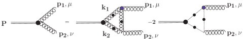
Figure 1: Diagrammatic representation of the Bethe-Salpeter equation for gluon (wiggly lines) bound states (double line). The irreducible one-particle vertices and the full propagators are represented and marked by filled blobs.

II.1 BS amplitude for Pseudoscalar glueballs

The BS amplitude of a colorless pure glueball with total spin and parity $J^{\pi}$ and total momentum $P$ is defined in the standard way,

$$A^{\mu\nu}(x_{1},x_{2})=\left\langle 0\left|T\left[\hat{A}^{\mu}(x_{1})\hat{A}^{\nu}(x_{2})\right]\right|J^{\pi},P\right\rangle,$$ (1)

where, for brevity, the color indices of the gluon field operators $\hat{A}_{\mu,\nu}(x)$ are suppressed. Usually one considers the Fourier transform $A^{\mu\nu}(p_{1},p_{2})$ of the amplitude (1), which due to translation invariance, depends on the relative momentum $p=(p_{1}-p_{2})/2$ and the total momentum, $P=(p_{1}+p_{2})$, of the glueball. By definition, the amplitude $A^{\mu\nu}(p_{1},p_{2})$ is transverse

$$p_{1\mu}A^{\mu\nu}(p_{1},p_{2})=A^{\mu\nu}(p_{1},p_{2})p_{2\nu}=0.$$ (2)

Often, instead of the BS amplitude $A^{\mu\nu}(p_{1},p_{2})$ one considers the BS vertex function $G_{\alpha\beta}(p_{1},p_{2})$ defined as

$$A^{\mu\nu}(p_{1},p_{2})=D^{\mu\alpha}(p_{1})G_{\alpha\beta}(p_{1},p_{2})D^{\beta\nu}(p_{2}).$$ (3)

From (2) it follows that the BS vertex $G_{\alpha\beta}(p_{1},p_{2})$ is also transverse

$$p_{1\mu}A^{\mu\nu}(p_{1},p_{2})=p_{1\mu}D^{\mu\alpha}(p_{1})G_{\alpha\beta}(p_{1},p_{2})D^{\beta\nu}(p_{2})=-i\xi\frac{p_{1\alpha}}{p_{1}^{2}}G_{\alpha\beta}(p_{1},p_{2})D^{\beta\nu}(p_{2})=0,$$

$$A^{\mu\nu}(p_{1},p_{2})p_{2\nu}=-i\xi D^{\mu\alpha}(p_{1})G_{\alpha\beta}(p_{1},p_{2})\frac{p_{2\beta}}{p_{2}^{2}}=0,$$ (4)

where $\xi$ is the gauge parameter of the gluon propagator, $D^{\mu\nu}(p)=-i\frac{Z(p)}{p^{2}}\left(g^{\mu\nu}-\frac{p^{\mu}p^{\nu}}{p^{2}}\right)-i\xi\frac{p^{\mu}p^{\nu}}{p^{4}}$, where $Z(p)$ is the corresponding dressing functions. In what follows we work in Landau gauge, $\xi\to 0$. From (4) a useful relation follows:

$$A^{\mu\nu}(p_{1},p_{2})=D^{\mu\alpha}(p_{1})G_{\alpha\beta}(p_{1},p_{2})D^{\beta\nu}(p_{2})=-\frac{Z(p_{1}^{2})Z(p_{2}^{2})}{p_{1}^{2}p_{2}^{2}}G^{\mu\nu}(p_{1},p_{2}).$$ (5)

With these preliminary notations, the BS amplitude and BS vertex for a pseudo-scalar glueball (the first r.h.s. diagram in Fig. 1) read as

$$A_{\mu\nu}(p_{1},p_{2})=D_{\mu\mu_{1}}(p_{1})\left(-N_{c}\int\frac{d^{4}k}{(2\pi)^{4}}\Gamma_{1}^{\mu_{1}\alpha\lambda}(p_{1},k_{1},\kappa)A_{\alpha\beta}(k_{1},k_{2})\Gamma_{2}^{\nu_{1}\beta\lambda_{1}}(p_{2},k_{2},\kappa)D_{\lambda\lambda_{1}}(\kappa)\right)D_{\nu\nu_{1}}(p_{2}),$$

(6)

for the amplitude, and

$$G_{\mu\nu}(p_{1},p_{2})=-\left[\frac{Z_{1}(p_{1})Z_{2}(p_{2})}{p_{1}^{2}p_{2}^{2}}\right]^{-1}A_{\mu\nu}(p_{1},p_{2})=$$

$$=t_{\mu\mu_{1}}(p_{1})\left(-N_{c}\int\frac{d^{4}k}{(2\pi)^{4}}\frac{Z_{1}(k_{1}^{2})Z_{2}(k_{2}^{2})}{k_{1}^{2}k_{2}^{2}}\Gamma_{1}^{\mu_{1}\alpha\lambda}(p_{1},k_{1},\kappa)G_{\alpha\beta}(k_{1},k_{2})\Gamma_{2}^{\nu_{1},\beta\lambda_{1}}(p_{2},k_{2},\kappa)D_{\lambda\lambda_{1}}(\kappa)\right)t_{\nu\nu_{1}}(p_{2}),$$

(7)

for the BS vertex. In the above equations, $\Gamma_{1}^{\mu_{1}\alpha\lambda}(p_{1},k_{1},\kappa)$ and $\Gamma_{2}^{\nu_{1},\beta\lambda_{1}}(p_{2},k_{2},\kappa)$ are the $3g$-vertices corresponding to the first r.h.s. diagram in Fig. 1, and $t_{\mu\nu}(p)\equiv\left(g_{\mu\nu}-\displaystyle\frac{p_{\mu}p_{\nu}}{p^{2}}\right)$ denotes the transverse projection operator. Observe that, due to the presence of $t_{\mu\nu}(p_{1,2})$ both, the BS amplitude (6) and the BS vertex function (7), are manifestly transverse. In principle, these two equations are completely equivalent. The only difference is that in the equation for the BS amplitude the two gluon propagators are outside the loop integral, while for the BS vertex functions the gluon propagators are subjects of a four-dimensional integration. As mentioned above consistency of the approach requires that the gluon propagators in (6)-(7) are solutions of the tDS equation obtained within the same approach as the tBS equation. As a rule, even in the simplest case, the tDS equation is solved numerically. This causes additional difficulties in (6)-(7) when carrying out the angular integrations. However, since in eq. (6) the numerical solutions of the tDS equation are outside the integral, such numerical problems can be essentially minimized. Moreover, employing a specific form of the phenomenological interaction kernel in (6) all angular integrations, over the spacial and hyper angles of the integration momentum $k$, can be performed analytically (see below). This is the reason to consider the BS amplitude rather than the vertex (7).

Prior to proceed with calculations of the amplitude (6) we come back to the solutions of the tDS equations, reported in Ref. EJPPlus , and re-analyse the effective parameters of the model in the context of a simultaneous description of the gluon propagators from tDS and the BS amplitude from tBS equations.

II.2 Coupled Dyson-Schwinger equations for gluons and ghosts

In most approaches, the tDS equation usually is solved numerically by implementing different approximation schemes. The simplest one consists in a replacement of the fully dressed three-gluon and ghost-gluon vertices by their bare values, a procedure known as the Mandelstam approximation CPCMandelstam ; MANDELSTAM_Approx ; PennigtonMandels and the y-max approximation YmaxApprox . In order to simplify the angular integration, in the Mandelstam approximation the gluon-ghost coupling is neglected. In Ref. YmaxApprox the coupling of the gluon to the ghost was considered, however additional simplifications for the gluon, $Z(k^{2})$, and ghost, $G(k^{2})$, dressing functions have been introduced, again to facilitate the angular integrations and the analytical and numerical analysis of the resulting equations. A more rigorous analysis of the tDS equation has been presented in a series of publications (see, e.g. Refs. IRGluonProp_AlkoferSmekal ; FischerPhD ; SmekalAnnPhys ; Fischer_Alkofer_Reinhard and references therein), where much attention has been focused on a detailed investigation of the gluon-gluon and ghost-gluon vertices and on the implementation of the Slavnov-Taylor identities for these vertices. With some additional approximations the infrared behavior of gluon and ghost propagators has been obtained analytically and compared with the available lattice QCD calculations. In Ref. PawlowskyFicher a thorough analysis of the relevance of the Slavnov-Taylor identities, renormalization procedures and divergences in the tDS equation is presented in some detail. Comparison of the numerical calculations for the gluon and ghost dressing functions and running coupling $\alpha_{s}$ with lattice data have been presented as well. Similar calculations together with a comparison with lattice data are presented also in Ref. IRGreen_FewBody2012 (for a more detailed review see Ref. FisherReview and references therein quoted).

In EJPPlus we suggested an approach based on the rainbow approximation to solve the tDS system of equations for gluon and ghost dressing functions. It has been shown that it is possible to establish a set of effective parameters to describe reasonable well the lattice SU(2) data. Also, it has been mentioned that such a set of parameters is not unique; one can find several different sets of parameters which also provide good descriptions of data. Recall that, in case of quarkonia (mesons) the effective rainbow parameters have been fitted also to describe the lowest quark-antiquark bound states (pions) and the quark-antiquark condensate. Contrary to this case, in Ref. EJPPlus the parameters have been adjusted to lattice data solely for the propagator functions without any connection to possible bound states. Here we come back to the tDS equation and re-fit the parameters with the scope of providing simultaneously a good solution for the gluuon and ghost propagators and reasonable results for the ground state of the pseudo-scalar glueballs.

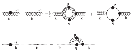
Figure 2: Diagrammatic representation of the employed tDS equations for gluon (top line) and ghost (bottom line) propagators. The internal wiggly and dashed lines denote the full propagators marked by filled blobs. The irreducible one-particle vertices are also denoted by filled blobs. In the gluon tDS equation, terms with four-gluon vertices and quark loops have been dismissed.

II.3 tDS equation within the rainbow approximation

Diagrammatically, the system of coupled tDS equations for the gluon and ghost propagators is presented in Fig. 2. The explicit expressions for these diagrams have been computed within the rainbow approximation and presented in some details in Ref. EJPPlus . Since we are interested in bound states, where the main contribution comes from the infra-red region, particular attention in Ref. EJPPlus has been paid to the conjecture about the behaviour of the gluon dressing function $Z(p^{2})$ and ghost dressing function $G(p^{2})$ at the origin. So, if one adopts finiteness of the ghost dressing and $Z(p^{2})\sim p^{2}$, then a family of the so-called decoupling solutions are generated, cf. PawlowskyFicher . Contrarily, the scaling solutions imply a divergent ghost dressing ($G(0)\to\infty$) and $Z(p^{2})\sim(p^{2})^{\kappa}$ with $0.5<\kappa<1$ at the origin SmekalAnnPhys . A detailed discussion on the scaling and decoupling solutions can be found in Ref. Huber . In principle both, decoupling and scaling solutions are admitted by the existing lattice QCD results. Nonetheless, there are some indications  Bowman ; Muller about regularity at $p^{2}=0$. In the present paper we consider the tDS equations corresponding to the decoupling solutions. Recall that the rainbow approximation consists in replacing the dressed vertices together with the dressed exchanging propagators by their bare quantities augmented by some effective form factors

$$\!\!\!\!\!\!\!\!\!\!\!\!\!\!\left[\frac{g^{2}}{4\pi}\Gamma_{\mu_{1}\alpha\lambda}^{(0)}(p_{1},k_{1},\kappa)D^{\lambda\lambda_{1}}(\kappa^{2})\Gamma_{\nu_{1}\beta\lambda_{1}}(p_{2},k_{2},\kappa)\right]=\Gamma_{\mu_{1}\alpha\lambda}^{(0)}(p_{1},k_{1},\kappa)t^{\lambda\lambda_{1}}(\kappa)\Gamma_{\nu_{1}\beta\lambda_{1}}^{(0)}(p_{2},k_{2},\kappa)F^{eff}_{1}(p^{2}),$$ (8)

$$\!\!\!\!\!\!\!\!\!\!\!\!\!\!\left[\frac{g^{2}}{4\pi}D_{G}(p^{2})\Gamma_{\nu}(p)\right]=\Gamma_{\nu}^{(0)}(p)F^{eff}_{2}(p^{2}),$$ (9)

$$\!\!\!\!\!\!\!\!\!\!\!\!\!\!\left[\frac{g^{2}}{4\pi}\Gamma_{\mu}^{(0)}(q)D^{\mu\nu}(p^{2})\Gamma_{\nu}(k,q,p)\right]=\Gamma_{\mu}^{(0)}(q)t^{\mu\nu}(p)\Gamma_{\nu}^{(0)}(k)F^{eff}_{3}(p^{2}),$$ (10)

where the above three terms correspond to three loop diagrams in Fig. 2. Since we are interested bound states, i.e. mostly in the range of internal momenta corresponding to the infra-red region, in the present paper we use for $F^{eff}(p^{2})$ the Gaussian form with two terms for $F^{eff}_{1,2}(p^{2})$ and one term for $F^{eff}_{3}(p^{2})$ as in ourFB ; dorkinBSmesons ; OurAnalytical ; EJPPlus . This is quite sufficient to obtain a reliable solution of the system of tDS equations. Such a Gaussian representation of the interaction kernels has been widely employed previously for quarkonia and is known as the AWW kernel Alkofer . Explicitly, in Euclidean space the effective form factors are chosen as

$$F^{eff}_{1}(p^{2})=D_{11}\frac{\tilde{p}^{2}}{\omega_{11}^{6}}\exp{\left(-\tilde{p}^{2}/\omega_{11}^{2}\right)}+D_{12}\frac{\tilde{p}^{2}}{\omega_{12}^{6}}\exp{\left(-\tilde{p}^{2}/\omega_{12}^{2}\right)},$$ (11)

$$F^{eff}_{2}(p^{2})=\frac{D_{2}}{\omega_{2}^{4}}\exp{\left(-\tilde{p}^{2}/\omega_{2}^{2}\right)},$$ (12)

$$F^{eff}_{3}(p^{2})=D_{21}\frac{\tilde{p}^{2}}{\omega_{21}^{6}}\exp{\left(-\tilde{p}^{2}/\omega_{21}^{2}\right)}+D_{22}\frac{\tilde{p}^{2}}{\omega_{22}^{6}}\exp{\left(-\tilde{p}^{2}/\omega_{22}^{2}\right)},$$ (13)

where, from now and throughout the rest of the paper, $\tilde{p}$ denotes the modulus of the four vector $p$ in Euclidean space. With such a choice of the effective interaction, the angular integration can be carried out analytically EJPPlus leaving h a system of one-dimensional integral equations in Euclidean space. We found that for the set of parameters $\omega_{11}=1.095$ GeV, $\omega_{12}=2.15$ GeV, $D_{11}=0.465\ {\rm GeV}^{2}$, $D_{12}=0.116\ {\rm GeV}^{2}$ for the 3-gluon loop and $\omega_{21}=2/3\ \omega_{11}$ , $\omega_{22}=\omega_{12}$ , $D_{21}=0.4\pi\ {\rm GeV}^{2}$, $D_{22}=0.1\pi\ {\rm GeV}^{2}$ for the gluon-ghost loop and $\omega_{2}=0.58$ GeV and $D_{2}=7.7\ {\rm GeV}^{2}$ for the ghost loop, the solution the tDSE describes quite well the lattice SU(2) results. Figures 3,4 demonstrate the obtained solution for the ghost and gluon dressing functions and for the gluon propagator, respectively, in comparison to the lattice results BornyakovLattice ; GhostLatticeMishaPRD .

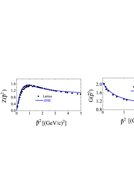
Figure 3: (Color online) Solution of the tDS equations (solid lines) in comparison with lattice SU(2) calculations BornyakovLattice ; GhostLatticeMishaPRD (filled circles). Left panel: gluon dressing function, right panel: ghost dressing function.

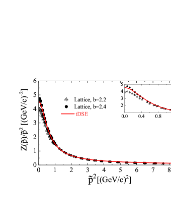
Figure 4: (Color online) Solution of the tDS equations (solid lines) for the gluon propagator in comparison with lattice SU(2) data BornyakovLattice ; GhostLatticeMishaPRD (filled circles and symbols). The inset is a zoom into the infra-red region.

The obtained good description of the lattice data justifies our use of the tDSE to obtain the gluon propagators in the complex plane and the employment of the above effective parameters in solving the tBS equation for glueballs.

III Rainbow approximation of the tBS amplitude

By the definition, the BS pseudoscalar amplitude (1) and the BS pseudoscalar vertex (3) are antisymmetric w.r.t $p_{1}\leftrightarrows p_{2}$ and $(\mu,\nu)\leftrightarrows(\nu,\mu)$ (for a thorough analysis of two-photon/gluon states, see Ref. landau ). The most general form of such pseudo-scalar amplitudes can be written in the form

$$A^{\mu\nu}(p_{1},p_{2})=F(p_{1}^{2},p_{2}^{2},(p_{1}\cdot p_{2}))\epsilon^{\mu\nu\alpha\beta}p_{1\alpha}p_{2\beta}\equiv F(p^{2},P^{2},(p\cdot P))\epsilon^{\mu\nu\alpha\beta}p_{\alpha}P_{\beta},$$ (14)

where the scalar functions $F(p^{2},P^{2},(p\cdot P))$, for a given glueball mass $M_{gg}^{2}=P^{2}$, depends solely on the relative momentum $p^{2}$ and the hyper angle, $\cos\xi_{p}$, between $p$ and $P$. Moreover, they are even functions of $\cos\xi_{p}$. To release the tensor structure of the amplitude (14) we multiply it by $\epsilon_{\mu\nu}^{\phantom{\alpha\beta}\rho\sigma}p_{\rho}P_{\sigma}$ and contract all the Lorentz indices. The result is

$$A^{\mu\nu}(p,P)\ \epsilon_{\mu\nu}^{\phantom{\alpha\beta}\rho\sigma}\ p_{\rho}P_{\sigma}=2F(p^{2},M_{gg}^{2},\cos\xi_{p})p_{\rho}P_{\sigma}\left(g^{\alpha\sigma}g^{\beta\rho}-g^{\alpha\rho\beta\sigma}\right)p_{\alpha}P_{\beta}=$$

$$2F(p^{2},M_{gg}^{2},\cos\xi_{p})\left[(p\cdot P)^{2}-p^{2}P^{2}\right].$$ (15)

The explicit expression for the amplitude (15), within the rainbow approximation, is obtained by direct computation of the (first r.h.s.) diagram in Fig. 1. Taking into account the transversality of the amplitude, the free 3-gluon vertices can be written as

$$\Gamma_{1}^{\mu_{1}\alpha\lambda}(p_{1},k_{1},\kappa)=-2g\left[p_{1}^{\lambda}g^{\mu_{1}\alpha}-k_{1}^{\mu_{1}}g^{\alpha\lambda}-p_{1}^{\alpha}g^{\lambda\mu_{1}}\right],$$ (16)

$$\Gamma_{2}^{\nu_{1}\beta\lambda_{1}}(p_{2},k_{2},\kappa)=-2g\left[k_{2}^{\nu_{1}}g^{\beta\lambda_{1}}-p_{2}^{\lambda_{1}}g^{\beta\nu_{1}}+p_{2}^{\beta}g^{\lambda_{1}\nu_{1}}\right].$$ (17)

Further, we contract the Lorentz indices in the amplitude (6) with the bare vertices (16)-(17), and the results are transformed in to Euclidean space, where the rainbow form factors are defined. As a result we are left with a four-dimensional integration $d^{4}k=\tilde{k}^{3}d\tilde{k}\sin^{2}\xi_{k}d\xi_{k}d\Omega_{\bf k}$, where $\xi_{k}$ and $\Omega_{\bf k}$ are the the hyper and spatial angles of the momentum $k$. The scalar function $F(\tilde{p}^{2},M_{gg}^{2},\cos\xi_{p})$ in (14) is then decomposed over a complete set of the Gegenbauer polynomials of the first order $G_{M_{p}}^{(1)}(\cos\xi_{p})$ (the Chebyshev’s polynomials $U_{M_{p}}(\cos\xi_{p})$ of the second kind):

$$F(\tilde{p}^{2},M_{gg}^{2},\cos\xi_{p})\sin^{2}\xi_{p}=\sum\limits_{M_{p}=even}F_{M_{p}}(\tilde{p}^{2},M_{gg}^{2})\sin^{2}\xi_{p}G_{M_{p}}^{(1)}(\cos\xi_{p}),$$ (18)

where the partial amplitudes $F_{M_{p}}(\tilde{p}^{2},M_{gg}^{2})$, for a given glueball mass $M_{gg}$, are functions of only the relative momentum $\tilde{p}^{2}$. Calculations of the (first r.h.s. ) diagram in Fig. 1 within the above definitions and approximations result in

$$F_{M_{p}}(\tilde{p}^{2},M_{gg}^{2}) = \frac{2}{\pi}\frac{1}{M_{gg}^{2}\tilde{p}^{2}}\int\limits_{0}^{\pi}\frac{|Z(\tilde{p}_{1})|^{2}G_{M_{p}}^{(1)}(\cos\xi_{p})}{|\tilde{p}_{1}^{2}|^{2}}d\xi_{p}$$ (19)

$$\times \sum\limits_{M_{k}=even}\int\tilde{k}^{3}d\tilde{k}\sin^{2}\xi_{k}d\xi_{k}d\Omega_{\bf k}F_{M_{k}}(\tilde{k}^{2},M^{2})G_{M_{k}}^{(1)}(\cos\xi_{k})\big{(}\ldots\big{)},$$

where $\tilde{p}_{1}^{2}=\tilde{p}_{2}^{2*}=-M_{gg}^{2}/4+\tilde{p}^{2}+iM_{gg}\tilde{p}\cos\xi_{p}$ is the momentum of one of the constituent gluon in the Euclidean complex plane and the brackets denote symbolically the result of contraction of the Lorentz indices in the expression (6). The color factor $N_{c}=-3$ and the corresponding powers of $(2\pi)^{4}$ from the space volume integration are also included into $\big{(}\ldots\big{)}$. From (6) and (14) one infers that the result of contracting indices is expressed in terms of some powers of four-products $(p\cdot P)^{N}=(iM_{gg}\tilde{p}\cos\xi_{p})^{N}$, $(k\cdot P)^{L}=(iM_{gg}\tilde{k}\cos\xi_{k})^{L}$ and $(p\cdot k)^{\delta}=(\tilde{p}\tilde{k}\cos\xi_{pk})^{\delta}$. In total, in (19) one has a five-dimensional integral. It can be essentially reduced by observing that the spatial dependence $\Omega_{\bf kp}$ of the integrand enters solely via the hyper angle $\cos\xi_{pk}\equiv x_{kp}=\cos\xi_{p}\cos\xi_{k}+\sin\xi_{p}\sin\xi_{k}\cos\theta_{\bf pk}$, where $\theta_{\bf pk}$ is the spatial angle between vectors p and k. There are two sources of the hyper angle $\xi_{pk}$ dependence in (19): i) the scalar product $(p\cdot k)^{\delta}=(\tilde{p}\tilde{k}x_{kp})^{\delta}$ which originates from the contractions of the Lorentz indices and ii) the rainbow form factors $F^{eff}\left(\tilde{p}^{2}\right)$, which enters via the Gaussian exponents, $\exp{\left(-(p-k)^{2}/\omega^{2}\right)}=\exp{\left(-(\tilde{p}^{2}+\tilde{k}^{2})/\omega^{2}\right)}\cdot\exp(\alpha x_{kp}),$ where $\alpha=2\tilde{k}\tilde{p}/\omega^{2}$. As a result, the $x_{kp}$-dependence of the integrand (19) is of the form ”$\exp(\alpha x_{kp})x_{kp}^{\delta}$”, which can further be handled by decomposing it, as above, over the same full set of the Gegenbauer polynomials $G_{M_{v}}^{(1)}(x_{kp})$.

Then the integrated over the spatial angles $d\Omega_{\bf k}$ of the corresponding parts of the amplitude can be written as

$$\int{\rm e}^{\alpha x_{kp}}x_{kp}^{\delta}d\Omega_{\bf k}=8\pi\sum_{M_{v}}\frac{d^{\delta}}{d\alpha^{\delta}}\left[\frac{1}{\alpha}I_{M_{v}+1}(\alpha)\right]G_{M_{v}}^{(1)}(x_{k})G_{M_{v}}^{(1)}(x_{p}),$$ (20)

where $I_{M}(\alpha)$ denotes the Bessel functions of the second kind (for details, see Appendix A). The remaining angular integration over the hyper angle $\cos\xi_{k}\equiv x_{k}$ is of the form

$${\cal K}_{M_{k},M_{v}}^{L}=\int\limits_{-1}^{1}G_{M_{k}}^{(1)}(x_{k})G_{M_{v}}^{(1)}(x_{k})x_{k}^{L}\sqrt{1-x_{k}^{2}}dx_{k},$$ (21)

which can be also presented in a closed analytical form (see Appendix B). In eq. (21), $M_{v}$ comes from decomposition of the rainbow exponent (20), $M_{k}$ from the partial decomposition (18) of the amplitude $F(\tilde{k}^{2},M_{gg}^{2},\cos\xi_{k})$, and the term $x_{k}^{L}$ comes from the scalar product $(k\cdot P)^{L}=(iM_{gg}\tilde{k}\cos\xi_{k})^{L}$ which results from the contraction of the Lorentz indices. Then the r.h.s. of the tBS equation receives the form

$$F_{M_{p}}(\tilde{p}^{2},M^{2})=\frac{2}{\pi}\frac{1}{M_{gg}^{2}\tilde{p}^{2}}\sum\limits_{i=1}^{2}\sum_{M_{k}=0}^{M_{max}}\sum_{M_{v}=0}^{M_{k}+3}$$

$$\int\limits_{0}^{\infty}d\tilde{k}\tilde{k}^{3}\int\limits_{-1}^{1}\frac{|Z(\tilde{p}_{1}^{2})|^{2}G_{M_{p}}^{(1)}(x_{p})G_{M_{v}}^{(1)}(x_{p})}{|\tilde{p}_{1}^{2}|^{2}\sqrt{1-x_{p}^{2}}}dx_{p}\sum_{L,\delta}C_{L,\delta}(\tilde{k},\tilde{p},x_{p}){\cal K}_{M_{k},M_{v}}^{L}{\cal I}_{M_{v}}^{(\delta)}(\alpha_{i})F_{M_{k}}(\tilde{k}^{2},M_{gg}^{2}),$$ (22)

where ${\cal I}_{M_{v}}^{(\delta)}(\alpha_{i})=\displaystyle\frac{d^{\delta}}{d\alpha^{\delta}}\left[\displaystyle\frac{1}{\alpha}I_{M_{v}+1}(\alpha_{i})\right]$ with $\alpha_{i}=2\tilde{p}\tilde{k}/\omega_{i}^{2}$. Note that from a dimension analysis of the expression for the amplitude it follows that $L=0...3$, $\delta=0...(3-L)$. The explicit expressions for the coefficients $C_{L,\delta}(\tilde{k},\tilde{p},x_{p})$ can be obtained by an analytical manipulation package (e.g., Maple or Mathematica). Their explicit expressions are quite cumbersome and are not presented here.

IV Numerical calculations

Expression (22) is the main equation to be solved for the pseudo-scalar pure glueballs. Recall that eq. (22) is written in Euclidean space, where momenta of the constituent glueballs are complex and, consequently, the gluon propagators entering eq. (22) have to be defined in the complex Euclidean plane.

IV.1 Gluon propagator in the complex Euclidean plane

The solution of the tDS equation along the positive real axis of momenta has to be generalized to complex values of $\tilde{p}_{1,2}^{2}$, needed to solve the tBS equation for bound states. Note that the tDS solutions are needed not in the the whole Euclidean complex space, but only in the kinematical domain where the tBS equation is defined. This is a restricted portion of Euclidean space which is determined by the complex momenta of the gluon propagators $\tilde{p}_{1,2}^{2}$. Usually this domain is displayed as the dependence of the imaginary part of the constituent gluon momentum squared, Im $\tilde{p}_{1,2}^{2}$, on its real part, Re $\tilde{p}_{1,2}^{2}$, determined by the tBS equation. In terms of the relative momentum $\tilde{p}$ of the two gluons residing in a glueball, the corresponding dependence is

$$\tilde{p}_{1,2}^{2}=-\displaystyle\frac{M_{gg}^{2}}{4}+\tilde{p}^{2}\pm iM_{gg}\tilde{p}$$ (23)

determining in the Euclidean complex momentum plane a parabola  Im $\tilde{p}^{2}=\pm~{}M_{gg}\sqrt{{\rm Re}\,\tilde{p}^{2}~{}+~{}\frac{M_{gg}^{2}}{4}}$ with vertex at Im $\tilde{p}^{2}=0$ at Re $\tilde{p}^{2}=-M_{gg}^{2}/4$ depending on the glueball mass $M_{gg}$. In the previous analysis dorkinBSmesons ; OurAnalytical of the quark propagators within the rainbow approximation it was found that the corresponding propagator functions may posses pole-like singularities in the left hemisphere of the parabola, Re $\tilde{p}^{2}<0$, which hamper the numerical procedure of solving the tBS equation. Exactly the same situation occurs also for the gluon and ghost dressing functions as rainbow solutions of tDS equations, cf. Ref. EJPPlus . It should be noted that the pole-like singularities of the propagators appear not only because of specific choice of the rainbow kernel. There are also some other considerations, based on studies of the gauge fixing problem, according to which the gluon propagator contains complex conjugate poles in the negative half-plane of squared complex momenta $\tilde{p}_{1,2}^{2}$, not mandatorily related to the rainbow approximation ZwangerANalit ; Stingl ; CucchieriAnalit .

There are several possible procedures (cf. Refs. analiticalFischer ; GluonAnalyticalFisherPRL2012 ) of how to obtain a complex solution of the tDS equations, once the equation has been solved for real and spacelike Euclidean momenta. First, one can use the so-called shell method. This method acknowledges the fact that for fixed external momentum $\tilde{p}^{2}$ the integrand in the tDS equation samples only the mentioned parabolic domain in the complex momentum plane. Therefore, one starts with a sample of external momenta on the boundary of a typical domain very close to the real positive momentum axis. The tDS equations are then solved on this boundary, while the interior points are obtained by interpolation. In the next step, a slightly larger parabolic domain is used, with points in the interior given by the previous solution. This way one extends the solution of the tDS equations step by step further away from the Euclidean result into the whole complex plane. A shortcoming of the method is that there is an accumulation of numerical errors at each step of the calculations.

A second option is to deform the loop integration path itself away from the real positive $\tilde{p}_{1,2}^{2}$ axis OurAnalytical ; MarisComplexDSE . This can be done by deforming the integration contour and solving the integral equation along this new contour. In practice, one changes the integration contour by rotating it in the complex plane, multiplying both the internal and the external variables by a phase factor $e^{i\phi}$. Thus, one gets the complex variables $\tilde{p}=|\tilde{p}|e^{i\phi}$ and $\tilde{k}=|\tilde{k}|e^{i\phi}$ and solves the tDS equation along the rays $\phi=const$. This method works quite well in the first quadrant, $\phi\leq\pi/2$, but fails at $\phi>\pi/2$, see e.g. Refs. OurAnalytical ; dorkinBSmesons . This is because along the rays $\phi=const$ all the values of $|\tilde{p}|$, from $|\tilde{p}|=0$ to $|\tilde{p}|\to\infty$ contribute to the tDS equation, even if one needs the solution only in a restricted area of the parabola Re $\tilde{p}_{1,2}^{2}<0$. Consequently, numerical instabilities are inevitable at $\phi>\pi/2$.

The third method, which we use in this work, consists in finding a solution of the integral equations in a straightforward way from the tDS equation along the real $\tilde{k}_{1,2}$ axis on a complex grid for the external momentum $\tilde{p}_{1,2}$ inside and on the parabola (23). As in the previous case, numerical instabilities in the tDS equation can be caused by oscillations of the exponent ${\rm e}^{-(\tilde{k}_{1,2}-\tilde{p}_{1,2})^{2}/\omega^{2}}$ at large $|\tilde{p}_{1,2}^{2}|$ and/or at large $\tilde{k}_{1,2}^{2}$. However, one can get rid of such a numerical problem by taking into account that the parabola (23) restricts only a small portion of the complex plane at Re $p_{1,2}^{2}<0$, where the numerical problems are minimized. For positive values of Re $\tilde{p}_{1,2}^{2}>0$, where $|\tilde{p}_{1,2}^{2}|$ can be large, i.e. the relative momentum $\tilde{p}$ in (23) can be large, the tBS wave function of a glueball is expected to decrease rapidly with increasing values of its argument $\tilde{p}$, and at $\tilde{p}^{max}\sim 3-4\ {\rm GeV/c}$ to become already sufficiently small. In such manner, one can solve the complex tDS equation at not too large values of $|\tilde{p}_{1,2}^{2}|$, where a reliable calculation of the loop integrals is still possible. Then one takes advantage of the fact that, at larger values of $\tilde{p}$, the highly oscillating integrals, in accordance with the Riemann-Lebesgue lemma, are negligibly small or even vanish at $\tilde{p}\to\infty$. Consequently, one can either completely neglect the contribution to the propagators in this region or use a simple asymptotic parametrization of the real propagators and continue it in the complex plane. In the present paper we use the latter option with explicit parametrizations of lattice data BornyakovLattice to which our effective parameters have been adjusted. Note that attempts to extend the parametrizations of the lattice data from the positive momenta to the left hemisphere of Euclidean plane are inconsistent, since such a procedure can lead to essentially different results differing by orders of magnitudes from each other, see e.g. param . However, for large positive momenta, such an analytical continuation is applicable. In the present paper the complex gluon propagators are found by solving the tDS equations in the the left hemisphere Re $\tilde{p}_{1,2}^{2}<0$ and in a part of the right hemisphere Re $\tilde{p}_{1,2}>0$ determined by the integration momentum $0\leq\tilde{k}\leq(6-7)$ GeV; for the remaining parabolic domain we use the explicit parametrisation of lattice data from Ref. BornyakovLattice .

IV.2 Ingredients for the determinant

Having fixed the complex gluon propagators, the integration over the momentum $\tilde{k}$ is executed by discretizing the integral by a proper choice of the Gaussian mesh. The integration interval $\tilde{k}=[0,\infty]$ is truncated by a sufficiently large value of $\tilde{k}={\cal O}(25)$ GeV. Within this interval, the gluon propagators are determined by solving the tDS equations for $0\leq\tilde{k}<\left(\displaystyle\frac{M_{gg}}{2}+6\right)$ GeV, and by using the parametrization of lattice data BornyakovLattice for larger values of $\tilde{k}$. In such a way, the tBS equation for the amplitude transforms in to a homogeneous system of algebraic equations of the form

$$X=\,SX,$$ (24)

where the vector

$$X^{T}=\left[F_{Mp=0}(\tilde{p}_{1}),F_{Mp=0}(\tilde{p}_{2}),\ldots F_{Mp=0}(\tilde{p}_{N_{G}}),\ldots F_{Mp=M^{max}}(\tilde{p}_{1}),F_{Mp=M^{max}}(\tilde{p}_{2}),\ldots F_{Mp=M^{max}}(\tilde{p}_{N_{G}})\right],$$ (25)

for a given value of $M_{gg}$, represents the sought solution in the form of a group of sets of partial wave components $F_{M_{p}}(\tilde{p}_{i})$, specified on the integration mesh of the order $N_{G}$ and the maximum number $M^{max}$ of the Gegenbauer polynomials used in (18). In our calculations we use $M^{max}=4-5$, i.e. the Gegenbauer polynomials, which must be even functions of their arguments, run from $G_{M_{p}=0}^{(1)}(x_{p})$ to $G_{M_{p}=6,8}^{(1)}(x_{p})$. Actually, we found that already for $M_{p}=6$ the convergence of the solution is rather good. However, the final results are obtained for $M^{max}=5$, i.e. the maximum order of the Gegemnbauer polynomial in (18) is $M_{p}=8$. The resulting matrix $S$ is of dimension $N_{S}\times N_{S}$, where $N_{S}=N_{G}\times M^{max}$. In our calculations we use a Gaussian mesh with $64$ nodes in the left hemisphere of the parabola and $96$ for the rest of the integration domain. In total the Gaussian mesh in our calculations consists of $160$ nodes, so that the dimension of the matrix $S$ is $800\times 800$ which is not too large to obtain reliable numerical results. Since the system (24) is homogeneous, the eigenvalue solution is obtained from the condition $\Delta=\det(S-\mathbb{I})=0$. More details about the numerical algorithms of solving the BS equation can be found elsewhere, cf. Refs. ourCiofi ; dorkinBSmesons ; dorkinBeyer .

V Results

The solutions of the tBS equation (22) or, equivalently the solutions of eq. (24), are sought as zeros of the determinant of the matrix $(S-\mathbb{I})$. We scan the values of $M_{gg}$ from a minimum value $M_{gg}\sim 0.1$ GeV to a maximum value $M_{gg}\sim 4$ GeV with a scanning step of $8-10$ MeV. At each stage we compute the corresponding determinant and look for the change of the sign, which clearly would indicate that in the neighbourhood of this interval the determinant has a zero, i.e. this is the sought interval where the solution of tBSE is located. The matrix elements of $S$ are computed with the same set of effective parameters as used in solving the tDS equations for gluon and ghost propagators and which assures a good description of the lattice data, cf. Figs. 3 and 4. In the decomposition of the amplitude over the Gegenbauer polynomials (18) we take into account up to five terms, i.e. $M_{p}=0,2,4,6$ and $8$. The method converges already for 3-4 terms in (18), however for a more stable results we included also $M_{p}=8$. We found that the first zero of the determinant, i.e. the solution for the pure glueball ground states, corresponds to $M_{gg}=2560$ MeV which is quite close to the predictions by the lattice calculations $M_{gg}^{(0)}=2590\pm 136$ MeV Chen ; Morningstar . Next three zeros have been found to be located at $M_{gg}^{(1)}=2620,M_{gg}^{(2)}=2973$ and $M_{gg}^{(3)}=3130$ MeV, which do not have an analogue with lattice data. The next zero at $M_{gg}^{(4)}=3745$ MeV is quite close to the first excited state predicted by lattice calculations, $M_{gg}^{({\rm 1st.})}=3640\pm 189$ MeV. As an illustration, in Fig. 5 we present the behaviour of the absolute value of the determinant as a function of the mass $M_{gg}$ of two dressed gluons in the interval $M_{gg}=2.4-3.8$ MeV where the zeros of the determinant have been detected, i.e. where the bound states occured.

Figure 5: The absolute value of the determinant of the matrix $(S-\mathbb{I})$ in dependence of the glueball mass $M_{gg}$. The deep minima correspond to pure glueball bound states. Ideally, the minima should be proper zeros, however, the finite numerical resolution prevents this. Since the determinant changes its sign at the minima, we attribute them to zeros.

Thus, we see that the obtained mass spectrum is more rich than the one predicted by lattice calculations . This is not a new results in investigations of the energy/mass spectra within relativistic equations. Usually, the corresponding equations provide much more states than the observed real experimental spectrum. Some solutions are in a sense redundant. It is well known that, for quark-antiquark bound states, the tBS equations posses solutions for some combinations $q\bar{q}$ quarkonia which do not exist in nature. For instance, for the pseudo-scalar $q\bar{q}$ states, the tBS approach exhibits solutions for $s\bar{s}$, $c\bar{s}$ etc. dorkinBSmesons which are not detected experimentally. On the other side, the mass spectrum of identified mesons is reproduced within tBS approach with a very good accuracy HilgerQuarkonia , i.e. the real meson spectrum is entirely contained in the spectrum of the numerical solutions of tBS . Yet, nowadays in the literature one starts to discuss the so-called ”abnormal” BS solutions, firstly reported as Wick-Cutkosky amplitudes for the BS equation with interaction kernel mediated by exchange of massless particles karmanov . It is also found that in case of massive exchanging particles some solutions of the (very simplified) BS equations disappear in the non-relativistic limit for the speed of light $c\to\infty$, i.e., presumably such abnormal states cannot be observed experimentally karmanov .

It should be noted furthermore that the lowest lying glueball states have been considered, in a consistent manner, in Ref. glueBS where a Dyson-Schwinger-Bethe-Salpeter approach has been employed. As in the present paper, the gluon propagators entering the tBS scheme have been taken as solutions of the previously solved tDS approach PawlowskyFicher ; GluonAnalyticalFisherPRL2012 and generalized to the complex Euclidean plane. Particular attention in  PawlowskyFicher ; GluonAnalyticalFisherPRL2012 was paid to parametrizations of the three-gluon vertex and the ghost-gluon vertex to satisfy the Slavnov-Taylor identity. The obtained results show a good agreement of the calculated scalar ($0^{++}$) glueball mass ($M_{gg}=1.64\ {\rm GeV}$) with the lattice data ($M_{lat.}=(1.73\pm 0.094)\ {\rm GeV}$), while the computed mass of the pseudo-scalar ($0^{-+}$) glueball ($M_{gg}=4.53\ {\rm GeV}$) is almost twice larger than the lattice predictions ($M_{lat.}=(2.590\pm 0.136)\ {\rm GeV}$). Also, the pseudo-scalar glueballs have been recently considered within the rainbow approximation of the tBS equation in Ref. roberts20New , where the dependence of the glueball mass on the effective slope parameters has been investigated. However, the relevance of the effective rainbow parameters to the gluon and ghost propagators, as well as to the lattice results, has not been discussed.

Having found the values of masses of dressed pure two-gluon states which assure the compatibility of the system (24), one can straight forwardly find the partial BS amplitudes (25). Since the tBS equation is a homogeneous equation, the amplitude can be found up to an arbitrary constant. We solved the system (24) and normalized the partial amplitudes to the maximum value of the first term, $F_{0}(\tilde{p}^{2},M_{gg}^{2})$, which occurs at $\tilde{p}^{2}\sim 1.57\ {\rm GeV}^{2}$. It turns out that in the region of the maximum the first two amplitudes, $F_{0}(\tilde{p}^{2},M_{gg}^{2})$ and $F_{2}(\tilde{p}^{2},M_{gg}^{2})$, are basically of the same magnitude, while the subsequent terms $F_{4}(\tilde{p}^{2},M_{gg}^{2})$, $F_{6}(\tilde{p}^{2},M_{gg}^{2})$ and $F_{8}(\tilde{p}^{2},M_{gg}^{2})$ are essentially smaller, each being smaller than its previous neighbour by a factor $\sim 3$. For instance, at $\tilde{p}^{2}\simeq 6.5\ {\rm GeV}^{2}$ the amplitudes $F_{8}(\tilde{p}^{2},M_{gg}^{2})$ is by more than two order of magnitudes smaller than $F_{0}(\tilde{p}^{2},M_{gg}^{2})$. Also, the amplitudes $F_{0}(\tilde{p}^{2},M_{gg}^{2})$ and $F_{4}(\tilde{p}^{2},M_{gg}^{2})$ are positive in the whole kinematical range, the amplitude $F_{2}(\tilde{p}^{2},M_{gg}^{2})$ is negative everywhere, while the other amplitudes are not of a definite sign. As an illustration of the behaviour of the partial amplitudes, in Fig. 6 we present the main two amplitudes, $F_{0}(\tilde{p}^{2},M_{gg}^{2})$ and $\left|F_{2}(\tilde{p}^{2},M_{gg}^{2})\right|$, as functions of the Euclidean relative momentum $\tilde{p}^{2}$. It is seen that both amplitudes are mainly located around their maximum at $\tilde{p}^{2}\simeq 1.57\ {\rm GeV}^{2}$ sharply decreasing away from the maximum location. Such a $\delta$-function like behaviour is observed for the remaining $F_{4}(\tilde{p}^{2},M_{gg}^{2})$ - $F_{8}(\tilde{p}^{2},M_{gg}^{2})$ partial amplitudes as well. The behavior of the partial amplitudes of the exited stats are basically identical to the ones for the ground state, except that the maximum is shifted towards larger $\tilde{p}^{2}$. Similar qualitative behaviour of the zero’s Chebyshev mode has been recently reported in Ref. roberts20New .

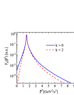
Figure 6: The first two partial amplitudes (Chebyshev’s modes), eq. (18), as functions of the Euclidean momentum $\tilde{p}^{2}$. The presented amplitudes correspond to the BS amplitude for the pseudo-scalar glueball ground state $M_{gg}=2560$ MeV.

VI Summary

In summary, we present a rainbow approximation to the Dyson-Schwinger-Bethe-Salpeter approach to analyse the spectrum mass of pseudo-scalar glueballs. We argue that it is possible to determine a set of effective parameters which describes fairly well the gluon and ghost propagators from the truncated Dyson-Schwinger equation in comparison to the lattice results. The same set of parameters provides the solutions of the Bethe-Salpeter equation for the mass spectrum of the pseudo-scalar glueballs. It is shown that the obtained mass spectrum includes the ground and first excited states predicted by lattice calculations. Besides, in the interval $M_{gg}=2.5-4$ GeV there are more states then predicted by lattice calculations. This is usual situation when solving the equations, non-relativistically and relativistically, for the bound state energies. Some states could be redundant, other ones can belong to the so-called ”relativistic abnormal” states, which disappear in the non relativistic limit, i.e. cannot be detected experimentally. However, the theoretical description of these abnormal states is not yet firmly settled and we do not discuss it in details here.

Appendix A Partial Decomposition of the rainbow kernel

The spatial dependence of the integrand on $\Omega_{\bf k}$ is contained in the rainbow exponents and in the scalar product $(p\cdot k)^{\delta}=(\tilde{p}\ \tilde{k}\ x_{kp})^{\delta}$,

$$\exp(\alpha x_{kp})x_{kp}^{\delta}=\sum_{M_{v}}W_{M_{v}}^{(\delta)}(\tilde{p},\tilde{k})G_{M_{v}}^{(1)}(x_{kp}),$$ (26)

where $\alpha=2\tilde{k}\tilde{p}/\omega^{2}$. The partial coefficients $W_{M_{v}}^{(\delta)}(\tilde{p},\tilde{k})$ can be computed explicitly as

$$W_{M_{v}}^{(\delta)}(\tilde{p},\tilde{k})=\frac{2}{\pi}\int_{-1}^{1}\sqrt{1-x_{kp}^{2}}\exp(\alpha x_{kp})x_{kp}^{\delta}G_{M_{v}}^{(1)}(x_{kp})dx_{kp}=$$

$$\frac{2}{\pi}\frac{d^{\delta}}{d\alpha^{\delta}}\left[\int_{-1}^{1}\sqrt{1-x_{kp}^{2}}{\rm e}^{\alpha x_{kp}}G_{M_{v}}^{(1)}(x_{kp})\right]dx_{kp}=2(M_{v}+1)\frac{d^{\delta}}{d\alpha^{\delta}}\left[\frac{1}{\alpha}I_{M_{v}+1}(\alpha)\right],$$ (27)

where $I_{M_{v}+1}(\alpha)$ are the modified Bessel functions of second kind (of the imaginary argument) yielding

$${\rm e}^{\alpha x_{kp}}x_{kp}^{\delta}=2\sum_{M_{v}}(M_{v}+1)\frac{d^{\delta}}{d\alpha^{\delta}}\left[\frac{1}{\alpha}I_{M_{v}+1}(\alpha)\right]G_{M_{v}}^{(1)}(x_{kp}).$$ (28)

The dependence on the spatial angles of the vectors $\bf p$ and ${\bf k}$ enters via $G_{M_{v}}^{(1)}(x_{kp}\equiv\cos\xi_{kp})$, where $\cos\xi_{kp}=\cos\xi_{p}\cos\xi_{k}+\sin\xi_{p}\sin\xi_{k}\cos\theta_{\bf kp}$. Explicitly, such a dependence can be written by using an addition theorem for Gegenbauer polynomials

$$G_{M_{v}}^{(1)}(x)=\frac{2\pi^{2}}{M_{v}+1}\sum_{l\mu}Z_{M_{v}l\mu}^{*}(p)Z_{M_{v}l\mu}(k)$$ (29)

with $Z_{M_{v}l\mu}(k)=Z_{M_{v}l\mu}(\xi_{k},\theta_{\bf k},\phi_{\bf k})$ as hyper-spherical harmonics, to obtain

$${\rm e}^{\alpha x_{kp}}x_{kp}^{\delta}=4\pi^{2}\sum_{M_{v},l,\mu}\frac{d^{\delta}}{d\alpha^{\delta}}\left[\frac{1}{\alpha}I_{M_{v}+1}(\alpha)\right]Z_{M_{v}l\mu}^{*}(p)Z_{M_{v}l\mu}(k),$$ (30)

where the normalized hyperspherical harmonics are $Z_{M_{v}l\mu}(p)=X_{M_{v}l}(\xi_{p}){\rm Y}_{l\mu}({\bf p})$ with

$$X_{M_{v}l}(\xi_{p})=2^{l}l!\sqrt{\frac{2}{\pi}}\sqrt{\frac{(M_{v}+1)(M_{v}-l)!}{(M_{v}+l+1)!}}\sin^{l}\xi_{p}G_{M_{v}-l}^{l+1}(\cos\xi_{p}).$$ (31)

At a first glance, equations (26)-(31) seemingly even complicate the integration. However, by observing that the dependence of the integrand in (6) on the spatial angles $\Omega_{\bf k}$ is only through the interaction kernel and trough $x_{kp}^{\delta}$, eq. (30), i.e. only trough the spacial harmonics ${\rm Y}_{l\mu}({\bf k})$, the integration over $d\Omega_{\bf k}$ is trivial and eventually we have

$$\int{\rm e}^{\alpha x_{kp}}x_{kp}^{\delta}d\Omega_{\bf k}=8\pi\sum_{M_{v}}\frac{d^{\delta}}{d\alpha^{\delta}}\left[\frac{1}{\alpha}I_{M_{v}+1}(\alpha)\right]G_{M_{v}}^{(1)}(x_{k})G_{M_{v}}^{(1)}(x_{p}).$$ (32)

Appendix B Integrations over $x_{k}$

Hereinbelow we present some details of integrations over the hyper angle $x_{k}$ and the resulting explicit expressions of selection rules. The corresponding angular integral is of the form

$${\cal K}_{M_{v},M_{k}}^{L}=\int\limits_{-1}^{1}\sqrt{1-x_{k}^{2}}x_{k}^{L}G_{M_{k}}^{(1)}(x)G_{M_{v}}^{(1)}(x_{k})dx_{k}.$$ (33)

Due to parity restrictions, the partial amplitudes $F_{M_{k}}$ contain only even values of the Gegenbauer polynomials, i.e. $\ M_{k}=[0,2,4,..M^{max}]$, where $M^{max}$ is the maximum number of polynomials taken into account in concrete calculations. The Gegenbauers $G_{M_{v}}^{(1)}(x_{k})$ which come from the interaction kernel (32) may contain both, even and odd values of $M_{v}$, and formally the summation is extended to infinite, $M_{v}=[0..\infty]$. However, not all values in this interval contribute to (33). The symmetrical limits of integration restrict the Gegenbauer polynomials in (33) to obey the condition ($L+M_{k}+M_{v}$)=even. Other restrictions originate from the explicit expression of the integral, see below. From a standard math handbook one infers that

$$\int\limits_{-1}^{1}\sqrt{1-x^{2}}x^{L}G_{M_{k}}^{(\lambda)}(x)G_{M_{v}}^{(\lambda)}(x)dx=2^{M_{k}+M_{v}}\frac{(2\lambda)_{M_{k}}(2\lambda)_{M_{v}}L!}{m_{k}!M_{v}!(L+M_{k}+M_{v})!}\left(\frac{L-M_{k}-M_{v}}{2}+1\right)_{M_{k}+M_{v}}$$

$$\times B\left(\lambda+\frac{1}{2},\frac{L+M_{k}+M_{v}+1}{2}\right)\!\!\phantom{1}_{3}F_{2}\left(-M_{k},-M_{v},1;2\lambda,\frac{L-M_{k}-M_{v}}{2}+1;1\right),$$ (34)

where $\!\!\phantom{1}{}_{3}F_{2}$ is the generalized hypergeometric function and $(a)_{k}=a(a+1)(a+2)\ldots(a+k-1)$ (with $a_{0}=1$) is the known Pochhammer symbol and $B(x,y)=\displaystyle\frac{\Gamma(x)\Gamma(y)}{\Gamma(x+1)}$ and $\Gamma(x)$ are the familiar Euler $\beta-$ and $\Gamma-$ functions, respectively. Despite the integral (34) is finite, at some values of $L,M_{k}$ and $M_{v}$ the product of the Pochhammer symbol and hypergeometric function can be of the type $0\cdot\infty$, which implies that Eq. (34) cannot be implemented directly in to numerical calculations. One needs to handle zeros and singularities manually. We use the obvious properties

$$(-m)_{k}=(-1)^{k}\frac{m!}{(m-k)!};\qquad(a)_{k}=\frac{\Gamma(a+k)}{\Gamma(a)}$$ (35)

to obtain

$$\left(\frac{L-M_{k}-M_{v}}{2}+1\right)_{M_{k}+M_{v}}=\frac{\kappa!}{\kappa_{1}!};$$ (36)

$$B\left(\frac{3}{2},\frac{L+M_{k}+M_{v}+1}{2}\right)=\frac{\pi}{2^{\kappa+1}}\frac{(2\kappa)!!}{(\kappa+1)!};$$ (37)

$$\!\!\phantom{1}{}_{3}F_{2}\left(-M_{k},-M_{v},1;2,\frac{L-M_{k}-M_{v}}{2}+1;1\right)=\sum_{k=0}^{\infty}\frac{1}{(k+1)!}\frac{M_{k}!M_{v}!}{(M_{k}-k)!(M_{v}-k)!}\frac{\kappa_{1}!}{(\kappa_{1}+k)!},$$

where, for brevity, we introduce the shorthand notation $\kappa=\displaystyle\frac{L+M_{k}+M_{v}}{2}$, $\kappa_{1}=\displaystyle\frac{L-M_{k}-M_{v}}{2}$.

With this notation, the integral (34) reads

$$\int\limits_{-1}^{1}\sqrt{1-x^{2}}x^{L}G_{M_{k}}^{(1)}(x)G_{M_{v}}^{(1)}(x)dx=\pi\frac{2^{M_{k}+M_{v}-\kappa-1}(M_{k}+1)!(M_{v}+1)!L!}{(\kappa+1)(2\kappa)!!}\times$$

$$\sum_{k=0}^{\infty}\frac{1}{(k+1)!(M_{k}-k)!(M_{v}-k)!(\kappa_{1}+k)!}.$$ (39)

In eq. (39) the summation is restricted by those values of $k$ which ensure non-negative factorials, i.e. in the above sum $k\leq M_{k}$ and $k\leq M_{v}$ and $(M_{k}+M_{v}-L+2k)\geq 0$. Together with the condition $(L+M_{k}+M_{v})$-even, these restrictions form the selecting rules for the integral (33). Actually, in practice the summation in (39) consists only of one, or maximum two terms. Consequently, the integrals (33) turn out to be extremely simple being expressed in form of the fractional parts of $\pi$. For instance, the value L=0 results in the orthogonal condition for the Gegenbauer polynomials i.e. ${\cal K}_{M_{k},M_{v}}^{L=0}=\displaystyle\frac{\pi}{2}\delta_{M_{k},M_{v}}$. For $L=1$ one has $M_{v}=1,3,5,7$ and for even $M_{k}=0,2,4,6,8$ the integral (33) is always $\pi/4$, etc.

References

- (1) H. Fritzsch and P. Minkowski, Nuovo Cim. A30, 393 (1975).
- (2) R. L. Jaffe and K. Johnson, Phys. Lett. B 60, 201 (1976).
- (3) U. Wiedner, Prog. Part. Nucl. Phys. 66, 477 (2011).
- (4) S. Jia et al. (The Belle Collaboration), Phys. Rev. D 95, 012001 (2017).
- (5) D. Robson, Z. Phys. C 3 , 199 (1980).
- (6) N. Isgur and J. E. Paton, A Flux Tube Model for Hadrons in QCD, Phys. Rev. D 31, 2910 (1985).
- (7) C. E. Carlson, T. H. Hansson, and C. Peterson, The Glueball Spectrum in the Bag Model and in Lattice Gauge Theories, Phys. Rev. D 30 , 1594 (1984).
- (8) M. S. Chanowitz and S. R. Sharpe, Hybrids: Mixed States of Quarks and Gluons, Nucl. Phys. B 222, 211 (1983) [Erratum Nucl. Phys. B 228, 588 (1983)].
- (9) J. M. Cornwall and A. Soni, Phys. Lett. B 120, 431 (1983).
- (10) Y. M. Cho, X. Y. Pham, P. Zhang, J. J. Xie and L. P. Zou, Phys. Rev. D 91, 114020 (2015).
- (11) N. Boulanger, F. Buisseret, V. Mathieu, and C. Semay, Eur. Phys. J. A 38, 317 (2008).
- (12) J. Leutgeb and A. Rebhan, Phys. Rev. D 101, 014006 (2020).
- (13) L. Bellantuono, P. Colangelo, and F. Giannuzzi, Holographic Oddballs, JHEP 10, 137 (2015).
- (14) Y. Chen and M. Huang, Two-gluon and trigluon, glueballs from dynamical holography QCD, Chin. Phys. C 40, 123101 (2016).
- (15) F. Brunner and A. Rebhan, Holographic QCD predictions for production and decay of pseudoscalar glueballs, Phys. Lett. B 770, 124 (2017).
- (16) M. A. Shifman, A. I. Vainshtein, and V. I. Zakharov, QCD and Resonance Physics. Theoretical Foundations, Nucl. Phys. B 147, 385 (1979).
- (17) E. V. Shuryak, The Role of Instantons in Quantum Chromodynamics. 2. Hadronic Structure, Nucl. Phys. B203, 116 (1982).
- (18) A. Pimikov, H. J. Lee, N. Kochelev, P. Zhang and V. Khandramai, Phys. Rev. D 96, 114024 (2017).
- (19) A. Pimikov, H. J. Lee and N. Kochelev, Phys. Rev. Lett. 119,079101 (2017).
- (20) A. Pimikov, H. J. Lee, N. Kochelev and P. Zhang, Phys. Rev. D 95, 071501 (2017).
- (21) M. Albanese et al. [Ape Collaboration], Phys. Lett. B 197, 400 (1987).
- (22) Y. Chen, A. Alexandru, S. Dong, T. Draper, I. Horvath et al., Phys. Rev. D 73, 014516 (2006).
- (23) C. J. Morningstar and M. J. Peardon, Phys. Rev. D 60, 034509 (1999).
- (24) G. Gabadadze, Phys. Rev. D 58, 055003 (1998).
- (25) W. Ochs, J. Phys. G 40, 043001 (2013).
- (26) H. Noshad, S. M. Zebarjad and S. Zarepour, Nucl. Phys. B 934, 408 (2018).
- (27) H. Sanchis-Alepuz, C. S. Fischer, C. Kellermann and L. von Smekal, Phys. Rev. D 92, 034001 (2015).
- (28) J. Meyers and E. S. Swanson, Phys. Rev. D 87, 036009 (2013).
- (29) P. Maris and C. D. Roberts, Phys. Rev. C 56, 3369 (1997).
- (30) S. M. Dorkin, T. Hilger, L. P. Kaptari and B. Kämpfer, Few Body Syst. 49, 247 (2011).
- (31) P. Maris and C.D. Roberts, Int. J. Mod. Phys. E 12, 297 (2003).
- (32) R. Alkofer, P. Watson and H. Weigel, Phys. Rev. D 65, 094026 (2002).
- (33) C. S. Fischer, P. Watson and W. Cassing, Phys. Rev. D 72, 094025 (2005).
- (34) M. R. Frank and C. D. Roberts, Phys. Rev. C 53, 390 (1996).
- (35) S.M. Dorkin, L.P. Kaptar and B. Kämpfer, Phys. Rev. C 91, 055201 (2015).
- (36) S.M. Dorkin, L.P. Kaptari, T. Hilger and B. Kampfer, Phys. Rev. C 89, 034005 (2014).
- (37) V.B. Berestetskii, E.V. Lifshitz and L.P. Pitaevskii, ”Qunatum Electrodynamics”, p. 29, Pergamon Press, 1982.
- (38) L.P. Kaptari, B. Kämpfer and Pengming Zhang, Eur. Phys. J. Plus 134 (2019) 383.
- (39) A. Hauck, L. von Smekal and R. Alkofer, Comput. Phys. Commun. 112, 149 (1998).
- (40) S. Mandelstam, Phys. Rev. D 20, 3223 (1979).
- (41) K. Buttner and M.R. Pennington, Phys. Rev. D 52, 5220 (1995).
- (42) D. Atkinson and J. C. R. Bloch, Phys. Rev. D 58, 094036 (1998).
- (43) L. von Smekal, A. Hauck and R. Alkofer, Phys. Rev. Lett. 79, 3591 (1997).
- (44) C. S. Fischer, e-Print: hep-ph/0304233 (PhD-thesis, Univ. of Tübingen. Nov 2002).
- (45) L. von Smekal, A. Hauck and R. Alkofer, Ann. Phys. 267, 1 (1998), Erratum: Ann. Phys. 269, 282 (1998).
- (46) C. S. Fischer, R. Alkofer and H. Reinhardt, Phys. Rev. D 65, 094008 (2002).
- (47) C. S. Fischer, A. Maas and J. M. Pawlowski, Ann. Phys. 324, 2408 (2009).
- (48) Ph. Boucaud, J. P. Leroy, A. Le Yaouanc, J. Micheli, O. Pene and J. Rodriguez-Quintero, Few-Body Syst. 53, 387 (2012).
- (49) C. S. Fischer, J. Phys. G 32, R253 (2006).
- (50) P. O. Bowman, U. M. Heller, D. B. Leinweber, M. B. Parappilly, A. Sternbeck, L. von Smekal, A. G. Williams and J. Zhang, Phys. Rev. D 76, 094505 (2007).
- (51) A. Stemrnbeck, M. Müller-Preussker, Phys. Lett. B 276, 396 (2013).
- (52) M. Huber, arXiv:2003.13703 [hep-ph]
- (53) V. G. Bornyakov, V. K. Mitrjushkin and M. Müller-Preussker, Phys. Rev. D81, 054503 (2010).
- (54) V. G. Bornyakov, E.-M. Ilgenfritz, C. Litwinski, M. Müller-Preussker and V. K. Mitrjushkin, Phys. Rev. D 92, 074505 (2015).
- (55) D. Zwanziger, Nucl. Phys. B 323, 513 (1989).
- (56) M. Stingl, Phys. Rev. D 34, 3863 (1986); [Erratum ibid. D 36, 651 (1987)].
- (57) A. Cucchieri, D. Dudal, T. Mendes and N. Vandersickel, Phys. Rev. D 85, 094513 (2012).
- (58) S. Strauss, C. S. Fischer and C. Kellermann, Prog. Part. Nucl. Phys. 67, 239 (2012).
- (59) S. Strauss, C. S. Fischer and C. Kellermann, Phys. Rev. Lett. 109, 252001 (2012).
- (60) P. Maris, Phys. Rev. D 52, 6087 (1995).
- (61) J. Meyers and E. S. Swanson, Phys. Rev. D 87, 036009 (2013) .
- (62) S.M. Dorkin, M. Beyer, S.S. Semikh and L.P. Kaptari, Few Body Syst. 42, 1 (2008).
- (63) S.M. Dorkin, L.P. Kaptari, C. Ciofi degli Atti and B. Kämpfer, Few Body Syst. 49, 233 (2011).
- (64) T. Hilger, M. Gomez-Rocha and A. Krassnigg, Eur. Phys. J. C 77 (2017) 625.
-
(65)
V.A. Karmanov, J. Carbonell and H. Sazdjian,
EPJ Web Conf. 204, 01014 (2019) ;
V.A. Karmanov, J. Carbonell and H. Sazdjian,
e-Print: arXiv:1903.02892;
V.A. Karmanov, J. Carbonell and H. Sazdjian,
e-Print: arXiv:2001.00401. - (66) E. V. Souza, M. N. Ferreira, A. C. Aguilar, J. Papavassiliou, C. D. Roberts and S.-S. Xu, Eur. Phys. J. A56 (2020) 25.