Estimating state occupation and transition probabilities in non-Markov multi-state models subject to both random left-truncation and right-censoring

Abstract

The Aalen-Johansen estimator generalizes the Kaplan-Meier estimator for independently left-truncated and right-censored survival data to estimating the transition probability matrix of a time-inhomogeneous Markov model with finite state space. Such multi-state models have a wide range of applications for modelling complex courses of a disease over the course of time, but the Markov assumption may often be in doubt. If censoring is entirely unrelated to the multi-state data, it has been noted that the Aalen-Johansen estimator, standardized by the initial empirical distribution of the multi-state model, still consistently estimates the state occupation probabilities. Recently, this result has been extended to transition probabilities using landmarking, which is, inter alia, useful for dynamic prediction. We complement these results in three ways. Firstly, delayed study entry is a common phenomenon in observational studies, and we extend the earlier results to multi-state data also subject to left-truncation. Secondly, we present a rigorous proof of consistency of the Aalen-Johansen estimator for state occupation probabilities, on which also correctness of the landmarking approach hinges, correcting, simplifying and extending the earlier result. Thirdly, our rigorous proof motivates wild bootstrap resampling. Our developments for left-truncation are motivated by a prospective observational study on the occurrence and the impact of a multi-resistant infectious organism in patients undergoing surgery. Both the real data example and simulation studies are presented. Studying wild bootstrap is motivated by the fact that, unlike drawing with replacement from the data, it is desirable to have a technique that works both with non-Markov models subject to random left-truncation and right-censoring and with Markov models where left-truncation and right-censoring need not be entirely random. The latter is illustrated for event-driven trials.

Keywords — Nelson-Aalen estimator, Wild bootstrap, Hospital epidemiology, Partly conditional transition rate, Methicillin-resistant staphylococcus aureus

1 Introduction

Aalen and Johansen (1978) developed an estimator of the transition probability matrix of a non-homogeneous Markov multi-state model for independently left-truncated and right-censored data. These models are useful for studying complex courses of a disease over the course of time and applications in medical research include oncology (Schmoor et al., 2013), cardiology (Gasperoni et al., 2017), Gastroenterology (Jepsen et al., 2015), orthopaedics (Gillam et al., 2012) or hospital epidemiology (Munoz-Price et al., 2016). However, the Markov assumption may regularly be in doubt in applications. Our motivating data example (De Angelis et al., 2011) investigated the occurrence and the impact of Methicillin-resistant staphylococcus aureus (MRSA) infection in hospital compared to patients only colonized with MRSA, using an illness-death multistate model. Violations of the Markov assumption arise if the time of MRSA infection affects the hazard of end of hospital stay. See also Andersen et al. (Andersen and Keiding, 2002) for a clear practical discussion of a non-Markov multi-state model.

The Markov assumption enters the technical developments in Aalen and Johansen (1978) (see also Andersen et al. (1993)) in that it implies a particularly handy form of the intensities of the counting processes of observed transitions between any two states of the model. Save for the at-risk processes, these intensities are non-random and equal the usual transition hazards. This is in contrast to the non-Markov case where the intensities will also be random through dependence on the past. For instance, in the MRSA data, such a dependence is present if the time of infection affects the end-of-stay hazard of an infected patient.

For non-Markov models and complete observations, Andersen et al. (Andersen et al., 1993, Section IV.4.1.4) showed that the Aalen-Johansen estimator, standardized by the multinomial estimator of the initial distribution of the multi-state model, results in the usual multinomial estimator of the unconditional state occupation probabilities. Later, Datta and Satten (2001) observed that this approach still yields a consistent estimator of the state occupation probabilities based on right-censored observations provided that censoring is entirely random. Recently, Putter and Spitoni (2016) extended this approach to a landmark Aalen-Johansen estimator of the transition probabilities in randomly right-censored non-Markov multi-state models. Their estimator is based on Aalen-Johansen estimates of the state occupation probabilities computed on subsamples of the data. Consistency of the landmark Aalen-Johansen estimator then follows provided that the Aalen-Johansen estimator of the state occupation probabilities is consistent.

However, these findings do not apply to our data example for two reasons: Firstly, right-censoring is not much of an issue in hospital epidemiology, but delayed study entry, i.e., left-truncation may very well be (Beyersmann et al., 2011). Remarkably, left-truncation was already contained in the seminal paper by Kaplan and Meier (1958), see their Section 2. Our example considers a prospective cohort of patients colonized with MRSA. The time scale of interest is time since hospital admission, and patients may have a delayed study entry if a positive laboratory result is only available some time after admission. Left-truncation is a common phenomenon in observational studies (Bluhmki et al., 2017) and an extension of the findings mentioned above would be generally useful.

Secondly, the arguments of Datta and Satten (2001) are compromised by their use of non-random intensities, which do not apply in non-Markov models, see Müller (2015) and Overgaard (2019). This also affects the recent extension of Putter and Spitoni (2016), because their arguments hinge on consistency of state occupation probability estimation in the landmark data sets. The issue is this: Datta and Satten built on the result of Andersen et al. (1993) for complete data. Their idea was to show that the multivariate Nelson-Aalen estimator, of which the Aalen-Johansen estimator is a transformation, consistently estimates the same limit both in the completely observed and in the randomly right-censored case. Consistency of estimating the state occupation probabilities via the Aalen-Johansen estimator then follows from the continuous mapping theorem, although this approach was not taken by Datta and Satten (2001). For the multivariate Nelson-Aalen estimator, Datta and Satten (2001) started with complete data, used martingale methods similar to Aalen and Johansen (1978) for the Markov case and then transferred results to the right-censored case using inverse probability of censoring weights (Horvitz and Thompson, 1952). However, their arguments used intensities that were, save for the at-risk processes, non-random (see their Equation (A.5)), and use of inverse probability of censoring weights makes the arguments unnecessarily complicated. Overgaard (2019) took a different approach and showed the consistency of the Aalen-Johansen estimator for state occupation probabilities based on interval functions without using martingale arguments. Our approach differs from Overgaard’s in that we will use martingale methods, working, however, with the proper intensities. This approach allows to incorporate left-truncation and lends itself to wild bootstrap resampling which we will find preferable to simple drawing with replacement from the data.

The main aim of this paper is to establish consistent estimation of both state occupation and transition probabilities in non-Markov models subject to both random left-truncation and right-censoring. The main technical results are in Section 2. Here, we start by considering the Nelson-Aalen estimator as an estimator of cumulative partly conditional transition rates, which differ from the transition intensities by only conditioning on the immediate past, but not on the entire history. Simulations are in Section 3. Here, we assess the performance of the Aalen-Johansen estimator for the state occupation probabilities and the landmark Aalen-Johansen estimator for the transition probabilities in non-Markov models. Additionally, we report results on two different resampling methods to obtain confidence intervals. Firstly, we profit from the i.i.d. data structure under random left-truncation and right-censoring, which allow us the use of Efron’s bootstrap. Secondly, we exploit our result on the consistency of cumulative transition hazards estimation in non-Markov models to apply the more flexible wild bootstrap resampling technique (Bluhmki et al., 2018). As the wild bootstrap approach does not necessarily require an i.i.d. data structure we evaluate its performance also in a Markov model subject to event-driven type II censoring. An analysis of the MRSA data is in Section 3.4 and a discussion is in Section 4. Proofs are in the appendix; here, we improve on the arguments of Datta and Satten (2001) by working with the proper intensities which, in a non-Markov model, will also be random through dependence on the past (see Equation (6) below). We will directly work with the observed counting processes such that data may also be randomly left-truncated and inverse probability weighting is not needed.

2 Main technical results

Let $(X(t))_{t\geq 0}$ be a stochastic process with state space $\{0,1,\ldots,K\}$. This multi-state process may be non-Markov with a non-degenerate initial distribution. The first aim is to estimate the state occupation probabilities

$$P(X(t)=m),\,m\in\{0,1,\ldots,K\},t\in[0,\tau].$$ (1)

In a second step, we will also estimate transition probabilities

$$P_{lm}(s,t)=P(X(t)=m\,|\,X(s)=l),\,l,m\in\{0,1,\ldots,K\},s\leq t\in[0,\tau],$$ (2)

using an estimator of $P(X(t)=m)$ in a landmark (sub-) data set that accounts for conditioning on $X(s)=l$. Landmarking for such a purpose has been proposed by Allignol et al. (2014a) for the special case of an illness-death model and later, for general multistate models, by Putter and Spitoni (2016). To this end, define the partly conditional $l\to m$ transition rate (Pepe and Cai, 1993)

$$\alpha_{lm}(t)=\lim_{\Delta t\searrow 0}P(X(t+\Delta t)=m\,|\,X(t)=l),\,l,m\in\{0,1,\ldots,K\},l\neq m,$$ (3)

with cumulative quantities $A_{lm}(t)=\int_{0}^{t}\alpha_{lm}(u){\rm\;d}u$.

We assume that observation of $X$ is subject to random left-truncation by $L$ and right-censoring by $C$. Denote the event of study entry, i.e., X reaches an absorbing state after $L$, by $Z$. Given study entry, consider i.i.d. data $(X_{i}(t))_{t\in(L_{i},C_{i}\wedge T_{i}]}$, $i=1,\ldots,n$, of $n$ individuals under study, where $T_{i}$ is  $i$’s time until absorption and $\wedge$ denotes the minimum. Let $\mathcal{G}(t)$ denote the self-exciting filtration of the observed data $(X_{i}(t))_{t\in(L_{i},C_{i}\wedge T_{i}]}$, $i=1,\ldots,n$.

Define the individual counting process

$$N_{i;lm}(t)=\#\mbox{\ of observed $l\to m$ transitions of $i$ in $[0,t]$},$$ (4)

and the individual at-risk process

$$Y_{i;l}(t)={\bf 1}\left(X_{i}(t-)=l,L_{i}<t\leq C_{i}\right)$$ (5)

such that the counting process of observed $l\to m$ transitions is $N_{lm}(t)=\sum_{i=1}^{n}N_{i;lm}(t)$ and the at-risk process for state $l$ is $Y_{l}(t)=\sum_{i=1}^{n}Y_{i;l}(t)$. Also introduce $J_{l}(t)={\bf 1}(Y_{l}(t)>0)$. We assume that the $N_{i;lm}$’s have absolutely continuous compensators with respect to $\mathcal{G}$, such that

$$M_{lm}(t)=N_{lm}(t)-\int_{0}^{t}\sum_{i=1}^{n}Y_{i;l}(u)\cdot\alpha_{i;lm}(u|\mathcal{G}(u-)){\rm\;d}u,$$ (6)

is a mean zero martingale with respect to $\mathcal{G}$. If $(X(t))_{t\geq 0}$ is time-inhomogeneous Markov, the intensity $\alpha_{i;lm}(t|\mathcal{G}(t-))$ will equal $\alpha_{lm}(t)$ from (3), but in general the intensity will be a random quantity through its dependence on the past.

The Nelson-Aalen estimator is

$$\hat{A}_{lm}(t)=\int_{0}^{t}\frac{J_{l}(u)}{Y_{l}(u)}{\rm\;d}N_{lm}(u),$$

and the Aalen-Johansen estimator is, using product integral notation,

$$\mathop{\lower 1.72218pt\hbox{\huge$\mathit{\pi}$}}_{u\in(0,t]}\left(\mathbf{I}+{\rm\;d}\hat{\mathbf{A}}(u)\right),$$ (7)

where $\mathbf{I}$ is the $(K+1)\times(K+1)$ identity matrix. The matrix $\hat{\mathbf{A}}(t)$ has non-diagonal entries $\hat{A}_{lm}(t)$ and diagonal entries are such that the sum of each row equals zero.

The following result is similar to the classical strong consistency theorem of the multivariate Nelson-Aalen estimator for time-inhomogeneous Markov multi-state models (Andersen et al., 1993, Theorem IV.1.1).

Theorem 2.1

Let $t\in[0,\tau]$ and $l,m\in\{0,1,\ldots,K\},l\neq m$. Assume there exists a function $k$, $\int_{0}^{\tau}k(u){\rm\;d}u<\infty$, such that

$$\alpha_{i;lm}(u|\mathcal{G}(u-))\leq k(u)\mbox{\ on $[0,\tau]$ with probability~{}$1$},$$ (8)

for all $i=1,\ldots n$. Furthermore, as $n\to\infty$, assume that

$$\int_{0}^{t}\frac{J_{l}(u)}{Y_{l}(u)}k(u){\rm\;d}u\to 0\mbox{\ in probability},$$ (9)

and

$$\int_{0}^{t}(1-J_{l}(u))k(u){\rm\;d}u\to 0\mbox{\ in probability}.$$ (10)

Then

$$\sup_{u\in[0,t]}\left|\hat{A}_{lm}(u)-A_{lm}(u)\right|\to 0\mbox{\ in probability}.$$ (11)

The proof of Theorem 2.1 in the Appendix uses the proof of Andersen et al. (Andersen et al., 1993, Theorem IV.1.1) as a template, but with the additional difficulty that $\alpha_{i;lm}(t|\mathcal{G}(t-))$, $i=1,\ldots,n$, are random quantities, unequal to $\alpha_{lm}(t)$. However, assuming i.i.d. multi-state trajectories, these random quantities are i.i.d., too, and their average approaches $\alpha_{lm}(t)$.

Before we turn to estimating state occupation probabilities, some remarks on Theorem 2.1 are in place:

1. In the time-inhomogeneous Markov case, the function $k$ can be chosen as

   $$k(t):=\sum_{l,m,l\neq m}\alpha_{lm}(t),$$

   because the transition hazards are assumed to have finite integrals (Andersen et al., 1993, p. 287).

2. In the presence of left-truncation, the convergence in probability statements are w.r.t. the conditional probability measure given study entry $Z$ from which we sample, see, e.g., Example IV.1.7 of Andersen et al. (1993) and the Appendix. Also note that in the absence of left-truncation the main assumption both in our Theorem 2.1 and in the work by Datta and Satten and as compared to the classical result (Andersen et al., 1993, Theorem IV.1.1) on the Nelson-Aalen estimator is that right-censoring is entirely unrelated to the multi-state process.

3. Analogously to the Markov case, a simple condition that implies assumptions (9) and (10) is that the infimum on $[0,\tau]$ of all risk sets $Y_{l}$ converges in probability to infinity. We refer to Andersen et al. (1993) for an in-depth discussion. This assumption may require reconsidering time $0$ in left-truncated studies. E.g., in hospital epidemiology, a natural time origin is hospital admission. Studies with patients who are colonized with a certain infectious organism upon admission will typically include a substantial proportion of patients with colonization status known at time $0$. Other patients will have left-truncated study entries upon arrival of laboratory results (e.g.,  De Angelis et al., 2011). In this setting, we may assume the condition to be fulfilled. However, in studies on pregnancy outcomes the natural time origin is conception, but women do not enter observational cohorts before pregnancy detection (e.g.,  Slama et al., 2014). Time ‘zero’ in the present context should then be chosen as the earliest time point of detecting pregnancies, around six weeks after the beginning of the menstrual cycle, or perhaps even slightly later, say 7 weeks.

4. In general, left-truncated data may contain information on the multi-state trajectory before study entry, but this information is not used here.

Consistent estimation of the state occupation probabilities now follows from Theorem 2.1.

Theorem 2.2

Suppose $\hat{p}(0)=(\hat{p}_{1}(0),\ldots,\hat{p}_{K}(0))$ is a consistent estimator of the initial distribution of the multi-state model,

$$\hat{p}(0)\to\left(P(X(0)=1),\ldots,P(X(0)=K)\right)\mbox{\ in probability as $n\to\infty$},$$ (12)

and define the $1\times K$ row vector

$$\hat{p}(t)=\hat{p}(0)\cdot\mathop{\lower 1.72218pt\hbox{\huge$\mathit{\pi}$}}_{u\in(0,t]}\left(\mathbf{I}+{\rm\;d}\hat{\mathbf{A}}(u)\right).$$ (13)

Then, under the assumptions of Theorem 2.1, we have that

$$\sup_{u\in[0,t]}\left|\hat{p}(u)-\left(P(X(u)=1),\ldots,P(X(u)=K)\right)\right|\to 0\mbox{\ in probability}.$$ (14)

We prove Theorem 2.2 in the Appendix. The key assumption is (12). The choice of $\hat{p}(0)$ is trivial, if there is one common initial state, say state $0$, with $P(X(0)=0)=1$. In the absence of left-truncation, the obvious choice is the multinomial estimate $\hat{p}_{j}(0)=Y_{j}(0+)/n$. With left-truncation, we will have to rely either on assuming one common initial state, or on an educated ‘guess’ $\hat{p}(0)$, perhaps from some other data source, or on the fact that the individuals at risks are a random draw from the underlying population, which leads to using $\hat{p}_{j}(0)=Y_{j}(0+)/(\sum_{l}Y_{l}(0+))$. Interestingly, this difficulty disappears for the landmark estimator that we discuss next, because the landmark data set is constructed such that there is one common state occupied by all individuals at the landmark time.

2.1 The landmark Aalen-Johansen estimator with left-truncation

The landmark Aalen-Johansen estimator of Putter and Spitoni (2016) is based on subsampling as are the estimators of de Uña-Álvarez and Meira-Machado (2015) and Titman (2015). The idea is to select individuals that are under observation in a given state at a given time and estimate the state occupation probabilities within this subset. Predating these contributions is the work by Allignol et al. (2014a) who derived landmarking for this purpose in the special illness-death model without recovery, already allowing, however, for delayed study entry.

To be precise, let

$$N_{lm}^{({\rm LM})}(t)=\sum_{i=1}^{n}N_{i;lm}(t)\mathbf{1}(L_{i}<s<C_{i},\,X_{i}(s)=k),\quad s\leq t,$$

be the counting process of the subsample that selects individuals that are observed in state $k$ at time $s$. $N_{i;lm}(t)$ is defined as in (4). Similarly, define

$$Y_{l}^{({\rm LM})}(t)=\sum_{i=1}^{n}Y_{i;l}(t)\mathbf{1}(L_{i}<s<C_{i},\,X_{i}(s)=k),$$

be the subsample-based at-risk process (5). The landmark Nelson-Aalen estimator is then

$$\hat{A}_{lm}^{({\rm LM})}(t)=\int_{0}^{t}\frac{{\bf 1}(Y_{l}^{({\rm LM})}(u)>0)}{Y_{l}^{({\rm LM})}(u)}{\rm\;d}N^{({\rm LM})}_{lm}(u).$$

Finally the landmark Aalen-Johansen estimator is given by

$$\hat{P}_{lm}^{({\rm LM})}(s,t)=\hat{p}^{({\rm LM})}(s)\cdot\mathop{\lower 1.72218pt\hbox{\huge$\mathit{\pi}$}}_{u\in(0,t]}\left(\mathbf{I}+{\rm\;d}\hat{\mathbf{A}}^{({\rm LM})}(u)\right)\cdot(\hat{p}^{({\rm LM})}(s))^{T},$$

where $\hat{p}^{({\rm LM})}(s)$ is a row vector with entry $1$ for state $l$ and $0$ otherwise. Additionally assuming that $P(X(s)=l)>0$, the landmark Aalen-Johansen is a consistent estimator under the same assumption as needed for the state occupation probabilities (Putter and Spitoni, 2016).

We emphasize that the landmarking approach, in general, uses less data than the standard Aalen-Johansen estimator. For illustration, consider an illness-death model without recovery, see also Section 3 below, but subject to right-censoring only. The Aalen-Johansen estimator of staying in the intermediate illness state on $[s,t]$ given illness at time $s$ is a standard Kaplan-Meier-type estimator. This estimator will also use observed trajectories entering the illness state after time $s$, say, at time $\tilde{s}\in(s,t)$, and making a transition into the death state until time $t$. The landmarking approach will not use such trajectories. Now, also introduce left-truncation. The standard Aalen-Johansen estimator would use, say, a trajectory that enters the study at time $\tilde{s}$ in the illness state (and may even have been in the illness state at time $s$). But the landmarking approach, now extended to left-truncated data, will not use this trajectory. The difference to the situation without left-truncation is that landmarking would have used this trajectory, if it had been in the illness state at time $s$, but not, if it had fallen ill after time $s$.

For inference, we begin by exploiting the i.i.d. structure of the data under random left-truncation and right-censoring and use Efron’s bootstrap which draws with replacement from the units under study. To construct point-wise confidence intervals, consider the $(1-\alpha/2)$-quantiles of the standardized bootstrap landmark Aalen-Johansen estimator

$$W_{n}^{*}=\sqrt{n}\left(\hat{P}^{({\rm LM};*)}_{lm}(s,t)-\hat{P}^{({\rm LM})}_{lm}(s,t)\right)/\hat{\sigma}^{*},$$ (15)

where $\hat{\sigma}^{*2}$ is the empirical variance of the bootstrapped transition probability estimates, and plug them in the standard asymptotic formula instead of the quantiles of the standard normal distribution.

Alternatively, we re-express (6) on the level of individual increments,

$${\rm\;d}M_{i;lm}(t)={\rm\;d}N_{i;lm}(t)-Y_{i;l}(t)\cdot\alpha_{i;lm}(t|\mathcal{G}(u-)){\rm\;d}t,$$

and substitute these unknown martingale increments by ${\rm\;d}N_{i;lm}(t)$ times a standard normal random variable as in Bluhmki et al. (2018). Generating a large number of the latter multipliers given the data, i.e., treating ${\rm\;d}N_{i;lm}(t)$ as fixed, is the basis of the wild bootstrap. A transformation of such simulated martingale distributions along the compact derivative of the product integral as in Bluhmki et al. (2018) yields another bootstrapping procedure. This wild bootstrap relies on an i.i.d. set-up in the present non-Markov setting subject to random left-truncation and right-censoring as does Efron’s bootstrap. However, in a time-inhomogeneous Markov setting as in Bluhmki et al. (2018), wild bootstrapping would also allow for more general censoring schemes, not necessarily entirely random and violating the i.i.d. structure, as we will demonstrate in Section 3.2.

3 Simulation and real data results

In both simulations and in the real data analysis, we focus on the illness-death model without recovery. The motivation from the real data analysis are hospital-acquired infections which will be represented by the intermediate ‘illness’-state. Departures from the Markov assumption occur, if the intensity of the illness-to-death transition also depends on the time of illness diagnosis. Section 3.1 uses simulations to study whether state occupation probabilities may be consistently estimated in a non-Markov model subject to random left-truncation. Section 3.2 takes a closer look at using Efron’s bootstrap or the wild bootstrap. For ease of presentation, we consider the Nelson-Aalen estimator of the illness-to-death transition — which ‘captures’ violations of the Markov assumption — and compare both bootstrapping procedures in a non-Markov setting and in a Markov setting. In the latter, censoring will not be random. Finally, simulations investigating the landmark Aalen-Johansen estimator are in Section 3.3 and the real data example in Section 3.4.

3.1 State occupation probabilities

We present the results of a simulation study that assessed how well the Aalen-Johansen estimator for the state occupation probability does under random left-truncation.

The simulations are based on a scenario used in Meira-Machado et al. (2006), who simulated an illness-death model without recovery with initial state 0, intermediate state 1 and absorbing state 2. Falling ill is modelled as a transition into state 1, death is modelled as a transition into state 2 and recoveries $1\rightarrow 0$ are not modelled. The hazards of a $0\rightarrow 1$ and $0\rightarrow 2$ transitions were assumed to be constant and equal to 0.039 and 0.026, respectively. The waiting time in the initial state is generated using a constant hazard of 0.039 + 0.026. A binomial experiment then decides on whether the individual moves into state 1 with probability $0.039/(0.039+0.026)$.

For the individuals that move into state 1, two methods for generating times of arrival into state 2 are considered. The first simulation method, suggested by Couper and Pepe (2001), is to specify $Z2=(1+d)Z1$, where $d$ is an arbitrary constant and $Z1$ and $Z2$ denote the time points of arrival in state 1 and 2, respectively. We set $d=0.7$ in the following (Allignol et al., 2014a). The second simulation method uses a Cox model to create the hazard function of a $1\rightarrow 2$ transition. Let $\alpha_{12}(t|Z_{1})$ be the hazard for a certain individual to move from state 1 to state 2, with $\alpha_{0}$ the baseline hazard and $\beta$ a constant coefficient. Then $\alpha_{12}(t|Z_{1})=\alpha_{0}\exp(\beta Z_{1})$. The baseline hazard for the $1\rightarrow 2$-transition was set to 0.1 and the coefficient $\beta=0.01$.

Random left-truncation times are sampled from a skew normal distribution (Azzalini, 1985) with location, scale and shape parameters chosen such that approximately 70% of the individuals are actually included in the study. Approximately 3% of all simulated individuals enter the study at time origin. The parameters are $(0,10,10)$ and $(0,13,10)$ for the “multiplication by a constant scenario” and the “Cox scenario”, respectively.

We simulated 1000 studies with a sample size of 100 individuals. Figure 1 reports the average of the 1000 estimates of $P_{01}(0,t)$ as well as the simulation based 95% confidence intervals for the two scenarios. Also displayed is the true value $P_{01}(0,t)$ numerically approximated by computing the Aalen-Johansen estimator in a study without truncation with 100.000 individuals.

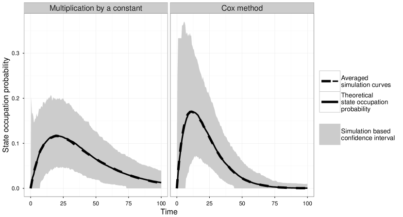
Figure 1: Results of the simulation study for the scenario “multiplication by a constant” in the left panel and the “Cox method” on the right. The solid black line represents the true state occupation probability, the dashed line the averaged probabilities obtained from the simulated studies. The grey area is the simulation based 95% confidence interval.

As can be seen, the curves can almost not be distinguished. Therefore, we can conclude that within these simulation designs the Aalen-Johansen estimator for the state occupation probability still performs well under random left-truncation.

3.2 The wild bootstrap resampling technique

Before we investigate more closely the performance of the landmark Aalen-Johansen estimator in the next section, we consider in this section the wild bootstrap resampling technique in non-Markov models and compare it with the standard Efron’s bootstrap. Moreover, to get a more complete picture of the performance of the wild bootstrap, we extend our evaluation to Markov models subject to type II censoring.
The key result, that allows us to apply the wild bootstrap in non-Markov models, is the consistent estimation of the cumulative transition hazard by the Nelson-Aalen estimator as shown in Theorem 2.1. Therefore, we focus in this section on the Nelson-Aalen estimator of the cumulative hazard of the 1 $\rightarrow$ 2 transition. Detailed information to the wild bootstrapping of the multivariate Nelson-Aalen estimator including the transformation onto the Aalen-Johansen estimator can be found in Bluhmki et al. (2018).
As a first step, we simulated data from an illness-death model without recovery as in the previous section. We introduce dependence between the waiting time in the initial state and the waiting time in the illness state by multiplying constant transition hazards by a common gamma frailty Z. Here, Z is a gamma-distributed random variable with mean and variance equal to 2. Moreover, we added exponentially distributed random right-censoring times. We use the following constant transition hazards: $\alpha_{01}=0.12$, $\alpha_{12}=0.1$, $\alpha_{02}=0.03$. We considered different sample sizes — 30, 50 and 100 individuals per study — and simulated 100 studies for each scenario. For the construction of point-wise 95% confidence intervals, we used two different resampling techniques — Efron’s bootstrap and the wild bootstrap technique. Both resampling methods are used to determine the $(1-\alpha/2)$ - quantiles of the standardized Nelson-Aalen estimator which were plugged-in in the standard asymptotic formula instead of using the quantiles of the standard normal distribution. We use the empirical variance of the bootstrapped Nelson-Aalen estimators as variance estimator. Table 1 compares the coverage probabilities of the 95% point-wise confidence intervals obtained from those two resampling methods for different sample sizes and at different time-points. Both methods provide coverage probabilities close to the nominal level of 95%. However, for the scenarios with a sample size of 30 individuals, the wild bootstrap approach still leads to coverage probabilities close to the nominal level, whereas the confidence intervals obtained by Efron’s bootstrap are quite liberal. In summary, under an i.i.d. data structure both resampling approaches provide reliable results in situations where the Markov property is in doubt. Our simulations indicate that for small sample sizes the wild bootstrap approach performs better compared to Efron’s bootstrap.
One big advantage of the wild bootstrap technique is, that it is, in contrast to Efron’s bootstrap, not limited to the strict situation with i.i.d. data structure. Thus, the wild bootstrap does not require random censoring. As the i.i.d. data structure is a requirement for the consistency of the Nelson-Aalen estimator in non-Markov models, we consider a Markov model subject to event-driven censoring, so-called type II censoring, to investigate the impact of the violation of the i.i.d. data assumption. In other words, the aim of the following simulation is to investigate possible advantages of wild bootstrapping when random censoring, but not the Markov property is in doubt. Type II censoring implies that all individuals will be censored at the time when a specified number of occurrences of the event of interest has been taken place. Thus, type II censoring is no random censoring but it fulfills the independent censoring assumption of Andersen et al. (1993) and Aalen et al. (2008), in that retains the form of the intensities of the counting processes as in (6).

In our simulation studies, we censored all individuals at the time when half of the individuals had an observed death event. We used constant hazard rates ($\alpha_{01}=0.01$, $\alpha_{12}=0.1$, $\alpha_{02}=0.03$) and no staggered study entry. That means all individuals enter the study at time 0. Table 2 shows the coverage probabilities of the 95 % confidence intervals constructed using the two different resampling methods at different time points and for different sample sizes. It can be seen that the wild bootstrap technique provides coverage probabilities closer to the nominal level compared to Efron’s bootstrap for all considered scenarios.

Table 1: Comparison of empirical coverage probabilities of the 95% point-wise confidence intervals constructed using Efron’s bootstrap and the wild bootstrap at different time-points in non-Markov illness death model

	Coverage (%)
	Efron			Wild Bootstrap
n	T15	T20	T25	T15	T20	T25
n=30	88	87	81	96	97	97
n=50	94	93	91	97	96	95
n=100	98	98	97	95	97	98

Table 2: Comparison of empirical coverage probabilities of the 95% point-wise confidence intervals constructed using Efron’s bootstrap and wild bootstrap at different time-points in Markov models subject to type II censoring with censoring after $m$ events have been observed.

		Coverage (%)
		Efron			Wild Bootstrap
n	m	T8	T12	T16	T8	T12	T16
n=80	m=40	71	83	87	88	98	97
n=100	m=50	81	87	87	94	97	97
n=200	m=100	88	91	93	93	92	95

3.3 The landmark Aalen-Johansen estimator

We now extend the simulation setting of Titman (2015) and Putter and Spitoni (2016). The data are simulated from an illness-death model without recovery. As in Titman, we consider two processes, termed ‘Frailty’ and ‘non-Markov’. The baseline transition hazards are constant, with $\alpha_{01}=0.12$, $\alpha_{02}=0.03$ and $\alpha_{12}=0.1$. For the ’Frailty’ model, all hazards are multiplied by a common gamma frailty $Z$ with mean and variance equal to 2. The frailty term introduces dependence between the waiting time until leaving the initial state of the illness-death model and the waiting time until absorption and, hence, a violation of the Markov assumption. In the ’non-Markov’ scenario, $\alpha_{12}(t)$ is dependent on the state occupied at time 4, i.e.,

$$\alpha_{12}(t)=\begin{cases}0.05,&\text{if }X(4)=0,\\ 0.1,&\text{otherwise}.\end{cases}$$

Transition times were simulated as in Section 3.1. We considered sample sizes $m=200$ and $m=500$. Then random left-truncation times following a Uniform distribution (Unif) with parameters $(-5,28)$ and $(-1,13)$ for the ‘Frailty’ and ‘non-Markov’ scenario, respectively. We consider also exponentially distributed left-truncation times with parameter $0.13$. Here, nobody is starting in the study at time 0. Table 3 reports number of individuals simulated ($m$), average number of individuals in the study ($\bar{n}$, $\bar{n}<m$ because of left-truncation), bias, root mean squared error (RMSE), and the empirical coverage probability of the 95% bootstrap quantile confidence interval (15) (Cov), for the Aalen-Johansen and landmark Aalen-Johansen estimates of $P_{01}(\tau_{0.15},\tau_{0.45})$, where $\tau_{0.15}$ and $\tau_{0.45}$ correspond to the 15th and 45th percentiles of the time-to-absorption distribution whose values are taken from the supplementary material of Titman (2015).

Table 3: Average number of individuals under study ($\bar{n}$), bias, root mean square error (RMSE), and coverage

			AJ			LMAJ
Trunc	$m$	$\bar{n}$	Bias	RMSE	Cov (%)	Bias	RMSE	Cov (%)
Simulation model ‘Frailty’
Unif	200	141	-0.0038	0.047	97	0.0001	0.069	92
	500	353	0.0003	0.028	97	0.0056	0.038	99
Exp	200	157	-0.0053	0.040	91	0.0015	0.051	96
	500	391	-0.0016	0.023	95	0.0008	0.032	97
Simulation model ‘non-Markov’
Unif	200	152	-0.0250	0.060	93	0.0087	0.083	97
	500	382	-0.0285	0.041	85	-0.0010	0.046	98
Exp	200	146	-0.0266	0.057	88	-0.0008	0.081	92
	500	362	-0.0280	0.043	89	-0.0040	0.048	93

As in Putter and Spitoni (2016), the landmark Aalen-Johansen performs well. The Aalen-Johansen estimator is slightly more biased but displays the smallest RMSE for most scenarios. Efron’s bootstrap provides confidence intervals with coverage probabilities close to the nominal level for the Aalen-Johansen estimator in the ‘Frailty’ model, whereas in the ‘non-Markov’ model the coverages of that estimator are more liberal. With regard to the landmark Aalen-Johansen estimator, the coverages are similar in both models.

An alternative to Efron’s bootstrap is the wild bootstrap resampling technique. As pointed out in Section 3.2, this approach is valid in non-Markov models and can be used to construct confidence intervals for the Nelson-Aalen estimator. Following the proceeding of Bluhmki et al. (2018), we assume that the wild bootstrap can be also applied for construction of confidence intervals for the landmark Aalen-Johansen estimator, but this is subject to further research.

3.4 Real data example: nosocomial infection and stay in hospital

We consider data on patients colonised by Methicillin-resistant staphylococcus aureus (MRSA) from a prospective cohort study in 12 surgical units at the University of Geneva Hospitals, Switzerland, between July 2004 and May 2006 (De Angelis et al., 2011). MRSA carriage is not necessarily detected upon hospital admission, because a positive MRSA screening result may come in ‘delayed’ in the sense that the positive laboratory result becomes available or known only after admission. Hence, our population of interest are patients colonised by MRSA, the time scale of interest is time since hospital admission and the left-truncation time is the time of detecting MRSA in the screening process. Colonised patients who are discharged or die before a positive screening result becomes available are not included in the study.

MRSA colonization may lead to MRSA infection in hospital, and the more severe or potentially life-threatening MRSA infections are observed most frequently in healthcare settings. In this context and in the presence of limited financial resources, possible measures of infection control are weighed against the costs associated with hospital-acquired infection (Muto et al., 2003). To this end, excess length of stay following the infection is typically considered to be the main cost driver (Graves et al., 2010).

However, quantifying excess length of stay is complicated by the fact that hospital-acquired MRSA infection is a time-dependent exposure and a simple retrospective comparison of the distribution of length of stay of the infected with that of the only colonised must overestimate the prolonging effect of the infection as a consequence of ‘immortal time bias’ (Beyersmann et al., 2008; Suissa, 2008). We address this difficulty as follows: Firstly, we model occurrence of hospital-acquired MRSA infection as an intermediate state in an illness-death multi-state model, in which the initial state represents colonization, intermediate state 1 infection and absorbing state 2 discharge from the hospital. Secondly, we use landmarking to compare the residual length of stay (in terms of the transition probabilities) of those in in the infectious state at the landmark with those still in the initial state of colonization.

Two remarks are in place: Firstly, an alternative modelling approach would be a cure model, where a ‘cure proportion’ of colonised patients ‘immune’ to infection accounts for the fact that only a fraction of the colonised patients are diagnosed with MRSA infection in hospital. This is in contrast to the multi-state approach where the interplay of the intensities out of the initial colonization state, one for infection, one for direct discharge, regulates the proportion of infected patients. One reason to choose a multi-state modelling approach was that not becoming infected may be a consequence of actions taken after a positive screening result such as decolonization (De Angelis et al., 2011). Secondly, landmarking has been introduced in medical research to deal with the difficulties of comparing groups defined by time-dependent exposures (Anderson et al., 1983, 2008), while the landmark Aalen-Johansen estimator of Putter and Spitoni (2016) and of our Section 3.3 has used landmarking for estimating transition probabilities rather than just state occupation probabilities. This further highlights the close connection between time-dependent exposures and multi-state modelling.

We begin our analysis by checking the Markov assumption using a Cox model, estimate the proportion of currently infected and hospitalized patients using the Aalen-Johansen estimator of state occupation probabilities and finally compare the residual length-of-stay distributions between infected and only colonised for different landmarks using the landmark Aalen-Johansen estimator of transition probabilities. Recall that all analyses must account for the data being subject to left-truncation.

In order to check the Markov assumption we include the time of infection in a Cox proportional hazards model for the hazard of end-of-stay (Keiding and Gill, 1990). The HR is found to be significantly smaller than 1 (HR: 0.98, 95%-CI [0.97, 0.99]). Thus the later one becomes infected the lower the hazard of being discharged.

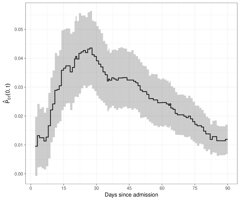
Figure 2: Estimated state occupation probability $P_{01}(0,t)$ for the MRSA data along with 95% point-wise confidence interval based on 1000 bootstrap samples.

Figure 2 displays the estimated probability to be in the infectious state, i.e., the state occupation probabilitybased on 1000 bootstrap samples. We note that this probability is low.

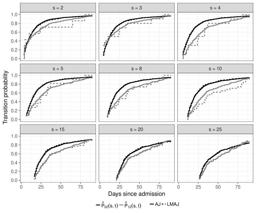
Figure 3: Landmark analysis of the MRSA data. Each panel displays $P_{02}(s,t)$ (black) and $P_{12}(s,t)$ (grey) for $s\in\{2,3,4,5,8,10,15,20,25\}$ estimated by the Aalen-Johansen estimator (solid lines) and the landmark Aalen-Johansen estimator (dashed lines).

Finally, Figure 3 provides a landmark analysis, displaying both landmark Aalen-Johansen estimates and the original Aalen-Johansen estimates of $P_{02}(s,t)$ and $P_{12}(s,t)$ for a selected range of landmark times
$s=\in\{2,3,4,5,8,10,15,20,25\},\,s<t$. The prolonging effect of MRSA is illustrated by the fact that $\hat{P}_{02}(s,t)$ runs above $\hat{P}_{12}(s,t)$ for all $s$, though this effect is much more pronounced for s between 8 and 15 days. We also see that for these data, the Aalen-Johansen and landmark Aalen-Johansen estimators are close to each other in spite of the data being possibly non-Markov.

4 Discussion

Multi-state modelling is useful for investigating complex courses of a disease in a variety of medical disciplines, but usually comes with a time-inhomogeneous Markov assumption to facilitate the technical developments. In particular, estimating transition probabilities when the Markov assumption is in doubt has been an active field of research in recent years. To the best of our knowledge, one of the first proposals is due to Meira-Machado et al. (2006) who used Kaplan-Meier integrals for a randomly right-censored illness-death model. Their approach was simplified by Allignol et al. (2014b) using competing risks techniques. Allignol et al. also used semi-parametric efficiency arguments to arrive at landmark transition probability estimators, also allowing for delayed study entry, see also Gerds et al. (2017). Their approach was then recently extended to arbitrary multi-state models by Titman (2015), see also de Uña-Álvarez and Meira-Machado (2015) for related work. Arguably the most natural approach is due to Putter and Spitoni (2016) using a landmark Aalen-Johansen estimator and consistency of the Aalen-Johansen estimator for state occupation probabilities of non-Markov multi-state models subject to random right-censoring. Our paper complements the work by Putter and Spitoni, establishing the consistency needed and extending results to delayed study entry which is a common phenomenon in observational studies. Our proof also motivates use of the wild bootstrap resampling method and shows its validity in non-Markov models using simulation studies. In contrast to Efron’s bootstrap the wild bootstrap is not limited to situations with i.i.d. data structure and, hence, could also be applied to censoring scenarios that are more complex than random censoring (Bluhmki et al., 2018), then, however, relying on the time-inhomogeneous Markov framework.

Acknowledgement

Jan Beyersmann was partially supported by Grant BE 4500/1-2 of the German Research Foundation (DFG).

Appendix A Proofs

• of Theorem 2.1

  To begin, note that we do not sample from $P$ but from the conditional probability measure given study entry $Q(\cdot)=P(\cdot\,|\,Z)$. Dropping indices $l$ as in $Y_{i;l}$ and $lm$ as in $N_{lm}$ denoting the transition type for ease of notation, we have that

  $$\hat{A}(t) = \int_{0}^{t}\frac{J(u)}{Y(u)}{\rm\;d}N(u)$$

  $$= \underbrace{\int_{0}^{t}\frac{J(u)}{Y(u)}{\rm\;d}M(u)}_{=M^{\star}(t)}+\underbrace{\int_{0}^{t}\frac{J(u)}{Y(u)}\sum_{i=1}^{n}Y_{i}(u)\cdot\alpha_{i}(u|\mathcal{G}(u-)){\rm\;d}u}_{=A^{\star}(t)}.$$

  $M^{\star}(t)$ is a mean zero martingale with predictable variation process

  $$V(t)=\int_{0}^{t}\frac{J(u)}{Y(u)^{2}}\sum_{i=1}^{n}Y_{i}(t)\cdot\alpha_{i}(u|\mathcal{G}(u-)){\rm\;d}u.$$

  Because of Lenglart’s inequality, we have that for any $\delta,\eta>0$

  $$Q\left(\sup_{[0,t]}|\hat{A}-A^{\star}|>\eta\right)\leq\frac{\delta}{\eta^{2}}+Q(V(t)>\delta).$$

  Assumption (8) implies

  $$V(t)\leq\int_{0}^{t}\frac{J(u)}{Y(u)}k(u){\rm\;d}u$$

  and it follows from (9) that

  $$\sup_{[0,t]}|\hat{A}-A^{\star}|\stackrel{{\scriptstyle Q}}{{\to}}0.$$

  To complete the proof, we still need to show

  $$\sup_{[0,t]}\left|\int_{0}^{t}\left\{\frac{J(u)}{Y(u)}\sum_{i=1}^{n}Y_{i}(u)\cdot\alpha_{i}(u|\mathcal{G}(u-))\right\}-\alpha(u){\rm\;d}u\right|\stackrel{{\scriptstyle Q}}{{\to}}0.$$ (16)

  Under assumption (8) and using Gill’s dominated convergence theorem (Andersen et al., 1993, Proposition II.5.3), it suffices to show point-wise convergence in probability of the integrand. We have

  $$\frac{Y(u)}{n}\stackrel{{\scriptstyle Q}}{{\to}}Q(Y_{1}(u)=1)=Q(Y_{i}(u)=1)\mbox{\ for all\ }i=1,\ldots,n.$$

  Next, note that the dependence of $\alpha_{i}(u|\mathcal{G}(u-))$ on the past of the observed data only constitutes dependence on $i$th observed past but not on that of other individuals $j$, $j\neq i$, because of independence across individuals. Using that left-truncation and right-censoring are random, we get that

  $$Y_{i}(u)\cdot\alpha_{i}(u|\mathcal{G}(u-)),i=1,\ldots,n,$$

  are i.i.d. random variables, and their average approaches the mean given by the following calculation

  $${\rm E}(Y_{i}(u)\cdot\alpha_{i}(u|\mathcal{G}(u-)){\rm\;d}u) = {\rm E}\big{(}{\rm E}\{Y_{i}(u)\cdot\alpha_{i}(u|\mathcal{G}(u-)){\rm\;d}u\}\,|\,\mathcal{G}(u-)\big{)}$$

  $$= {\rm E}\big{(}Q({\rm d}N_{i}(u)=1\,|\,\mathcal{G}(u-))\big{)}$$

  $$= Q({\rm d}N_{i}(u)=1)$$

  $$= Q(Y_{i}(u)=1)\cdot Q({\rm d}N_{i}(u)=1\,|\,Y_{i}(u)=1)$$

  and, recalling that we consider transitions $l\to m$,

  $$Q({\rm d}N_{i}(u)=1\,|\,Y_{i}(u)=1)$$

  $$= P(X_{i}(u+{\rm d}u)=m,u+{\rm d}u\leq C\,|\,X_{i}(u-)=l,L_{i}<u\leq C_{i})$$

  $$= P(X_{i}(u+{\rm d}u)=m\,|\,X_{i}(u-)=l)=\alpha(u){\rm\;d}u.$$

  In the previous display, the first equality holds, because $X_{i}(u-)=l,L_{i}<u$ implies study entry for a transient state $l$. Point-wise convergence of the integrand in (16) follows, which completes the proof.

• of Theorem 2.2

  The proof relies on the observation by Andersen et al. (Andersen et al., 1993, Section IV.4.1.4) for complete data that the entries of $\hat{p}(t)$ are the usual multinomial estimates, i.e., the number of trajectories observed in a specific state divided by $n$, if we chose $\hat{p}(0)$ as remarked after Theorem 2.2. In other words, Theorem 2.2 holds in the absence of both left-truncation and right-censoring.

  Now, because product integration is a continuous functional (or operator) (Gill and Johansen, 1990), the assertion will follow as a consequence of the continuous mapping theorem, if the Nelson-Aalen estimator consistently estimates the same limit in the presence of random left-truncation and right-censoring as it does in the complete data case. This is precisely what Theorem 1 states, which completes the proof. Here, we view the multivariate Nelson-Aalen estimator as a random element of $D[0,t]^{K^{2}+K}$, $t\leq\tau$, equipped with the max-supremum norm.

References

- Aalen et al. (2008) Aalen, O., Borgan, O., and Gjessing, H. (2008) Survival and event history analysis: a process point of view, Springer Science & Business Media.