Hermite spectral method for Fokker-Planck-Landau equation modeling collisional plasma

Abstract

We propose an Hermite spectral method for the Fokker-Planck-Landau (FPL) equation. Both the distribution functions and the collision terms are approximated by series expansions of the Hermite functions. To handle the complexity of the quadratic FPL collision operator, a reduced collision model is built by adopting the quadratic collision operator for the lower-order terms and the diffusive Fokker-Planck operator for the higher-order terms in the Hermite expansion of the reduced collision operator. The numerical scheme is split into three steps according to the Strang splitting, where different expansion centers are employed for different numerical steps to take advantage of the Hermite functions. The standard normalized Hermite basis [36] is adopted during the convection and collision steps to utilize the precalculated coefficients of the quadratic collision terms, while the one constituted by the local macroscopic velocity and temperature is utilized for the acceleration step, by which the effect of the external force can be simplified to an ODE. Projections between different expansion centers are achieved by an algorithm proposed in [29]. Several numerical examples are studied to test and validate our new method.

keyword: quadratic collision operator, Hermite spectral method, Strang splitting

1 Introduction

The Fokker-Planck-Landau (FPL) equation is used to describe the evolution of collisional plasma systems at the kinetic level [25, 15]. It is a six-dimensional integro-differential equation, which models binary collisions between charged particles with long-range Coulomb interactions. The FPL equation is the limit of the Boltzmann equation when all binary collisions are grazing [14]. It was originally derived by Landau [32] and was later derived independently in the Fokker-Planck form [41]. The high-dimensionality of the FPL equation is a bottleneck for its numerical simulations. Although several simplified models of the original FPL equation has been developed, it is still a challenge to solve it both fast and accurately.

One of the major difficulties in solving FPL equation numerically is the complexity of the Fokker-Planck collision operator, which is an integro-differential nonlinear operator in the microscopic velocity space. Most of the statistical methods, such as the DSMC method [2], are limited for the FPL equation [37] since the FPL collision operator models the infinite-range potential interactions within the plasma. Several deterministic methods are used to solve the FPL equation or its simplifications. The entropic scheme, which guarantees a nondecreasing entropy, is well studied in [34, 5, 1, 15]. To handle the stiffness of the collision operator, an asymptotic-preserving (AP) strategy is studied in [18], while a conservative spectral method is adopted in [53]. A positivity-preserving scheme for the linearized FPL equation is proposed in [9], after which it was modified to preserve energy [31] and then extended to the two-dimensional FPL equation with cylindrical geometry [50]. Several other numerical methods, such as the multipole expansions [33] and multigrid techniques [6], have also been proposed. In [45], a fully implicit method is proposed for the multidimensional Rosenbluth-Fokker-Planck equation. The finite element methods in [52, 51] and the semi-Lagrangian schemes in [13, 44, 40, 49] are also used to solve the Vlasov equations. Moreover, the FPL equation with stochasticity is studied in [19].

The spectral method has been widely used in numerical methods to solve the Vlasov equation [23, 27]. In [38, 20], a spectral method based on the Fourier expansion is implemented for the nonhomogeneous FPL equation. Moreover, the Hermite spectral method is utilized in [4, 39, 24] to discretize the microscopic velocity space and is utilized to solve the FPL and Boltzmann equation [29]. One advantage of the Hermite spectral method is that its first few moments have explicit physical meanings. For example, the density, the macroscopic velocity and the temperature can be easily derived using the first three expansion coefficients [38], which indicates that they may be captured more precisely by ingeniously designing the numerical algorithm. However, the high-dimensionality and complexity of the quadratic FPL collision model still impose great challenges for adopting the Hermite spectral method to numerically simulate the FPL equation.

In this paper, a numerical method based on the Hermite spectral method is proposed for the nonhomogeneous FPL equation. The distribution functions in the FPL equation are approximated by a series of basis functions derived from Hermite polynomials. Strang splitting method is then adopted for the FPL equation, which is split into collision, convection and acceleration steps. Unlike the general Hermite spectral method [38], we choose different expansion centers in the Hermite expansion for different numerical steps. For the collision step, the standard expansion center [36] is chosen to utilize the precalculated expansion coefficients of the quadratic collisional term. To further reduce the computational cost of the quadratic FPL collision operator, a reduced collision model is constructed by combining the quadratic collision operator and the diffusive FP operator, which is proved effective by the numerical examples afterwards. For the acceleration step, the expansion center is chosen as the local macroscopic velocity and temperature, under which the effect of the external force field can be reduced to an ODE of the macroscopic velocity. A projection algorithm introduced in [29] is utilized to handle the projections between distribution functions with different expansion centers. In the numerical simulation, the convection, collision and acceleration steps are solved successively. Both the linear and nonlinear Landau damping problems are tested, with the decay rate of the electrostatic energy and the effect of the collisional frequency studied. Moreover, the two-stream instability and the bump-on-tail instability are also simulated to validate this new method.

The rest of this paper is organized as follows: Section 2 introduces the FPL equation, the FPL collision operator and several related properties. The detailed spectral method used to approximate the distribution function is introduced in Section 3. The series expansion for the FPL collision operator and the reduced collision model are explained in Section 4. The numerical algorithm is proposed in Section 5. Several numerical examples are exhibited in Section 6. The conclusions and future work are stated in Section 7 with some supplementary statements given in the Appendix 8.

2 Preliminaries

In this section, we give a brief introduction to the Fokker-Planck-Landau equation, the Fokker-Planck collision operator and some related properties.

2.1 Fokker-Planck-Landau equation

As in many other kinetic theories in physics, the distribution function of a specific species $\alpha$ is described by the distribution function $f_{\alpha}(t,\bm{x},\bm{v})$, a seven-dimensional function of time $t$, the space position $\bm{x}\in\Omega\subset\mathbb{R}^{3}$ and the microscopic velocity $\bm{v}\in\mathbb{R}^{3}$. The distribution function $f_{\alpha}$ relates the density $\rho_{\alpha}$, the macroscopic velocity $\bm{u}_{\alpha}$ and the temperature $T_{\alpha}$ of species $\alpha$ through

$$\rho_{\alpha} =\int_{\mathbb{R}^{3}}f_{\alpha}(t,\bm{x},\bm{v})\,\mathrm{d}\bm{v},\quad\rho_{\alpha}\bm{u}_{\alpha} =\int_{\mathbb{R}^{3}}\bm{v}f_{\alpha}(t,\bm{x},\bm{v})\,\mathrm{d}\bm{v},\quad\frac{3}{2}\rho_{\alpha}T_{\alpha} =\frac{1}{2}\int_{\mathbb{R}^{3}}|\bm{v}-\bm{u}_{\alpha}|^{2}f_{\alpha}(t,\bm{x},\bm{v})\,\mathrm{d}\bm{v}.$$ (2.1)

The Fokker-Planck-Landau (FPL) equation describes the time evolution of the distribution functions for charged particles in a nonequilibrium plasma. The FPL equation with respect to the species $\alpha$ has the form

$$\dfrac{\partial{f_{\alpha}}}{\partial{t}}+\bm{v}\cdot\nabla_{\bm{x}}f_{\alpha}+\bm{F}\cdot\nabla_{\bm{v}}f_{\alpha}=\mathcal{Q}[f_{\alpha}],$$ (2.2)

where the force field $\bm{F}=\bm{F}(t,\bm{x})$ is produced either externally or self-consistently. Here, we consider only the case where $\bm{F}$ is generated by the self-consistent electric field $\bm{E}(t,\bm{x})$, which is coupled to the distribution function through the Poisson equation [22]:

$$\bm{E}(t,\bm{x})=-\nabla_{\bm{x}}\psi(t,\bm{x}),\qquad-\Delta_{\bm{x}}\psi=\sum_{\eta}q_{\eta}\int_{\mathbb{R}^{3}}f_{\eta}(\bm{v})\,\mathrm{d}\bm{v},$$ (2.3)

where $q_{\eta}$ is the electric charge of the particle $\eta$. The collision terms

$$\mathcal{Q}[f_{\alpha}]=\sum_{\eta}\nu_{\eta}\mathcal{Q}_{\eta}[f_{\alpha},f_{\eta}]$$ (2.4)

describe the collisions between particles of species $\alpha$ and $\eta$, which are discussed in detail in the next section. The non-negative parameter $\nu_{\eta}$ is the collision frequency. For simplicity, we restrict the study to a plasma consisting only of electrons and ions, which are referred to as the species $\alpha$ and $\beta$ respectively, in the following.

2.2 Collision operator

The collision operator $\mathcal{Q}_{\eta}$, $\eta=\alpha,\beta$ in (2.4) is called the Fokker-Planck-Landau (FPL) collision operator, which is obtained by setting the Boltzmann collision operator concentrating on grazing collisions [16]. It has the following form:

$$\mathcal{Q}_{\eta}[f_{\alpha},f_{\eta}]=\nabla_{\bm{v}}\cdot\left[\int_{\mathbb{R}^{3}}{\bf A}(\bm{v}-\bm{v}^{\prime})\Big{(}\nabla_{\bm{v}}f_{\alpha}(\bm{v})f_{\eta}(\bm{v}^{\prime})-\nabla_{\bm{v}^{\prime}}f_{\eta}(\bm{v}^{\prime})f_{\alpha}(\bm{v})\Big{)}\,\mathrm{d}\bm{v}^{\prime}\right],\qquad\eta=\alpha,\beta,$$ (2.5)

where the collision kernel $\bf A(\cdot)$, in the form of a $3\times 3$ negative and symmetric matrix

$${\bf A}(\bm{v})=\Psi(|\bm{v}|)\Pi(\bm{v}),$$ (2.6)

reflects the interaction between particles. Here $\Pi(\bm{v})$ is the projection onto the space orthogonal to $\bm{v}$, as $\Pi_{ij}(\bm{v})=\delta_{ij}-\frac{v_{i}v_{j}}{|\bm{v}|^{2}}$. For the inverse-power-law (IPL) model, $\Psi(|\bm{v}|)$ is a non-negative radial function, i.e.

$$\Psi(\bm{v})=\Lambda|\bm{v}|^{\gamma+2},$$ (2.7)

where $\Lambda$ is a positive constant and $\gamma$ is the index of the power of the distance. Similar to the Boltzmann equation, we obtain the hard potential model when $\gamma>0$ and the soft potential model when $\gamma<0$. There are two special cases, the first of which is the model of Maxwell molecules when $\gamma=0$ and the other is the model with Coulomb interactions when $\gamma=-3$ [20].

For the different species of electrons and ions, the collision operator (2.5) may be reduced to different forms. These two collision operators are discussed in detail below.

2.2.1 Electron-electron collision

The quadratic operator $\mathcal{Q}_{\alpha}[f_{\alpha},f_{\alpha}]$ describes the electron-electron collisions, the form of which can be obtained by taking $\eta$ as $\alpha$ in the FPL collision operator (2.5). With a slight abuse of notation, the subscript $\alpha$ referring electrons is omitted from now on. Thus, the distribution function $f_{\alpha}$ is shorten to $f$ and the collision operator $\mathcal{Q}_{\alpha}[f_{\alpha},f_{\alpha}]$ is shorten to $\mathcal{Q}[f,f]$ as

$$\mathcal{Q}[f,f]=\nabla_{\bm{v}}\cdot\left[\int_{\mathbb{R}^{3}}{\bf A}(\bm{v}-\bm{v}^{\prime})\Big{(}\nabla_{\bm{v}}f(\bm{v})f(\bm{v}^{\prime})-\nabla_{\bm{v}^{\prime}}f(\bm{v}^{\prime})f(\bm{v})\Big{)}\,\mathrm{d}\bm{v}^{\prime}\right],$$ (2.8)

with the collision kernel ${\bf A}(\cdot)$ defined in (2.6). For the steady solution of the FPL equation, we obtain the equilibrium, which has the following Maxwellian form:

$$\mathcal{M}(\bm{v})=\frac{\rho}{(2\pi T)^{3/2}}\exp\left(-\frac{|\bm{v}-\bm{u}|^{2}}{2T}\right),$$ (2.9)

where $\rho$, $\bm{u}$ and $T$ are the density, macroscopic velocity and temperature of electrons respectively (2.1). Moreover, this operator maintains the conservation of mass, momentum and energy as

$$\int_{\mathbb{R}^{3}}\mathcal{Q}[f,f]\left(\begin{array}[]{c}1\\ \bm{v}\\ |\bm{v}|^{2}\end{array}\right)\,\mathrm{d}\bm{v}=0.$$ (2.10)

Due to the complicated form of the FPL collision operator, several simplified operators are introduced to approximate the original quadratic operator $\mathcal{Q}[f,f]$, for example the linearized collision operator

$$\mathcal{L}[f]=\mathcal{Q}[f,\mathcal{M}]+\mathcal{Q}[\mathcal{M},f],$$ (2.11)

and the diffusive Fokker-Planck (FP) operator [30]

$$\mathcal{P}_{\rm FP}[f]=\nabla_{\bm{v}}\cdot\left[\mathcal{M}\nabla_{\bm{v}}\left(\frac{f}{\mathcal{M}}\right)\right].$$ (2.12)

2.2.2 Electron-ion collision

The collisions between electrons and ions are described by the operator $\mathcal{Q}_{\beta}[f,f_{\beta}]$, which can be obtained by taking $\eta$ as $\beta$ in (2.5). Since the electrons have a minute mass and high velocity compared to the ions, the ions may be collectively treated as a stationary positively-charged background. Furthermore, the temperature of ions $T_{\beta}$ is negligible compared to that of electrons $T$. Thus, the distribution function of ions can be given simply by a Dirac measure in the velocity space [53] as

$$f_{\beta}(t,\bm{x},\bm{v})=\rho_{\beta}(t,\bm{x})\delta_{0}(\bm{v}-\bm{u}_{\beta}(t,\bm{x})),$$ (2.13)

where $\rho_{\beta}$ and $\bm{u}_{\beta}$ are the density and macroscopic velocity of ions. Consequently, the collision operator $\mathcal{Q}_{\beta}[f,f_{\beta}]$ can be reduced to

$$\mathcal{Q}_{\beta}[f]\triangleq\mathcal{Q}_{\beta}[f,f_{\beta}]=\rho_{\beta}\nabla_{\bm{v}}\cdot\left[{\bf A}(\bm{v}-\bm{u}_{\beta})\nabla_{\bm{v}}f\right].$$ (2.14)

One can also easily check that this reduced operator still preserves mass and energy as

$$\int_{\mathbb{R}^{3}}\mathcal{Q}_{\beta}[f]\,\mathrm{d}\bm{v}=0,\qquad\int_{\mathbb{R}^{3}}|\bm{v}-\bm{u}_{\beta}|^{2}\mathcal{Q}_{\beta}[f]\,\mathrm{d}\bm{v}=0.$$ (2.15)

Refer to [12, 18] for more details on this reduced collision operator.

3 Series expansion of the FPL equation

In this section, we introduce the series expansion to approximate the distribution function in detail, including the basis functions which are constructed by Hermite polynomials and several related properties. In the numerical scheme, different expansion centers are utilized in the Hermite expansion. A fast algorithm for the projections between distribution functions with different expansion centers is also stated in this section.

3.1 Distribution function

The Hermite expansion has been proved successful in the numerical method for the Boltzmann equation [29], and the exact expansion coefficients for the quadratic FPL collision have been computed in [36]. Thus, the Hermite expansion is also adopted in the approximation to the FPL equation here. To be precise, the distribution function $f$ is discretized as

$$f(t,\bm{x},\bm{v})=\sum_{\bm{i}\in\mathbb{N}^{3}}f_{\bm{i}}^{[\tilde{\bm{u}},\tilde{T}]}(t,\bm{x})\mathcal{H}_{\bm{i}}^{[\tilde{\bm{u}},\tilde{T}]}(\bm{v}),$$ (3.1)

where the basis functions $\mathcal{H}_{\bm{i}}^{[\tilde{\bm{u}},\tilde{T}]}(\bm{v})$ are defined as

$$\mathcal{H}_{\bm{i}}^{[\tilde{\bm{u}},\tilde{T}]}(\bm{v})=\tilde{T}^{-\frac{|\bm{i}|}{2}}H_{\bm{i}}\left(\frac{\bm{v}-\tilde{\bm{u}}}{\sqrt{\tilde{T}}}\right)\frac{1}{(2\pi\tilde{T})^{3/2}}\exp\left(-\frac{|\bm{v}-\tilde{\bm{u}}|^{2}}{2\tilde{T}}\right)$$ (3.2)

and $\bm{i}$ refers to the multi-index $(i_{1},i_{2},i_{3})$. We also adopt the following notations for simplicity:

$$|\bm{i}|=i_{1}+i_{2}+i_{3},\qquad\bm{i}!=i_{1}!i_{2}!i_{3}!,\qquad\dfrac{\partial{{}^{\bm{i}}}}{\partial{\bm{v}^{\bm{i}}}}=\dfrac{\partial{{}^{i_{1}+i_{2}+i_{3}}}}{\partial{v_{1}^{i_{1}}v_{2}^{i_{2}}v_{3}^{i_{3}}}}.$$

In (3.2), $H_{\bm{i}}(\bm{v})$ represents the Hermite polynomial

$$H_{\bm{i}}(\bm{v})=(-1)^{|\bm{i}|}\exp\left(\frac{|\bm{v}|^{2}}{2}\right)\dfrac{\partial{{}^{\bm{i}}}}{\partial{\bm{v}^{\bm{i}}}}\left[\exp\left(-\frac{|\bm{v}|^{2}}{2}\right)\right],$$ (3.3)

where the two parameters $\tilde{\bm{u}}\in\mathbb{R}^{3}$ and $\tilde{T}\in\mathbb{R}_{+}$, namely the expansion center, are of the same dimension as $\bm{v}$ and $T$. The coefficients $f_{\bm{i}}^{[\tilde{\bm{u}},\tilde{T}]}$ can be explicitly expressed by

$$f_{\bm{i}}^{[\tilde{\bm{u}},\tilde{T}]}(t,\bm{x})=\dfrac{\tilde{T}^{\frac{|\bm{i}|}{2}}}{\bm{i}!}\int_{\mathbb{R}^{3}}f(t,\bm{x},\bm{v})H_{\bm{i}}\left(\dfrac{\bm{v}-\tilde{\bm{u}}}{\sqrt{\tilde{T}}}\right)\,\mathrm{d}\bm{v}$$ (3.4)

from the orthogonality of Hermite polynomials

$$\int_{\mathbb{R}^{3}}H_{\bm{i}}(\bm{v})H_{\bm{j}}(\bm{v})\exp\left(-\frac{|\bm{v}|^{2}}{2}\right)\,\mathrm{d}\bm{v}=\begin{cases}\bm{i}!,&\text{if }\bm{i}=\bm{j},\\ 0,&\text{otherwise.}\end{cases}$$ (3.5)

Several lower-order moments have close relations to macroscopic variables. For example, relations (2.1) with respect to density $\rho$, macroscopic velocity $\bm{u}$ and temperature $T$ of the electron can be rewritten by the expansion coefficients as

$$\begin{gathered}\rho=f_{\bm{0}}^{[\tilde{\bm{u}},\tilde{T}]},\qquad\rho\bm{u}=\rho\tilde{\bm{u}}+\left(f_{\bm{e}_{1}}^{[\tilde{\bm{u}},\tilde{T}]},f_{\bm{e}_{2}}^{[\tilde{\bm{u}},\tilde{T}]},f_{\bm{e}_{3}}^{[\tilde{\bm{u}},\tilde{T}]}\right)^{T},\\ \frac{1}{2}\rho|\bm{u}|^{2}+\frac{3}{2}\rho T=\rho\bm{u}\cdot\tilde{\bm{u}}-\frac{1}{2}\rho|\tilde{\bm{u}}|^{2}+\frac{3}{2}\rho\tilde{T}+\sum_{d=1}^{3}f_{2\bm{e}_{d}}^{[\tilde{\bm{u}}.\tilde{T}]}.\end{gathered}$$ (3.6)

Some other related macroscopic quantities such as the shear stress and the heat flux can also be expressed in terms of the expansion coefficients $f_{\bm{i}}^{[\tilde{\bm{u}},\tilde{T}]}$, and we refer [36] for further details. Moreover, it is worth mentioning that if the expansion parameters chosen are the local macroscopic velocity and temperature of the particles, i.e. $\tilde{\bm{u}}=\bm{u}$ and $\tilde{T}=T$, it holds that according to (3.6),

$$f_{\bm{e}_{d}}^{[\bm{u},T]}=0,\qquad\sum\limits_{d=1}^{3}f_{2\bm{e}_{d}}^{[\bm{u},T]}=0,\qquad d=1,2,3.$$ (3.7)

3.2 Projections between different expansion centers

One should be aware that different expansion centers may lead to different series expansions in (3.1) and can be selected to meet different needs. Based on a prior understanding of the problem, different expansion centers $\tilde{\bm{u}}$ and $\tilde{T}$ are chosen to accelerate the convergence of the series expansion (3.1).

The selection of expansion centers is discussed in many studies. The normalized Hermite basis, or the expansion center $\tilde{\bm{u}}=0$ and $\tilde{T}=1$, is adopted in [42, 39, 22], while the local macroscopic variables $\tilde{\bm{u}}=\bm{u}(t,\bm{x})$ and $\tilde{T}=T(t,\bm{x})$ defined in (2.1) are chosen as the expansion center in [8] and for some related problems [29]. Here, instead of fixing the expansion center throughout, we select an appropriate one for each numerical step. Here, instead of fixing the expansion center throughout, as we mainly focus on the reduction in the complexity of the series expansions and the feasibility of the numerical method, we select an appropriate one for each numerical step, which is further explained in Section 4 and 5.

To achieve efficient projections between distribution functions with different expansion centers, we adopt the algorithm proposed in [29], which is described by the following theorem:

Theorem 1.

Suppose a distribution function $f(\bm{v})$ in the velocity space satisfies

$$\int_{\mathbb{R}^{3}}(1+|\bm{v}|^{M})|f(\bm{v})|\,\mathrm{d}\bm{v}<\infty$$ (3.8)

for some $M\in\mathbb{Z}_{+}$.

Define the expansion coefficients of $f(\bm{v})$ as

$$f_{\bm{i}}^{[\tilde{\bm{u}}^{(1)},\tilde{T}^{(1)}]}=\frac{(\tilde{T}^{(1)})^{\frac{|\bm{i}|}{2}}}{\bm{i}!}\int_{\mathbb{R}^{3}}H_{\bm{i}}\left(\frac{\bm{v}-\tilde{\bm{u}}^{(1)}}{\sqrt{\tilde{T}^{(1)}}}\right)f(\bm{v})\,\mathrm{d}\bm{v},$$ (3.9)

$$f_{\bm{i}}^{[\tilde{\bm{u}}^{(2)},\tilde{T}^{(2)}]}=\frac{(\tilde{T}^{(2)})^{\frac{|\bm{i}|}{2}}}{\bm{i}!}\int_{\mathbb{R}^{3}}H_{\bm{i}}\left(\frac{\bm{v}-\tilde{\bm{u}}^{(2)}}{\sqrt{\tilde{T}^{(2)}}}\right)f(\bm{v})\,\mathrm{d}\bm{v}.$$

with $\tilde{\bm{u}}^{(s)}=\left(\tilde{u}^{(s)}_{1},\tilde{u}^{(s)}_{2},\tilde{u}^{(s)}_{3}\right),s=1,2\in\mathbb{R}^{3}$ and $\tilde{T}^{(1)},\tilde{T}^{(2)}>0$. Then, for any $\bm{i}\in\mathbb{N}^{3}$ satisfying $|\bm{i}|\leqslant M$, we have

$$f_{\bm{i}}^{[\tilde{\bm{u}}^{(2)},\tilde{T}^{(2)}]}=\sum_{l=0}^{|\bm{i}|}\phi_{\bm{i}}^{(l)}.$$ (3.10)

Here $\phi_{\bm{i}}^{(l)}$ is defined recursively by

$$\phi_{\bm{i}}^{(l)}=\begin{cases}f_{\bm{i}}^{[\tilde{\bm{u}}^{(1)},\tilde{T}^{(1)}]},&l=0,\\ \dfrac{1}{l}\sum\limits_{d=1}^{3}\left(\left(\tilde{u}^{(2)}_{d}-\tilde{u}^{(1)}_{d}\right)\phi_{\bm{i}-\bm{e}_{d}}^{(l-1)}+\frac{1}{2}(\tilde{T}^{(2)}-\tilde{T}^{(1)})\phi_{\bm{i}-2\bm{e}_{d}}^{(l-1)}\right),&1\leqslant l\leqslant|\bm{i}|,\end{cases}$$ (3.11)

where terms with negative indices are treated as zero.

We refer to Theorem 3.1 in [29] for the proof and more details of this projection algorithm.

4 Series expansion of the collision operators and the reduced collision model

For the moment, we have obtained the series approximation to the distribution function. In this section, the FPL collision operator (2.5) is expanded using the same basis functions. We derive the series expansions and provide algorithms to compute the expansion coefficients of the quadratic collision operator $\mathcal{Q}[f,f]$ (2.8) as well as its simplified approximation $\mathcal{P}_{\rm FP}$ and the collision operator between different species $\mathcal{Q}_{\beta}[f]$ (2.14) in this section.

Moreover, since the computational cost for the quadratic collision operator (2.5) is unaffordable, a reduced collision model is built based on the expansion coefficients to further reduce the computational cost.

4.1 Quadratic collision operator $\mathcal{Q}[f,f]$

As stated in Section 2.2, the major difficulty of handling the original FPL collision operator or even solving the FPL equation is the complexity of the quadratic collision operator $\mathcal{Q}[f,f]$. In our method, both precalculation and model reduction are employed to address this difficulty.

The quadratic collision operator $\mathcal{Q}[f,f]$ is to be expanded similarly to the series expansion of the distribution functions as

$$\mathcal{Q}[f,f](t,\bm{x},\bm{v})=\sum_{\bm{i}\in\mathbb{N}^{3}}Q_{\bm{i}}^{[\tilde{\bm{u}},\tilde{T}]}(t,\bm{x})\mathcal{H}_{\bm{i}}^{[\tilde{\bm{u}},\tilde{T}]}(\bm{v}).$$ (4.1)

By the orthogonality (3.5), the coefficients are calculated as

$$Q_{\bm{i}}^{[\tilde{\bm{u}},\tilde{T}]}(t,\bm{x})=\frac{\tilde{T}^{\frac{|\bm{i}|}{2}}}{\bm{i}!}\int_{\mathbb{R}^{3}}H_{\bm{i}}\left(\frac{\bm{v}-\tilde{\bm{u}}}{\sqrt{\tilde{T}}}\right)\mathcal{Q}[f,f](t,\bm{x},\bm{v})\,\mathrm{d}\bm{v}.$$ (4.2)

In our previous work [36], an algorithm was proposed to evaluate these coefficients in the standard case of $\rho=1,\tilde{\bm{u}}=\bm{0}$ and $\tilde{T}=1$, and the normalized Hermite basis was used to approximate the distribution function. To apply the results, the same expansion center is adopted here. Then, the approximation to the distribution function (3.1) and the collision operator (4.1) are reduced to

$$f(t,\bm{x},\bm{v}) =\sum_{\bm{i}\in\mathbb{N}^{3}}f_{\bm{i}}^{[\bm{0},1]}(t,\bm{x})\mathcal{H}_{\bm{i}}^{[\bm{0},1]}(\bm{v}),$$ (4.3)

$$\mathcal{Q}[f,f](t,\bm{x},\bm{v}) =\sum_{\bm{i}\in\mathbb{N}^{3}}Q_{\bm{i}}^{[\bm{0},1]}(t,\bm{x})\mathcal{H}_{\bm{i}}^{[\bm{0},1]}(\bm{v}).$$ (4.4)

The superscript $[\bm{0},1]$ is omitted afterwards if the expansion center $\tilde{\bm{u}}=\bm{0}$ and $\tilde{T}=1$ is used. Thus, in this case, the coefficients (4.2) are reduced to

$$Q_{\bm{i}}(t,\bm{x})=\frac{1}{\bm{i}!}\int_{\mathbb{R}^{3}}H_{\bm{i}}\left(\bm{v}\right)\mathcal{Q}[f,f](t,\bm{x},\bm{v})\,\mathrm{d}\bm{v}.$$ (4.5)

Substituting (4.3) into (4.5), we can derive that

$$Q_{\bm{i}}(t,\bm{x}) =\frac{1}{\bm{i}!}\int_{\mathbb{R}^{3}}H_{\bm{i}}\left(\bm{v}\right)\nabla_{\bm{v}}\cdot\left[\int_{\mathbb{R}^{3}}{\bf A}(\bm{v}-\bm{v}^{\prime})\big{(}f(\bm{v}^{\prime})\nabla_{\bm{v}}f(\bm{v})-f(\bm{v})\nabla_{\bm{v}^{\prime}}f(\bm{v}^{\prime})\big{)}\,\mathrm{d}\bm{v}^{\prime}\right]\,\mathrm{d}\bm{v}$$ (4.6)

$$=\sum_{\bm{j}\in\mathbb{N}^{3}}\sum_{\bm{k}\in\mathbb{N}^{3}}A_{\bm{i}}^{\bm{j},\bm{k}}f_{\bm{j}}f_{\bm{k}},$$

where the coefficients $A_{\bm{i}}^{\bm{j},\bm{k}}$ have the following expression [36, Eq.(3.4)]:

$$A_{\bm{i}}^{\bm{j},\bm{k}}=\dfrac{1}{\bm{i}!}\int_{\mathbb{R}^{3}}H_{\bm{i}}(\bm{v})\nabla_{\bm{v}}\cdot\left[\int_{\mathbb{R}^{3}}A(\bm{v}-\bm{v}^{\prime})(\mathcal{H}_{\bm{j}}(\bm{v}^{\prime})\nabla_{\bm{v}}(\mathcal{H}_{\bm{k}}(\bm{v}))-\mathcal{H}_{\bm{j}}(\bm{v})\nabla_{\bm{v}^{\prime}}(\mathcal{H}_{\bm{k}}(\bm{v}^{\prime}))\,\mathrm{d}\bm{v}^{\prime}\,\mathrm{d}\bm{v}\right].$$ (4.7)

Although the complicated form of the coefficients $A_{\bm{i}}^{\bm{j},\bm{k}}$ results in a formidably high computational cost, we find that these coefficients are intrinsic to the collision model and are constant when a specific collision model is chosen, which in our case means that the index $\gamma$ in the IPL model (2.7) is fixed. This indicates that we can always precalculate these coefficients completely offline once and then use them in all cases. In [36], an algorithm was proposed to calculate accurate values of the coefficients $A_{\bm{i}}^{\bm{j},\bm{k}}$ (or $A_{\alpha}^{\lambda,\kappa}$ correspondingly in [36, Eq.(3.4)]) by introducing Burnett polynomials for all $\gamma>-5$. Due to the lengthy expressions involved in the algorithm, we do not present the details here. Readers may refer to Theorem 1, Lemma 2, Proposition 3 and Theorem 4 in [36] for the details of this algorithm.

Moreover, utilizing the recurrence relations of the Hermite polynomial

$$\begin{gathered}\dfrac{\partial}{\partial v_{d}}H_{\bm{i}}(\bm{v})=i_{d}H_{\bm{i}-\bm{e}_{d}}(\bm{v}),\quad H_{\bm{i}+\bm{e}_{d}}(\bm{v})=v_{d}H_{\bm{i}}(\bm{v})-i_{d}H_{\bm{i}-\bm{e}_{d}}(\bm{v}),\\ \dfrac{\partial}{\partial v_{d}}\left[H_{\bm{i}}(\bm{v})\exp\left(-\frac{|\bm{v}|^{2}}{2}\right)\right]=-H_{\bm{i}+\bm{e}_{d}}(\bm{v})\exp\left(-\frac{|\bm{v}|^{2}}{2}\right),\qquad d=1,2,3,\end{gathered}$$ (4.8)

the diffusive FP operator $\mathcal{P}_{\rm FP}[f]$ (2.12), a simplified approximation to the quadratic collision operator $\mathcal{Q}[f,f]$, can also be expanded as

$$\mathcal{P}_{\rm FP}[f]=\sum_{\bm{i}\in\mathbb{N}^{3}}{\rm FP}_{\bm{i}}\mathcal{H}_{\bm{i}}(\bm{v}),\qquad{\rm FP}_{\bm{i}}=\sum_{d=1}^{3}\left[\left(1-\frac{1}{T}\right)f_{\bm{i}-2\bm{e}_{d}}+\frac{u_{d}}{T}f_{\bm{i}-\bm{e}_{d}}\right]-\frac{|\bm{i}|}{T}f_{\bm{i}},$$ (4.9)

where $\bm{u}=(u_{1},u_{2},u_{3})^{T}$ and $T$ are the macroscopic velocity and temperature of electrons (2.1), respectively.

4.2 Collision operator $\mathcal{Q}_{\beta}[f]$

The collision operator $\mathcal{Q}_{\beta}[f]$ (2.14) between different species can also be expanded with similar methods. Without loss of generality, we set $\rho_{\beta}=1$. Therefore, the collision operator $\mathcal{Q}_{\beta}[f]$ is expanded as

$$\mathcal{Q}_{\beta}[f](t,\bm{x},\bm{v})=\sum_{\bm{i}\in\mathbb{N}^{3}}\mathcal{Q}_{\beta,\bm{i}}^{[\tilde{\bm{u}},\tilde{T}]}(t,\bm{x})\mathcal{H}_{\bm{i}}^{[\tilde{\bm{u}},\tilde{T}]}(\bm{v}),$$ (4.10)

with the coefficients being

$$\mathcal{Q}_{\beta,\bm{i}}^{[\tilde{\bm{u}},\tilde{T}]}(t,\bm{x}) =\frac{1}{\bm{i}!}\int_{\mathbb{R}^{3}}\mathcal{Q}_{\beta}[f](t,\bm{x},\bm{v})H_{\bm{i}}\left(\frac{\bm{v}-\tilde{\bm{u}}}{\sqrt{\tilde{T}}}\right)\,\mathrm{d}\bm{v}$$ (4.11)

$$=\frac{1}{\bm{i}!}\int_{\mathbb{R}^{3}}\nabla_{\bm{v}}\cdot\left[{\bf A}(\bm{v}-\bm{u}_{\beta})\nabla_{\bm{v}}f\right]H_{\bm{i}}\left(\frac{\bm{v}-\tilde{\bm{u}}}{\sqrt{\tilde{T}}}\right)\,\mathrm{d}\bm{v}.$$

Noting that the macroscopic velocity $\bm{u}_{\beta}$ of ions appears in the expression of the collision operator $\mathcal{Q}_{\beta}[f]$, the expansion center here is chosen as $\tilde{\bm{u}}=\bm{u}_{\beta}$ and $\tilde{T}=1$ to simplify its series expansion. Thus, (4.10) and (4.11) are reduced to

$$\mathcal{Q}_{\beta}[f](t,\bm{x},\bm{v})=\sum_{\bm{i}\in\mathbb{N}^{3}}\mathcal{Q}_{\beta,\bm{i}}^{[\bm{u}_{\beta},1]}(t,\bm{x})\mathcal{H}_{\bm{i}}^{[\bm{u}_{\beta},1]}(\bm{v}),$$ (4.12)

$$\mathcal{Q}_{\beta,\bm{i}}^{[\bm{u}_{\beta},1]}(t,\bm{x})=\frac{1}{\bm{i}!}\int_{\mathbb{R}^{3}}\nabla_{\bm{v}}\cdot\left[{\bf A}(\bm{v}-\bm{u}_{\beta})\nabla_{\bm{v}}f\right]H_{\bm{i}}\left(\bm{v}-\bm{u}_{\beta}\right)\,\mathrm{d}\bm{v}.$$

By substituting (3.1) and (2.14) into (4.12) and changing variables, the coefficients can be calculated explicitly as

$$Q_{\beta,\bm{i}}^{[\bm{u}_{\beta},1]}=\frac{\Lambda}{\bm{i}!}\sum_{\bm{j}\in\mathbb{N}^{3}}f_{\bm{j}}^{[\bm{u}_{\beta},1]}\sum_{m,n=1}^{3}i_{m}\left[\delta_{mn}\sum_{s=1}^{3}G_{ss}(\gamma,\bm{i}-\bm{e}_{m},\bm{j}+\bm{e}_{n})-G_{mn}(\gamma,\bm{i}-\bm{e}_{m},\bm{j}+\bm{e}_{n})\right],$$ (4.13)

where $f_{\bm{i}}^{[\bm{u}_{\beta},1]}$ denotes the expansion coefficients of the distribution function $f(t,\bm{x},\bm{v})$ under the expansion center $\tilde{\bm{u}}=\bm{u}_{\beta}$ and $\tilde{T}=1$ as

$$f(t,\bm{x},\bm{v})=\sum_{\bm{i}\in\mathbb{N}^{3}}f_{\bm{i}}^{[\bm{u}_{\beta},1]}(t,\bm{x})\mathcal{H}_{\bm{i}}^{[\bm{u}_{\beta},1]}(\bm{v}).$$ (4.14)

Here, $G_{mn}(\gamma,\bm{i},\bm{j})$ is defined in [36, Eq.(3.14)] and also precalculated. The detailed calculation of (4.13) is given in the Appendix 8.1 and we refer readers to Proposition 3 and Theorem 4 in [36] for the calculation of $G_{mn}(\gamma,\bm{i},\bm{j})$.

4.3 The reduced collision model

For the series expansion of the quadratic collision operator (4.4), although the coefficients $A_{\bm{i}}^{\bm{j},\bm{k}}$ can be precalculated and kept for later use, both the storage cost and the computational cost for one single collision are too expensive for spatially nonhomogeneous problems. To be precise, the cost is $\mathcal{O}(M^{9})$, with $M$ being the expansion order, which is introduced in Section 5. To cope with these issues, we build a reduced quadratic operator $\mathcal{Q}^{\rm new}[f]$ as an approximation to $\mathcal{Q}[f,f]$ in (2.8), which consists of two parts:

$$\mathcal{Q}^{\rm new}[f]=\nu\mathcal{Q}^{\rm new}[f,f]+\nu_{\beta}\mathcal{Q}^{\rm new}_{\beta}[f].$$ (4.15)

The expansion center here is set as $\tilde{\bm{u}}=\bm{0}$ and $\tilde{T}=1$ for the reduced model, following the choice in Section 4.1, which is omitted below for simplicity. The collision model $\mathcal{Q}^{\rm new}[f,f]$ is expanded similarly to (4.4) as

$$\mathcal{Q}^{\rm new}[f,f](t,\bm{x},\bm{v})=\sum_{\bm{i}\in\mathbb{N}^{3}}Q_{\bm{i}}^{{\rm new}}(t,\bm{x})\mathcal{H}_{\bm{i}}(\bm{v}).$$ (4.16)

To build the reduced collision model, we assume that the lower-order terms in the expansion are much more important than the higher-order ones, especially for capturing macroscopic variables such as the density $\rho$, macroscopic velocity $\bm{u}$ and temperature $T$. Thus, the expansion coefficients from the more precise model (4.4) are adopted for the lower-order terms, and those from the diffusive FP operator (4.9) are utilized to make up for the higher-order terms. Precisely, the expansion coefficients of $\mathcal{Q}^{\rm new}[f,f]$ (4.16) are determined as

$$Q_{\bm{i}}^{{\rm new}}(t,\bm{x})=\begin{cases}Q_{\bm{i}}(t,\bm{x}),&|\bm{i}|\leqslant M_{0},\\ \mu_{0}{\rm FP}_{\bm{i}}(t,\bm{x}),&|\bm{i}|>M_{0},\end{cases}$$ (4.17)

where $Q_{\bm{i}}(t,\bm{x})$ are calculated as (4.4) using the precalculated coefficients and ${\rm FP}_{\bm{i}}(t,\bm{x})$ are the expanding coefficients of the diffusive FP operator (4.9). The expansion order of the quadratic collision term $M_{0}$, to which we also refer as the quadratic length, and the decay rate of higher-order coefficients $\mu_{0}$ are the parameters of this model. In the numerical experiment, the damping rate $\mu_{0}$ is chosen as $\mu_{0}={\rm DIM}-1$ according to the isotropic model derived for the Fokker-Planck equation in [47], where ${\rm DIM}$ is the number of dimensions of the microscopic velocity space.

For the collision operator between different species $\mathcal{Q}_{\beta}[f]$ (4.12), its computational cost is much less than that of the quadratic collision operator (4.1) and hence we do not reduce it further in the reduced collision model. For the convenience of computation, the same expansion center $\tilde{\bm{u}}=\bm{0}$ and $\tilde{T}=1$ is chosen for $\mathcal{Q}_{\beta}^{\rm new}[f]$, where Theorem 1 is utilized to build the new collision operator for $\mathcal{Q}_{\beta}[f]$ as

$$\mathcal{Q}^{\rm new}_{\beta}[f]=\sum_{\bm{i}\in\mathbb{N}^{3}}\mathcal{Q}_{\beta,\bm{i}}^{{\rm new}}(t,\bm{x})\mathcal{H}_{\bm{i}}(\bm{v}),$$ (4.18)

where $\mathcal{Q}_{\beta,\bm{i}}^{{\rm new}}(t,\bm{x})$ is projected from $\mathcal{Q}_{\beta,\bm{i}}^{[\bm{u}_{\beta},1]}(t,\bm{x})$ (4.12) by Theorem 1.

Consequently, together with (4.15), (4.17) and (4.18), the reduced collision operator $\mathcal{Q}^{\rm new}[f]$ is expanded as

$$\mathcal{Q}^{\rm new}[f]=\sum_{\bm{i}\in\mathbb{N}^{3}}Q_{\bm{i}}^{{\rm new}}(t,\bm{x})\mathcal{H}_{\bm{i}}(\bm{v})$$ (4.19)

with

$$Q_{\bm{i}}^{{\rm new}}(t,\bm{x}) =\nu Q_{\bm{i}}^{{\rm new}}(t,\bm{x})+\nu_{\beta}Q_{\beta,\bm{i}}^{{\rm new}}(t,\bm{x})$$ (4.20)

$$=\begin{cases}\nu Q_{\bm{i}}(t,\bm{x})+\nu_{\beta}Q_{\beta,\bm{i}}^{{\rm new}}(t,\bm{x}),&|\bm{i}|\leqslant M_{0},\\[11.38109pt] \nu\mu_{0}{\rm FP}_{\bm{i}}(t,\bm{x})+\nu_{\beta}Q_{\beta,\bm{i}}^{{\rm new}}(t,\bm{x}),&|\bm{i}|\geqslant M_{0}.\end{cases}$$

In the numerical scheme, which is further discussed in Section 5.2, the computational cost to obtain expansion coefficients for the quadratic collision term is $\mathcal{O}(M_{0}^{9})$, and those for the linear part and the projection are $\mathcal{O}(M^{3})$ and $\mathcal{O}(M^{4})$ [29], respectively. Therefore, the total computational cost to obtain the collision term is $\mathcal{O}(M_{0}^{9}+M^{4})$. Since $M_{0}$ is always much smaller than $M$ in the numerical computation, the reduced collision model can tremendously reduce the computational cost compared with the original computational cost of $\mathcal{O}(M^{9})$.

Remark 1.

As aforementioned, a larger $M_{0}$ produces a more accurate model, but there is no fixed principle regarding how to choose $M_{0}$, which may be determined on a case-by-case basis, restrained by the storage cost. The numerical results show that even a small $M_{0}$ can capture several expected physical phenomena successfully, which is further demonstrated in Section 6.

5 Numerical algorithm for the FPL equation

In the previous section, the expansion of the distribution functions and the collision terms was discussed. In this section, we introduce the specific numerical method for solving the FPL equation, which is an extension of the method in [48].

Due to the complex form of the FPL equation, the Strang splitting method [35] is adopted here to split the FPL equation into three parts:

• the convection step:

  $$\dfrac{\partial{f(t,\bm{x},\bm{v})}}{\partial{t}}+\bm{v}\cdot\nabla_{\bm{x}}f(t,\bm{x},\bm{v})=0,$$ (5.1)

• the collision step:

  $$\dfrac{\partial{f(t,\bm{x},\bm{v})}}{\partial{t}}=\mathcal{Q}[f(t,\bm{x},\bm{v})],$$ (5.2)

• the acceleration step:

  $$\dfrac{\partial{f(t,\bm{x},\bm{v})}}{\partial{t}}+\bm{E}(t,\bm{x})\cdot\nabla_{\bm{v}}f(t,\bm{x},\bm{v})=0,$$ (5.3)

  $$\bm{E}(t,\bm{x})=-\nabla_{\bm{x}}\psi(t,\bm{x}),\qquad-\Delta_{\bm{x}}\psi=\sum_{\eta}q_{\eta}\int_{\mathbb{R}^{3}}f_{\eta}(\bm{v})\,\mathrm{d}\bm{v}.$$ (5.4)

To obtain a finite system for computation, we make an approximation to the distribution function as

$$f(t,\bm{x},\bm{v})\approx\sum_{\bm{i}\in I_{M}}f_{\bm{i}}^{[\tilde{\bm{u}},\tilde{T}]}(t,\bm{x})\mathcal{H}_{\bm{i}}^{[\tilde{\bm{u}},\tilde{T}]},$$ (5.5)

where $I_{M}$ is the set of indices, with

$$I_{M}=\{\bm{i}=(i_{1},i_{2},i_{3}):0\leqslant|\bm{i}|\leqslant M,i_{1},i_{2},i_{3}\in\mathbb{N}\},$$ (5.6)

and $M\in\mathbb{Z}_{+}$ is the expansion order. The distribution function $f(t,\bm{x},\bm{v})$ is determined by the coefficients $\{f_{\bm{i}}^{[\tilde{\bm{u}},\tilde{T}]}(t,\bm{x}),|\bm{i}|\leqslant M\}$, which are stored as a vector in the implementation as

$$\bm{f}^{[\tilde{\bm{u}},\tilde{T}]}=\left(f_{\bm{0}}^{[\tilde{\bm{u}},\tilde{T}]},f_{\bm{e}_{1}}^{[\tilde{\bm{u}},\tilde{T}]},f_{\bm{e}_{2}}^{[\tilde{\bm{u}},\tilde{T}]}f_{\bm{e}_{3}}^{[\tilde{\bm{u}},\tilde{T}]},\cdots,f_{\bm{i}}^{[\tilde{\bm{u}},\tilde{T}]},\cdots\right)_{|\bm{i}|\leqslant M}^{T}.$$ (5.7)

Thus, the reduced collision term (4.19) is also approximated as

$$\mathcal{Q}^{\rm new}[f]\approx\sum_{\bm{i}\in I_{M}}Q_{\bm{i}}^{{\rm new}}(t,\bm{x})\mathcal{H}_{\bm{i}},$$ (5.8)

which is determined by the coefficients $\{Q_{\bm{i}}^{{\rm new}}(t,\bm{x}),|\bm{i}|\leqslant M\}$ and stored as

$$\bm{Q}^{\rm new}=\left(Q_{\bm{0}}^{\rm new},Q_{\bm{e}_{1}}^{\rm new},Q_{\bm{e}_{2}}^{\rm new},Q_{\bm{e}_{3}}^{\rm new},\cdots,Q_{\bm{i}}^{\rm new},\cdots\right)_{|\bm{i}|\leqslant M}^{T}.$$ (5.9)

Here, the length of these vectors is

$$N=\frac{(M+1)(M+2)(M+3)}{6}.$$ (5.10)

For the spatial space, we restrict our study to the one-dimensional spatial space, and the standard finite volume discretization is adopted along that direction. Let $\Gamma_{h}$ be a uniform mesh in $\Omega\in\mathbb{R}$, with an index $s$ as the identifier of each cell and $x_{0}$ as the left point. The mesh $\Gamma_{h}$ can be expressed by

$$\Gamma^{h}=\{\Gamma_{s}=x_{0}+(sh,(s+1)h):s\in\mathbb{N}\},$$ (5.11)

and the volume average value of $\bm{f}^{[\tilde{\bm{u}},\tilde{T}]}$ and $\bm{Q}^{\rm new}$ at the cell $\Gamma_{s}$ are $\bm{f}_{s}^{[\tilde{\bm{u}},\tilde{T}]}$ and $\bm{Q}_{s}^{\rm new}$, respectively. In the following sections, a numerical scheme is proposed to update the distribution function or, more precisely, the coefficients $\bm{f}_{s}^{[\tilde{\bm{u}},\tilde{T}]}$ at each step.

We should point out that the expansion center $\tilde{\bm{u}}$ and $\tilde{T}$ in (5.7) is chosen differently at each step for different purposes. The expansion center is set as the standard expansion center $\tilde{\bm{u}}=\bm{0}$ and $\tilde{T}=1$ at the collision step to utilize the reduced collision model (4.16). The same expansion center is utilized at the convection step to reduce the computational cost of the projection. Furthermore, the local velocity and temperature are adopted as the expansion center at the acceleration step. Therefore, the governing equation (5.3) could be reduced to an ODE. The selection of the expansion centers at each step is further explained in the following sections.

5.1 Convection step

We begin the explanation of the numerical scheme from the convection step. To reduce the computational cost, we choose $\tilde{\bm{u}}=\bm{0}$ and $\tilde{T}=1$, the same expansion center as that in the collision step here. Then, the approximation to the distribution function (5.5) is reduced to

$$f(t,\bm{x},\bm{v})\approx\sum_{\bm{i}\in I_{M}}f_{\bm{i}}(t,\bm{x})\mathcal{H}_{\bm{i}}.$$ (5.12)

In this case, one projection is saved, which reduces the computational cost of $O(M^{4})$ due to the same expansion center being used at the convection and collision steps.

By substituting (5.12) into (5.1) and matching the corresponding coefficients, we derive the equations for coefficients $f_{\bm{i}}$ as

$$\dfrac{\partial{}}{\partial{t}}f_{\bm{i}}+\dfrac{\partial{}}{\partial{x}}\left((i_{1}+1)f_{\bm{i}+\bm{e}_{1}}+f_{\bm{i}-\bm{e}_{1}}\right)=0,\qquad|\bm{i}|\leqslant M,$$ (5.13)

where terms with negative indices are regarded as zero. With the coefficient vector introduced in (5.7), (5.13) can be rewritten as

$$\dfrac{\partial{\bm{f}}}{\partial{t}}+\bm{A}\dfrac{\partial{\bm{f}}}{\partial{x}}=0,$$ (5.14)

where $\bm{A}$ is an $N\times N$ matrix, the entries of which are determined by (5.13).

Supposing that $\bm{f}_{s}^{n}$ is the numerical solution to $\bm{f}$ at time $t^{n}$ and cell $s$, the convection equation (5.14) is solved by the forward Euler scheme as

$$\bm{f}_{s}^{n+1,\ast}=\bm{f}_{s}^{n}-\frac{\Delta t}{\Delta x}[F_{s+1/2}^{n}-F_{s-1/2}^{n}],$$ (5.15)

where $\bm{f}_{s}^{n+1,\ast}$ denotes the numerical solution after the convection step at time $t^{n+1}$ and $F_{s+1/2}^{n}$ is the numerical flux through the boundary of the cells $\Gamma_{s}$ and $\Gamma_{s+1}$. In our method, the HLL flux [48] is utilized, which has the following form:

$$F_{s+1/2}^{n}=\left\{\begin{array}[]{ll}\bm{A}\bm{f}_{s}^{n}&\lambda^{L}\geqslant 0,\\[5.69054pt] \dfrac{\lambda^{R}\bm{A}\bm{f}_{s}^{n}-\lambda^{L}\bm{A}\bm{f}_{s+1}^{n}+\lambda^{R}\lambda^{L}\left(\bm{f}_{s+1}^{n}-\bm{f}_{s}^{n}\right)}{\lambda^{R}-\lambda^{L}},&\lambda^{L}<0<\lambda^{R},\\[5.69054pt] \bm{A}\bm{f}_{s+1}^{n},&\lambda^{R}\leqslant 0,\end{array}\right.$$ (5.16)

where $\lambda^{L}$ and $\lambda^{R}$ are the smallest and largest characteristic velocities, with $\lambda^{L}=-C_{M+1}$ and $\lambda^{R}=C_{M+1}$. Here, $C_{M+1}$ is the maximum root of the Hermite polynomial of degree $M+1$. To obtain a high-order numerical scheme, the linear reconstruction [29] is adopted for the distribution function. In addition, the time step is decided by the CFL condition

$$\frac{\Delta tC_{M+1}}{\Delta x}<{\rm CFL}.$$ (5.17)

5.2 Collision step

The reduced collision model (4.19) is utilized here for the collision step. Substituting (5.12) and (5.8) into (5.2), we obtain the governing equations of $f$ as

$$\dfrac{\partial{\bm{f}}}{\partial{t}}=\bm{Q}^{\rm new}.$$ (5.18)

Here, (5.18) is solved again by the forward Euler scheme as

$$\bm{f}_{s}^{n+1,\ast\ast}=\bm{f}_{s}^{n+1,\ast}+\Delta t\bm{Q}_{s}^{{\rm new},n+1,\ast},$$ (5.19)

where $\bm{Q}_{s}^{{\rm new},n+1,\ast}$ is the numerical solution of the reduced collision operator $\mathcal{Q}^{\rm new}$ after the convection step at time $t^{n+1}$ and cell $s$, with $\bm{f}_{s}^{n+1,\ast}$ and $\bm{f}_{s}^{n+1,\ast\ast}$ being the numerical solution after the convection step and after the collision step at time $t^{n+1}$, respectively. High-order Runge-Kutta numerical schemes can also be adopted to update the collision term in (5.19).

5.3 Acceleration step

At the acceleration step, the expansion center is chosen as the local macroscopic velocity and temperature or, more precisely, $\tilde{\bm{u}}=\bm{u}(t,x)$ and $\tilde{T}=T(t,x)$, both defined in (2.1). Consequently, the governing equation (5.3) is reduced to an ODE system [8], which greatly reduces the computational cost.

For the one-dimensional spatial problem, where the macroscopic velocity $\bm{u}(t,x)$ is reduced to $\bm{u}=(u_{1},0,0)$, the numerical system for the acceleration step is simply reduced to solving an ODE system of the macroscopic velocity $u_{1}$ as

$$\begin{gathered}\dfrac{\partial{u_{1}}}{\partial{t}}-E_{1}=0,\qquad E_{1}(t,x)=-\dfrac{\partial{\psi(t,x)}}{\partial{x}},\qquad-\partial_{xx}\psi=\sum_{\eta}q_{\eta}\int_{\mathbb{R}^{3}}f_{\eta}(\bm{v})\,\mathrm{d}\bm{v}.\end{gathered}$$ (5.20)

A detailed deduction of (5.20) can be found in the Appendix 8.2.

Since the expansion center at the acceleration step is different from that at the collision step, Theorem 1 is utilized to carry out the projections. We organize the procedure as below to perform the acceleration step:

1. Find $\left(\bm{f}_{s}^{[\bm{u},T]}\right)^{n+1,\ast\ast}$ from $\bm{f}_{s}^{n+1,\ast\ast}$ based on Theorem 1, where $\bm{f}_{s}^{n+1,\ast\ast}$ are the numerical solutions after the collision step at $t=t^{n+1}$.

2. Solve (5.4) to obtain $(F_{1})_{s}^{n+1,\ast\ast}$ with the finite difference scheme [48].

3. Solve (5.3) by the forward Euler scheme

   $$(u_{1})_{s}^{n+1}=(u_{1})_{s}^{n+1,\ast\ast}+\Delta t(F_{1})_{s}^{n+1,\ast\ast},$$ (5.21)

   where $(u_{1})_{s}^{n+1,\ast\ast}$ is the macroscopic velocity at cell $s$ after the collision step at time $t=t^{n+1}$.

4. Obtain $\left(\bm{f}_{s}^{[\bm{u},T]}\right)^{n+1}$ by updating the expansion center to $(u_{1})_{s}^{n+1}$.

5. Find $\bm{f}_{s}^{n+1}$ from $\left(\bm{f}_{s}^{[\bm{u},T]}\right)^{n+1}$ based on Theorem 1.

6 Numerical experiments

In this section, several numerical examples are presented to test the new algorithm. In all the tests, the CFL is set as $0.45$. The Landau damping problems are studied first to show the capability of the new algorithm to simulate the FPL equations quantitatively. Two-stream instability and bump-on-tail instability are also tested to show that the numerical method can detect the evolution in the microscopic velocity space with the reduced collision model.

6.1 Linear Landau damping problem

The Landau damping problem is one of the most popular problems in plasma physics. It is caused by the strong interactions between the electromagnetic wave and particles with velocities comparable to the phase velocity, which tend to synchronize with the wave [10]. Particles with velocities slightly lower than the phase velocity are accelerated and thus gain energy from the wave, while those with slightly higher velocities are decelerated and thus lose energy to the wave, which results in an exponential decrease in the electrostatic energy of the wave. The linear Landau damping problem has been studied in [20], where several specific settings of the problems are proposed and simulated. The numerical results in [20] can be used for comparison here.

The setting of the linear Landau damping problem is adopted from [53] with $\rho_{\beta}=1$, $\bm{u}_{\beta}=0$ and the initial data being

$$f(x,\bm{v})=\frac{1}{(2\pi)^{3/2}}\exp\left(-\dfrac{|\bm{v}|^{2}}{2}\right)[1+A\cos(kx)],\qquad(x,\bm{v})\in[0,2\pi/k]\times\mathbb{R}^{3},$$ (6.1)

where $A$ is the amplitude of the perturbation. The periodic boundary condition is implemented in this example. In the Landau damping problem, our interest lies in the evolution of the square root of the electrostatic energy which is defined as

$$\mathcal{E}(t)=\left(\sum_{j}\Delta xE_{1,j}(t)^{2}\right)^{1/2}.$$ (6.2)

According to Landau’s theory, $\mathcal{E}(t)$ should decrease exponentially with a fixed rate $\omega_{i}$, which can be regarded as the imaginary part of the frequency $\omega$. The theoretical damping rate is often estimated as [53, 21]

$$\gamma=\gamma_{L}+\gamma_{C},$$ (6.3)

where the damping rate of collisionless plasma $\gamma_{L}$ is

$$\gamma_{L}=\begin{cases}-\sqrt{\dfrac{\pi}{8}}\dfrac{1}{k^{3}}\exp\left(-\dfrac{1}{2k^{2}}-\dfrac{3}{2}\right),&k\textrm{ is large},\\[14.22636pt] -\sqrt{\dfrac{\pi}{8}}\left(\dfrac{1}{k^{3}}-6k\right)\exp\left(-\dfrac{1}{2k^{2}}-\dfrac{3}{2}-3k^{2}-12k^{4}\right),&k\textrm{ is small},\end{cases}$$ (6.4)

and $\gamma_{C}$ is the collisional “correction” to the collisionless damping rate:

$$\gamma_{C}=-\frac{1}{3}\nu\sqrt{2/\pi},$$ (6.5)

which depends only on the collisional frequency and reflects the effect of the collision, where $\nu$ refers to the collisional frequency. In this test, the amplitude of the perturbation $A$ is set as $10^{-5}$. In addition, the expansion order $M$ is set as $M=20$, and the grid size as $N=800$.

Figures 1 and 2 show the time evolution of the electrostatic energy $\mathcal{E}(t)$ with the wave number $k$ set as $0.3$ and $0.5$, respectively. For both wave numbers, the Coulomb case $\gamma=-3$ is studied, and the collision frequency is set as $\nu=\nu_{\beta}=0$ and $0.01$ to demonstrate the effect of collision. The quadratic length $M_{0}$ is chosen as $5$ and $10$, respectively. The results show that this method successfully simulates the linear Landau damping problem and the numerical damping rate of the electrostatic energy is almost identical to the theoretical result in (6.4) for both wave numbers. When the collision is added, the electrostatic energy shows a faster decay due to the effect of the collision. This is reflected in the larger damping rates compared to that of the collisionless case, and the increase in damping rates exactly matches the theoretical results in (6.5). This proves the accuracy of both our Hermite spectral method and our reduced collision model.

Most importantly, the numerical solution with the quadratic length $M_{0}=5$ is almost the same as that with $M_{0}=10$. This indicates that for the linear Landau damping problem, even with a small quadratic length $M_{0}=5$, our collisional model can capture the linear Landau damping phenomenon satisfactorily. For this reason, the quadratic length is set as $M_{0}=5$ in the linear Landau damping experiments.

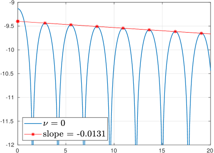
(a) $k=0.3,\nu=\nu_{\beta}=0$

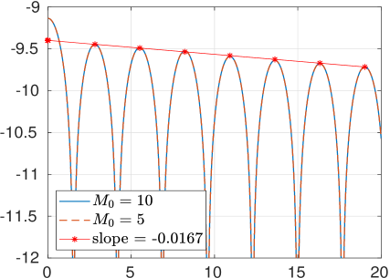
(b) $k=0.3,\nu=\nu_{\beta}=0.01$

Figure 1: Time evolution of $\ln(\mathcal{E}(t))$ with $N=800$ and $M=20$ for different $\nu$ in the linear Landau damping problem. The wave number $k=0.3$. For the collisional case, the red dashed line corresponds to $M_{0}=5$ while the blue line corresponds to $M_{0}=10$.

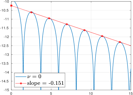
(a) $k=0.5,\nu=\nu_{\beta}=0$

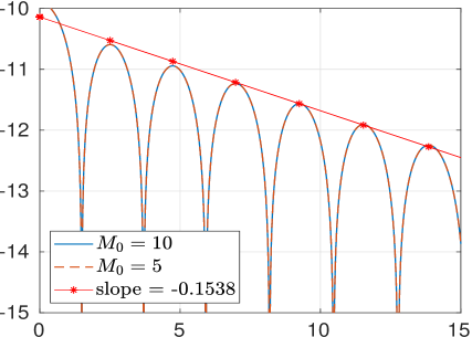
(b) $k=0.5,\nu=\nu_{\beta}=0.01$

Figure 2: Time evolution of $\ln(\mathcal{E}(t))$ with $N=800$ and $M=20$ for different $\nu$ in the linear Landau damping problem. The wave number $k=0.5$. For the collisional case, the red dashed line corresponds to $M_{0}=5$ while the blue line corresponds to $M_{0}=10$.

Then, we test the effect of different IPL models on our numerical method. The time evolution of the electrostatic energy $\mathcal{E}(t)$ for different potential indices $\gamma$, the index in the IPL model (2.7) aforementioned, is tested. Specifically, the model of Maxwell molecules $\gamma=0$ and the model with Coulomb interactions $\gamma=-3$ are tested and compared in Figure 3. Here, we also set the collisional frequency $\nu$ as $0.01$ and the wave number $k$ as $0.3$ and $0.5$, respectively. The numerical result illustrates that our method is capable of simulating the linear Landau damping for different $\gamma$, and we can conclude that the collision model with softer potential imposes a smaller damping rate.

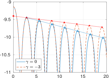
(a) $k=0.3,\nu=\nu_{\beta}=0.01$

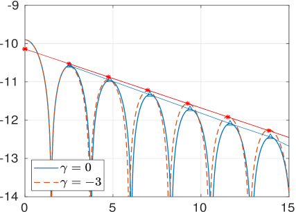
(b) $k=0.5,\nu=\nu_{\beta}=0.01$

Figure 3: Time evolution of $\ln(\mathcal{E}(t))$ with $N=800$ and $M_{0}=5$ for different $\gamma$ in the linear Landau damping problem. The blue line corresponds to $\gamma=0$ while the red dashed line corresponds to $\gamma=-3$.

6.2 Nonlinear Landau damping

As shown in the last section, when the wave amplitude $A$ is sufficiently small, the linear regime is valid, which yields exponentially decreasing electrostatic energy. However, the Landau damping problem with larger amplitude, which diverges from the linear theory and hence is also known as nonlinear Landau damping, is quite a different case. Typically, one finds that the amplitude decays, grows and oscillates before settling down to a relatively steady state [10].

In this section, we study the nonlinear Landau damping problem numerically. The nonlinear Landau damping is primarily attributed to the “trapping” phenomenon, where a particle is caught in the potential well of a wave, shuttles back and forth, and ends up gaining and losing energy to the wave [10].

In this numerical experiment, the form of the initial data is the same as that in the last section, with $A$ augmented to $0.2$ and the electrostatic energy is again studied. The nonlinear Landau damping problem with this particular initial data was also studied in [12, 53], to which we refer readers for a comparison of the numerical results. The case of Maxwell molecules $\gamma=0$ is studied, and the spatial grid size, expansion order and quadratic length are set as $N=800$, $M=20$ and $M_{0}=5$, respectively. Moreover, to avoid recurrence [17], the expansion order is chosen as $M=200$ for the collisionless case.

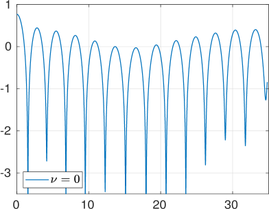
(a) $k=0.3,\nu=\nu_{\beta}=0$

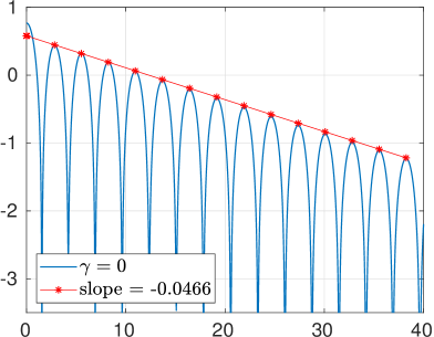
(b) $k=0.3,\nu=\nu_{\beta}=0.01$

(c) $k=0.3,\nu=\nu_{\beta}=0.05$

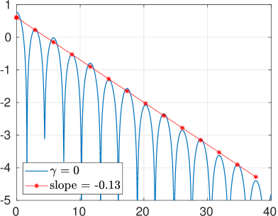
(d) $k=0.3,\nu=\nu_{\beta}=0.1$

Figure 4: Time evolution of $\ln(\mathcal{E}(t))$ with $N=800$ and $M_{0}=5$ for different collisional frequencies $\nu=\nu_{\beta}=0,0.01,0.05$ and $0.1$ in the nonlinear Landau damping problem. The wave number $k=0.3$.

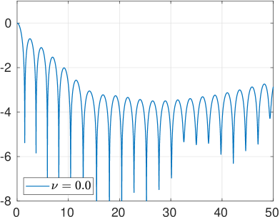
(a) $k=0.5,\nu=\nu_{\beta}=0$

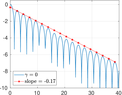
(b) $k=0.5,\nu=\nu_{\beta}=0.01$

(c) $k=0.5,\nu=\nu_{\beta}=0.05$

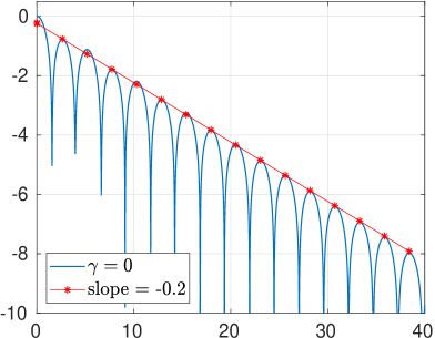
(d) $k=0.5,\nu=\nu_{\beta}=0.1$

Figure 5: Time evolution of $\ln(\mathcal{E}(t))$ with $N=800$ and $M_{0}=5$ for different collisional frequencies $\nu=\nu_{\beta}=0,0.01,0.05$ and $0.1$ in the nonlinear Landau damping problem. The wave number $k=0.5$.

Figures 4 and 5 show the time evolution of electrostatic energy for $k=0.3$ and $k=0.5$ with collisional frequency $\nu=\nu_{\beta}=0,0.01,0.05$ and $0.1$. We can conclude that for the nonlinear collisionless problem, instead of exponential damping as in the linear case, the electrostatic energy decreases exponentially at the beginning and then grows exponentially at a smaller rate, which is consistent with the results achieved by [11, 53]. For the collisional case, we find that the electrostatic energy exhibits an exponential-like damping for both wave numbers $k=0.3$ and $0.5$ and the damping rate increases with the collisional frequency. These results are reasonable because stronger collision implies more frequent energy exchange between particles and results in less “trapping” phenomena and faster damping rates. This numerical result also accords with that in [53, 12].

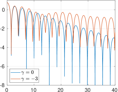
(a) $k=0.3,\nu=\nu_{\beta}=0.05$

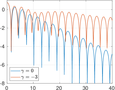
(b) $k=0.3,\nu=\nu_{\beta}=0.1$

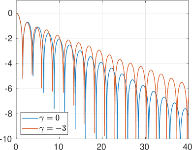
(c) $k=0.5,\nu=\nu_{\beta}=0.05$

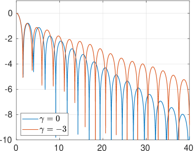
(d) $k=0.5,\nu=\nu_{\beta}=0.1$

Figure 6: Time evolution of $\ln(\mathcal{E}(t))$ with $N=800$ and $M_{0}=5$ for different potential indices $\gamma$ in the nonlinear Landau damping problem, where the blue line represents $\gamma=0$ and red line represents $\gamma=-3$. The first row corresponds to the wave number $k=0.3$ and the bottom row corresponds to the wave number $k=0.5$.

The cases of different potential indices in the IPL model are also studied, where the model of Maxwell molecules $\gamma=0$ and the model with Coulomb interactions $\gamma=-3$ are tested. Figure 6 shows the time evolution of the electrostatic energy for wave number $k=0.3$ and $0.5$ under different collisional frequencies $\nu=\nu_{\beta}=0.05$ and $0.1$, from which we find that the damping rate for the Maxwell case $\gamma=0$ is much larger than that for the Coulomb case $\gamma=-3$. This result is compatible with a similar conclusion in the linear case.

6.3 Two-stream instability

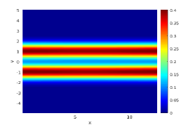
(a) Initial MDF $g(0,x,v_{1})$

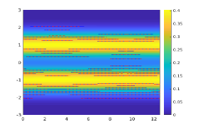
(b) Contours of $g(0,x,v_{1})$

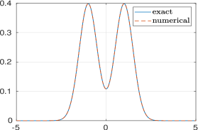
(c) Initial MDF $g(0,\frac{\pi}{4},v_{1})$

Figure 7: Initial marginal distribution functions of the two-stream instability problem. In (b) and (c), the blue solid lines correspond to the exact solution, and the red dashed lines correspond to the numerical approximation. Figure (a) shows only the numerical approximation. Figure (c) shows the numerical approximation and the exact solution at the position $x=\frac{\pi}{4}$.

Two-stream instability is a common instability in plasma physics and of primary concern for studying the nonlinear effect of plasma in the future. It occurs when the fluid consists of two electron streams with different velocities. The mechanism of two-stream instability is similar to that of Landau damping, where particles at different velocities transfer energy to each other [3].

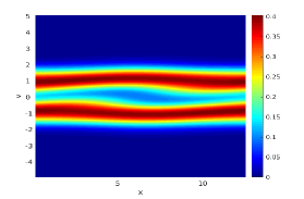
(a) $t=20,\nu=0$

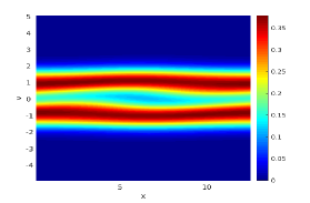
(b) $t=20,\nu=0.001$

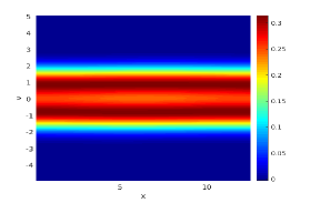
(c) $t=20,\nu=0.01$

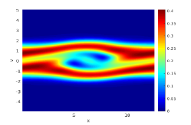
(d) $t=30,\nu=0$

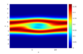
(e) $t=30,\nu=0.001$

(f) $t=30,\nu=0.01$

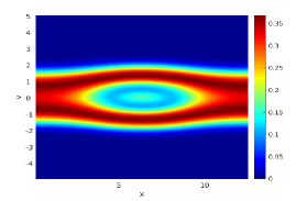
(g) $t=50,\nu=0$

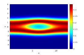
(h) $t=50,\nu=0.001$

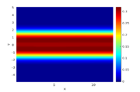
(i) $t=50,\nu=0.01$

Figure 8: Evolution of the marginal distribution function $g(t,x,v_{1})$ under different collisional frequencies $\nu$ in the two-stream instability problem. The left column corresponds to $\nu=0$, the middle column corresponds to $\nu=0.001$, and the right column corresponds to $\nu=0.01$.

In this numerical experiment, the initial data is given with a nonisotropic two-stream flow

$$f=\frac{(1+A\cos(kx))}{\sqrt{2\pi T}}\left[0.5\exp\left(-\frac{\left|\bm{v}-(u_{1},0,0)^{T}\right|^{2}}{2T}\right)+0.5\exp\left(-\frac{\left|\bm{v}+(u_{1},0,0)^{T}\right|^{2}}{2T}\right)\right],$$ (6.6)

with $A=0.01$, $T=0.25$ and $u_{1}=1$. Here, only the electron-electron collsion is considered and thus the electron-ion collision frequency $\nu_{\beta}$ is set as $0$. Similar initial data and assumptions can be found in [53]. The time evolution of the particles with the collisional model of Coulomb interactions $\gamma=-3$ is studied, and the wave number $k$ is chosen as $k=0.5$. The grid size and expansion order are chosen as $N=400$ and $M=40$, respectively. Moreover, the quadratic length is set as $M_{0}=5$. Here, the collisional frequency is set as $\nu=0$, $0.001$ and $0.01$ to present the effect of the collision. The marginal distribution function

$$g(t,x,v_{1})=\int_{\mathbb{R}^{2}}f(t,x,v_{1},v_{2},v_{3})\,\mathrm{d}v_{2}\,\mathrm{d}v_{3}$$ (6.7)

is also plotted to show the electron “trapping” phenomenon. Clearly, our chosen parameters can approximate the initial distribution function satisfactorily (see Figure 7). To suppress the recurrence and the nonphysical oscillations, the filter developed in [28, 17] is applied here.

Figure 8 shows the time evolution of the marginal distribution function (6.7) in the $x-v_{1}$ plane. From these, we can find that for the collisionless case, the linear two-stream instability grows exponentially at first, and then the nonlinearity becomes dominant and “trapping” emerges. At the same time, the original distribution begins to twist and curve until an electron hole-like structure finally forms, which is consistent with the results in [26]. For the collisional case, a smaller electron hole-like structure forms with the increase in the collisional frequency $\nu$, and no visible hole-like structure occurs in the case of collisional frequency $\nu=0.1$. This again substantiates the effect of collision to reduce the “trapping” phenomenon.

The time evolution of the total energy is also studied to test the conservation property of this numerical scheme. The total energy $\mathcal{E}_{t}(t)$ is defined as

$$\mathcal{E}_{t}(t)=\frac{1}{2}\Delta x\sum_{j}\int_{\mathbb{R}^{3}}f(t,x_{j},\bm{v})|\bm{v}|^{2}\,\mathrm{d}\bm{v}+\frac{1}{2}\mathcal{E}(t)^{2}.$$ (6.8)

The evolution of the total energy $\mathcal{E}_{t}(t)$ for different collisional frequencies is plotted in Figure 9, from which we can see that although the numerical scheme cannot exactly preserve the total energy, the variation of the total energy is minute, especially in the linear instability stage, where the variation is almost negligible.

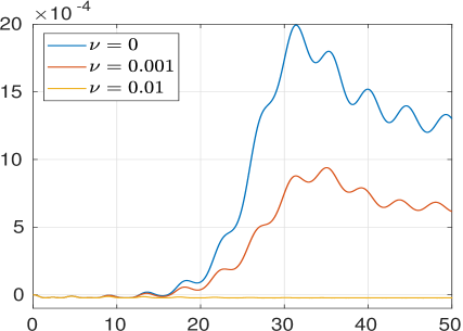
Figure 9: Time evolution of the variation in the total energy $\mathcal{E}_{t}(t)$ for different collisional frequencies in the two-stream instability problem. The variation is defined as $(\mathcal{E}_{t}(t)-\mathcal{E}_{t}(0))/\mathcal{E}_{t}(0)$.

6.4 Bump-on-tail instability

Bump-on-tail instability is another important micro-instability which is a special case of two-stream instability when the two electron streams have different densities [11]. The distribution function is unstable, which leads to growth in the initial perturbation followed by saturation and oscillation of the particles trapped in the potential through the wave [43, 46].

In this numerical experiment, we also begin with a nonisotropic distribution function as

$$f=\frac{(1+A\sin(kx))}{\sqrt{2\pi T}}\left[n_{m}\exp\left(-\frac{\left|\bm{v}-(u_{1},0,0)^{T}\right|^{2}}{2T}\right)+n_{b}\exp\left(-\frac{\left|\bm{v}+(u_{1},0,0)^{T}\right|^{2}}{2T}\right)\right],$$ (6.9)

where $A=0.01$, $T=0.25$ and $u_{1}=1$. $n_{m}=0.7$, which represents the magnitude of the “mainstream”, and $n_{b}=0.3$, representing the magnitude of the “bump” on the tail of the “mainstream”.

The wave number $k$ is chosen as $k=0.3$. The grid size is chosen as $N=400$, and the expansion order is set as $M=40$, which gives a satisfying approximation to the initial distribution function (see Figure 10). Moreover, the quadratic length is set as $M_{0}=5$. Similar to the previous numerical experiment, we focus on the model with Coulomb interactions, and the time evolution of particles with collision frequencies $\nu=0$, $0.001$ and $0.01$ is studied.

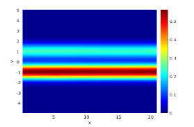
(a) Initial MDF $g(0,x,v_{1})$

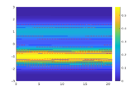
(b) Contours of $g(0,x,v_{1})$

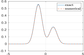
(c) Initial MDF $g(0,0,v_{1})$

Figure 10: Initial marginal distribution functions of the bump-on-tail instability problem. In (b) and (c), the blue solid lines correspond to the exact solution, and the red dashed lines correspond to the numerical approximation. Figure (a) shows only the numerical approximation. Figure (c) shows the numerical approximation and the exact solution at the position $x=0$.

Figure 11 shows the time evolution of the marginal distribution function (6.7) in the $x-v_{1}$ plane. We can observe that for the collisionless case, the bump is trapped by the electric field and gradually forms a crawling vortex-like structure. For the collisional case, the trapping of the bump is much weaker, and the distribution of the “mainstream” is less affected. In the case of the collisional frequency $\nu=0.1$, no vortex-like structure is perceptible.

The evolution of the total energy defined in (6.8) is also studied. Figure 12 shows the evolution of the total energy for different collisional frequencies. Although the total energy is not perfectly preserved, the variation in the total energy is small, especially at the beginning of the evolution and decreases with the increase in the collisional frequency.

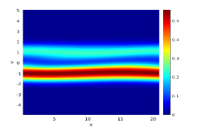
(a) $t=20,\nu=0.0$

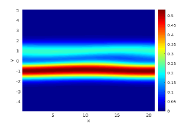
(b) $t=20,\nu=0.001$

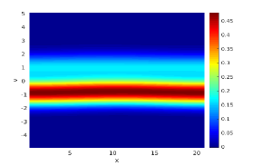
(c) $t=20,\nu=0.01$

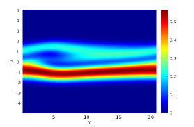
(d) $t=30,\nu=0.0$

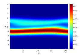
(e) $t=30,\nu=0.001$

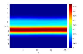
(f) $t=30,\nu=0.01$

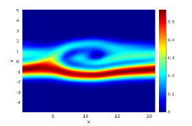
(g) $t=40,\nu=0.0$

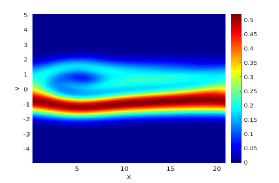
(h) $t=40,\nu=0.001$

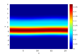
(i) $t=40,\nu=0.01$

Figure 11: Evolution of the marginal distribution function $g(t,x,v_{1})$ under different collisional frequencies $\nu$ in the bump-on-tail instability problem. The left column corresponds to $\nu=0$ , the middle column corresponds to $\nu=0.001$, and the right column corresponds to $\nu=0.01$.

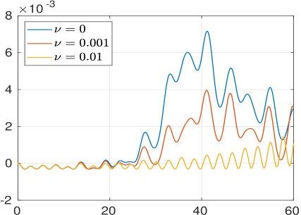
Figure 12: Time evolution of the variation in the total energy $\mathcal{E}_{t}(t)$ for different collisional frequencies in the bump-on-tail instability problem. The variation is defined as $(\mathcal{E}_{t}(t)-\mathcal{E}_{t}(0))/\mathcal{E}_{t}(0)$.

7 Conclusion

In this paper, we developed a numerical algorithm for the FPL equation based on the Hermite spectral method. Both collisions within the same species and between different species were considered to simulate the time evolution of plasma. A reduced collision model was built by combining the quadratic FPL collision operator and the diffusive FP collision operator. A fast algorithm to project between distribution functions with different expansion centers was adopted. Several numerical experiments showed that our numerical algorithm can capture the time evolution of the particles accurately and efficiently compared to the fully quadratic collision model.

The effect of the new reduced collision operator makes this algorithm promising when dealing with more complicated problems. However, this method is not capable of dealing with the problems that the state of the plasma diverges greatly from equilibrium, which we will work on in the future. Research on multidimensional problems with the magnetic field is also ongoing.

8 Appendix

In this section, we introduce a detailed calculation of the expansion coefficients for the collision operator (2.14) in Section 8.1 and the derivation of the governing equations (5.3) for the acceleration step in Section 8.2.

8.1 Calculation of the expansion coefficient (4.13)

In this section, we introduce a detailed calculation of the expansion coefficients in (4.13). Bringing the explicit form of the collision operator $\mathcal{Q}_{\beta}[f]$ in (2.14) into (4.12) and integrating by parts, the expansion coefficients $\mathcal{Q}_{\beta,\bm{i}}^{[\bm{u}_{\beta},1]}$ are calculated as

$$\mathcal{Q}_{\beta,\bm{i}}^{[\bm{u}_{\beta},1]}(t,\bm{x}) =-\frac{1}{\bm{i}!}\int_{\mathbb{R}^{3}}\left[{\bf A}(\bm{v}-\bm{u}_{\beta})\nabla_{\bm{v}}f\right]\cdot\nabla_{\bm{v}}H_{\bm{i}}\left(\bm{v}-\bm{u}_{\beta}\right)\,\mathrm{d}\bm{v}.$$ (8.1)

Expanding the distribution function $f$ as

$$f(t,\bm{x},\bm{v})\approx\sum_{\bm{j}\in\mathbb{N}^{3}}f_{\bm{j}}^{[\bm{u}_{\beta},1]}(t,\bm{x})\mathcal{H}_{\bm{j}}^{[\bm{u}_{\beta},1]},$$ (8.2)

we can calculate (8.1) as

$$\mathcal{Q}_{\beta,\bm{i}}^{[\bm{u}_{\beta},1]}(t,\bm{x}) =-\frac{1}{\bm{i}!}\sum_{\bm{j}\in\mathbb{N}^{3}}f_{\bm{j}}^{[\bm{u}_{\beta},1]}(t,\bm{x})C_{\bm{i}}^{\bm{j}},$$ (8.3)

with

$$C_{\bm{i}}^{\bm{j}} =\int_{\mathbb{R}^{3}}\left[{\bf A}(\bm{v}-\bm{u}_{\beta})\nabla_{\bm{v}}\mathcal{H}_{\bm{j}}^{[\bm{u}_{\beta},1]}(\bm{v})\right]\cdot\nabla_{\bm{v}}H_{\bm{i}}\left(\bm{v}-\bm{u}_{\beta}\right)\,\mathrm{d}\bm{v}.$$ (8.4)

By changing variables and utilizing the differentiation property of the basis function (4.8), we can derive

$$C_{\bm{i}}^{\bm{j}}=-\sum_{m,n=1}^{3}\int_{\mathbb{R}^{3}}\left[{\bf A}(\bm{v})\right]_{mn}\mathcal{H}_{\bm{j}+\bm{e}_{n}}^{[\bm{0},1]}(\bm{v})i_{m}H_{\bm{i}-\bm{e}_{m}}\left(\bm{v}\right)\,\mathrm{d}\bm{v}.$$ (8.5)

Recalling the definition of ${\bf A}(\bm{v}-\bm{u}_{\beta})$ in (2.6), we expand (8.5) as

$$C_{\bm{i}}^{\bm{j}}=\Lambda\sum_{m,n=1}^{3}i_{m}\Big{[}\int_{\mathbb{R}^{3}}\delta_{mn}\sum_{s=1}^{3}|\bm{v}|^{\gamma}v_{s}^{2}\mathcal{H}_{\bm{j}+\bm{e}_{n}}^{[\bm{0},1]}(\bm{v})H_{\bm{i}-\bm{e}_{m}}\,\mathrm{d}\bm{v}-\int_{\mathbb{R}^{3}}|\bm{v}|^{\gamma}v_{m}v_{n}\mathcal{H}_{\bm{j}+\bm{e}_{n}}^{[\bm{0},1]}(\bm{v})i_{m}H_{\bm{i}-\bm{e}_{m}}\left(\bm{v}\right)\,\mathrm{d}\bm{v}\Big{]}.$$ (8.6)

Finally, with the definition in [36, Eq.(3.14)], i.e.

$$G_{mn}\big{(}\gamma,\bm{i},\bm{j}\big{)}=\int_{\mathbb{R}^{3}}|\bm{v}|^{\gamma}v_{m}v_{n}H_{\bm{i}}\left(\bm{v}\right)H_{\bm{j}}(\bm{v})\dfrac{1}{(2\pi)^{3/2}}\exp{\left(-\dfrac{|\bm{v}|^{2}}{2}\right)}\,\mathrm{d}\bm{v},$$ (8.7)

we can derive the final expression of the expansion coefficients (4.13).

8.2 Deduction of the governing equation in the acceleration step

In this section, we present the deduction of the governing equation (5.3) in the acceleration step with the expansion center $\tilde{\bm{u}}=\bm{u}$ and $\tilde{T}=T$. A similar deduction can be found in [8], to which we refer readers for more details. In this case, the distribution function $f$ is expanded as

$$f(t,\bm{x},\bm{v})=\sum_{\bm{i}\in\mathbb{N}^{3}}f_{\bm{i}}^{[\bm{u},T]}(t,\bm{x})\mathcal{H}_{\bm{i}}^{[\bm{u},T]}(\bm{v}).$$ (8.8)

Substituting (8.8) into the FPL equation (2.2), we can derive the moment equations with some rearrangement as

$$\begin{split}&\frac{\partial f_{\bm{i}}}{\partial t}+\sum_{d=1}^{3}\left(\frac{\partial u_{d}}{\partial t}+\sum_{j=1}^{3}u_{j}\frac{\partial u_{d}}{\partial x_{j}}-F_{d}\right)f_{\bm{i}-\bm{e}_{d}}\\ &+\sum_{j,d=1}^{3}\left[\frac{\partial u_{d}}{\partial x_{j}}\left(Tf_{\bm{i}-\bm{e}_{d}-\bm{e}_{j}}+(i_{j}+1)f_{\bm{i}-\bm{e}_{d}+\bm{e}_{j}}\right)+\frac{1}{2}\frac{\partial T}{\partial x_{j}}\left(Tf_{\bm{i}-2\bm{e}_{d}-\bm{e}_{j}}+(i_{j}+1)f_{\bm{i}-2\bm{e}_{d}+\bm{e}_{j}}\right)\right]\\ &+\frac{1}{2}\left(\frac{\partial T}{\partial t}+\sum_{j=1}^{3}u_{j}\frac{\partial T}{\partial x_{j}}\right)\sum_{d=1}^{3}f_{\bm{i}-2\bm{e}_{d}}+\sum_{j=1}^{3}\left(T\frac{\partial f_{\bm{i}-\bm{e}_{j}}}{\partial x_{j}}+u_{j}\frac{\partial f_{\bm{i}}}{\partial x_{j}}+(i_{j}+1)\frac{\partial f_{\bm{i}+\bm{e}_{j}}}{\partial x_{j}}\right)=Q_{\bm{i}},\end{split}$$ (8.9)

where $[\bm{u},T]$ are omitted and $Q_{\bm{i}}$ is the expansion for the collision term. Following the method in [7], we deduce the mass conservation in the case of $\bm{i}=\bm{0}$ as

$$\frac{\partial f_{\bm{0}}}{\partial x_{j}}+\sum_{j=1}^{3}\left(u_{j}\frac{\partial f_{\bm{0}}}{\partial x_{j}}+f_{\bm{0}}\frac{\partial u_{j}}{\partial x_{j}}\right)=0.$$ (8.10)

If we set $\bm{i}=\bm{e}_{d}$, with $d=1,2,3$, (8.9) reduces to

$$f_{\bm{0}}\left(\frac{\partial u_{d}}{\partial t}+\sum_{j=1}^{3}u_{j}\frac{\partial u_{d}}{\partial x_{j}}-F_{d}\right)+f_{\bm{0}}\frac{\partial T}{\partial x_{d}}+T\frac{\partial f_{\bm{0}}}{\partial x_{d}}+\sum_{j=1}^{3}(\delta_{jd}+1)\frac{\partial f_{\bm{e}_{d}+\bm{e}_{j}}}{\partial x_{j}}=0.$$ (8.11)

With the splitting method stated in Section 5, (8.11) is split into the convection step

$$f_{\bm{0}}\left(\frac{\partial u_{d}}{\partial t}+\sum_{j=1}^{3}u_{j}\frac{\partial u_{d}}{\partial x_{j}}\right)+f_{\bm{0}}\frac{\partial T}{\partial x_{d}}+T\frac{\partial f_{\bm{0}}}{\partial x_{d}}+\sum_{j=1}^{3}(\delta_{jd}+1)\frac{\partial f_{\bm{e}_{d}+\bm{e}_{j}}}{\partial x_{j}}=0,$$ (8.12)

and the force step

$$\dfrac{\partial{u_{d}}}{\partial{t}}-F_{d}=0,\qquad d=1,2,3.$$ (8.13)

Then, we obtain the governing equations (5.3) for the acceleration step.

References

- [1] Y. Berezin, V. Khudick, and M. Pekker. Conservative finite-difference schemes for the Fokker-Planck equation not violating the law of an increasing entropy. J. Comput. Phys., 69(1):163–174, 1987.
- [2] G. Bird. Molecular Gas Dynamics and the Direct Simulation of Gas Flows. Oxford: Clarendon Press, 1994.
- [3] J. Bittencourt. Fundamentals of plasma physics. Springer Science & Business Media, 2013.
- [4] S. Bourdiec, F. Vuyst, and L. Jacquet. Numerical solution of the Vlasov-Poisson system using generalized Hermite functions. Commun. Comput. Phys., 175(8):528–544, 2006.
- [5] C. Buet and S. Cordier. Conservative and entropy decaying numerical scheme for the isotropic Fokker-Planck-Landau equation. J. Comput. Phys., 145(1):1228–245, 1998.
- [6] C. Buet, S. Cordier, P. Degond, and M. Lemou. Fast algorithms for numerical, conservative, and entropy approximations of the Fokker-Planck-Landau equation. J. Comput. Phys., 133(2):310 – 322, 1997.
- [7] Z. Cai, R. Li, and Z. Qiao. NR simulation of microflows with Shakhov model. SIAM J. Sci. Comput., 34(1):A339–A369, 2012.
- [8] Z. Cai, R. Li, and Y. Wang. Solving Vlasov equation using NR method. SIAM J. Sci. Comput., 35(6):A2807–A2831, 2013.
- [9] J. Chang and G. Cooper. A practical difference scheme for Fokker-Planck equations. J. Comput. Phys., 6:1–16, 1970.
- [10] F. Chen. Introduction to plasma physics and controlled fusion, volume 1. Springer, 1984.
- [11] Y. Cheng, A. Christlieb, and X. Zhong. Energy-conserving discontinuous Galerkin methods for the Vlasov-Ampére system. J. Comput. Phys., 256:630–665, 2014.
- [12] N. Crouseilles and F. Filbet. Numerical approximation of collisional plasmas by high order methods. J. Comput. Phys., 201(2):546–572, 2004.
- [13] N. Crouseilles, M. Mehrenberger, and E. Sonnendrücker. Conservative semi-Lagrangian schemes for Vlasov equations. J. Comput. Phys., 229(6):1927 – 1953, 2010.
- [14] P. Degond and B. Lucquin-Desreux. The Fokker-Planck asymptotics of the Boltzmann collision operator in the coulomb case. Math. Models Meth. Appl. Sci., 02(02):167–182, 1992.
- [15] P. Degond and B. Lucquin-Desreux. An entropy scheme for the Fokker-Planck collision operator of plasma kinetic theory. Numer. Math., 68:239–262, 1994.
- [16] L. Desvillettes. On asymptotics of the Boltzmann equation when the collisions become grazing. Transport. Theor. Stat., 21(3):259–276, 1992.
- [17] Y. Di, Y. Fan, Z. Kou, R. Li, and Y. Wang. Filtered hyperbolic moment method for the Vlasov equation. J. Sci. Comput., 79(2):969–991, 2019.
- [18] G. Dimarco, Q. Li, L. Pareschi, and B. Yan. Numerical methods for plasma physics in collisional regimes. J. Plasma Phys., 81(1):305810106, 2015.
- [19] F. Filbet and S. Jin. A class of asymptotic preserving schemes for kinetic equations and related problems with stiff sources. J. Comput. Phys., 229:7625–7648, 2010.
- [20] F. Filbet and L. Pareschi. A numerical method for the accurate solution of the Fokker-Planck-Landau equation in the nonhomogeneous case. J. Comput. Phys., 179(1):1–26, 2002.
- [21] F. Filbet and E. Sonnendrücker. Numerical methods for the Vlasov equation. In Numerical Mathematics and Advanced Applications, pages 459–468, Milano, 2003. Springer Milan.
- [22] F. Filbet and T. Xiong. Conservative discontinuous Galerkin/Hermite spectral method for the Vlasov-Poisson system. Commun. Appl. Math. Comput., 2020.
- [23] J. Fok, B. Guo, and T. Tang. Combined Hermite spectral-finite difference method for the Fokker-Planck equation. Math. Comp., 71:1497–1528, 2002.
- [24] L. Gibelli and B. Shizgal. Spectral convergence of the Hermite basis function solution of the Vlasov equation: The free-streaming term. J. Comput. Phys., 219(2):477–488, 2006.
- [25] T. Goudon. On Boltzmann equations and Fokker-Planck asymptotics: Influence of grazing collisions. J. Stat. Phts., 89:751, 1997.
- [26] R. Heath, I. Gamba, P. Morrison, and C. Michler. A discontinuous Galerkin method for the Vlasov-Poisson system. J. Comput. Phys., 231(4):1140–1174, 2012.
- [27] J. Holloway. Spectral velocity discretizations for the Vlasov-Maxwell equations. Transport Theor. Stat., 25(1):1–32, 1996.
- [28] T. Hou and R. Li. Computing nearly singular solutions using pseudo-spectral methods. J. Comput. Phys., 226(1):379–397, 2007.
- [29] Z. Hu, Z. Cai, and Y. Wang. Numerical simulation of microflows using Hermite spectral methods. SIAM J. Sci. Comput., 42(1):B105–B134, 2020.
- [30] S. Jin and B. Yan. A class of asymptotic-preserving schemes for the Fokker-Planck-Landau equation. J. Comput. Phys., 230:6420–6437, 2011.
- [31] T. Kho. Relaxation of a system of charged particles. Phys. Rev. A, 32(1):666–669, 1985.
- [32] L. Landau. Kinetic equation for the case of Coulomb interaction. Phys. Zs. Sov. Union, 10:154–164, 1936.
- [33] M. Lemou. Multipole expansions for the Fokker-Planck-Landau operator. Numer. Math., 78(4):597–618, Feb 1998.
- [34] M. Lemou and L. Mieussens. Implicit schemes for the Fokker-Planck-Landau equation. SIAM J. Sci. Comput., 27(3):809–830, 2005.
- [35] R. LeVeque. Finite Volume Methods for Hyperbolic Problems. Cambridge, 2002.
- [36] R. Li, Y. Wang, and Y. Wang. Approximation to singular quadratic collision model in Fokker-Planck-Landau equation. SIAM J. Sci. Comput., 42(3):B792–B815, 2020.
- [37] K. Nanbu and S. Yonemura. Weighted particles in Coulomb collision simulations based on the theory of a cumulative scattering angle. J. Comput. Phys., 145(2):639 – 654, 1998.
- [38] L. Pareschi, G. Russo, and G. Toscani. Fast spectral methods for the Fokker-Planck-Landau collision operator. J. Comput. Phys., 165(1):216 – 236, 2000.
- [39] J. Parker and P. Dellar. Fourier–Hermite spectral representation for the Vlasov–Poisson system in the weakly collisional limit. J. Plasma Phys., 81(02):305810203, 2015.
- [40] J. Qiu and C. Shu. Positivity preserving semi-Lagrangian discontinuous Galerkin formulation: Theoretical analysis and application to the Vlasov-Poisson system. J. Comput. Phys., 230(23):8386 – 8409, 2011.
- [41] M. Rosenbluth, W. MacDonald, and D. Judd. Fokker-Planck equation for an inverse-square force. Phys. Rev., 107:1–6, Jul 1957.
- [42] J. Schumer and J. Holloway. Vlasov simulation using velocity-scaled Hermite representations. J. Comput. Phys., 144(2):626–661, 1998.
- [43] M. Shoucri. Nonlinear evolution of the bump-on-tail instability. Phys. Fluids, 22(10):2038–2039, 1979.
- [44] E. Sonnendrücker, J. Roche, P. Bertrand, and A. Ghizzo. The semi-Lagrangian method for the numerical resolution of the Vlasov equation. J. Comput. Phys., 149(2):201–220, 1999.
- [45] W. Taitano, L. Chacón, A. Simakov, and K. Molvig. A mass, momentum, and energy conserving, fully implicit, scalable algorithm for the multi-dimensional, multi-species Rosenbluth-Fokker-Planck equation. J. Comput. Phys., 297:357 – 380, 2015.
- [46] N. Takashi and Y. Takashi. Cubic interpolated propagation scheme for solving the hyper-dimensional Vlasov-Poisson equation in phase space. Comput. Phys. Commun., 120(2):122 – 154, 1999.
- [47] C. Villani. On the spatially homogeneous Landau equation for Maxwellian molecule. Math. Models Methods Appl. Sci., 08(06):957–983, 1998.
- [48] Y. Wang and S. Zhang. Solving Vlasov-Poisson-Fokker-Planck equations using NR method. Commun. Comput. Phys., 21(3):782–807, 2017.
- [49] T. Xiong, J. Qiu, Z. Xu, and A. Christlieb. High order maximum principle preserving semi-Lagrangian finite difference WENO schemes for the Vlasov equation. J. Comput. Phys., 273(273):618–639, 2014.
- [50] E. Yoon and C. Chang. A Fokker-Planck-Landau collision equation solver on two-dimensional velocity grid and its application to particle-in-cell simulation. Phys. Plasmas, 21:032503, 2014.
- [51] S. Zaki, T. Boyd, and L. Gardner. A finite element code for the simulation of one-dimensional Vlasov plasmas. ii. applications. J. Comput. Phys., 79(1):200–208, 1988.
- [52] S. Zaki, L. Gardner, and T. Boyd. A finite element code for the simulation of one-dimensional Vlasov plasmas. i. theory. J. Comput. Phys., 79(1):184 –199, 1988.
- [53] C. Zhang and I. Gamba. A conservative scheme for Vlasov Poisson Landau modeling collisional plasmas. J. Comput. Phys., 340:470–497, 2017.