Faster Stochastic Quasi-Newton Methods

Abstract

Stochastic optimization methods have become a class of popular optimization tools in machine learning. Especially, stochastic gradient descent (SGD) has been widely used for machine learning problems such as training neural networks due to low per-iteration computational complexity. In fact, the Newton or quasi-newton methods leveraging second-order information are able to achieve better solution than the first-order methods. Thus, stochastic quasi-Newton (SQN) methods have been developed to achieve better solution efficiently than the stochastic first-order methods by utilizing approximate second-order information. However, the existing SQN methods still do not reach the best known stochastic first-order oracle (SFO) complexity. To fill this gap, we propose a novel faster stochastic quasi-Newton method (SpiderSQN) based on the variance reduced technique of SIPDER. We prove that our SpiderSQN method reaches the best known SFO complexity of $\mathcal{O}(n+n^{1/2}\epsilon^{-2})$ in the finite-sum setting to obtain an $\epsilon$-first-order stationary point. To further improve its practical performance, we incorporate SpiderSQN with different momentum schemes. Moreover, the proposed algorithms are generalized to the online setting, and the corresponding SFO complexity of $\mathcal{O}(\epsilon^{-3})$ is developed, which also matches the existing best result. Extensive experiments on benchmark datasets demonstrate that our new algorithms outperform state-of-the-art approaches for nonconvex optimization.

Keywords: Stochastic quasi-Newton method, nonconvex optimization, variance reduction, momentum acceleration

1 Introduction

In this paper, we focus on the following unconstrained stochastic nonconvex optimization: where $x\in\mathbb{R}^{d}$ corresponds to the parameters defining a model, ${\mathbb{E}_{u\sim\mathbb{P}}[f_{u}(x)]}$ denotes a population risk over $u\sim\mathbb{P}$, and $f_{i}:\mathbb{R}^{d}\to\mathbb{R}$ denotes the loss on the $i$-th sample for $\forall\ i\in{1,...,n}$ (or $i\sim\mathbb{P}$). Problem (LABEL:eq:_P) capsules a widely range of machine learning problems such as truncated square loss Xu et al. (2018) for regression and deep neural network Goodfellow et al. (2016). In fact, the SGD Ghadimi et al. (2016) is a representative method to solve the problem (LABEL:eq:_P) due to its per-iteration computation efficiency. Recently, there have been many works studying SGD and its variance reduction variants, including SVRG Reddi et al. (2016a), SAGA Reddi et al. (2016b), SCSGLei et al. (2017), SARAH Nguyen et al. (2017b), SNVRG Zhou et al. (2018a) and SPIDER Fang et al. (2018); Wang et al. (2019). In particular, SPIDER has been shown in Fang et al. (2018) to achieve the SFO complexity lower bound for a certain regime. Such idea has been extended to optimization over mainfolds in Zhou et al. (2019b), zeroth-order optimization in Huang et al. ; Ji et al. (2019), cubic-regularized method in Zhou and Gu (2020), and alternating direction method of multipliers in Huang et al. (2019).

Although SGD is very effective, its performance maybe poor owing that it only utilizes the first-order information. In contrast, Newton’s method utilizing the Hessian information is more robust and can achieve better accuracy Sohl-Dickstein et al. (2014); Allen-Zhu (2018), while it is extremely time consuming to compute Hessian matrix and its inverse. Therefore, many works have been proposed toward designing better SGD methods integrated with approximate Hessian information, i.e., the SQN methods. There have been many works focusing on developing SQN methods such as SGD with quasi-Newton (SGD-QN) studied in Bordes et al. (2009) and stochastic approximation based L-BFGS proposed in Byrd et al. (2016). Recently, some SQN methods equipped with the variance reduction technique have been developed to alleviate the effect of variance introduced by stochastic estimator Kolte et al. (2015); Lucchi et al. (2015); Moritz et al. (2016); Gower et al. (2016). Besides above methods concerning convex or strongly convex problems, progresses have been made toward designing SQN methods for nonconvex cases. Wang et al. Wang et al. (2017) analyzed the convergence guarantee of the SGD-QN for nonconvex problems, Wang et al. Wang et al. (2018a) developed a stochastic proximal quasi-Newton for nonconvex composite optimization, and Gao et al. Gao and Huang (2018) proposed the stochastic L-BFGS method for nonconvex sparse learning problems.

Stochastic quasi-Newton methods inherit many appealing advantages from both SGD and quasi-Newton methods, e.g., efficiency, robustness and better accuracy. However, existing SQN methods still do not reach the best known SFO complexity, resulting the limited application to machine learning. It is thus of vital importance to improve the SFO complexity of SQN methods for nonconvex optimization. For this reason, we propose a faster SQN method (namely SpiderSQN) by leveraging the variance reduction technique of SIPDER.

Albeit SpiderSQN achieves the optimal SFO complexity for nonconvex optimization, its practical performance may not exhibit such optimality. Thus, we consider utilizing momentum acceleration technology to obtain better practical performance. Moreover, to deal with cases where the number of training samples is extremely large or even infinite, the SpiderSQN based algorithms are extended to the online case with theoretical guarantee. To give a thorough comparison of our proposed algorithm with existing stochastic first-order algorithms and SQN for nonconvex optimization, we summarize the SFO complexity of the most relevant algorithms to achieve an $\epsilon$-first-order stationary point in Table 1. The main contributions of this paper are summarized as follows.

1. We propose a novel faster stochastic quasi-Newton method (SpiderSQN) for nonconvex optimization in the form of finite-sum. Moreover, we prove that the SpiderSQN can achieve the best known optimal SFO complexity of $\mathcal{O}(n+n^{1/2}\epsilon^{-2})$ to obtain an $\epsilon$-first-order stationary point.

2. We extend the SpiderSQN to the online setting, and propose the faster online SpiderSQN algorithms for nonconvex optimization. Moreover, we prove that the online SpiderSQN achieve the best known optimal SFO complexity of $\mathcal{O}(\epsilon^{-3})$.

3. To improve the practical performance of the proposed methods, we apply momentum schemes to them, which are demonstrated to have satisfactory practical effects.

4. Moreover, we prove that our SpiderSQN methods have the lower SFO complexity of $\mathcal{O}(n^{1/2}\epsilon^{-1/2})$, which achieves the optimal SFO complexity of $\mathcal{O}(n^{1/2}\epsilon^{-1/2})$.

Table 1: Comparison of results on SFO complexity for smooth nonconvex optimization. Note that we omit the poly-logarithmic factors of $d,n,\epsilon$. Especially, SpiderSQN-M represents SpiderSQN with different momentum schemes.

Algorithm	Finite-sum	Online
SGD Ghadimi et al. (2016)	$\mathcal{O}({n\epsilon^{-2}})$	$\mathcal{O}({\epsilon^{-4}})$
SVRGReddi et al. (2016a)	$\mathcal{O}({n+n^{\frac{2}{3}}\epsilon^{-2}})$	$\mathcal{O}({\epsilon^{-\frac{10}{3}}})$
SARAH Nguyen et al. (2017b)	$\mathcal{O}({n+\epsilon^{-4}})$	$\mathcal{O}({\epsilon^{-4}})$
SNVRG Zhou et al. (2018a)	$\mathcal{O}({n+n^{\frac{1}{2}}\epsilon^{-2}})$	$\mathcal{O}({\epsilon^{-3}})$
SPIDER Fang et al. (2018); Wang et al. (2019)	$\mathcal{O}({n+n^{\frac{1}{2}}\epsilon^{-2}})$	$\mathcal{O}({\epsilon^{-3}})$
SQN with SGD Wang et al. (2017)	$\mathcal{O}({n\epsilon^{-2}})$	$N/A$
SQN with SVRG Wang et al. (2017)	$\mathcal{O}({n+n^{\frac{2}{3}}\epsilon^{-2}})$	$N/A$
SpiderSQN (Ours)	$\mathcal{O}({n+n^{\frac{1}{2}}\epsilon^{-2}})$	$\mathcal{O}({\epsilon^{-3}})$
SpiderSQN-M (Ours)	$\mathcal{O}({n+n^{\frac{1}{2}}\epsilon^{-2}})$	$\mathcal{O}({\epsilon^{-3}})$

2 Preliminaries

In this section, some preliminaries are presented. Since finding the global minimum of problem (LABEL:eq:_P) is general NP-hard Hillar and Lim (2013), this work instead focuses on finding an $\epsilon$-first-order stationary point and studies the SFO complexity of achieving it. First, we give the necessary definitions and assumptions.

Definition 1

An $\epsilon$-first-order stationary point denotes that for $x$ uniformly drawn from $x_{1},\cdots,x_{K}$, where $K$ is the total number of iterations there is $\mathbb{E}\|\nabla f(x)\|\leq\epsilon$, where $\epsilon>0$ is the accuracy parameter.

Definition 2

Given a sample $i$ ($i\in 1,\cdots,n$ or $i\sim\mathbb{P}$) and a point $x\in\mathbb{R}^{d}$, a stochastic/incremental first-order oracle (SFO/IFO) Reddi et al. (2016a) returns the pair $(f_{i}(x),\nabla f_{i}(x))$.

Assumption 1

Function $f$ is bounded below, i.e.,

$$f^{*}:=\inf_{x\in\mathbb{R}^{d}}f(x)>-\infty.$$ (11)

Assumption 2

Individual function $f_{i},i=1,\ldots,n$ or $i\sim\mathbb{P}$ is $L$-smooth, i.e., there exists an $L>0$ such that

$$\|\nabla f_{i}(x)-\nabla f_{i}(y)\|\leq L\|x-y\|,\quad\forall x,y\in\mathbb{R}^{d},$$ (12)

Above two assumptions are standard in the analysis of nonconvex optimization Ghadimi and Lan (2016); Huang et al. (2019, ), where Assumption 1 guarantees the feasibility of problem (LABEL:eq:_P) and Assumption 2 imposes smoothness on the individual loss functions.

Assumption 3

For $\forall i\in 1,\cdots,n$ (or $i\sim\mathbb{P}$), function $f_{i}(x)$ is twice continuously differentiable with respect to $x$. There exists a positive constant $\kappa$ such that $\|\nabla^{2}f_{i}(x)\|\leq\kappa$ for $\forall$ $x$.

Note that Assumption 3 is standard for SQN methods focusing on nonconvex problem Wang et al. (2017).

Assumption 4

There exist two positive constants $\sigma_{\mathrm{min}}$, and $\sigma_{\mathrm{max}}$ such that

$$\sigma_{\mathrm{min}}I\preceq H_{k}\preceq\sigma_{\mathrm{max}}I,$$ (13)

where $H_{k}$ is the inverse Hessian approximation matrix and notation $A\preceq B$ with $A,B\in\mathbb{R}^{d\times d}$ means that $A-B$ is positive semidefinite.

Assumption 5

For any $k\geq 2$, the random variable $H_{k}$ ($k\geq 2$) depends only on $v_{k-1}$ and $\xi_{k}$

$$\mathbb{E}[H_{k}v_{k}|\xi_{k},v_{k-1}]=H_{k}v_{k},$$ (14)

where the expectation is taken with respect to $|\xi_{k}|$ samples generated for calculation of $\nabla f_{\xi_{k}}$.

Assumptions 4 and 5 are commonly used for SQN methods Wang et al. (2017); Moritz et al. (2016), where Assumption 4 shows that the matrix norm of $H_{k}$ is bounded and Assumption 5 means although $H_{k}$ is generated iteratively based on historical gradient information by a random process, given $v_{k-1}$ and $\xi_{k}$ the $H_{k}v_{k}$ is determined.

2.1 SGD Methods for Nonconvex Optimization

Stochastic first-order optimization methods have been widely used for solving machine learning tasks. As for nonconvex optimization, a classical algorithm is the SGD Ghadimi et al. (2016) which has an overall SFO complexity of $\mathcal{O}(\epsilon^{-4})$ to achieve an $\epsilon$-first-order stationary point. Also, a variety of SGD variants equipped with variance reduction have been proposed such as the SVRG, SAGA, and its application to federated learning Zhang et al. . Moreover, the corresponding SFO complexity of obtaining an $\epsilon$-first-order stationary point is $\mathcal{O}(n^{2/3}\epsilon^{-2})$ Reddi et al. (2016a, b). Recently, some algorithms with a new type of stochastic variance reduction technique have been exploited, including SNVRG, SARAH and SPIDER Nguyen et al. (2017a); Zhou et al. (2018a); Fang et al. (2018), which uses more fresh gradient information to evaluate the gradient estimator. Therefore, take the SNVRG as an example, it has an improved SFO complexity of min$\{\mathcal{O}(n^{1/2}\epsilon^{-2}),\mathcal{O}(\epsilon^{-3})\}$ to achieve an $\epsilon$-first-order stationary point.

2.2 SQN Methods For Nonconvex Optimization

Newton’s methods using Hessian information have rapid convergence rate (both in theory and practice) Moritz et al. (2016) and are popular for solving nonconvex problems Kohler and Lucchi (2017); Zhou et al. (2018b, 2019a). However, time consumption of computing Hessian matrix and its inverse is extremely high. To address this problem, many quasi-Newton (QN)-based methods have been widely studied such as BFGS, L-BFGS, and the damped L-BFGS Nocedal and Wright (2006). In this paper, we adopt the stochastic damped L-BFGS (SdLBFGS) Wang et al. (2017) for nonconvex optimization. Let $k$ be current iteration, based on history information, SdLBFGS uses a two-loop recursion to generate a descent direction $d_{k}=H_{k}v_{k}$ without calculating inverse matrix $H_{k}$ explicitly.

Algorithm 1 Core step of stochastic damped L-BFGS Wang et al. (2017)

0:  Let $k$ be current iteration. Given the stochastic gradient $v_{k-1}$ at iteration $k-1$, the samples batch $\xi_{k}$ at iteration $k$ and vector pairs $\{s_{j},\bar{y}_{j},\rho_{j}\}$ $j=k-m,\ldots,k-2$, where $m$ is the memory size, and $u_{0}=v_{k}$

1:  Calculate $s_{k-1}$, $\bar{y}_{k-1}$ and $\gamma_{k}$

2:  Calculate $\hat{y}_{k-1}$ through Eq. 18 and $\rho_{k-1}=(s_{k-1}^{\top}{\hat{y}_{k-1}})^{-1}$

3:  for $i=0,\ldots,\min\{m,k-1\}-1$ do

4:     Calculate $\mu_{i}=\rho_{k-i-1}u_{i}^{\top}s_{k-i-1}$

5:     Calculate $u_{i+1}=u_{i}-\mu_{i}{\hat{y}_{k-i-1}}$

6:  end for

7:  Calculate $v_{0}=\gamma_{k}^{-1}u_{p}$

8:  for $i=0,\ldots,\min\{m,k-1\}-1$ do

9:     Calculate $\nu_{i}=\rho_{k-m+i}v_{i}^{\top}{\hat{y}_{k-m+i}}$

10:     Calculate $\bar{v}_{i+1}=\bar{v}_{i}+(\mu_{m-i-1}-\nu_{i})s_{k-m+i}$.

11:  end for

11:  $H_{k}v_{k}=\bar{v}_{p}$.

Specially, at step 1, vector pair $\{s_{k-1},\bar{y}_{k-1}\}$ is computed as $s_{k-1}=x_{k}-x_{k-1}$ and $\bar{y}_{k-1}=v_{k}-v_{k-1}$, and $\gamma_{k}={\mathrm{max}}\{\frac{\bar{y}_{k-1}^{\top}\bar{y}_{k-1}}{s_{k-1}^{\top}\bar{y}_{k-1}},\delta\}$, where $\delta$ is a positive constant. At setp 2, SdLBFGS introduces a vector $\hat{y}_{k-1}$

$${}\hat{y}_{k-1}=\theta_{k-1}\bar{y}_{k-1}+(1-\theta_{k-1})H_{{k-1},0}^{-1}s_{k-1},k\geq 1,$$ (15)

where $H_{k,0}=\gamma_{k}^{-1}I_{d\times d}$, $k\geq 0$, and $\theta_{k-1}$ is defined as

$$\theta_{k-1}=\left\{\begin{array}[]{ll}{\frac{0.75\sigma_{k-1}}{\sigma_{k-1}-s_{k-1}^{\top}\bar{y}_{k-1}},}&{\text{ if }s_{k-1}^{\top}\bar{y}_{k-1}<0.25\sigma_{k-1}}\\ {1,}&{\text{ otherwise }}\end{array}\right.,$$ (18)

where $\sigma_{k-1}=s_{k-1}^{\top}H_{k,0}^{-1}s_{k-1}$. Based on $\{s_{k-1},\hat{y}_{k-1}\}$, $H_{k}v_{k}$ can be approximated through steps 3 to 10.

Importantly, SdLBFGS is a computation effective program because the whole procedure takes only $(6m+6)d$ multiplications. Especially, the SdLBFGS with variance reduction is proposed Wang et al. (2017) by incorporating SdLBFGS into SVRG. However, its best SFO complexity to obtain an $\epsilon$-first-order stationary point is $\mathcal{O}(n^{2/3}\epsilon^{-2})$, which is not competitive to state-of-the-art stochastic first-order methods. Therefore, it is desirable to improve the SFO complexity of existing SQN methods.

2.3 Momentum Acceleratation for Nonconvex Optimization

Momentum acceleration scheme is a simple but widely used acceleration technique for optimization problem. Recently, a variety of accelerated methods have been developed for nonconvex optimization. For examples, the stochastic gradient algorithms with momentum scheme is proposed in Ghadimi and Lan (2016), which have been proved to converge as fast as gradient descent method for nonconvex problems. Li et al. Li et al. (2017) explored the convergence of the algorithm proposed in Yao et al. (2016) under a certain local gradient dominance geometry for nonconvex optimization. Furthermore, Wang et al. Wang et al. (2018c) studied the convergence to a second-order stationary point under the momentum scheme. However, existing works hardly ever study the acceleration of the SQN method for nonconvex optimization. To this end, this paper focuses on accelerating SQN methods with different momentum schemes.

3 Faster SQN Methods for Nonconvex Optimization

In this section, we propose a novel faster SQN method to solve the nonconvex problem (LABEL:eq:_P) for finite-sum case.

Algorithm 2 SpiderSQN for Nonconvex Optimization

0:  $\left|\xi_{k}\right|,\eta,q,K\in\mathbb{N}$.

1:  for $k=0,1,\ldots,K-1$ do

2:     if $\text{mod}(k,q)=0$ then

3:        Compute $v_{k}=\nabla f(x_{k}),$

4:     else

5:        Sample $\xi_{k}\overset{\text{Unif}}{\sim}\{1,\ldots,n\}$, and compute$v_{k}=\nabla f_{\xi_{k}}(x_{k})-\nabla f_{\xi_{k}}(x_{k-1})+v_{k-1}$.

6:     end if

7:     Compute $d_{k}={H_{k}}v_{k}$ through SdLBFGS Wang et al. (2017),

8:     $x_{k+1}=x_{k}-\eta d_{k}$.

9:  end for

10:  Output (in theory): $x_{\zeta}$, where $\zeta\overset{\text{Unif}}{\sim}\{1,\ldots,K\}$.

11:  Output (in practice): $x_{K}$.

Algorithm 3 SpiderSQN-M for Nonconvex Optimization

0:  $\left|\xi_{k}\right|,q,K\in\mathbb{N}$, $\{\beta_{k}\}_{k=0}^{K-1}>0$.

1:  Set $\alpha_{k}=\frac{2}{k+1}$ for $k=0,...,K$ and $\lambda_{k}\in[\beta_{k},(1+\alpha_{k})\beta_{k}]$ for $k=0,...,K-1$.

2:  Initialize $y_{0}=x_{0}\in\mathbb{R}^{d}$.

3:  for $k=0,1,\ldots,K-1$ do

4:     $z_{k}=(1-\alpha_{k+1})y_{k}+\alpha_{k+1}x_{k}$,

5:     if $\text{mod}(k,q)=0$ then

6:        Compute $v_{k}=\nabla f(z_{k})$,

7:     else

8:        Sample $\xi_{k}\overset{\text{Unif}}{\sim}\{1,\ldots,n\}$, and compute$v_{k}=\nabla f_{\xi_{k}}(z_{k})-\nabla f_{\xi_{k}}(z_{k-1})+v_{k-1}$,

9:     end if

10:     Compute $d_{k}={H_{k}}v_{k}$ through SdLBFGS Wang et al. (2017),

11:     $x_{k+1}=x_{k}-\lambda_{k}d_{k}$,

12:     $y_{k+1}=z_{k}-\beta_{k}d_{k}$.

13:  end for

14:  Output (in theory): $x_{\zeta}$, where $\zeta\overset{\text{Unif}}{\sim}\{1,\ldots,K\}$.

15:  Output (in practice): $x_{K}$.

3.1 Spider Stochastic Quasi-Newton Algorithm

To improve the SFO complexity of SQN method, a new variance reduction technique SPIDER/SpiderBoost is adopted to control its intrinsic variance. The proposed SpiderSQN with improved SFO complexity is shown in Algorithm 2.

At each iteration, besides evaluating the full gradient every $q$ iterations, the stochastic gradient $v_{k}$ is updated as

$$v_{k}=\nabla f_{\xi_{k}}(x_{k})-\nabla f_{\xi_{k}}(x_{k-1})+v_{k-1},$$ (19)

where $\nabla f_{\xi_{k}}(x_{k})=\frac{1}{\left|\xi_{k}\right|}\sum_{i\in\xi_{k}}\nabla f_{i}(x_{k})$ and $\xi_{k}$ is a mini-batch where samples are uniformly sampled with replacement. It is obvious from Eq. (19), a more fresh stochastic gradient information $v_{k-1}$ is utilized to update $v_{k}$, and thus SpiderSQN has an improved SFO complexity compared with existing stochastic quasi-Newton methods. At step 8, $x_{k}$ is updated by the Hessian informative descent direction.

3.2 Spider Stochastic Quasi-Newton with Momentum Scheme

To improve the pratical performance of SpiderSQN, the momentum scheme is adopted for acceleration. The framework of SpiderSQN with momentum scheme (referred as SpiderSQNM) is shown in Algorithm 3. The momentum scheme in Algorithm 3 refers to steps 4, 11 and 12, where variables $x_{k}$ and $y_{k}$ are updated through the $d_{k}$, and $z_{k}$ is a convex combination of $x_{k}$ and $y_{k}$ controlled by the momentum coefficient $\alpha_{k}$. In this algorithm, an iteration-wise diminishing scheme is applied, where the momentum coefficient is set as $\alpha_{k}=\frac{2}{k+1}$.

Algorithm 4 SpiderSQN for Online Nonconvex Optimization

0:  $\left|\xi_{0}\right|,\left|\xi_{k}\right|,\eta,q,K\in\mathbb{N}$.

1:  for $k=0,1,\ldots,K-1$ do

2:     if $\text{mod}(k,q)=0$ then

3:        Draw $|\xi_{0}|$ samples, and compute $v_{k}=\nabla f_{\xi_{0}}(z_{k}),$

4:     else

5:        Draw $|\xi_{k}|$ samples, and compute$v_{k}=\nabla f_{\xi_{k}}(z_{k})-\nabla f_{\xi_{k}}(z_{k-1})+v_{k-1}$.

6:     end if

7:     Compute $d_{k}={H_{k}}v_{k}$ through SdLBFGS Wang et al. (2017),

8:     $x_{k+1}=x_{k}-\eta d_{k}$.

9:  end for

10:  Output (in theory): $x_{\zeta}$, where $\zeta\overset{\text{Unif}}{\sim}\{1,\ldots,K\}$.

11:  Output (in practice): $x_{K}$.

Algorithm 5 SpiderSQN-M for Online Nonconvex Optimization

0:  $\left|\xi_{0}\right|,\left|\xi_{k}\right|,q,K\in\mathbb{N},\{\beta_{k}\}_{k=0}^{K-1}>0$.

1:  Set $\alpha_{k}=\frac{2}{k+1}$ for $k=0,...,K$ and $\lambda_{k}\in[\beta_{k},(1+\alpha_{k})\beta_{k}]$ for $k=0,...,K-1$.

2:  Initialize $y_{0}=x_{0}\in\mathbb{R}^{d}$.

3:  for $k=0,1,\ldots,K-1$ do

4:     $z_{k}=(1-\alpha_{k+1})y_{k}+\alpha_{k+1}x_{k}$,

5:     if $\text{mod}(k,q)=0$ then

6:        Draw $|\xi_{0}|$ samples, and compute $v_{k}=\nabla f_{\xi_{0}}(z_{k}),$

7:     else

8:        Draw $|\xi_{k}|$ samples, and compute$v_{k}=\nabla f_{\xi_{k}}(z_{k})-\nabla f_{\xi_{k}}(z_{k-1})+v_{k-1}$.

9:     end if

10:     Compute $d_{k}={H_{k}}v_{k}$ through SdLBFGS Wang et al. (2017),

11:     $x_{k+1}=x_{k}-\lambda_{k}d_{k}$,

12:     $y_{k+1}=z_{k}-\beta_{k}d_{k}$.

13:  end for

14:  Output (in theory): $x_{\zeta}$, where $\zeta\overset{\text{Unif}}{\sim}\{1,\ldots,K\}$.

15:  Output (in practice): $x_{K}$.

3.3 Other Momentum Acceleration Strategies

The momentum scheme adopted in Algorithm 3 is a vanilla one whose momentum coefficient $\alpha_{k}$ is iteration-wise diminishing. When the iteration $k$ becomes larger, $\alpha_{k}$ can be considerably small, leading to a limited acceleration. Thus, other momentum acceleration strategies are explored to alleviate this problem. Following are two powerful momentum schemes, where $\alpha_{k}$ can remain relatively large after many epochs. One is the epochwise-restart scheme, whose $\alpha_{k}$ is set as

$$\alpha_{k}=\frac{2}{\bmod(k,q)+1},\quad k=0,\ldots,K-1.$$ (20)

As the name suggests, $\alpha_{k}$ restarts at the beginning of each epoch. Another effective momentum strategy is the epochwise-diminishing scheme with following momentum coefficient

$$\alpha_{k}=\frac{2}{\lceil k/q\rceil+1},\quad k=0,\ldots,K-1,$$ (21)

where $\lceil\cdot\rceil$ denotes the ceiling function. As defined in Eq. (21), the momentum coefficient $\alpha_{k}$ is a constant during a fixed epoch, and will diminish slowly as $k$ growing sharply. To obtain the variants of SpiderSQN with above two momentum schemes, one just replace the $\alpha_{k}$ in Algorithm 3 as defined.

4 Faster SQN Methods for Online Nonconvex Optimization

In super large-scale learning, sample size $n$ can be considerably large or even infinite. It is thus desirable to design algorithms with SFO complexity independent of $n$. Such algorithm are referred as online (streaming) algorithm. For this reason, we propose the online faster stochastic quasi-Newton method to solve the online problem:

$$\min_{x\in\mathbb{R}^{d}}f(x):={\mathbb{E}_{u\sim\mathbb{P}}[f_{u}(x)]},$$ (22)

where ${\mathbb{E}_{u\sim\mathbb{P}}[f_{u}(x)]}$ denotes a population risk over an underlying data distribution $\mathbb{P}$. Since the problem can be perceived as having infinite samples, it is impossible to evaluate the full gradient $\nabla f(x)$ by running across the whole dataset. The stochastic sampling thus is adopted as a surrogate strategy. Algorithm 4 shows the detail steps of the proposed online SpiderSQN algorithm.

At steps 3 and 5 the gradient is estimated over the mini-batch samples drawn from the underlying distribution $\mathbb{P}$. Especially, due to the nature of the online data flow, these samples are sampled without replacement. The variant with vanilla momentum scheme is shown in Algorithm 5. As for the counterparts with epochwise-restart momentum and epochwise-diminishing momentum, one just replace the $\alpha_{k}$ in Algorithm 5 with the one defined in Eqs. (20) and (21), respectively.

Table 2: Total computational complexities of Algorithms 1 to 5 in an outer loop. Especially, the results of Algorithm 1 are obtained for $q$ iterations, an outer loop of Algorithms 2 to 5 includes $q$ computations of the stochastic gradient, $q$ calls of Algorithm 1, and one computation of the full gradient.

Algorithm 1		Algorithm 2		Algorithm 3		Algorithm 4		Algorithm 5
step	complexity	step	complexity	step	complexity	step	complexity	step	complexity
1	$\mathcal{O}(d)$	3	$\mathcal{O}(nd)$	4	$\mathcal{O}(d)$	3	$\mathcal{O}(\epsilon^{-2}d)$	4	$\mathcal{O}(d)$
2	$\mathcal{O}(d)$	5	$\mathcal{O}(n^{1/2}d)$	6	$\mathcal{O}(nd)$	5	$\mathcal{O}(\epsilon^{-1}d)$	6	$\mathcal{O}(\epsilon^{-2}d)$
3-6	$\mathcal{O}(md)$	7	$\mathcal{O}(md)$	8	$\mathcal{O}(n^{1/2}d)$	7	$\mathcal{O}(md)$	8	$\mathcal{O}(\epsilon^{-1}d)$
7	$\mathcal{O}(d)$	8	$\mathcal{O}(d)$	10	$\mathcal{O}(md)$	8	$\mathcal{O}(d)$	10	$\mathcal{O}(md)$
8-11	$\mathcal{O}(md)$	–	–	11-12	$\mathcal{O}(d)$	–	–	11-12	$\mathcal{O}(d)$
total	$\mathcal{O}(qmd)$	total	$\mathcal{O}(nd+qmd)$	total	$\mathcal{O}(nd+qmd)$	total	$\mathcal{O}(\epsilon^{-2}d+qmd)$	total	$\mathcal{O}(\epsilon^{-2}d+qmd)$

5 Convergence Analysis

In this section, we analyse the convergence rate of the faster stochastic quasi-Newton method and its online version. Detailed convergence analysis can be found in the Appendix.

5.1 Convergence Analysis of Faster SQN Method

First, the convergence properties of the four SpiderSQN-type of algorithms are presented. Let Assumptions 1 to 5 hold, and the following theorems are obtained.

Theorem 3

Apply Algorithm 2 to solve the problem (LABEL:eq:_P), and suppose $x_{\zeta}$ is its output. Let $q=|\xi_{k}|\equiv\sqrt{n}$, and $\eta\equiv\frac{(1+\sqrt{5})\sigma_{\mathrm{min}}}{2L\sigma_{\mathrm{max}}^{2}}$. Then, there is $x_{\zeta}$ satisfies $\mathbb{E}\|\nabla f(x_{\zeta})\|\leq\epsilon$ for any $\epsilon>0$ provided that the iterations number $K$ satisfies

$$K\geq\mathcal{O}\bigg{(}\frac{f(x_{0})-f^{*}}{\epsilon^{2}}\bigg{)}.$$ (31)

Moreover, the total number of SFO calls is at most in the order of $\mathcal{O}(n+n^{1/2}\epsilon^{-2})$.

Theorem 4

Apply Algorithm 3 to solve the problem (LABEL:eq:_P), and suppose $z_{\zeta}$ is its output. Let $\alpha_{k}=\frac{2}{k+1}$, $q=|\xi_{k}|\equiv\sqrt{n}$, $\beta_{k}\equiv\frac{\sigma_{\mathrm{min}}}{(3+\sqrt{15})L\sigma_{\mathrm{max}}^{2}}$ and $\lambda_{k}\in[\beta_{k},(1+\alpha_{k})\beta_{k}]$. Then, there is $z_{\zeta}$ satisfies $\mathbb{E}\|\nabla f(z_{\zeta})\|\leq\epsilon$ for any $\epsilon>0$ provided that the iterations number $K$ satisfies

$$K\geq\mathcal{O}\bigg{(}\frac{f(x_{0})-f^{*}}{\epsilon^{2}}\bigg{)}.$$ (32)

Moreover, the total number of SFO calls is at most in the order of $\mathcal{O}(n+n^{1/2}\epsilon^{-2})$.

Theorem 5

Apply the SpiderSQN with either epochwise-restart momentum (SpiderSQNMER) or epochwise-diminishing momentum (SpiderSQNMED) to solve the problem (LABEL:eq:_P), and suppose $z_{\zeta}$ is its output. Let $\alpha_{k}$ defined as Eqs. (20) and (21) for SpiderSQNMER and SpiderSQNMED, respectively. Set $q=|\xi_{k}|\equiv\sqrt{n}$, $\beta_{k}\equiv\frac{\sigma_{\mathrm{min}}}{(3+\sqrt{15})L\sigma_{\mathrm{max}}^{2}}$ and $\lambda_{k}\in[\beta_{k},(1+\alpha_{k})\beta_{k}]$. Then, for both algorithms there is $x_{\zeta}$ satisfies $\mathbb{E}\|\nabla f(x_{\zeta})\|\leq\epsilon$ for any $\epsilon>0$ provided that the iterations number $K$ satisfies

$$K\geq\mathcal{O}\bigg{(}\frac{f(x_{0})-f^{*}}{\epsilon^{2}}\bigg{)}.$$ (33)

Moreover, the total number of SFO calls is at most in the order of $\mathcal{O}(n+n^{1/2}\epsilon^{-2})$.

Remark 6

There are two differences between Algorithm 3 and Algorithm 4&5: 1) Algorithm 4&5 introduce an extra parameter, i.e. $\alpha_{k}$, because of using momentum scheme; 2) the choice of $\beta_{k}$ in Algorithm 4&5 are different from that of $\eta$ in Algorithm 3 (note that $\beta_{k}$ plays a same role as $\eta$). Algorithm 4&5 are the same except for the choice of $\alpha_{k}$ due to using different momentum schemes. Moreover, given required conditions in Algorithm LABEL:thm:_ssqn,thm:_ssqnm,thm:_ssqnmer, the SFO complexity of Algorithm 2 and its variants with different momentum schemes to satisfy the $\epsilon$-first-order stationary condition are $\mathcal{O}(n+n^{1/2}\epsilon^{-2})$, which matches the state-of-the-art results of first-order stochastic methods.

(a) Data: a9a

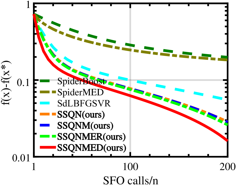
(b) Data: w8a

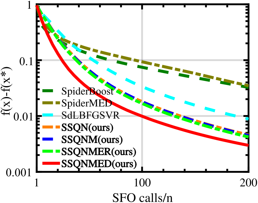
(c) Data: mnist

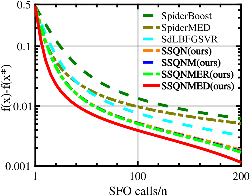
(d) Data: ijcnn1

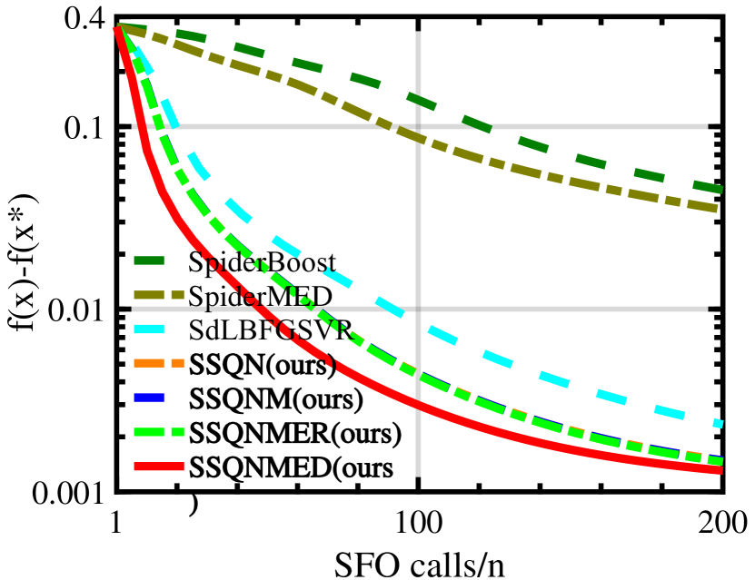
(e) Data: covtype

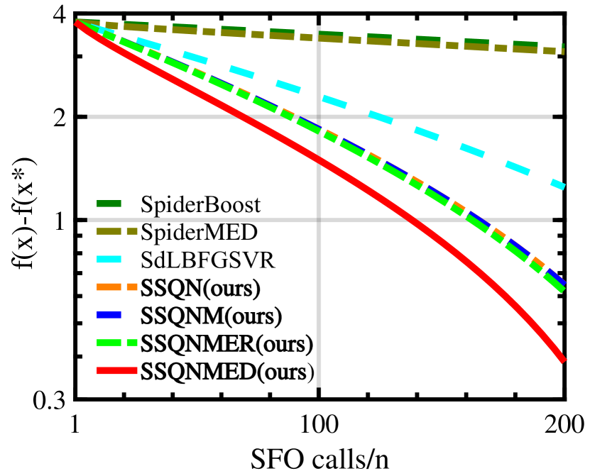
(f) Data: synthetic data

Figure 1: Comparison among algorithms for solving nonconvex SVM problems.

5.2 Convergence Analysis of Online Faster SQN Method

To study the SFO complexity of the online SpiderSQN-type of algorithms we let Assumptions 1 to 5 hold, and make an extra standard assumption (Algorithm 6).

Assumption 6

There exists a constant $\sigma_{1}>0$ such that for all $x\in\mathbb{R}^{d}$ and all random samples $u\sim\mathbb{P}$, it holds that $\mathbb{E}_{u\sim\mathbb{P}}\|\nabla f_{u}(x)-\nabla f(x)\|^{2}\leqslant\sigma_{1}^{2}$.

Assumption 6 shows that the $\nabla f_{u}(x)$ is an unbiased estimator of $\nabla f(x)$ with bounded variance. Assumption 6 is a standard assumption in online optimization analysis Zhou et al. (2019c) and is for online case only.

Theorem 7

Let additional Algorithm 6 hold. Apply Algorithm 4 to solve the online optimization problem (22). Choose any desired accuracy $\epsilon>0$ and set parameters as

$$q=|\xi_{k}|=\sqrt{|\xi_{0}|}\equiv\sqrt{\left(\frac{\eta\sigma_{\mathrm{max}}}{\beta^{*}}+2+\frac{L^{2}\eta^{3}\sigma_{\mathrm{max}}^{3}}{\beta^{*}}\right)\frac{2\sigma_{1}^{2}}{\epsilon^{2}}},$$

where $\beta^{*}=\frac{\eta\sigma_{\mathrm{min}}}{2}-\frac{L\eta^{2}\sigma_{\mathrm{max}}^{2}}{2}-\frac{\eta^{3}\sigma_{\mathrm{max}}^{3}L^{2}}{2}$, and let $\eta\equiv\frac{(1+\sqrt{5})\sigma_{\mathrm{min}}}{2L\sigma_{\mathrm{max}}^{2}}$. Then, the output $x_{\zeta}$ of this algorithm satisfies $\mathbb{E}\|\nabla f(x_{\zeta})\|\leq\epsilon$ given that the total number of iterations $K$ satisfies

$$K\geq\mathcal{O}\bigg{(}\frac{f(x_{0})-f^{*}}{\epsilon^{2}}\bigg{)}.$$ (34)

Moreover, the SFO complexity is in the order of $\mathcal{O}(\epsilon^{-3})$.

Theorem 8

Let additional Algorithm 6 hold. Apply online Algorithm 5 to solve the online optimization problem (22). Choose any desired accuracy $\epsilon>0$ and set parameters as

$$\alpha_{k}=\frac{2}{k+1},\quad q=|\xi_{k}|=\sqrt{|\xi_{0}|}\equiv\sqrt{\frac{4(1+\beta/\beta^{*})\sigma_{1}^{2}}{\epsilon^{2}}},$$

where $\beta^{*}=\beta(\frac{\sigma_{\mathrm{min}}}{2}-3L\beta\sigma_{\mathrm{max}}^{2}-3L^{2}\beta^{2}\sigma_{\mathrm{max}}^{3})$, $\beta\equiv\frac{\sigma_{\mathrm{min}}}{(3+\sqrt{15})L\sigma_{\mathrm{max}}^{2}}$. Let $\beta_{k}=\beta$, $\lambda_{k}\in[\beta_{k},(1+\alpha_{k})\beta_{k}]$. Then, the output $z_{\zeta}$ of this algorithm satisfies $\mathbb{E}\|\nabla f(z_{\zeta})\|\leq\epsilon$ provided that the total number of iterations $K$ satisfies

$$K\geq\mathcal{O}\bigg{(}\frac{f(x_{0})-f^{*}}{\epsilon^{2}}\bigg{)}.$$ (35)

Moreover, the SFO complexity is in the order of $\mathcal{O}(\epsilon^{-3})$.

Theorem 9

Let additional Algorithm 6 hold. Apply the online SpiderSQNMER or online SpiderSQNMED to solve the problem (22). Choose any desired accuracy $\epsilon>0$, let $\alpha_{k}$ defined as Eqs. (20) and (21) for online SpiderSQNMER and online SpiderSQNMED, respectively. And set parameters as

$$q=|\xi_{k}|=\sqrt{|\xi_{0}|}\equiv\sqrt{\frac{4(1+\beta/\beta^{*})\sigma_{1}^{2}}{\epsilon^{2}}},$$

where $\beta^{*}=\beta(\frac{\sigma_{\mathrm{min}}}{2}-3L\beta\sigma_{\mathrm{max}}^{2}-3L^{2}\beta^{2}\sigma_{\mathrm{max}}^{3})$, $\beta\equiv\frac{\sigma_{\mathrm{min}}}{(3+\sqrt{15})L\sigma_{\mathrm{max}}^{2}}$. Let $\beta_{k}=\beta$, $\lambda_{k}\in[\beta_{k},(1+\alpha_{k})\beta_{k}]$. Then, the output $z_{\zeta}$ of both algorithms satisfy $\mathbb{E}\|\nabla f(z_{\zeta})\|\leq\epsilon$ provided that the total number of iterations $K$ satisfies

$$K\geq\mathcal{O}\bigg{(}\frac{f(x_{0})-f^{*}}{\epsilon^{2}}\bigg{)}.$$ (36)

Moreover, the SFO complexity is in the order of $\mathcal{O}(\epsilon^{-3})$.

Remark 10

There are two differences between Algorithm 7 and Algorithm 8&9: 1) Algorithm 8&9 introduce an extra parameter, i.e., momentum coefficient $\alpha_{k}$ because of using momentum scheme; 2) the choice of $\beta_{k}$ in Algorithm 8&9 are different from that of $\eta$ in Algorithm 7 (note that $\beta_{k}$ plays a same role as $\eta$). Algorithm 8 and Algorithm 9 are the same except for the choice of $\alpha_{k}$ due to using different momentum schemes. Moreover, given required conditions in Algorithm LABEL:thm:_ssqn-online,thm:_ssqnm-online,thm:_ssqnmer-online, the SFO complexity of Algorithm 4 and its variants with different momentum schemes to satisfy the $\epsilon$-first-order stationary condition are $\mathcal{O}(\epsilon^{-3})$, which matches the state-of-the-art results of first-order stochastic methods.

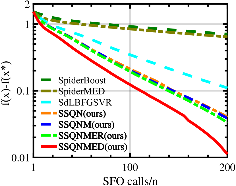
(a) Data: a9a

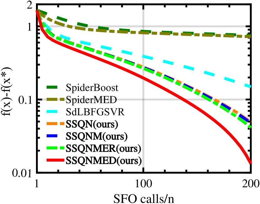
(b) Data: w8a

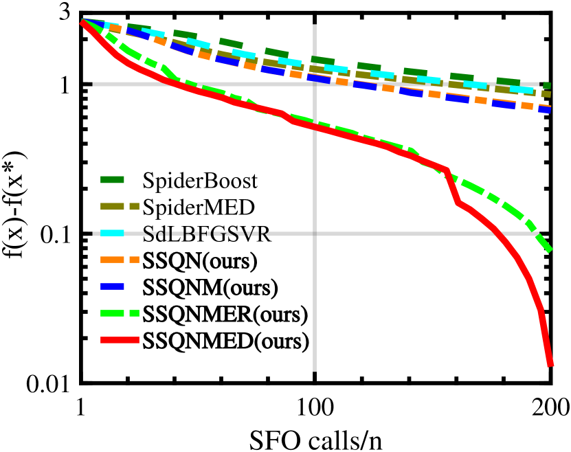
(c) Data: mnist

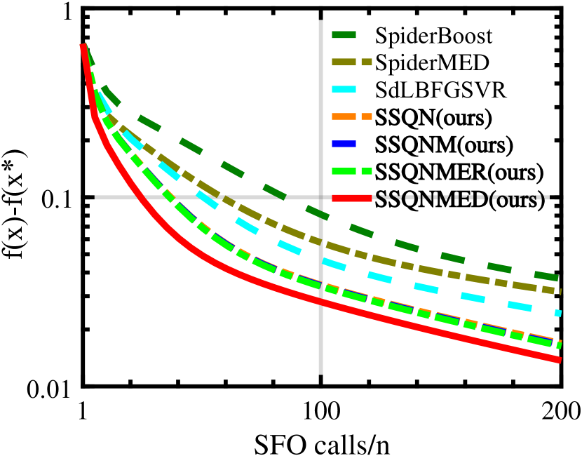
(d) Data: ijcnn1

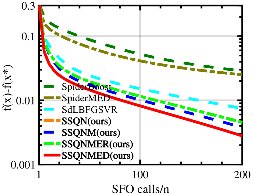
(e) Data: covtype

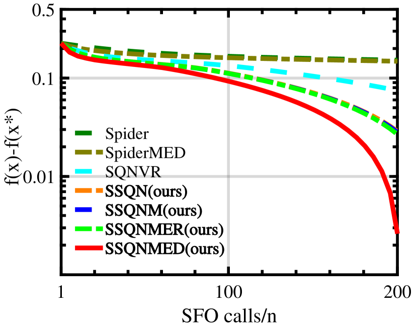
(f) Data: synthetic data

Figure 2: Comparison among algorithms for solving nonconvex robust linear regression problems.

5.3 The Lower Bound

We will present the optimality of our algorithms in the perspective of algorithmic lower bound result Carmon et al. (2017), which can be obtained by following the analyses in Fang et al. (2018). For the finite-sum case, given any random algorithm ${\mathcal{A}}$ that maps functions $f:\mathbb{R}^{d}\to\mathbb{R}$ to a sequence of iterates in $\mathbb{R}^{d+1}$, with

$$[\mathbf{x}^{k};i_{k}] ={\mathcal{A}}^{k-1}\big{(}\mathbbm{\xi},\nabla f_{i_{0}}(\mathbf{x}^{0}),\nabla f_{i_{1}}(\mathbf{x}^{1}),\ldots,\nabla f_{i_{k-1}}(\mathbf{x}^{k-1})\big{)},$$

$$\quad k\geq 1,$$ (37)

where ${\mathcal{A}}^{k}$ denotes measure mapping into $\mathbb{R}^{d+1}$, $i_{k}$ is the individual function chosen by ${\mathcal{A}}$ at iteration $k$, and $\mathbbm{\xi}$ is uniform random vector from $[0,1]$. Moreover, there is $[\mathbf{x}^{0};i_{0}]={\mathcal{A}}^{0}(\mathbbm{\xi})$, where ${\mathcal{A}}^{0}$ is a measure mapping. The lower bound result for solving (LABEL:eq:_P) is stated in Theorem 11.

Theorem 11 (Lower bound for SFO complexity for the finite-sum case)

Fang et al. (2018) For any $L>0$, $\Delta>0$, and $2\leq n\leq\mathcal{O}\left(\Delta^{2}L^{2}\cdot\epsilon^{-4}\right)$, for any algorithm ${\mathcal{A}}$ satisfying (5.3), there exists a dimension $d={\mathcal{O}}\big{(}\Delta^{2}L^{2}\cdot n^{2}\epsilon^{-4}\big{)},$ and a function $f$ satisfying Assumptions 1-6 for the finite-sum case, such that in order to find an $\epsilon$-first-order stationary point must cost at least $\mathcal{O}\big{(}L\Delta\cdot n^{1/2}\epsilon^{-2}\big{)}$ stochastic gradient accesses.

Note that the condition $n\leq\mathcal{O}(\epsilon^{-4})$ in Theorem 11 ensures the lower bound $\mathcal{O}(n^{1/2}\epsilon^{-2})=\mathcal{O}(n+n^{1/2}\epsilon^{-2})$. Therefore, the upper bound in Theorem 3 matches the lower bound in Theorem 11 up to a constant factor of relevant parameters, and is thus near-optimal. The proof of Theorem 11 provided in the Appendix utilizes a specific counterexample function that requires at least $\mathcal{O}(n^{1/2}\epsilon^{-2})$ stochastic gradient accesses, which is inspired by Fang et al. (2018); Carmon et al. (2017); Nesterov (2018).

Remark 12

Through setting $n=\mathcal{O}(\epsilon^{-4})$ the lower bound complexity in Theorem 11 can achieve $\mathcal{O}(\epsilon^{-4})$. It is necessary to emphasize that this does not violate the upper bound in the online case, i.e. $\mathcal{O}(\epsilon^{-3})$ (Theorems 7-9), since the counterexample established in the lower bound depends not on the stochastic gradient variance $\sigma_{1}^{2}$ specified in Assumption 6 but the example number $n$. To obtain the lower bound result for the online case with the additional Assumption 6, one can just construct a counterexample that requires $\mathcal{O}({\epsilon}^{-3})$ stochastic gradient accesses with the knowledge of $\sigma_{1}^{2}$ instead of $n$.

5.4 Computational Complexity

In the following, we will analyze the time complexity of the proposed algorithms and show that the extra computation costs of computing inverse Hessian approximation matrix and using momentum acceleration are negligible.

First, we analyze the computational cost of Algorithm 1. In Step 1, the computation of $\gamma_{k}^{-1}$ involves two inner product, which takes $2d$ multiplications. In Step 2, the computation involves two inner product and one scalar-vector product, which takes $3d$ multiplications. First recursive loop (i.e., Steps 3 to 5) involves $2m$ scalar-vector multiplications and $m$ vector inner products, which takes $3md$ multiplications. So does the second loop (i.e., Steps 8 to 10). Step 7 involving a scalar-vector product takes $d$ multiplications. Therefor, the whole procedure takes $(6m+6)d$ multiplications.

Then, we turn to Algorithm 3. Step 4 involves scalar-vector products, which takes $2d$ multiplications. In Step 6, the computation of full gradient takes at least $2nd$ multiplications. In Step 8, the computation of stochastic gradients with batch-size $n^{1/2}$ takes $2n^{1/2}d$ multiplications. In Steps 10, $(6m+6)d$ multiplications are necessary for calling Algorithm 1. Steps 11 and 12 involving scalar-vector products need $d$ multiplications. Therefore, the total computational cost in an outer loop involves $[(6m+6)q+2n+2n^{1/2}q+4q]d$ multiplications.

Based on above analyses, the computational cost of other algorithms can be obtained easily. For algorithms without momentum acceleration, one needs to omit the extra computation cost ($2d$ multiplications) of computing momentum term. As for algorithms without using approximate Hessian information, one needs to omit the extra computational cost of calling Algorithm 1.

We summarize the computational complexity of each algorithm during an outer loop with $q$ iterations (for finite-sum case there is $\mathcal{O}(q)=\mathcal{O}(n^{1/2})$, while for online case there is $\mathcal{O}(q)=\mathcal{O}(\epsilon^{-1})$) in Table 2. As shown in Table 2, for finite-sum case, the extra computation costs of computing approximate Hessian information and using momentum acceleration take up $\frac{mn^{1/2}}{n+mn^{1/2}}$ in the whole procedure. Since $m$ usually ranges from 5 to 20 as suggested in Nocedal and Wright (2006) and $n$ is sufficiently large in big data situation, the extra computation thus is negligible. So does the online case, when $\epsilon$ is considerably small. Note that for analyses convenience, we reasonably assume $2d$ multiplications are needed when computing a stochastic gradient for general machine learning problem.

6 Experiments

In this section, to demonstrate the promising performance of the proposed algorithms, we compare our methods with some state-of-the-art stochastic quasi-Newton algorithms and stochastic first-order algorithms for nonconvex optimization. Following are brief introductions of algorithms used in our experiments. SpiderBoost Wang et al. (2018b): SpiderBoost is a boosting version of SPIDER, which takes up a more aggressive stepsize than SPIDER and thus outperforms SPIDER in practice. SdLBFGSVR Wang et al. (2017): SdLBFGSVR is a SQN method (more specifically, stochastic damped L-BFGS method) equipped with the SVRG variance reduction technique. SpiderMED Zhou et al. (2019c): ProxSPIDER-MED Zhou et al. (2019c) is a proximal method that uses the epochwise-diminishing momentum scheme to improve the practical performance of SpiderBoost. Especially, ProxSPIDER-MED is the faster one among all momentum variants of SpiderBoost proposed in Zhou et al. (2019c). Since our paper does not touch upon nonconvex nonsmooth optimization, we adopt the ProxSPIDER-MED without proximal operator and call it SpiderMED. Our methods: Our methods include four SpiderSQN (SSQN) type of methods, i.e., SSQN (Aslgorithm 2), SSQN with vanilla momentum scheme (SSQNM, i.e.., Algorithm 3), SSQN with epochwise-restart momentum (SSQNMER) and SSQN with epochwise-diminishing momentum (SSQNMED). Note that SSQNMER and SSQNMED are proposed in section 3.3.

Follow the experiment setting in Zhou et al. (2019c), we choose a fixed mini-batch size $256$ and the epoch length $q$ is set to $2n/256$. When implement the SdLBFGS Wang et al. (2017), we set the memory size to $m=5$ as suggested in Nocedal and Wright (2006), and fix the $\sigma$ for each comparison. Moreover, we implement experiments on synthetic data for the complement of real datasets, which are generated as Wang et al. (2017). Generating Synthetic Data: The training and testing points $(a,b)$ are generated in the following manner. First, we generate a sparse vector $a$ with 5% nonzero components following the uniform distribution on $[0,1]^{n}$, and then set $b=\text{sign}({u},a)$ for some $u\in\mathbb{R}^{n}$ drawn from the uniform distribution on $[-1,1]^{n}$. Descriptions of Datasets: We implement all experiments on five public datasets from the LIBSVM Chang and Lin (2011) and a synthetic data as the complement to these public datasets is summarized in Algorithm 3. Especially, as for the mnist dataset we use the one-vs-rest technique to convert it to a binary class data.

Table 3: Descriptions of Datasets.

datasets	#samples	#features	#classes
a9a	32,561	123	2
w8a	64,700	300	2
ijcnn1	141,691	22	2
mnist	60,000	780	2
covtype	581,012	54	2
synthetic data	100,000	5,000	2

6.1 Nonconvex Support Vector Machine

First, above algorithms are applied to solve the nonconvex support vector machine (SVM) problem with a sigmoid loss function:

$$\min_{x\in\mathbb{R}^{d}}f(x):=\frac{1}{n}\sum_{i=1}^{n}(1-\mathrm{tanh}(b_{i}\left\langle x,a_{i}\right\rangle))+r\|x\|^{2},$$

where $a_{i}\in\mathbb{R}^{d}$ denotes the $i$-th sample and $b_{i}\in{\pm 1}$ is the corresponding label. In the experiments, the learning rate $\eta$ and regular coefficient $r$ for all algorithms are both fixed as $0.001$. Moreover, in algorithms with momentum scheme $\beta_{k}$ is fixed as $\eta$, and $\lambda_{k}$ remains the same for each comparison.

The experiment results on those four datasets are shown in Fig. 1, where $f(x)$ is the function value and $f(x^{*})$ is a suitable constant for each case. First, as for datasets w8a and ijcnn1 the initial solutions to all algorithms are drawn from the standard norm distribution, while for datasets a9a and mnist they take the original point. As Fig. 1 depicts, all these stochastic quasi-Newton methods (including SdlBFGSVR and four SpiderSQN (SSQN)-type of algorithms) outperform stochastic first-order methods (including Spider and SpiderMED) by a considerably large margin, which demonstrates the promising nature of stochastic quasi-Newton methods for nonconvex optimization. And one can see that the basic algorithm SSQN converges more faster than SdLBFGSVR, which is corresponding to the theoretical result that the proposed method has a lower SFO complexity than SdLBFGSVR. Meanwhile, among the four SSQN-type of algorithms, three algorithms with different momentum schemes all have a better performance than the SSQN. Moreover, among these three algorithms, the one using epochwise-diminishing momentum (SSQNMED) achieves the best performance, while the one using the iterationwise-diminishing momentum (SSQNM) achieves the poorest.

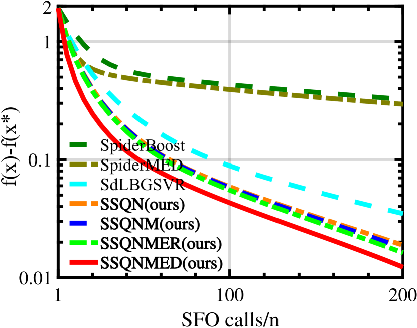
(a) Data: a9a

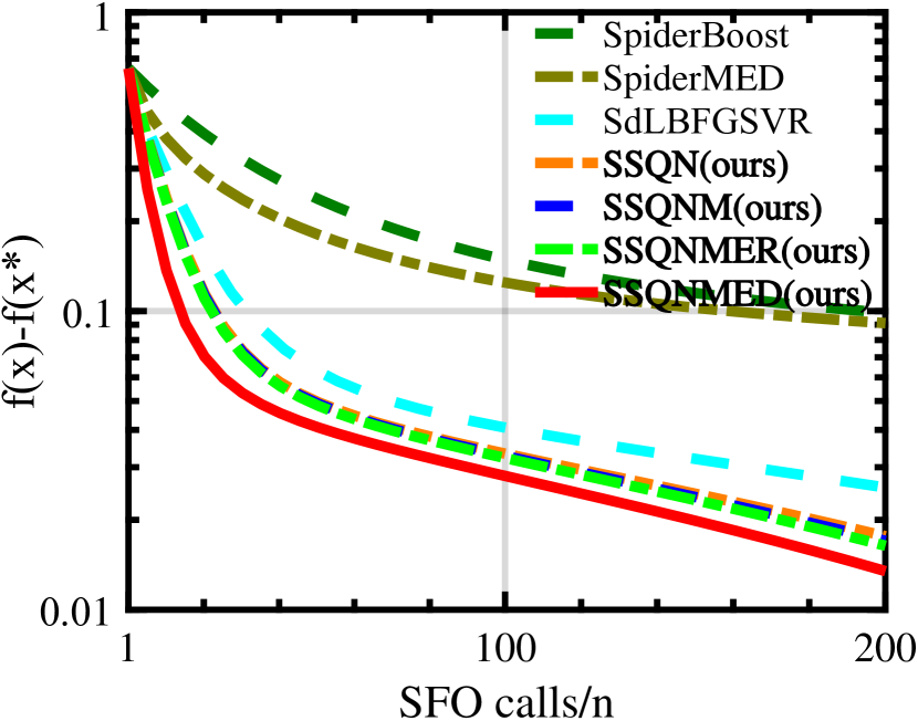
(b) Data: w8a

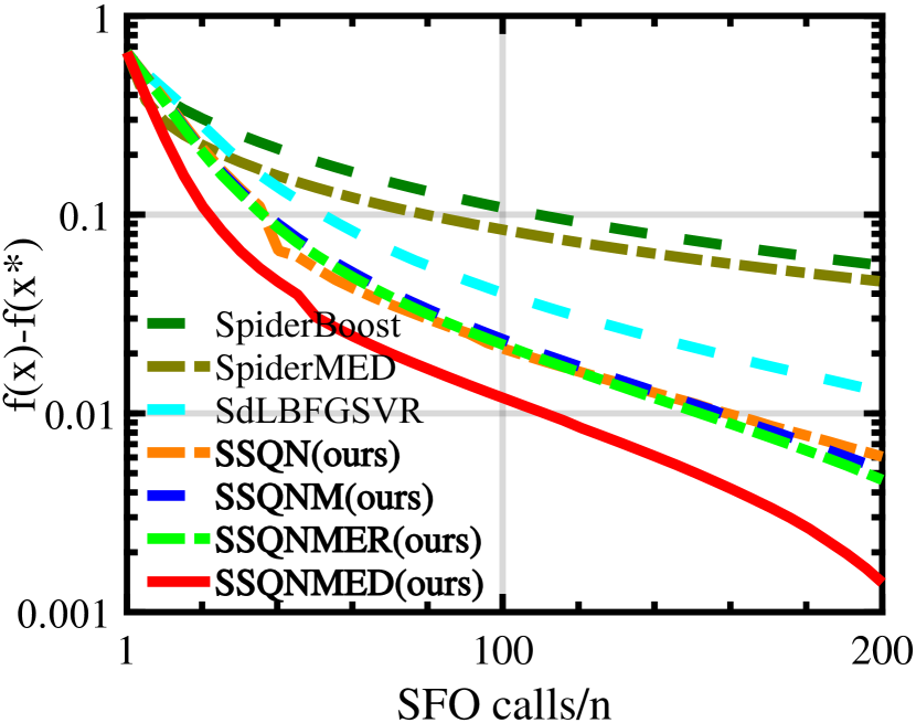
(c) Data: mnist

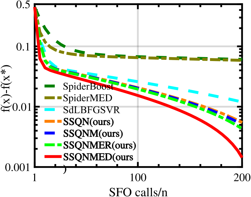
(d) Data: ijcnn1

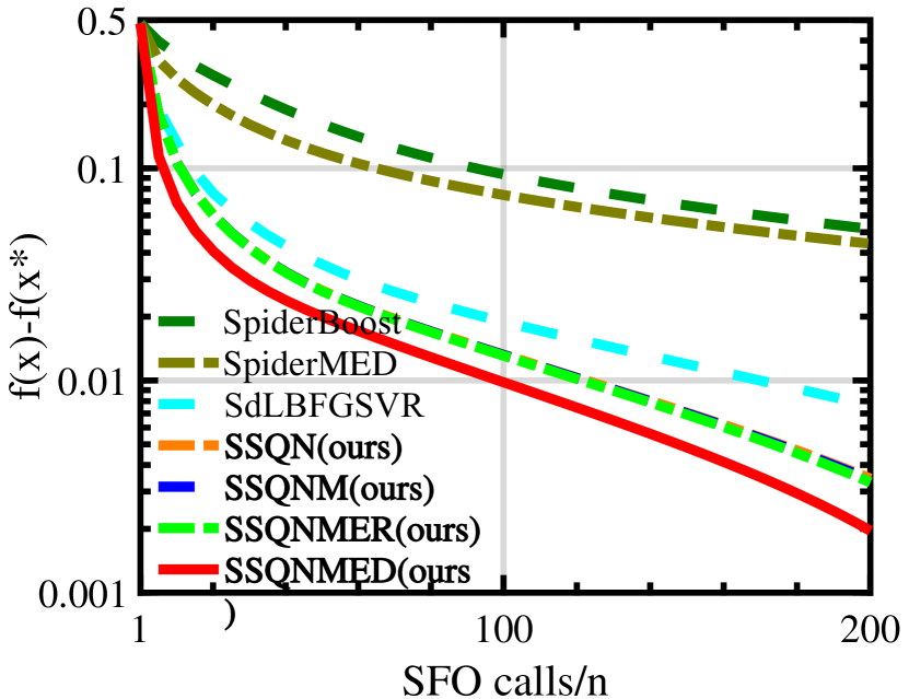
(e) Data: covtype

(f) Data: synthetic data

Figure 3: Comparison among algorithms for solving nonconvex logistic regression problems.

6.2 Nonconvex Robust Linear Regression

We consider comparing these algorithms for solving such a nonconvex robust linear regression problem:

$$\min_{x\in\mathbb{R}^{d}}f(x):=\frac{1}{n}\sum_{i=1}^{n}\ell(b_{i}-\left\langle x,a_{i}\right\rangle),$$

where the nonconvex loss function is defined as $\ell(x):=\log(\frac{x^{2}}{2}+1)$. The experiment settings are same as those in the nonconvex SVM problem, except that the initial solutions in all cases are drawn from the standard norm distribution. The learning curves on the gap between $f(x)$ and $f(x^{*})$ are reported in Fig. 2. As one can see from Fig. 2, the stochastic quasi-Newton methods still have a significantly better performance than the stochastic first-order methods. Also, the proposed four SSQN-type algorithms outperform the SdLBFGSVR with a considerably large margin. In most cases, SSQNMED outperforms SSQNM and SSQNMER by a large gap, except in the dataset mnist where SSQNMER and SSQNMED have similar performances and are both significantly better than that of SSQNM.

6.3 Nonconvex Logistic Regression

Comparisons are conducted among all algorithms for solving a nonconvex logistic regression problem:

$$\min_{x\in\mathbb{R}^{d}}f(x):=\frac{1}{n}\sum_{i=1}^{n}\ell(b_{i},\left\langle x,a_{i}\right\rangle)+r\sum_{i=1}^{d}\frac{x_{i}^{2}}{1+x_{i}^{2}},$$

where the loss function $\ell$ is set to be the cross-entropy loss. For this problem, the initial solutions to all algorithms on datasets w8a and a9a are drawn from the standard norm distribution, while experiments on datasets ijcnn1 and mnist take the original point. Other experiment settings are same as those of the nonconvex SVM problem. The learning curves on the gap between $f(x)$ and $f(x^{*})$ are reported in Fig. 3. Obviously, the stochastic quasi-Newton methods outperform those stochastic first-order methods by a significantly large gap. Meanwhile, the proposed four SSQN-type of algorithms all have a better performance than the SdLBFGSVR. As for the four SSQN-type of algorithms, their performance is related to the momentum coefficient setting which means that algorithm with a larger momentum coefficient will converge faster. Moreover, in all cases the SSQNMED has the best performance among four SSQN-type algorithms, and SSQN has the worst.

7 Conclusion

In the paper, we presented the novel faster stochastic quasi-Newton (SpiderSQN) methods. Moreover, we proved that the SpiderSQN methods reach the best known SFO complexity of $\mathcal{O}(\min(n+n^{1/2}\epsilon^{-2},\epsilon^{-3}))$ for finding an $\epsilon$-approximated stationary point. At the same time, we studied the lower bound of SFO complexity of the SpiderSQN methods. As presented in the theoretical results, our methods reach the near-optimal SFO complexity in solving the nonconvex problems. Moreover, we applied three different momentum schemes to SpiderSQN to further improve its practical performance.

A Proof of Algorithm 3

Throughout the paper, let $n_{k}=\lceil k/q\rceil$ such that $(n_{k}-1)q\leq k\leq n_{k}q-1$. Note that this convergence analysis is mainly following Fang et al. (2018). We first present an auxiliary lemma from Fang et al. (2018).

Lemma 13 (Fang et al. (2018), Lemma 1)

Under Assumptions 1 and 2, the SPIDER estimator satisfies for all $(n_{k}-1)q+1\leq k\leq n_{k}q-1$,

$$\mathbb{E}\|v_{k}-\nabla f(x_{k})\|^{2}\leq\frac{L^{2}}{|\xi_{k}|}\mathbb{E}\|x_{k}-x_{k-1}\|^{2}+\mathbb{E}\|v_{k-1}-\nabla f(x_{k-1})\|^{2}.$$ (45)

Telescoping Algorithm 13 over $k$ from $(n_{k}-1)q+1$ to $k$, we obtain that

$$\mathbb{E}\|v_{k}-\nabla f(x_{k})\|^{2} \leq\sum_{i=(n_{k}-1)q}^{k-1}\frac{L^{2}}{|\xi_{k}|}\mathbb{E}\|x_{i+1}-x_{i}\|^{2}+\mathbb{E}\|v_{(n_{k}-1)q}-\nabla f(x_{(n_{k}-1)q})\|^{2}$$

$$\leq\sum_{i=(n_{k}-1)q}^{k}\frac{L^{2}}{|\xi_{k}|}\mathbb{E}\|x_{i+1}-x_{i}\|^{2}+\mathbb{E}\|v_{(n_{k}-1)q}-\nabla f(x_{(n_{k}-1)q})\|^{2}.$$ (46)

Note that the above inequality also holds for $k=(n_{k}-1)q$, which can be simply checked by plugging $k=(n_{k}-1)q$ into above inequality. As for finite-sum case, when $\textrm{mod}(k,q)=0$ there is $v_{k}=\nabla f(x_{k})$ for all $k$ such that $\mathbb{E}\|v_{k}-\nabla f(x_{k})\|^{2}=0$, and then we obtain the following bound for finite-sum case

Lemma 14

Under Assumptions 1 and 2, the SPIDER estimator satisfies for all $k\in\mathbb{N}$,

$$\mathbb{E}\|v_{k}-\nabla f(x_{k})\|^{2}\leq\sum_{i=(n_{k}-1)q}^{k-1}\frac{L^{2}}{|\xi_{k}|}\mathbb{E}\|x_{i+1}-x_{i}\|^{2}\leq\sum_{i=(n_{k}-1)q}^{k}\frac{L^{2}}{|\xi_{k}|}\mathbb{E}\|x_{i+1}-x_{i}\|^{2}$$ (47)

Then, we return to the proof of Algorithm 3.

Proof  Consider any iteration $k$ of the algorithm. By smoothness of $f$, we obtain that

$$f(x_{k}) \overset{(i)}{\leq}f(x_{k-1})+\left\langle\nabla f(x_{k-1}),x_{k}-x_{k-1}\right\rangle+\frac{L}{2}\|x_{k}-x_{k-1}\|^{2}$$

$$=f(x_{k-1})+\left\langle\nabla f(x_{k-1}),-\eta H_{k-1}v_{k-1}\right\rangle+\frac{L\eta^{2}}{2}\|H_{k-1}v_{k-1}\|^{2}$$

$$=f(x_{k-1})-\eta\left\langle\nabla f(x_{k-1})-v_{k-1},H_{k-1}v_{k-1}\right\rangle-\eta\left\langle v_{k-1},H_{k-1}v_{k-1}\right\rangle+\frac{L\eta^{2}}{2}\|H_{k-1}v_{k-1}\|^{2}$$

$$\overset{(ii)}{\leq}f(x_{k-1})-\eta\left\langle\nabla f(x_{k-1})-v_{k-1},H_{k-1}v_{k-1}\right\rangle-\eta\|v_{k-1}\|\|H_{k-1}v_{k-1}\|+\frac{L\eta^{2}}{2}\|H_{k-1}v_{k-1}\|^{2},$$ (48)

where (i) uses the Lipschitz continuity of $\nabla f$ and (ii) follows from $\left\langle a,b\right\rangle\leq\|a\|\|b\|$. Rearranging the above inequality yields that

$$f(x_{k}) \leq f(x_{k-1})-\eta(\|H_{k-1}\|-\frac{L\eta\|H_{k-1}\|^{2}}{2})\|v_{k-1}\|^{2}+\eta\|H_{k-1}\|\|\nabla f(x_{k-1})-v_{k-1}\|\|v_{k-1}\|$$

$$\overset{(i)}{\leq}f(x_{k-1})-\eta(\|H_{k-1}\|-\frac{L\eta\|H_{k-1}\|^{2}}{2})\|v_{k-1}\|^{2}+\frac{\eta\|H_{k-1}\|}{2}(\|\nabla f(x_{k-1})-v_{k-1}\|^{2}+\|v_{k-1}\|^{2})$$

$$\overset{(ii)}{\leq}f(x_{k-1})-\eta(\frac{\sigma_{\mathrm{min}}}{2}-\frac{L\eta\sigma_{\mathrm{max}}^{2}}{2})\|v_{k-1}\|^{2}+\frac{\eta\sigma_{\mathrm{max}}}{2}\|\nabla f(x_{k-1})-v_{k-1}\|^{2}.$$ (49)

where (i) uses the inequality that $\left\langle x,y\right\rangle\leq\frac{\|x\|^{2}+\|y\|^{2}}{2}$ for $x,y\in\mathbb{R}^{d}$, (ii) follows from Assumption 4. Taking expectation on both sides of the above inequality yields that

$$\mathbb{E} f(x_{k+1})$$

$$\leq\mathbb{E}f(x_{k})+\frac{\eta\sigma_{\mathrm{max}}}{2}\mathbb{E}\|\nabla f(x_{k})-v_{k}\|^{2}-(\frac{\eta\sigma_{\mathrm{min}}}{2}-\frac{L\eta^{2}\sigma_{\mathrm{max}}^{2}}{2})\mathbb{E}\|v_{k}\|^{2}$$

$$\overset{(i)}{\leq}\mathbb{E}f(x_{k})+\frac{\eta\sigma_{\mathrm{max}}}{2}\sum_{i=(n_{k}-1)q}^{k}\frac{L^{2}}{|\xi_{k}|}\mathbb{E}\|x_{i+1}-x_{i}\|^{2}-(\frac{\eta\sigma_{\mathrm{min}}}{2}-\frac{L\eta^{2}\sigma_{\mathrm{max}}^{2}}{2})\mathbb{E}\|v_{k}\|^{2}$$

$$\overset{(ii)}{=}\mathbb{E}f(x_{k})+\frac{\eta^{3}\sigma_{\mathrm{max}}^{3}}{2}\sum_{i=(n_{k}-1)q}^{k}\frac{L^{2}}{|\xi_{k}|}\mathbb{E}\|v_{i}\|^{2}-(\frac{\eta\sigma_{\mathrm{min}}}{2}-\frac{L\eta^{2}\sigma_{\mathrm{max}}^{2}}{2})\mathbb{E}\|v_{k}\|^{2},$$ (50)

where (i) follows from Eq. (47), and (ii) follows from the facts that $x_{k+1}=x_{k}-\eta H_{k}v_{k}$ and Algorithm 4. Next, telescoping Eq. (50) over $k$ from $(n_{k}-1)q$ to $k$ where $k\leq n_{k}q-1$ and noting that for $(n_{k}-1)q\leq j\leq n_{k}q-1$, $n_{j}=n_{k}$ , we obtain

$$\mathbb{E} f(x_{k+1})$$

$$\leq\mathbb{E}f(x_{(n_{k}-1)q})+\frac{\eta^{3}\sigma_{\mathrm{max}}^{3}}{2}\sum_{j=(n_{k}-1)q}^{k}\sum_{i=(n_{k}-1)q}^{j}\frac{L^{2}}{|\xi_{k}|}\mathbb{E}\|v_{i}\|^{2}-(\frac{\eta\sigma_{\mathrm{min}}}{2}-\frac{L\eta^{2}\sigma_{\mathrm{max}}^{2}}{2})\sum_{j=(n_{k}-1)q}^{k}\mathbb{E}\|v_{j}\|^{2}$$

$$\overset{(i)}{\leq}\mathbb{E}f(x_{(n_{k}-1)q})+\frac{\eta^{3}\sigma_{\mathrm{max}}^{3}}{2}\sum_{j=(n_{k}-1)q}^{k}\sum_{i=(n_{k}-1)q}^{k}\frac{L^{2}}{|\xi_{k}|}\mathbb{E}\|v_{i}\|^{2}-(\frac{\eta\sigma_{\mathrm{min}}}{2}-\frac{L\eta^{2}\sigma_{\mathrm{max}}^{2}}{2})\sum_{j=(n_{k}-1)q}^{k}\mathbb{E}\|v_{j}\|^{2}$$

$$\overset{(ii)}{\leq}\mathbb{E}f(x_{(n_{k}-1)q})+\frac{\eta^{3}\sigma_{\mathrm{max}}^{3}L^{2}q}{2|\xi_{k}|}\sum_{i=(n_{k}-1)q}^{k}\mathbb{E}\|v_{i}\|^{2}-(\frac{\eta\sigma_{\mathrm{min}}}{2}-\frac{L\eta^{2}\sigma_{\mathrm{max}}^{2}}{2})\sum_{j=(n_{k}-1)q}^{k}\mathbb{E}\|v_{j}\|^{2}$$

$$=\mathbb{E}f(x_{(n_{k}-1)q})-\sum_{i=(n_{k}-1)q}^{k}\left(\frac{\eta\sigma_{\mathrm{min}}}{2}-\frac{L\eta^{2}\sigma_{\mathrm{max}}^{2}}{2}-\frac{\eta^{3}\sigma_{\mathrm{max}}^{3}L^{2}q}{2|\xi_{k}|}\right)\mathbb{E}\|v_{i}\|^{2}$$

$$\overset{(iii)}{=}\mathbb{E}f(x_{(n_{k}-1)q})-\sum_{i=(n_{k}-1)q}^{k}\beta^{*}\mathbb{E}\|v_{i}\|^{2},$$ (51)

where (i) extends the summation of the second term from $j$ to $k$, (ii) follows from the fact that $k\leqslant n_{k}q-1$. Thus, we obtain

$$\sum_{j=(n_{k}-1)q}^{k} \sum_{i=(n_{k}-1)q}^{k}\frac{L^{2}}{|\xi_{k}|}\mathbb{E}\|v_{i}\|^{2}\leq\frac{(k+q-n_{k}q+1)L^{2}}{|\xi_{k}|}\sum_{i=(n_{k}-1)q}^{k}\mathbb{E}\|v_{i}\|^{2}\leq\frac{qL^{2}}{|\xi_{k}|}\sum_{i=(n_{k}-1)q}^{k}\mathbb{E}\|v_{i}\|^{2},$$ (52)

and (iii) follows from $\beta^{*}=\frac{\eta\sigma_{\mathrm{min}}}{2}-\frac{L\eta^{2}\sigma_{\mathrm{max}}^{2}}{2}-\frac{\eta^{3}\sigma_{\mathrm{max}}^{3}L^{2}q}{2|\xi_{k}|}$.

We continue the proof by further driving

$$\mathbb{E}f(x_{K})- \mathbb{E}f(x_{0})$$

$$=(\mathbb{E}f(x_{q})-\mathbb{E}f(x_{0}))+(\mathbb{E}f(x_{2q})-\mathbb{E}f(x_{q}))+\cdots+(\mathbb{E}f(x_{K})-\mathbb{E}f(x_{(n_{k}-1)q}))$$

$$\overset{(i)}{\leq}\sum_{i=0}^{q-1}\beta^{*}\mathbb{E}\|v_{i}\|^{2}-\sum_{i=q}^{2q-1}\beta^{*}\mathbb{E}\|v_{i}\|^{2}-\cdots-\sum_{i=(n_{K}-1)q}^{K-1}\beta^{*}\mathbb{E}\|v_{i}\|^{2}$$

$$=\sum_{i=0}^{K-1}\beta^{*}\mathbb{E}\|v_{i}\|^{2},$$ (53)

where (i) follows from Eq. (51). Note that $\mathbb{E}f(x_{K})\geq f^{*}\triangleq\inf_{x\in\mathbb{R}^{d}}f(x)$. Hence, the above inequality implies that

$$\sum_{i=0}^{K-1}\beta^{*}\mathbb{E}\|v_{i}\|^{2}\leq f(x_{0})-f^{*}.$$ (54)

We next bound $\mathbb{E}\|\nabla f(x_{\xi})\|^{2}$, where $\xi$ is selected uniformly at random from $\{0,\ldots,K-1\}$. Observe that

$$\mathbb{E}\|\nabla f(x_{\xi})\|^{2}=\mathbb{E}\|\nabla f(x_{\xi})-v_{\xi}+v_{\xi}\|^{2}\leq 2\mathbb{E}\|\nabla f(x_{\xi})-v_{\xi}\|^{2}+2\mathbb{E}\|v_{\xi}\|^{2}.$$ (55)

Next, we bound the two terms on the right hand side of the above inequality. First, note that

$$\mathbb{E}\|v_{\xi}\|^{2}=\frac{1}{K}\sum_{i=0}^{K-1}\mathbb{E}\|v_{i}\|^{2}\leq\frac{f(x_{0})-f^{*}}{K\beta^{*}},$$ (56)

where the last inequality follows from Eq. (54). On the other hand, note that

$$\mathbb{E}\|\nabla f(x_{\xi})-v_{\xi}\|^{2} \overset{(i)}{\leq}\mathbb{E}\sum_{i=(n_{\xi}-1)q}^{\xi}\frac{L^{2}}{|\xi_{k}|}\mathbb{E}\|x_{i+1}-x_{i}\|^{2}+\mathbb{E}\sum_{i=(n_{\xi}-1)q}^{\xi}\frac{L^{2}\eta^{2}\sigma_{\mathrm{max}}^{2}}{|\xi_{k}|}\mathbb{E}\|v_{i}\|^{2}$$

$$\overset{(iii)}{\leq}\mathbb{E}\sum_{i=(n_{\xi}-1)q}^{\min\{(n_{\xi})q-1,K-1\}}\frac{L^{2}\eta^{2}\sigma_{\mathrm{max}}^{2}}{|\xi_{k}|}\mathbb{E}\|v_{i}\|^{2}\overset{(iv)}{\leq}\frac{q}{K}\sum_{i=0}^{K-1}\frac{L^{2}\eta^{2}\sigma_{\mathrm{max}}^{2}}{|\xi_{k}|}\mathbb{E}\|v_{i}\|^{2}$$

$$\overset{(v)}{\leq}\frac{L^{2}\eta^{2}\sigma_{\mathrm{max}}^{2}q}{K|\xi_{k}|\beta^{*}}\left(f(x_{0})-f^{*}\right),$$ (57)

where (i) follows from Eqs. (46) and (47), (ii) follows from the fact that $x_{k+1}=x_{k}-\eta H_{k}v_{k}$ and Assumption 4, (iii) follows from the definition of $n_{\xi}$, which implies $\xi\leqslant\min\{(n_{\xi})q-1,K-1\}$, (iv) follows from the fact that the probability that $n_{\xi}=1,2,\cdots,n_{K}$ is less than or equal to $q/(K)$, and (v) follows from Eq. (56).

Substituting Eqs. (56) and (57) into Eq. (55), we obtain

$$\mathbb{E}\|\nabla f(x_{\xi})\|^{2} \leq\frac{2\left(f(x_{0})-f^{*}\right)}{K\beta^{*}}+\frac{2L^{2}\eta^{2}\sigma_{\mathrm{max}}^{2}q}{K|\xi_{k}|\beta^{*}}\left(f(x_{0})-f^{*}\right)$$

$$=\frac{2}{K\beta^{*}}\left(1+\frac{L^{2}\eta^{2}\sigma_{\mathrm{max}}^{2}q}{|\xi_{k}|}\right)\left(f(x_{0})-f^{*}\right).$$ (58)

 

Next we set the parameters as

$$S_{1}=n,q=\sqrt{n},\xi_{k}=\sqrt{n},\text{ and }\eta=\frac{c}{L\sigma_{\mathrm{max}}m}\ ,$$ (59)

where $c=\sigma_{\mathrm{min}}/\sigma_{\mathrm{max}}\leq 1$, and $m=(1+\sqrt{5})/2$. Given the parameters setting of $S_{1}$, $q$, and $\xi_{k}$ the value of $m$ is determined as follow

$$\beta^{*} =\frac{\eta\sigma_{\mathrm{min}}}{2}-\frac{L\eta^{2}\sigma_{\mathrm{max}}^{2}}{2}-\frac{\eta^{3}\sigma_{\mathrm{max}}^{3}L^{2}}{2}$$

$$\overset{}{=}\frac{1}{2L}({L\eta\sigma_{\mathrm{min}}}-{L^{2}\eta^{2}\sigma_{\mathrm{max}}^{2}}-{\eta^{3}\sigma_{\mathrm{max}}^{3}L^{3}})$$

$$\overset{(i)}{=}\frac{c^{2}}{2Lm^{3}}(m^{2}-m-c)$$

where (i) follows from the definition of $\eta$ together with the problem independent parameter $c=\sigma_{\mathrm{min}}/\sigma_{\mathrm{max}}\leq 1$. When $c=1$ this reduces to the SpiderBoost algorithm with steosize $\eta$ scaled by $\sigma_{\mathrm{min}}$ (or $\sigma_{\mathrm{max}}$). Next, we should determine a suitable value of $m$ to ensure $\beta^{*}>0$ i.e.,

$$\beta^{*} \overset{}{=}\frac{c^{2}}{2Lm^{3}}(m^{2}-m-c)>0$$

it is sufficient to ensure $m^{2}-m-c>0$. Thus, we obtain $m>(1+\sqrt{1+4c})/2$. In the Spider-SQN method there is $c<1$, and we can let $m=(1+\sqrt{5})/2$. Plugging $m=(1+\sqrt{5})/2$ into Eq. (LABEL:beta1) we obtain

$$\beta^{*}=\frac{c^{2}}{2Lm^{3}}(1-c)>0.$$ (62)

therefore, $m=(1+\sqrt{5})/2$ is reasonable and thus $\eta=\frac{(1+\sqrt{5})\sigma_{\mathrm{min}}}{2L\sigma_{\mathrm{max}}^{2}}$. Plugging Eqs. (59) and (62) into Eq. (58), we obtain that, after $K$ iterations, the output of SpiderBoost satisfies

$$\mathbb{E}\|\nabla f(x_{\zeta})\|^{2}\leq\frac{2(1+\frac{c^{2}}{m^{2}})}{K\beta^{*}}\left(f(x_{0})-f^{*}\right)$$ (63)

To ensure $\mathbb{E}\|\nabla f(x_{\zeta})\|\leqslant\epsilon$, it is sufficient to ensure $\mathbb{E}\|\nabla f(x_{\zeta})\|^{2}\leqslant\epsilon^{2}$ (because $\left(\mathbb{E}\|\nabla f(x_{\zeta})\|\right)^{2}\leq\mathbb{E}\|\nabla f(x_{\xi})\|^{2}$ due to Jensen’s inequality). Thus, we need the total number $K$ of iterations satisfies that $\frac{2(1+\frac{c^{2}}{m^{2}})}{K\beta^{*}}\left(f(x_{0})-f^{*}\right)\leq\epsilon^{2}$, which gives

$$K=\frac{2(1+\frac{c^{2}}{m^{2}})/\beta^{*}}{\epsilon^{2}}\left(f(x_{0})-f^{*}\right).$$ (64)

Then, the total SFO complexity is given by

$$\left\lceil\frac{K}{q}\right\rceil\cdot S_{1}+K\cdot\xi_{k}\leqslant(K+q)\cdot\frac{S_{1}}{q}+K\cdot\xi_{k}=K\sqrt{n}+n+K\sqrt{n}=O(\sqrt{n}\epsilon^{-2}+n),$$

where the last equation follows from Eq. (64), thus the SFO complexity of Algorithm 2 is $O(\sqrt{n}\epsilon^{-2}+n)$.

B Proof of Algorithm 4

B.1 Auxiliary Lemmas for Analysis of Algorithm 3

Note that in algorithm utilizing momentum scheme the $\beta_{k}$ remains the same for all $k$, thus we use $\beta$ for notation brevity. First, we collect some auxiliary results that facilitate the analysis of Algorithm 3. For any $k\in\mathbb{N}$, denote $\tau(k)\in\mathbb{N}$ the unique integer such that $(\tau(k)-1)q\leq k\leq\tau(k)q-1$. We also define $\Gamma_{0}=0,\Gamma_{1}=1$ and $\Gamma_{k}=(1-\alpha_{k})\Gamma_{k-1}$ for $k=2,3,...$. Since we set $\alpha_{k}=\frac{2}{k+1}$, it is easy to check that $\Gamma_{k}=\frac{2}{k(k+1)}$. Note that this convergence analysis is mainly following Zhou et al. (2019c). Besides the auxiliary Algorithm 13 (Fang et al. (2018), lemma1), we prove the following auxiliary lemma.

Lemma 15

Let the sequences $\{x_{k}\}_{k},\{y_{k}\}_{k},\{z_{k}\}_{k}$ be generated by Algorithm 3. Then, the following inequalities hold

$$y_{k}-x_{k} =\Gamma_{k}\sum_{t=1}^{k}\frac{\lambda_{t-1}-\beta_{t-1}}{\Gamma_{t}}H_{t-1}v_{t-1},$$ (65)

$$\|y_{k}-x_{k}\|^{2} \leq\sigma_{\mathrm{max}}^{2}\Gamma_{k}\sum_{t=1}^{k}\frac{\lambda_{t-1}-\beta_{t-1}}{\alpha_{t}\Gamma_{t}}\|v_{t-1}\|^{2},$$ (66)

$$\|z_{k+1}-z_{k}\|^{2} \leq 2\beta_{k}^{2}\sigma_{\mathrm{max}}^{2}\|H_{k}v_{k}\|^{2}+2\alpha_{k+2}^{2}\sigma_{\mathrm{max}}^{2}\Gamma_{k+1}\sum_{t=1}^{k+1}\frac{(\lambda_{t-1}-\beta_{t-1})^{2}}{\alpha_{t}\Gamma_{t}}\|v_{t-1}\|^{2}.$$ (67)

Proof  We prove the first equality. By the update rule of the momentum scheme, we obtain that

$$y_{k}-x_{k} =z_{k-1}-\beta_{k-1}H_{k-1}v_{k-1}-(x_{k-1}-\lambda_{k-1}H_{k-1}v_{k-1})$$

$$=(1-\alpha_{k})(y_{k-1}-x_{k-1})+(\lambda_{k-1}-\beta_{k-1})H_{k-1}v_{k-1}.$$ (68)

Dividing both sides by $\Gamma_{k}$ and noting that $\frac{1-\alpha_{k}}{\Gamma_{k}}=\Gamma_{k-1}$, we further obtain that

$$\frac{y_{k}-x_{k}}{\Gamma_{k}} =\frac{y_{k-1}-x_{k-1}}{\Gamma_{k-1}}+\frac{\lambda_{k-1}-\beta_{k-1}}{\Gamma_{k}}H_{k-1}v_{k-1}.$$ (69)

Telescoping the above equality over $k$ yields the first desired equality.

Next, we prove the second inequality. Based on the first equality, we obtain that

$$\|y_{k}-x_{k}\|^{2} =\|\Gamma_{k}\sum_{t=1}^{k}\frac{\lambda_{t-1}-\beta_{t-1}}{\Gamma_{t}}H_{t-1}v_{t-1}\|^{2}$$

$$=\|\Gamma_{k}\sum_{t=1}^{k}\frac{\alpha_{t}}{\Gamma_{t}}\frac{\lambda_{t-1}-\beta_{t-1}}{\alpha_{t}}H_{t-1}v_{t-1}\|^{2}$$

$$\overset{(i)}{\leq}\Gamma_{k}\sum_{t=1}^{k}\frac{\alpha_{t}}{\Gamma_{t}}\frac{(\lambda_{t-1}-\beta_{t-1})^{2}}{\alpha_{t}^{2}}\|H_{t-1}v_{t-1}\|^{2}$$

$$=\Gamma_{k}\sum_{t=1}^{k}\frac{(\lambda_{t-1}-\beta_{t-1})^{2}}{\Gamma_{t}\alpha_{t}}\|H_{t-1}v_{t-1}\|^{2}$$ (70)

$$\overset{(ii)}{\leq}\sigma_{\mathrm{max}}^{2}\Gamma_{k}\sum_{t=1}^{k}\frac{(\lambda_{t-1}-\beta_{t-1})^{2}}{\Gamma_{t}\alpha_{t}}\|v_{t-1}\|^{2},$$ (71)

where (i) uses the facts that $\{\Gamma_{k}\}_{k}$ is a decreasing sequence, $\sum_{t=1}^{k}\frac{\alpha_{t}}{\Gamma_{t}}=\frac{1}{\Gamma_{k}}$ and Jensen’s inequality, (ii) follows from the Algorithm 4.

Finally, we prove the third inequality. By the update rule of the momentum scheme, we obtain that $z_{k+1}-z_{k}=y_{k+1}-z_{k}+\alpha_{k+2}(x_{k+1}-y_{k+1})$. Then, we further obtain that

$$\|z_{k+1}-z_{k}\| \leq\|y_{k+1}-z_{k}\|+\alpha_{k+2}\|x_{k+1}-y_{k+1}\|$$

$$\leq\beta_{k}\|H_{k}v_{k}\|+\alpha_{k+2}\sqrt{\|x_{k+1}-y_{k+1}\|^{2}}$$

$$\leq\beta_{k}\|H_{k}v_{k}\|+\alpha_{k+2}\sqrt{\Gamma_{k+1}\sum_{t=1}^{k+1}\frac{(\lambda_{t-1}-\beta_{t-1})^{2}}{\Gamma_{t}\alpha_{t}}\|H_{t-1}v_{t-1}\|^{2}}$$

The desired result follows by taking the square on both sides of the above inequality and using the facts that $(a+b)^{2}\leq 2a^{2}+2b^{2}$ and $\|H_{k}\|$ is upper bounded by $\sigma_{\mathrm{max}}$.  

B.2 Proof of Algorithm 4

Consider any iteration $k$ of the algorithm. By smoothness of $f$, we obtain that

$$f(x_{k}) \leq f(x_{k-1})+\left\langle\nabla f(x_{k-1}),x_{k}-x_{k-1}\right\rangle+\frac{L}{2}\|x_{k}-x_{k-1}\|^{2}$$

$$=f(x_{k-1})+\left\langle\nabla f(x_{k-1}),-\lambda_{k-1}H_{k-1}v_{k-1}\right\rangle+\frac{L\lambda_{k-1}^{2}}{2}\|H_{k-1}v_{k-1}\|^{2}$$

$$=f(x_{k-1})-\lambda_{k-1}\left\langle\nabla f(x_{k-1})-v_{k-1},H_{k-1}v_{k-1}\right\rangle-\lambda_{k-1}\left\langle v_{k-1},H_{k-1}v_{k-1}\right\rangle+\frac{L\lambda_{k-1}^{2}}{2}\|H_{k-1}v_{k-1}\|^{2}$$

$$\overset{(i)}{\leq}f(x_{k-1})-\lambda_{k-1}\left\langle\nabla f(x_{k-1})-v_{k-1},H_{k-1}v_{k-1}\right\rangle-\lambda_{k-1}\|v_{k-1}\|\|H_{k-1}v_{k-1}\|+\frac{L\lambda_{k-1}^{2}}{2}\|H_{k-1}v_{k-1}\|^{2},$$ (73)

where (i) follows from Cauchy-Swartz inequality. Rearranging the above inequality and using Cauchy-Swartz inequality yields that

$$f(x_{k})\leq f(x_{k-1})-\lambda_{k-1}(\|H_{k-1}\|-\frac{L\lambda_{k-1}\|H_{k-1}\|^{2}}{2})\|v_{k-1}\|^{2}+\lambda_{k-1}\|H_{k-1}\|\|\nabla f(x_{k-1})-v_{k-1}\|\|v_{k-1}\|.$$ (74)

Note that

$$\|\nabla f(x_{k-1})-v_{k-1}\| \leq\|\nabla f(x_{k-1})-\nabla f(z_{k-1})\|+\|\nabla f(z_{k-1})-v_{k-1}\|$$

$$\overset{(i)}{\leq}L\|x_{k-1}-z_{k-1}\|+\|\nabla f(z_{k-1})-v_{k-1}\|$$

$$\overset{(ii)}{\leq}L(1-\alpha_{k})\|y_{k-1}-x_{k-1}\|+\|\nabla f(z_{k-1})-v_{k-1}\|,$$ (75)

where (i) uses the Lipschitz continuity of $\nabla f$ and (ii) follows from the update rule of the momentum scheme. Substituting the above inequality into Eq. (74) yields that

$$f(x_{k}) \leq f(x_{k-1})-\lambda_{k-1}(\|H_{k-1}\|-\frac{L\lambda_{k-1}\|H_{k-1}\|^{2}}{2})\|v_{k-1}\|^{2}+L\lambda_{k-1}(1-\alpha_{k})\|H_{k-1}\|\|v_{k-1}\|\|y_{k-1}-x_{k-1}\|$$

$$\quad+\lambda_{k-1}\|H_{k-1}\|\|v_{k-1}\|\|\nabla f(z_{k-1})-v_{k-1}\|$$

$$\leq f(x_{k-1})-\lambda_{k-1}(\|H_{k-1}\|-\frac{L\lambda_{k-1}\|H_{k-1}\|^{2}}{2})\|v_{k-1}\|^{2}+\frac{L\lambda_{k-1}^{2}\|H_{k-1}\|^{2}}{2}\|v_{k-1}\|^{2}+\frac{L(1-\alpha_{k})^{2}}{2}\|y_{k-1}-x_{k-1}\|^{2}$$

$$\qquad+\frac{\lambda_{k-1}\|H_{k-1}\|}{2}\|v_{k-1}\|^{2}+\frac{\lambda_{k-1}\|H_{k-1}\|}{2}\|\nabla f(z_{k-1})-v_{k-1}\|^{2}$$

$$\overset{(i)}{\leq}f(x_{k-1})-\lambda_{k-1}(\frac{\sigma_{\mathrm{min}}}{2}-\frac{2L\lambda_{k-1}\sigma_{\mathrm{max}}^{2}}{2})\|v_{k-1}\|^{2}+\frac{L(1-\alpha_{k})^{2}}{2}\|y_{k-1}-x_{k-1}\|^{2}$$

$$\quad+\frac{\lambda_{k-1}\sigma_{\mathrm{max}}}{2}\|\nabla f(z_{k-1})-v_{k-1}\|^{2}$$

$$\overset{(ii)}{\leq}f(x_{k-1})-\lambda_{k-1}(\frac{\sigma_{\mathrm{min}}}{2}-\frac{2L\lambda_{k-1}\sigma_{\mathrm{max}}^{2}}{2})\|v_{k-1}\|^{2}+\frac{L\Gamma_{k-1}}{2}\sum_{t=1}^{k-1}\frac{\lambda_{t-1}-\beta_{t-1}}{\alpha_{t}\Gamma_{t}}\sigma_{\mathrm{max}}^{2}\|v_{t-1}\|^{2}$$

$$\quad+\frac{\lambda_{k-1}\sigma_{\mathrm{max}}}{2}\|\nabla f(z_{k-1})-v_{k-1}\|^{2},$$ (76)

where (i) follows from and the Assumption 4, (ii) uses item 2 of Algorithm 15 and the fact that $0<\alpha_{k}<1$. Telescoping the above inequality over $k$ from $1$ to $K$ yields that

$$f(x_{K}) \leq f(x_{0})-\sum_{k=0}^{K-1}\lambda_{k}(\frac{\sigma_{\mathrm{min}}}{2}-\frac{2L\lambda_{k}\sigma_{\mathrm{max}}^{2}}{2})\|v_{k}\|^{2}+\sum_{k=0}^{K-1}\frac{L\Gamma_{k}}{2}\sum_{t=1}^{k-1}\frac{\lambda_{t-1}-\beta_{t-1}}{\alpha_{t}\Gamma_{t}}\sigma_{\mathrm{max}}^{2}\|v_{t-1}\|^{2}$$

$$\quad+\sum_{k=0}^{K-1}\frac{\lambda_{k}\sigma_{\mathrm{max}}}{2}\|\nabla f(z_{k})-v_{k}\|^{2}$$

$$=f(x_{0})-\sum_{k=0}^{K-1}\lambda_{k}(\frac{\sigma_{\mathrm{min}}}{2}-\frac{2L\lambda_{k}\sigma_{\mathrm{max}}^{2}}{2})\|v_{k}\|^{2}+\frac{L\sigma_{\mathrm{max}}^{2}}{2}\sum_{k=0}^{K-1}\sum_{t=1}^{k-1}\frac{\lambda_{t-1}-\beta_{t-1}}{\alpha_{t}\Gamma_{t}}\|v_{t-1}\|^{2}(\sum_{t=k}^{K-1}\Gamma_{t})$$

$$\quad+\sum_{k=0}^{K-1}\frac{\lambda_{k}\sigma_{\mathrm{max}}}{2}\|\nabla f(z_{k})-v_{k}\|^{2},$$ (77)

where we have exchanged the order of summation in the second equality. Furthermore, note that $\sum_{t=k}^{K-1}\Gamma_{t}=2\sum_{t=k}^{K-1}\frac{1}{t}-\frac{1}{t+1}\leq\frac{2}{k}$. Then, substituting this bound into the above inequality and taking expectation on both sides yield that

$$\mathbb{E}[f(x_{K})] \leq f(x_{0})-\sum_{k=0}^{K-1}\lambda_{k}(\frac{\sigma_{\mathrm{min}}}{2}-\frac{2L\lambda_{k}\sigma_{\mathrm{max}}^{2}}{2})\mathbb{E}\|v_{k}\|^{2}+\frac{L\sigma_{\mathrm{max}}^{2}}{2}\sum_{k=0}^{K-1}\frac{2(\lambda_{k}-\beta_{k})^{2}}{k\Gamma_{k+1}\alpha_{k+1}}\mathbb{E}\|v_{k}\|^{2}$$

$$\quad+\sum_{k=0}^{K-1}\frac{\lambda_{k}\sigma_{\mathrm{max}}}{2}\mathbb{E}\|\nabla f(z_{k})-v_{k}\|^{2}.$$ (78)

Next, we bound the term $\mathbb{E}\|\nabla f(z_{k})-v_{k}\|^{2}$ in the above inequality. By Algorithm 15 we obtain that

$$\mathbb{E}\|\nabla f(z_{k})-v_{k}\|^{2} \leq\sum_{i=(\tau(k)-1)q}^{k-1}\frac{L^{2}}{|\xi_{i}|}\mathbb{E}\|z_{i+1}-z_{i}\|^{2}$$

$$\leq\sum_{i=(\tau(k)-1)q}^{k-1}\frac{L^{2}\sigma_{\mathrm{max}}^{2}}{|\xi_{i}|}\big{[}2\beta_{i}^{2}\|v_{i}\|^{2}+2\alpha_{i+2}^{2}\Gamma_{i+1}\sum_{t=0}^{i}\frac{(\lambda_{t}-\beta_{t})^{2}}{\alpha_{t}\Gamma_{t}}\|v_{t}\|^{2}],$$ (79)

where the last inequality uses item 3 of Algorithm 15. Substituting Eq. (79) into Eq. (78) and simplifying yield that

$$\mathbb{E}[f(x_{K})] \leq f(x_{0})-\sum_{k=0}^{K-1}\Big{[}\lambda_{k}(\frac{\sigma_{\mathrm{min}}}{2}-\frac{2L\lambda_{k}\sigma_{\mathrm{max}}^{2}}{2})-\frac{L\sigma_{\mathrm{max}}^{2}(\lambda_{k}-\beta_{k})^{2}}{k\Gamma_{k+1}\alpha_{k+1}}\Big{]}\mathbb{E}\|v_{k}\|^{2}$$

$$\quad+\underbrace{\sum_{k=0}^{K-1}\frac{\lambda_{k}\sigma_{\mathrm{max}}^{3}}{2}\mathbb{E}\bigg{[}\sum_{i=(\tau(k)-1)q}^{k-1}\frac{L^{2}}{|\xi_{i}|}\bigg{[}2\beta_{i}^{2}\|v_{i}\|^{2}+2\alpha_{i+2}^{2}\Gamma_{i+1}\sum_{t=0}^{i}\frac{(\lambda_{t}-\beta_{t})^{2}}{\alpha_{t+1}\Gamma_{t+1}}\|v_{t}\|^{2}\bigg{]}\bigg{]}}_{T}.$$ (80)

Before we proceed the proof, we first specify the choices of all the parameters. Specifically, we choose a constant mini-batch size $|\xi_{k}|\equiv|\xi|$, a constant $q=|\xi|$, a constant $\beta_{k}\equiv\beta>0$, $\lambda_{k}\in[\beta,(1+\alpha_{k+1})\beta]$. Based on these parameter settings, the term $T$ in the above inequality can be bounded as follows.

$$T \overset{(i)}{\leq}\sum_{k=0}^{K-1}\frac{\lambda_{k}\sigma_{\mathrm{max}}^{3}}{2}\mathbb{E}\bigg{[}\sum_{i=(\tau(k)-1)q}^{\tau(k)q-1}\frac{L^{2}}{|\xi_{i}|}\bigg{[}2\beta_{i}^{2}\|v_{i}\|^{2}+2\alpha_{i+2}^{2}\Gamma_{i+1}\sum_{t=0}^{k-1}\frac{(\lambda_{t}-\beta_{t})^{2}}{\alpha_{t+1}\Gamma_{t+1}}\|v_{t}\|^{2}\bigg{]}\bigg{]}$$

$$\overset{(ii)}{\leq}\sum_{k=0}^{K-1}\frac{\lambda_{k}L^{2}q\beta^{2}\sigma_{\mathrm{max}}^{3}}{|\xi|}\mathbb{E}\|v_{k}\|^{2}+\sum_{k=0}^{K-1}\frac{2\lambda_{k}L^{2}\sigma_{\mathrm{max}}^{3}}{|\xi|[(\tau(k)-1)q+1]^{3}}\sum_{t=0}^{k-1}\frac{(\lambda_{t}-\beta_{t})^{2}}{\alpha_{t+1}\Gamma_{t+1}}\mathbb{E}\|v_{t}\|^{2}$$

$$\overset{(iii)}{\leq}\sum_{k=0}^{K-1}\lambda_{k}L^{2}\beta^{2}\sigma_{\mathrm{max}}^{3}\mathbb{E}\|v_{k}\|^{2}+\frac{2L^{2}\beta^{2}\sigma_{\mathrm{max}}^{3}}{|\xi|}\sum_{k=0}^{K-1}\frac{\alpha_{k+1}}{\Gamma_{k+1}}\mathbb{E}\|v_{k}\|^{2}(\sum_{t=k}^{K-1}\frac{\lambda_{k}}{[(\tau(t)-1)q+1]^{3}})$$

$$\overset{(iv)}{\leq}\sum_{k=0}^{K-1}\lambda_{k}L^{2}\beta^{2}\sigma_{\mathrm{max}}^{3}\mathbb{E}\|v_{k}\|^{2}+\frac{4L^{2}\beta^{3}\sigma_{\mathrm{max}}^{3}}{|\xi|}\sum_{k=0}^{K-1}(k+1)\mathbb{E}\|v_{k}\|^{2}(\sum_{t=(\tau(k)-1)q}^{\tau(K)q}\frac{1}{[(\tau(t)-1)q+1]^{3}})$$

$$=\sum_{k=0}^{K-1}\lambda_{k}L^{2}\beta^{2}\sigma_{\mathrm{max}}^{3}\mathbb{E}\|Gv_{k}\|^{2}+\frac{4L^{2}\beta^{3}\sigma_{\mathrm{max}}^{3}}{|\xi|}\sum_{k=0}^{K-1}(k+1)\mathbb{E}\|v_{k}\|^{2}(\sum_{t=\tau(k)-1}^{\tau(K)}\frac{q}{(tq+1)^{3}})$$

$$\leq\sum_{k=0}^{K-1}\lambda_{k}L^{2}\beta^{2}\sigma_{\mathrm{max}}^{3}\mathbb{E}\|v_{k}\|^{2}+\frac{2L^{2}\beta^{3}\sigma_{\mathrm{max}}^{3}}{q}\sum_{k=0}^{K-1}(k+1)\mathbb{E}\|v_{k}\|^{2}\frac{1}{[(\tau(k)-1)q+1]^{2}}$$

$$\overset{(v)}{\leq}\sum_{k=0}^{K-1}\lambda_{k}L^{2}\beta^{2}\sigma_{\mathrm{max}}^{3}\mathbb{E}\|v_{k}\|^{2}+2L^{2}\beta^{3}\sigma_{\mathrm{max}}^{3}\sum_{k=0}^{K-1}\mathbb{E}\|v_{k}\|^{2}\frac{\tau(k)}{[(\tau(k)-1)q+1]^{2}}$$

$$\leq\sum_{k=0}^{K-1}\lambda_{k}L^{2}\beta^{2}\sigma_{\mathrm{max}}^{3}\mathbb{E}\|v_{k}\|^{2}+2L^{2}\beta^{3}\sigma_{\mathrm{max}}^{3}\sum_{k=0}^{K-1}\mathbb{E}\|v_{k}\|^{2},$$ (81)

where (i) follows from the facts that $i\leq k-1$ and $k-1\leq\tau(k)q-1$, (ii) uses the fact that $\sum_{i=(\tau(k)-1)q}^{\tau(k)q-1}\alpha_{i+2}^{2}\Gamma_{i+1}\leq\frac{2}{(\tau(k)-1)q+1)^{3}}$, (iii) uses the parameter settings $q=|\xi|$ and $\lambda_{t}-\beta_{t}\leq\alpha_{t}\beta$, (iv) uses the facts that $\lambda_{k}\leq 2\beta$ and $(\tau(k)-1)q\leq k\leq\tau(k)q$ and (v) uses the fact that $k\leq\tau(k)q-1$. Substituting the above inequality into Eq. (80) and simplifying, we obtain that

$$\mathbb{E}[f(x_{K})] \leq f(x_{0})-\sum_{k=0}^{K-1}\Big{[}\lambda_{k}(\frac{\sigma_{\mathrm{min}}}{2}-\frac{2L\lambda_{k}\sigma_{\mathrm{max}}^{2}}{2}-L^{2}\beta^{2}\sigma_{\mathrm{max}}^{3})-\frac{L(\lambda_{k}-\beta_{k})^{2}\sigma_{\mathrm{max}}^{2}}{k\Gamma_{k+1}\alpha_{k+1}}-2L^{2}\beta^{3}\sigma_{\mathrm{max}}^{3}\Big{]}\mathbb{E}\|v_{k}\|^{2}$$ (82)

$$\leq f(x_{0})-\sum_{k=0}^{K-1}\Big{[}\beta(\frac{\sigma_{\mathrm{min}}}{2}-{2L\beta\sigma_{\mathrm{max}}^{2}}-L^{2}\beta^{2}\sigma_{\mathrm{max}}^{3})-L\beta^{2}\sigma_{\mathrm{max}}^{2}-2L^{2}\beta^{3}\sigma_{\mathrm{max}}^{3}\Big{]}\mathbb{E}\|v_{k}\|^{2}$$

$$=f(x_{0})-\sum_{k=0}^{K-1}\Big{[}\beta(\frac{\sigma_{\mathrm{min}}}{2}-{3L\beta\sigma_{\mathrm{max}}^{2}}-3L^{2}\beta^{2}\sigma_{\mathrm{max}}^{3})\Big{]}\mathbb{E}\|v_{k}\|^{2}.$$ (83)

Let $\beta^{*}=\beta(\frac{\sigma_{\mathrm{min}}}{2}-3L\beta\sigma_{\mathrm{max}}^{2}-3L^{2}\beta^{2}\sigma_{\mathrm{max}}^{3})$. Following the analysis of Eq. (LABEL:beta1), we choose $\beta=\frac{c}{L(3+\sqrt{15})\sigma_{\mathrm{max}}}$, where $c={\sigma_{\mathrm{min}}}/{\sigma_{\mathrm{max}}}<1$ and then there is

$$\beta^{*} =\frac{3c^{2}}{Lm^{3}}(1-c)\overset{(i)}{>}0$$ (84)

where $m=3+\sqrt{15}$ and (i) follows the definition of $\beta$. the above inequality further implies that

$$\mathbb{E}[f(x_{K})] \leq f(x_{0})-\sum_{k=0}^{K-1}\beta^{*}\mathbb{E}\|v_{k}\|^{2}.$$ (85)

Then, it follows that $\frac{1}{K}\sum_{k=0}^{K-1}\mathbb{E}\|v_{k}\|^{2}\leq(f(x_{0})-f^{*})/(K\beta^{*})$. Next, we bound the term $\mathbb{E}\|\nabla f(z_{\zeta})\|^{2}$, where $\zeta$ is selected uniformly at random from $\{0,\ldots,K-1\}$. Observe that

$$\mathbb{E}\|\nabla f(z_{\zeta})\|^{2}=\mathbb{E}\|\nabla f(z_{\zeta})-v_{\zeta}+v_{\zeta}\|^{2}\overset{(i)}{\leq}2\mathbb{E}\|\nabla f(z_{\zeta})-v_{\zeta}\|^{2}+2\mathbb{E}\|v_{\zeta}\|^{2},$$ (86)

where (i) uses the fact $(a+b)^{2}\leq 2a^{2}+2b^{2}$. Next, we bound the two terms on the right hand side of the above inequality separately. First, note that

$$\mathbb{E}\|v_{\zeta}\|^{2}=\frac{1}{K}\sum_{k=0}^{K-1}\mathbb{E}\|v_{k}\|^{2}\leq\frac{(f(x_{0})-f^{*})}{K\beta^{*}}.$$ (87)

Second, note that Eq. (79) implies that

$$\mathbb{E}\|\nabla f(z_{\zeta})-v_{\zeta}\|^{2} \leq\mathbb{E}\sum_{i=(\tau(\zeta)-1)q}^{\zeta-1}\frac{L^{2}\sigma_{\mathrm{max}}^{2}}{|\xi_{i}|}\big{[}2\beta_{i}^{2}\|v_{i}\|^{2}+2\alpha_{i+2}^{2}\Gamma_{i+1}\sum_{t=0}^{i}\frac{(\lambda_{t}-\beta_{t})^{2}}{\alpha_{t+1}\Gamma_{t+1}}\|v_{t}\|^{2}\big{]}$$

$$\leq\frac{2L^{2}\beta^{2}\sigma_{\mathrm{max}}^{2}}{|\xi|}\mathbb{E}\bigg{(}\sum_{i=(\tau(\zeta)-1)q}^{\tau(\zeta)q-1}\|v_{i}\|^{2}\bigg{)}+\frac{L^{2}\sigma_{\mathrm{max}}^{2}}{|\xi|}\mathbb{E}\bigg{(}\sum_{i=(\tau(\zeta)-1)q}^{\zeta-1}2\alpha_{i+2}^{2}\Gamma_{i+1}\sum_{t=0}^{i}\frac{(\lambda_{t}-\beta_{t})^{2}}{\alpha_{t+1}\Gamma_{t+1}}\|v_{t}\|^{2}\bigg{)}$$

$$\leq\frac{2L^{2}\beta^{2}\sigma_{\mathrm{max}}^{2}}{|\xi|}\frac{1}{K}\sum_{\zeta=0}^{K-1}\bigg{(}\sum_{i=(\tau(\zeta)-1)q}^{\tau(\zeta)q-1}\mathbb{E}\|v_{i}\|^{2}\bigg{)}$$

$$\quad+\frac{L^{2}\beta^{2}\sigma_{\mathrm{max}}^{2}}{|\xi|}\frac{1}{K}\sum_{\zeta=0}^{K-1}\bigg{(}\sum_{i=(\tau(\zeta)-1)q}^{\tau(\zeta)q-1}2\alpha_{i+2}^{2}\Gamma_{i+1}\sum_{t=0}^{\zeta-1}(t+1)\mathbb{E}\|v_{t}\|^{2}\bigg{)}$$

$$\leq\frac{2L^{2}\beta^{2}\sigma_{\mathrm{max}}^{2}q}{|\xi|}\frac{1}{K}\sum_{\zeta=0}^{K-1}\mathbb{E}\|v_{\zeta}\|^{2}+\frac{L^{2}\beta^{2}\sigma_{\mathrm{max}}^{2}}{|\xi|}\frac{1}{K}\sum_{\zeta=0}^{K-1}\bigg{(}\frac{4}{[(\tau(\zeta)-1)q+1]^{3}}\sum_{t=0}^{\zeta-1}(t+1)\mathbb{E}\|v_{t}\|^{2}\bigg{)}$$

$$\leq 2L^{2}\beta^{2}\sigma_{\mathrm{max}}^{2}\bigg{(}\frac{1}{K}\sum_{\zeta=0}^{K-1}\mathbb{E}\|v_{\zeta}\|^{2}\bigg{)}+\frac{L^{2}\beta^{2}\sigma_{\mathrm{max}}^{2}}{|\xi|}\frac{1}{K}\sum_{\zeta=0}^{K-1}(\zeta+1)\mathbb{E}\|v_{\zeta}\|^{2}\sum_{t=\zeta}^{K-1}\frac{4}{[(\tau(t)-1)q+1]^{3}}$$

$$\leq 2L^{2}\beta^{2}\sigma_{\mathrm{max}}^{2}\bigg{(}\frac{1}{K}\sum_{\zeta=0}^{K-1}\mathbb{E}\|v_{\zeta}\|^{2}\bigg{)}+L^{2}\beta^{2}\sigma_{\mathrm{max}}^{2}\frac{1}{K}\sum_{\zeta=0}^{K-1}\mathbb{E}\|v_{\zeta}\|^{2}\frac{2\tau(\zeta)}{[(\tau(\zeta)-1)q+1]^{2}}$$

$$\leq 3L^{2}\beta^{2}\sigma_{\mathrm{max}}^{2}\frac{(f(x_{0})-f^{*})}{K\beta^{*}},$$ (88)

where we have used the fact that $\zeta$ is sampled uniformly from $0,...,K-1$ at random.

Combining the above three inequalities we have

$$\mathbb{E}\|\nabla f(z_{\zeta})\|^{2} =\mathbb{E}\|\nabla f(z_{\zeta})-v_{\zeta}+v_{\zeta}\|^{2}$$

$$\overset{(i)}{\leq}2\mathbb{E}\|\nabla f(z_{\zeta})-v_{\zeta}\|^{2}+2\mathbb{E}\|v_{\zeta}\|^{2}$$

$$\leq\frac{(6L^{2}\beta^{2}\sigma_{\mathrm{max}}^{2}+2)}{K\beta^{*}}{(f(x_{0})-f^{*})}.$$

To ensure $\mathbb{E}\|\nabla f(z_{\zeta})\|\leq\epsilon$, it is sufficient to ensure $\mathbb{E}\|\nabla f(z_{\zeta})\|^{2}\leq\epsilon^{2}$ ( since $(\mathbb{E}\|\nabla f(z_{\zeta})\|)^{2}\leq\mathbb{E}\|\nabla f(z_{\zeta})\|^{2}$, due to Jensen’s inequality.) Therefore, we need the total number $K$ of iterations satisfies that and note that $\frac{(6L^{2}\beta^{2}\sigma_{\mathrm{max}}^{2}+2)}{K\beta^{*}}{(f(x_{0})-f^{*})}\leq\epsilon^{2}$, which gives

$$K=\frac{(6L^{2}\beta^{2}\sigma_{\mathrm{max}}^{2}+2)}{\beta^{*}}\frac{(f(x_{0})-f^{*})}{\epsilon^{2}}.$$ (90)

And then, the total SFO complexity is given by

$$(K+q)\frac{n}{q}+K|\xi|\leq O(n+\sqrt{n}\epsilon^{-2}).$$

Thus the SFO complexity of the Algorithm 3 is $O(n+\sqrt{n}\epsilon^{-2})$ corresponding to Algorithm 4.

C Proof of Algorithm 5

The convergence proof of Algorithm 5, including both SpiderSQNMER and SpiderSQNMED , follows from that of Algorithm 4, and therefore we only describe the key steps to adapt the proof.

We first prove the result of SpiderSQNMED. Under the epochwise-diminishing momentum scheme, the momentum coefficient is set to be $\alpha_{k}=\frac{2}{\lceil k/q\rceil+1}$. Consequently, we have $\Gamma_{k}=\frac{2}{\lceil k/q\rceil(\lceil k/q\rceil+1)}$. First, one can check that Eq. (77) still holds, and now we have $\sum_{t=k}^{K-1}\Gamma_{t}\leq\frac{2}{\lceil k/q\rceil}$. Then, we follow the steps that bound the accumulation error term $T$ in Eq. (80). In the derivation of (ii), we now have that $\sum_{i=(\tau(k)-1)q}^{\tau(k)q-1}\alpha_{i+2}^{2}\Gamma_{i+1}\leq\frac{2}{\tau(k)^{3}}$. Substituting this new bound into (ii) and noting that in (iii) we now have $\frac{\alpha_{k+1}}{\Gamma_{k+1}}=(\lceil k/q\rceil+1)$, one can follow the subsequent steps and show that the upper bound for T in Eq. (81) still holds. Moreover, in Eq. (82) we should replace $\frac{L(\lambda_{k}-\beta_{k})^{2}}{k\Gamma_{k+1}\alpha_{k+1}}$ with $\frac{L(\lambda_{k}-\beta_{k})^{2}}{\lceil k/q\rceil\Gamma_{k+1}\alpha_{k+1}}$, and consequently Eq. (83) is still valid. Then, one can follow the same analysis and show that Eq. (85) is still valid. In summary, given the same parameters as for SpiderSQNM the convergence rate and the corresponding oracle complexity of SpiderSQNMED remain in the same order as SpiderSQNM, that is, $O(n+\sqrt{n}\epsilon^{-2})$ given the parameters as Algorithm 5.

The convergence proof of SpiderSQNMER follows from that of SpiderSQNM. The core idea is to apply the result of SpiderSQNM to each restart period. Specifically, consider the iterations $k=0,1,...,q-2$. Firstly, we can rewrite Eq. (88) as

$$\mathbb{E}\|\nabla f(z_{\zeta})-v_{\zeta}\|^{2} \leq 3L^{2}\beta^{2}\sigma_{\mathrm{max}}^{2}\frac{(f(x_{0})-f^{*})}{K\beta^{*}},$$

$$=O(\frac{(f(x_{0})-f^{*})}{K}).$$ (91)

As no restart is performed within these iterations, we can apply the result in Eq. (91) (note that $f^{*}$ is the relaxation of $f(x_{K})$) obtained from the analysis of Algorithm 4 and conclude that

$$\mathbb{E}\|\nabla f(z_{\zeta})\|^{2}\leq O\bigg{(}\frac{(f(x_{0})-\mathbb{E}[f(x_{q-1})])}{q-1}\bigg{)},~{}\text{where}~{}\zeta\overset{\text{Unif}}{\sim}\{0,...,q-2\}.$$ (92)

Due to the periodic restart, the above bound also holds similarly for the iterations $k=tq,tq+1,...,(t+1)q-2$ for any $t\in\mathbb{N}$, which yields that

$$\mathbb{E}\|\nabla f(z_{\zeta})\|^{2}\leq O\bigg{(}\frac{(f(x_{tq})-\mathbb{E}[f(x_{(t+1)q-1})])}{q-1}\bigg{)},~{}\text{where}~{}\zeta\overset{\text{Unif}}{\sim}\{tq,...,(t+1)q-2\}.$$ (93)

Next, consider running the algorithm with restart for iterations $k=0,...,K-1$, and the output index $\zeta$ is selected from $\{k:0\leq k\leq K-1,\textrm{mod}(k,q-1)\neq 0\}$ uniformly at random. Let $T=\Big{\lceil}\frac{K}{q-1}\Big{\rceil}$. Then, we can obtain the following estimate

$$\mathbb{E}\|\nabla f(z_{\zeta})\|^{2} \leq\frac{1}{K-T}\sum_{t=0}^{T}\sum_{k=tq}^{(t+1)q-2}\mathbb{E}\|\nabla f(z_{k})\|^{2}$$

$$\overset{(i)}{\leq}O\bigg{(}\frac{1}{K-T}\sum_{t=0}^{T}\mathbb{E}(f(x_{tq})-f(x_{(t+1)q-1}))\bigg{)}$$

$$\overset{(ii)}{\leq}O\bigg{(}\frac{(f(x_{0})-f^{*})}{K}\bigg{)},$$

where (i) uses the results inductively derived from Eq. (93) and (ii) uses the fact that $x_{(t+1)q-1}=x_{(t+1)q}$ due to restart.

Therefore, it follows that $\mathbb{E}\|\nabla f(z_{\zeta})\|\leq\epsilon$ whenever $K\geq O(\frac{(f(x_{0})-f^{*})}{\epsilon^{2}})$, and the total number of stochastic gradient calls is in the order of $O(n+\sqrt{n}\epsilon^{-2})$ given the parameters as Algorithm 5.

D Proof of Algorithm 7

As for online case when $\textrm{mod}(k,q)=0$, the Algorithm 4 samples $\xi_{0}$ data points to estimate the gradient, and we obtain the following variance bound based on Algorithm 6.

$$\mathbb{E}\|v_{k}-\nabla f(x_{k})\|^{2} =\mathbb{E}\bigg{\|}\frac{1}{|\xi_{1}|}\sum_{i=1}^{|\xi_{1}|}\nabla\ell_{u_{i}}(x_{k})-\nabla f(x_{k})\bigg{\|}^{2}\leq\frac{1}{|\xi_{1}|^{2}}\sum_{i=1}^{|\xi_{1}|}\mathbb{E}\left\|\nabla\ell_{u_{i}}(x_{k})-\nabla f(x_{k})\right\|^{2}\leq\frac{\sigma_{1}^{2}}{|\xi_{0}|}.$$ (94)

Through telescoping 13 and using the above bound, we obtain the following lemma.

Lemma 16

Under Assumptions 1, 2 and 6 , the estimation of gradient $v_{k}$ constructed by Algorithm 4 satisfies that for all $k\in\mathbb{N}$,

$$\mathbb{E}\|v_{k}-\nabla f(z_{k})\|^{2}\leq\sum_{i=(\tau(k)-1)q}^{k-1}\frac{L^{2}}{|\xi_{i}|}\mathbb{E}\|z_{i+1}-z_{i}\|^{2}+\frac{\sigma_{1}^{2}}{|\xi_{0}|}.$$ (95)

Then we can begin the proof of Algorithm 7 by applying Algorithm 16 to step (i) at Eq. (50), and we can get

$$\mathbb{E} f(x_{k+1})$$

$$\leq\mathbb{E}f(x_{k})+\frac{\eta\sigma_{\mathrm{max}}}{2}\mathbb{E}\|\nabla f(x_{k})-v_{k}\|^{2}-(\frac{\eta\sigma_{\mathrm{min}}}{2}-\frac{L\eta^{2}\sigma_{\mathrm{max}}^{2}}{2})\mathbb{E}\|v_{k}\|^{2}$$

$$\overset{(i)}{\leq}\mathbb{E}f(x_{k})+\frac{\eta\sigma_{\mathrm{max}}}{2}\sum_{i=(n_{k}-1)q}^{k}\frac{L^{2}}{|\xi_{k}|}\mathbb{E}\|x_{i+1}-x_{i}\|^{2}+\frac{\eta\sigma_{\mathrm{max}}}{2}\mathbb{E}\|v_{(n_{k}-1)q}-\nabla f(x_{(n_{k}-1)q})\|$$

$$-(\frac{\eta\sigma_{\mathrm{min}}}{2}-\frac{L\eta^{2}\sigma_{\mathrm{max}}^{2}}{2})\mathbb{E}\|v_{k}\|^{2}$$

$$\overset{(ii)}{=}\mathbb{E}f(x_{k})+\frac{\eta^{3}\sigma_{\mathrm{max}}^{3}}{2}\sum_{i=(n_{k}-1)q}^{k}\frac{L^{2}}{|\xi_{k}|}\mathbb{E}\|v_{i}\|^{2}+\frac{\eta\sigma_{\mathrm{max}}}{2}\frac{\sigma_{1}^{2}}{|\xi_{0}|}-(\frac{\eta\sigma_{\mathrm{min}}}{2}-\frac{L\eta^{2}\sigma_{\mathrm{max}}^{2}}{2})\mathbb{E}\|v_{k}\|^{2}.$$ (96)

Then, one can follow the same analysis and obtain:

$$\mathbb{E}\|\nabla f(x_{\zeta})\|^{2} \leq\frac{2}{\beta^{*}}\left(1+\frac{L^{2}\eta^{2}\sigma_{\mathrm{max}}^{2}q}{|\xi_{k}|}\right)\frac{\left(f(x_{0})-f^{*}\right)}{K}+\left(\frac{\eta\sigma_{\mathrm{max}}}{\beta^{*}}+2+\frac{L^{2}\eta^{3}\sigma_{\mathrm{max}}^{3}q}{|\xi_{k}|\beta^{*}}\right)\frac{\sigma_{1}^{2}}{|\xi_{0}|}.$$ (97)

To make the right hand side be smaller than $\epsilon^{2}$, $K\geq\frac{2}{\beta^{*}}\left(1+\frac{L^{2}\eta^{2}\sigma_{\mathrm{max}}^{2}q}{|\xi_{k}|}\right)\frac{2\left(f(x_{0})-f^{*}\right)}{\epsilon^{2}}$, $|\xi_{0}|\geq\left(\frac{\eta\sigma_{\mathrm{max}}}{\beta^{*}}+2+\frac{L^{2}\eta^{3}\sigma_{\mathrm{max}}^{3}q}{|\xi_{k}|\beta^{*}}\right)\frac{2\sigma_{1}^{2}}{\epsilon^{2}}$ is necessary. Let

$$q=|\xi_{k}|=\sqrt{|\xi_{0}|},\eta\equiv\frac{(1+\sqrt{5})\sigma_{\mathrm{min}}}{2L\sigma_{\mathrm{max}}^{2}},$$ (98)

where $|\xi_{0}|$ is set as $|\xi_{0}|=\left(\frac{\eta\sigma_{\mathrm{max}}}{\beta^{*}}+2+\frac{L^{2}\eta^{3}\sigma_{\mathrm{max}}^{3}}{\beta^{*}}\right)\frac{2\sigma_{1}^{2}}{\epsilon^{2}}$. This proves the desired iteration complexity, and the total number of stochastic gradient oracle calls is at most $(K+q)\frac{|\xi_{0}|}{q}+K|\xi_{k}|$. With the parameters setting, we obtain the total SFO complexity as $O(\epsilon^{-3})$.

E Proof of Algorithm 8

Firstly, one can check that Eq. (78) still holds in the online case. And then, one can apply Algorithm 16 to Eq. (79) and follow the proof of Eq. (85). One can check that there is an additional term $\sum_{k=0}^{K-1}\frac{\lambda_{k}\sigma_{1}^{2}}{2|\xi_{1}|}$ in the online case, and we obtain the following bound.

$$\mathbb{E}[f(x_{K})] \leq f(x_{0})-\sum_{k=0}^{K-1}{\beta^{*}}\mathbb{E}\|v_{k}\|^{2}+\sum_{k=0}^{K-1}\frac{\lambda_{k}\sigma_{1}^{2}}{2|\xi_{0}|}$$

$$\leq f(x_{0})-\sum_{k=0}^{K-1}{\beta^{*}}\mathbb{E}\|v_{k}\|^{2}+\frac{K\beta\sigma_{1}^{2}}{|\xi_{0}|}.$$ (99)

Then, it follows that $\frac{1}{K}\sum_{k=0}^{K-1}\mathbb{E}\|v_{k}\|^{2}\leq(f(x_{0})-f^{*})/(K\beta^{*})+\frac{\beta\sigma_{1}^{2}}{\beta^{*}|\xi_{0}|}$. One can check that Eq. (86) still holds, and we only need to update the bound for the term $\mathbb{E}\|\nabla f(z_{\zeta})-v_{\zeta}\|^{2}$ as follows

$$\mathbb{E}\|\nabla f(z_{\zeta})-v_{\zeta}\|^{2}\leq 3L^{2}\beta^{2}\frac{16(f(x_{0})-f^{*})}{K\beta^{*}}+\frac{\sigma_{1}^{2}}{|\xi_{0}|}.$$ (100)

Then, we finally obtain that

$$\mathbb{E}\|\nabla f(z_{\zeta})\|^{2} \leq\frac{6L^{2}\beta^{2}+2}{\beta^{*}}\frac{(f(x_{0})-f^{*})}{K}+2(1+\frac{\beta}{\beta^{*}})\frac{\sigma_{1}^{2}}{|\xi_{0}|}.$$ (101)

To make the right hand side be smaller than $\epsilon^{2}$, we can set $K\geq\frac{2(6L^{2}\beta^{2}+2)(f(x_{0})-f^{*})}{\beta^{*}\epsilon^{2}}$, $|\xi_{0}|\geq\frac{4(1+\beta/\beta^{*})\sigma_{1}^{2}}{\epsilon^{2}}$, and let

$$q=\xi_{k}=\sqrt{|\xi_{0}|},\beta_{k}\equiv\frac{\sigma_{\mathrm{min}}}{(3+\sqrt{15})L\sigma_{\mathrm{max}}^{2}},$$ (102)

where $|\xi_{0}|$ is set as $|\xi_{0}|=\frac{4(1+\beta/\beta^{*})\sigma_{1}^{2}}{\epsilon^{2}}$. The total number of stochastic gradient oracle calls is at most $(K+q)\frac{|\xi_{0}|}{q}+K|\xi_{k}|$. By parameters setting as Eq. (102) we obtain the total SFO complexity as $O(\epsilon^{-3})$.

F Proof of Algorithm 9

The convergence proof of Algorithm 9, including both online SpiderSQNMER and online SpiderSQNMED, follows from that of Theorem 5. Especially, one just consider the additional variance bounded by $\sigma_{1}$ and therefore we only describe the key steps to adapt the proof.

We first prove the result of online SpiderSQNMED. Under the epochwise-diminishing momentum scheme, the momentum coefficient is set to be $\alpha_{k}=\frac{2}{\lceil k/q\rceil+1}$. Consequently, we have $\Gamma_{k}=\frac{2}{\lceil k/q\rceil(\lceil k/q\rceil+1)}$. First, one can check that Eq. (74) still holds, and now we have $\sum_{t=k}^{K-1}\Gamma_{t}\leq\frac{2}{\lceil k/q\rceil}$. Then, we follow the steps that bound the accumulation error term $T$ in Eq. (80). In the derivation of (ii), we now have that $\sum_{i=(\tau(k)-1)q}^{\tau(k)q-1}\alpha_{i+2}^{2}\Gamma_{i+1}\leq\frac{2}{\tau(k)^{3}}$. Substituting this new bound into (ii) and noting that in (iii) we now have $\frac{\alpha_{k+1}}{\Gamma_{k+1}}=(\lceil k/q\rceil+1)$, one can follow the subsequent steps and show that the upper bound for T in Eq. (81) still holds. Moreover, in Eq. (82) we should replace $\frac{L(\lambda_{k}-\beta_{k})^{2}}{k\Gamma_{k+1}\alpha_{k+1}}$ with $\frac{L(\lambda_{k}-\beta_{k})^{2}}{\lceil k/q\rceil\Gamma_{k+1}\alpha_{k+1}}$, and consequently Eq. (83) is still valid. Then, one can check that Eq. (101) that is

$$\mathbb{E}\|\nabla f(z_{\zeta})\|^{2} \leq\frac{6L^{2}\beta^{2}+2}{\beta^{*}}\frac{(f(x_{0})-f^{*})}{K}+2(1+\frac{\beta}{\beta^{*}})\frac{\sigma_{1}^{2}}{|\xi_{0}|},$$ (103)

is still valid. To make the right hand side of above equation be smaller than $\epsilon^{2}$, we can set $K\geq\frac{2(6L^{2}\beta^{2}+2)(f(x_{0})-f^{*})}{\beta^{*}\epsilon^{2}}$, $|\xi_{0}|\geq\frac{4(1+\beta/\beta^{*})\sigma_{1}^{2}}{\epsilon^{2}}$, and let

$$q=\xi_{k}=\sqrt{|\xi_{0}|},\beta_{k}\equiv\frac{\sigma_{\mathrm{min}}}{(3+\sqrt{15})L\sigma_{\mathrm{max}}^{2}},$$ (104)

where $|\xi_{0}|$ is set to $|\xi_{0}|=\frac{4(1+\beta/\beta^{*})\sigma_{1}^{2}}{\epsilon^{2}}$.The total number of stochastic gradient oracle calls is at most $(K+q)\frac{|\xi_{0}|}{q}+K|\xi_{k}|$. By setting $q=|\xi_{k}|=\sqrt{|\xi_{0}|}$, and we obtain the total SFO complexity as $O(\epsilon^{-3})$.

In summary, given the same parameters as for SpiderSQNM the convergence rate and the corresponding oracle complexity of SpiderSQNMED remain in the same order as SpiderSQNM that is $O(n+\sqrt{n}\epsilon^{-2})$. One can follow the same analysis as Algorithm 8 and. The convergence proof of online SpiderSQNMER follows from that of online SpiderSQNM. The core idea is to apply the result of online SpiderSQNM to each restart period. Specifically, consider the iterations $k=0,1,...,q-2$. Firstly, we can rewrite Eq. (101) as

$$\mathbb{E}\|\nabla f(z_{\zeta})\|^{2} \leq\frac{6L^{2}\beta^{2}+2}{\beta^{*}}\frac{(f(x_{0})-f^{*})}{K}+2(1+\frac{\beta}{\beta^{*}})\frac{\sigma_{1}^{2}}{|\xi_{0}|}$$

$$=O(\frac{(f(x_{0})-f^{*})}{K}+\frac{1}{|\xi_{0}|}).$$ (105)

As no restart is performed within these iterations, we can apply the result in Eq. (91) (note that $f^{*}$ is the relaxation of $f(x_{K})$) obtained from the analysis of Algorithm 4 and conclude that

$$\mathbb{E}\|\nabla f(z_{\zeta})\|^{2}\leq O\bigg{(}\frac{(f(x_{0})-\mathbb{E}[f(x_{q-1})])}{q-1}+\frac{1}{|\xi_{0}|}\bigg{)},~{}\text{where}~{}\zeta\overset{\text{Unif}}{\sim}\{0,...,q-2\}.$$ (106)

Due to the periodic restart, the above bound also holds similarly for the iterations $k=tq,tq+1,...,(t+1)q-2$ for any $t\in\mathbb{N}$, which yields that

$$\mathbb{E}\|\nabla f(z_{\zeta})\|^{2}\leq O\bigg{(}\frac{(f(x_{tq})-\mathbb{E}[f(x_{(t+1)q-1})])}{q-1}+\frac{1}{|\xi_{0}|}\bigg{)},~{}\text{where}~{}\zeta\overset{\text{Unif}}{\sim}\{tq,...,(t+1)q-2\}.$$ (107)

Next, consider running the algorithm with restart for iterations $k=0,...,K-1$, and the output index $\zeta$ is selected from $\{k:0\leq k\leq K-1,\textrm{mod}(k,q-1)\neq 0\}$ uniformly at random. Let $T=\Big{\lceil}\frac{K}{q-1}\Big{\rceil}$. Then, we can obtain the following estimate

$$\mathbb{E}\|\nabla f(z_{\zeta})\|^{2} \leq\frac{1}{K-T}\sum_{t=0}^{T}\sum_{k=tq}^{(t+1)q-2}\mathbb{E}\|\nabla f(z_{k})\|^{2}$$

$$\overset{(i)}{\leq}O\bigg{(}\frac{1}{K-T}\sum_{t=0}^{T}(\mathbb{E}(f(x_{tq})-f(x_{(t+1)q-1})+\frac{q-1}{|\xi_{0}|}))\bigg{)}$$

$$\overset{(ii)}{\leq}O\bigg{(}\frac{(f(x_{0})-f^{*})}{K}+\frac{1}{|\xi_{0}|}\bigg{)},$$

where (i) uses the results inductively derived from Eq. (107) and (ii) uses the fact that $x_{(t+1)q-1}=x_{(t+1)q}$ due to restart. To make the right hand side be smaller than $\epsilon^{2}$, we can set $K\geq\frac{2(6L^{2}\beta^{2}+2)(f(x_{0})-f^{*})}{\beta^{*}\epsilon^{2}}$, $|\xi_{0}|\geq\frac{4(1+\beta/\beta^{*})\sigma_{1}^{2}}{\epsilon^{2}}$, and let

$$q=|\xi_{k}|=\sqrt{|\xi_{0}|},\beta_{k}\equiv\frac{\sigma_{\mathrm{min}}}{(3+\sqrt{15})L\sigma_{\mathrm{max}}^{2}},$$ (108)

where $|\xi_{0}|$ is set as $|\xi_{0}|=\frac{4(1+\beta/\beta^{*})\sigma_{1}^{2}}{\epsilon^{2}}$. The total number of stochastic gradient oracle calls is at most $(K+q)\frac{|\xi_{0}|}{q}+K|\xi_{k}|$. By parameters setting as Eq. (108) we obtain the total SFO complexity as $O(\epsilon^{-3})$.

F.1 Proof of Theorem for Lower Bound

When do convergence analyses, we only use the first-order information, as defined in Carmon et al. (2017), our method is a first-order method. Therefore, the proof can be a direct extension of Carmon et al. (2017); Fang et al. (2018). Before drilling into the proof of Theorem 11, it is necessary for us to introduce the hard instance $\widehat{f}_{M}$ with $M\geq 1$ constructed by Carmon et al. (2017).

$$\widetilde{f}_{M}(\mathbf{x})-\Psi(1)\Phi(x_{1})+\sum_{i=2}^{M}\left[\Psi(-x_{i-1})\Phi(-x_{i})-\Psi(x_{i-1})\Phi(x_{i})\right],$$ (109)

where the component functions are

$$\Psi(x)=\left\{\begin{array}[]{ll}0&x\leq\frac{1}{2}\\ \exp\left(1-\frac{1}{(2x-1)^{2}}\right)&x>\frac{1}{2}\end{array}\right.$$ (112)

and

$$\Phi(x)=\sqrt{e}\int_{-\infty}^{x}e^{-\frac{t^{2}}{2}},$$ (113)

where $x_{i}$ denote the value of $i$-th coordinate of $\mathbf{x}$, with $i\in[d]$. $\widetilde{f}_{M}(\mathbf{x})$ constructed by Carmon et al. (2017) is a zero-chain function, that is for every $i\in[d]$, $\nabla_{i}f(\mathbf{x})=0$ whenever $x_{i-1}=x_{i}=x_{i+1}$. Therefore, any deterministic algorithm can just recover “one” dimension in each iteration Carmon et al. (2017). Moreover, it satisfies that : If $|x_{i}|\leq 1$ for any $i\leq M$,

$$\left\|\nabla\widetilde{f}_{M}(\mathbf{x})\right\|\geq 1.$$ (114)

Then to handle random algorithms, Carmon et al. (2017) further consider the following extensions:

$$\widehat{f}_{M,\mathbf{B}^{M}}(\mathbf{x})=\widetilde{f}_{M}\left((\mathbf{B}^{M})^{\mathrm{T}}\rho(\mathbf{x})\right)+\frac{1}{10}\|\mathbf{x}\|^{2}=\widetilde{f}_{M}\left(\left\langle\mathbf{b}^{(1)},\rho(\mathbf{x})\right\rangle,\ldots,\left\langle\mathbf{b}^{(M)},\rho(\mathbf{x})\right\rangle\right)+\frac{1}{10}\|\mathbf{x}\|^{2},$$ (115)

where $\rho(\mathbf{x})=\frac{\mathbf{x}}{\sqrt{1+\|\mathbf{x}\|^{2}/R^{2}}}$ and $R=230\sqrt{M}$, $\mathbf{B}^{M}$ is chosen uniformly at random from the space of orthogonal matrices $\mathcal{O}(d,M)=\{\mathbf{C}\in\mathbb{R}^{d\times M}|\mathbf{C}^{\top}\mathbf{C}=I_{M}\ \}$. The function $\widehat{f}_{M,\mathbf{B}}(\mathbf{x})$ satisfies the following:

1. $$\widehat{f}_{M,\mathbf{B}^{M}}(\mathbf{0})-\inf_{\mathbf{x}}\widehat{f}_{M,\mathbf{B}^{M}}(\mathbf{x})\leq 12M.$$ (116)

2. $\widehat{f}_{M,\mathbf{B}^{M}}(\mathbf{x})$ has constant $l$ (independent of $M$ and $d$) Lipschitz continuous gradient.

3. if $d\geq 52\cdot 230^{2}M^{2}\log(\frac{2M^{2}}{p})$, for any algorithm $\mathcal{A}$ solving LABEL:eq:_P (finite-sum case) with $n=1$, and $f(\mathbf{x})=\widehat{f}_{M,\mathbf{B}^{M}}(\mathbf{x})$, then with probability $1-p$,

   $$\left\|\nabla\widehat{f}_{M,\mathbf{B}^{M}}(\mathbf{x}^{k})\right\|\geq\frac{1}{2},\quad\text{for every }k\leq M.$$ (117)

The above properties found by Carmon et al. (2017) is very technical. One can refer to Carmon et al. (2017) for more details.

Proof [Proof of Theorem 11] Our lower bound theorem proof is as follows. Following the proof in Fang et al. (2018), we further take the number of individual function $n$ into account which is slightly different from Theorem 2 in Carmon et al. (2017). Set

$$f_{i}(\mathbf{x})=\frac{ln^{1/2}\epsilon^{2}}{L}\widehat{f}_{M,\mathbf{B}_{i}^{M}}(\mathbf{D}_{i}^{\mathrm{T}}\mathbf{x}/b)=\frac{ln^{1/2}\epsilon^{2}}{L}\left(\widetilde{f}_{M}\left((\mathbf{B}_{i}^{M})^{\mathrm{T}}\rho(\mathbf{D}^{\mathrm{T}}_{i}\mathbf{x}/b)\right)+\frac{1}{10}\left\|\mathbf{D}^{\mathrm{T}}_{i}\mathbf{x}/b\right\|^{2}\right),$$ (118)

and

$$f(\mathbf{x})=\frac{1}{n}\sum_{i=1}^{n}f_{i}(\mathbf{x}).$$ (119)

where $\mathbf{B}^{nM}=[\mathbf{B}^{M}_{1},\ldots,\mathbf{B}^{M}_{n}]$ is chosen uniformly at random from the space of orthogonal matrices $\mathcal{O}(d,M)=\{\mathbf{C}\in\mathbb{R}^{(d/n)\times(nM)}|\mathbf{C}^{\top}\mathbf{C}=I_{(nM)}\ \}$, with each $\mathbf{B}^{M}_{i}\in\{\mathbf{C}\in\mathbb{R}^{(d/n)\times(M)}|\mathbf{C}^{\top}\mathbf{C}=I_{(M)}\ \}$, $i\in[n]$, $\mathbf{D}=[\mathbf{D}_{1},\ldots,\mathbf{D}_{n}]$ is an arbitrary orthogonal matrices $\mathcal{O}(d,M)=\{\mathbf{C}\in\mathbb{R}^{d\times d}|\mathbf{C}^{\top}\mathbf{C}=I_{d}\ \}$, with each $\mathbf{D}^{M}_{i}\in\{\mathbf{C}\in\mathbb{R}^{(d)\times(d/n)}|\mathbf{C}^{\top}\mathbf{C}=I_{(d/n)}\ \}$, $i\in[n]$. $M=\frac{\Delta L}{12ln^{1/2}\epsilon^{2}}$, with $n\leq\frac{144\Delta^{2}L^{2}}{l^{2}\epsilon^{4}}$ (to ensure $M\geq 1$), $b=\frac{l\epsilon}{L}$, and $R=\sqrt{230M}$. We first verify that $f(\mathbf{x})$ satisfies Assumption 1. For Assumption 1, from (116), we have

$$f(\mathbf{0})-\inf_{\mathbf{x}\in\mathbb{R}^{d}}f(\mathbf{x})\leq\frac{1}{n}\sum_{i=1}^{n}(f_{i}(\mathbf{0})-\inf_{\mathbf{x}\in\mathbb{R}^{d}}f_{i}(\mathbf{x}))\leq\frac{ln^{1/2}\epsilon^{2}}{L}12M=\frac{ln^{1/2}\epsilon^{2}}{L}\frac{12\Delta L}{12ln^{1/2}\epsilon^{2}}=\Delta.$$

For Assumption 2, for any $i$, using the $\widehat{f}_{M,\mathbf{B}_{i}^{M}}$ has $l$-Lipschitz continuous gradient, we have

$$\left\|\nabla\widehat{f}_{M,\mathbf{B}_{i}^{M}}(\mathbf{D}_{i}^{\mathrm{T}}\mathbf{x}/b)-\nabla\widehat{f}_{M,\mathbf{B}_{i}^{M}}(\mathbf{D}_{i}^{\mathrm{T}}\mathbf{y}/b)\right\|^{2}\leq l^{2}\left\|\mathbf{D}_{i}^{\mathrm{T}}(\mathbf{x}-\mathbf{y})/b\right\|^{2},$$ (120)

Because $\|\nabla f_{i}(\mathbf{x})-\nabla f_{i}(\mathbf{y})\|^{2}=\left\|\frac{ln^{1/2}\epsilon^{2}}{Lb}\mathbf{D}_{i}\left(\nabla\widehat{f}_{M,\mathbf{B}^{M}_{i}}(\mathbf{D}_{i}^{\mathrm{T}}\mathbf{x}/b)-\nabla\widehat{f}_{M,\mathbf{B}^{M}_{i}}(\mathbf{D}_{i}^{\mathrm{T}}\mathbf{y}/b)\right)\right\|^{2}$, and using $\mathbf{D}_{i}^{\top}\mathbf{D}_{i}=I_{d/n}$, we have

$$\left\|\nabla f_{i}(\mathbf{x})-\nabla f_{i}(\mathbf{y})\right\|^{2}\leq\left(\frac{ln^{1/2}\epsilon^{2}}{L}\right)^{2}\frac{l^{2}}{b^{4}}\left\|\mathbf{D}_{i}^{\mathrm{T}}(\mathbf{x}-\mathbf{y})\right\|^{2}=nL^{2}\left\|\mathbf{D}_{i}^{\mathrm{T}}(\mathbf{x}-\mathbf{y})\right\|^{2},$$ (121)

where we use $b=\frac{l\epsilon}{L}$. Summing $i=1,\ldots,n$ and using each $\mathbf{D}_{i}$ are orthogonal matrix, we have

$$\mathbb{E}\|\nabla f_{i}(\mathbf{x})-\nabla f_{i}(\mathbf{y})\|^{2}\leq L^{2}\|\mathbf{x}-\mathbf{y}\|^{2}.$$ (122)

Then with

$$d\geq 2\max(9n^{3}M^{2},12n^{2}MR^{2})\log\left(\frac{2n^{3}M^{2}}{p}\right)+n^{2}M\sim\mathcal{O}\left(\frac{n^{2}\Delta^{2}L^{2}}{\epsilon^{4}}\log\left(\frac{n^{2}\Delta^{2}L^{2}}{\epsilon^{4}p}\right)\right),$$

from Lemma 2 of Carmon et al. (2017) (or Lemma 12 in Fang et al. (2018), also refer to Lemma 17 in this paper), with probability at least $1-p$, after $T=\frac{nM}{2}$ iterations (at the end of iteration $T-1$), for all $I^{T-1}_{i}$ with $i\in[d]$, if $I^{T-1}_{i}<M$, then for any $j_{i}\in\{I^{T-1}_{i}+1,\ldots,M\}$, we have $\left\langle\mathbf{b}_{i,j_{i}},\rho(\mathbf{D}_{i}^{\mathrm{T}}\mathbf{x}/b)\right\rangle\leq\frac{1}{2}$, where $I^{T-1}_{i}$ denotes that the algorithm $\mathcal{A}$ has called individual function $i$ with $I^{T-1}_{i}$ times ($\sum_{i=1}^{n}I^{T-1}_{i}=T$) at the end of iteration $T-1$, and $\mathbf{b}_{i,j}$ denotes the $j$-th column of $\mathbf{B}^{M}_{i}$. However, from (117), if $\left\langle\mathbf{b}_{i,j_{i}},\rho(\mathbf{D}_{i}^{\mathrm{T}}\mathbf{x}/b)\right\rangle\leq\frac{1}{2}$, we will have $\|\nabla\widehat{f}_{M,\mathbf{B}_{i}^{M}}(\mathbf{D}^{\mathrm{T}}_{i}\mathbf{x}/b)\|\geq\frac{1}{2}$. So $f_{i}$ can be solved only after $M$ times calling it.

From the above analysis, for any algorithm $\mathcal{A}$, after running $T=\frac{nM}{2}=\frac{\Delta Ln^{1/2}}{24l\epsilon^{2}}$ iterations, at least $\frac{n}{2}$ functions cannot be solved (the worst case is when $\mathcal{A}$ exactly solves $\frac{n}{2}$ functions), so

$$\left\|\nabla f(\mathbf{x}^{nM/2})\right\|^{2}=\frac{1}{n^{2}}\left\|\sum_{i\text{ not solved}}\frac{ln^{1/2}\epsilon^{2}}{Lb}\mathbf{D}_{i}\nabla\widehat{f}_{M,\mathbf{B}_{i}^{M}}(\mathbf{D}_{i}^{\mathrm{T}}\mathbf{x}^{nM/2}/b)\right\|^{2}$$

$$\overset{a}{=}\frac{1}{n^{2}}\sum_{i\text{ not solved}}\left\|n^{1/2}\epsilon\nabla\widehat{f}_{M,\mathbf{B}_{i}^{M}}(\mathbf{D}_{i}^{\mathrm{T}}\mathbf{x}^{nM/2}/b)\right\|^{2}\overset{\eqref{bound1}}{\geq}\frac{\epsilon^{2}}{8},$$ (123)

where in $\overset{a}{=}$, we use $\mathbf{D}_{i}^{\top}\mathbf{D}_{j}=\mathbf{0}_{d/n}$, when $i\neq j$, and $\mathbf{D}_{i}^{\top}\mathbf{D}_{i}=I_{d/n}$.  

Lemma 17

Let $\{\mathbf{x}\}_{0:T}$ with $T=\frac{nM}{2}$ is informed by a certain algorithm in the form (5.3). Then when $d\geq 2\max(9n^{3}M^{2},12n^{3}MR^{2})\log(\frac{2n^{2}M^{2}}{p})+n^{2}M$, with probability $1-p$, at each iteration $0\leq t\leq T$, $\mathbf{x}^{t}$ can only recover one coordinate.

Proof  The proof is essentially same to Carmon et al. (2017) and Fang et al. (2018). We give a proof here. Before the poof, we give the following definitions:

1. Let $i^{t}$ denotes that at iteration $t$, the algorithm choses the $i^{t}$-th individual function.

2. Let $I^{t}_{i}$ denotes the total times that individual function with index $i$ has been called before iteration $k$. We have $I^{0}_{i}=0$ with $i\in[n]$, $i\neq i^{t}$, and $I^{0}_{i^{0}}=1$. And for $t\geq 1$,

   $$I^{t}_{i}=\left\{\begin{aligned} I^{t-1}_{i}+1,&&\quad i=i_{t}.\\ I^{t-1}_{i},&&\quad\text{otherwise}.\\ \end{aligned}\right.$$ (124)

3. Let $\mathbf{y}^{t}_{i}=\rho(\mathbf{D}_{i}^{\mathrm{T}}\mathbf{x}^{t})=\frac{\mathbf{D}_{i}^{\mathrm{T}}\mathbf{x}^{t}}{\sqrt{R^{2}+\|\mathbf{D}_{i}^{\mathrm{T}}\mathbf{x}^{t}\|^{2}}}$ with $i\in[n]$. We have $\mathbf{y}^{t}_{i}\in\mathbb{R}^{d/n}$ and $\|\mathbf{y}^{t}_{i}\|\leq R$.

4. Set $\bm{\mathcal{V}}^{t}_{i}$ be the set that $\left(\bigcup_{i=1}^{n}\left\{\mathbf{b}_{i,1},\cdots\mathbf{b}_{i,\min(M,I^{t}_{i})}\right\}\right)\bigcup\left\{\mathbf{y}^{0}_{i},\mathbf{y}^{1}_{i},\cdots,\mathbf{y}^{t}_{i}\right\}$, where $\mathbf{b}_{i,j}$ denotes the $j$-th column of $\mathbf{B}^{M}_{i}$.

5. Set $\bm{\mathcal{U}}^{t}_{i}$ be the set of $\left\{\mathbf{b}_{i,\min(M,I^{t-1}_{i}+1)},\cdots,\mathbf{b}_{i,M}\right\}$ with $i\in[n]$. $\bm{\mathcal{U}}^{t}=\bigcup_{i=1}^{n}\bm{\mathcal{U}}^{t}_{i}$. And set $\tilde{\bm{\mathcal{U}}}^{t}_{i}=\left\{\mathbf{b}_{i,\min(M,1)},\cdots,\mathbf{b}_{i,\min(M,I^{t-1}_{i})}\right\}$. $\tilde{\bm{\mathcal{U}}}^{t}=\bigcup_{i=1}^{n}\tilde{\bm{\mathcal{U}}}^{t}_{i}$.

6. Let $\bm{\mathcal{P}}_{i}^{t}\in\mathcal{R}^{(d/n)\times(d/n)}$ denote the projection operator to the span of $\mathbf{u}\in\bm{\mathcal{V}}_{i}^{t}$. And let $\bm{\mathcal{P}}^{t\bot}_{i}$ denote its orthogonal complement.

Because $\mathcal{A}^{t}$ performs measurable mapping, the above terms are all measurable on $\bm{\xi}$ and $\mathbf{B}^{nM}$, where $\bm{\xi}$ is the random vector in $\mathcal{A}$. It is clear that if for all $0\leq t\leq T$ and $i\in[n]$, we have

$$\left|\left\langle\mathbf{u},\mathbf{y}^{t}_{i}\right\rangle\right|<\frac{1}{2},\quad\text{for all~{} }\mathbf{u}\in\bm{\mathcal{U}}^{t}_{i}.$$ (125)

then at each iteration, we can only recover one index, which is our destination. To prove that (125) holds with probability at least $1-p$, we consider a more hard event $\bm{\mathcal{H}}^{t}$ as

$$\bm{\mathcal{H}}^{t}=\left\{\left|\left\langle\mathbf{u},\bm{\mathcal{P}}^{(t-1)\bot}_{i}\mathbf{y}^{t}_{i}\right\rangle\right|\leq a\|\bm{\mathcal{P}}^{(t-1)\bot}_{i}\mathbf{y}_{i}^{t}\|\mid\mathbf{u}\in\bm{\mathcal{U}}^{t}~{}(\text{not~{}}\bm{\mathcal{U}}^{t}_{i}),~{}i\in[n]\right\},\quad t\geq 1,$$ (126)

with $a=\min\left(\frac{1}{3(T+1)},\frac{1}{2(1+\sqrt{3T})R}\right)$. And $G^{\leq t}=\bigcap_{j=0}^{t}\bm{\mathcal{H}}^{j}$.

We first show that if $\bm{\mathcal{H}}^{\leq T}$ happens, then (125) holds for all $0\leq t\leq T$. For $0\leq t\leq T$, and $i\in[n]$, if $\bm{\mathcal{U}}^{t}_{i}=\varnothing$, (125) is right; otherwise for any $\mathbf{u}\in\bm{\mathcal{U}}^{t}_{i}$, we have

$$\left|\left\langle\mathbf{u},\mathbf{y}^{t}_{i}\right\rangle\right|$$ (127)

$$\leq \left|\left\langle\mathbf{u},\bm{\mathcal{P}}^{(t-1)\bot}_{i}\mathbf{y}^{t}_{i}\right\rangle\right|+\left|\left\langle\mathbf{u},\bm{\mathcal{P}}^{(t-1)}_{i}\mathbf{y}^{t}_{i}\right\rangle\right|$$

$$\leq a\|\bm{\mathcal{P}}_{i}^{(t-1)\bot}\mathbf{y}^{t}_{i}\|+\left|\left\langle\mathbf{u},\bm{\mathcal{P}}^{t-1}_{i}\mathbf{y}^{t}_{i}\right\rangle\right|\leq aR+R\left\|\bm{\mathcal{P}}^{t-1}_{i}\mathbf{u}\right\|,$$

where in the last inequality, we use $\|\bm{\mathcal{P}}^{(t-1)\bot}_{i}\mathbf{y}^{t}_{i}\|\leq\|\mathbf{y}^{(t-1)}_{i}\|\leq R$.

If $t=0$, we have $\bm{\mathcal{P}}_{i}^{t-1}=\mathbf{0}_{d/n\times d/n}$, then $\left\|\bm{\mathcal{P}}_{i}^{t-1}\mathbf{u}\right\|=0$, so (125) holds. When $t\geq 1$, suppose at $t-1$, $\bm{\mathcal{H}}^{\leq t}$ happens then (125) holds for all $0$ to $t-1$. Then we need to prove that $\|\bm{\mathcal{P}}^{t-1}_{i}\mathbf{u}\|\leq b=\sqrt{3T}a$ with $\mathbf{u}\in\bm{\mathcal{U}}^{t}_{i}$ and $i\in[n]$. Instead, we prove a stronger results: $\|\bm{\mathcal{P}}^{t-1}_{i}\mathbf{u}\|\leq b=\sqrt{3T}a$ with all $\mathbf{u}\in\bm{\mathcal{U}}^{t}$ and $i\in[n]$. Again, When $t=0$, we have $\|\bm{\mathcal{P}}^{t-1}_{i}\mathbf{u}\|=0$, so it is right, when $t\geq 1$, by Graham-Schmidt procedure on $\mathbf{y}^{0}_{i},\mathbf{b}_{i_{0},\min(I^{0}_{i^{0}},M)},\cdots,\mathbf{y}^{t-1}_{i},\mathbf{b}_{i_{t-1},\min(I^{t-1}_{i^{t-1}},M)}$, we have

$$\left\|\bm{\mathcal{P}}^{t-1}_{i}\mathbf{u}\right\|^{2}=\sum_{z=0}^{t-1}\left|\left\langle\frac{\bm{\mathcal{P}}^{(z-1)\bot}_{i}\mathbf{y}^{z}_{i}}{\|\bm{\mathcal{P}}^{(z-1)\bot}_{i}\mathbf{y}^{z}_{i}\|},\mathbf{u}\right\rangle\right|^{2}+\sum_{z=0,~{}I^{z}_{i^{z}}\leq M}^{t-1}\left|\left\langle\frac{\hat{\bm{\mathcal{P}}}^{(z-1)\bot}_{i}\mathbf{b}_{i_{z},I^{z}_{i^{z}}}}{\|\hat{\bm{\mathcal{P}}}^{(z-1)\bot}_{i}\mathbf{b}_{i_{z},I^{z}_{i^{z}}}\|},\mathbf{u}\right\rangle\right|^{2},$$ (128)

where

$$\hat{\bm{\mathcal{P}}}^{(z-1)}_{i}=\bm{\mathcal{P}}^{(z-1)}_{i}+\frac{\left(\bm{\mathcal{P}}^{(z-1)\bot}_{i}\mathbf{y}^{z}_{i}\right)\left(\bm{\mathcal{P}}^{(z-1)\bot}_{i}\mathbf{y}^{z}_{i}\right)^{\mathrm{T}}}{\left\|\bm{\mathcal{P}}^{(z-1)\bot}_{i}\mathbf{y}^{z}_{i}\right\|^{2}}.$$

Using $\mathbf{b}_{i_{z},I^{z}_{i^{z}}}\bot\mathbf{u}$ for all $\mathbf{u}\in\bm{\mathcal{U}}^{t}$, we have

$$\left|\left\langle\hat{\bm{\mathcal{P}}}^{(z-1)\bot}_{i}\mathbf{b}_{i_{z},I_{i^{z}}^{z}},\mathbf{u}\right\rangle\right|$$

$$= \left|0-\left\langle\hat{\bm{\mathcal{P}}}^{(z-1)}_{i}\mathbf{b}_{i_{z},I_{i^{z}}^{z}},\mathbf{u}\right\rangle\right|$$

$$\leq \left|\left\langle\bm{\mathcal{P}}^{(z-1)}_{i}\mathbf{b}_{i_{z},I^{z}_{i^{z}}},\mathbf{u}\right\rangle\right|+\left|\left\langle\frac{\bm{\mathcal{P}}^{(z-1)\bot}_{i}\mathbf{y}^{z}_{i}}{\|\bm{\mathcal{P}}^{(z-1)\bot}_{i}\mathbf{y}^{z}_{i}\|},\mathbf{b}_{i_{z},I^{z}_{i^{z}}}\right\rangle\left\langle\frac{\bm{\mathcal{P}}^{(z-1)\bot}_{i}\mathbf{y}^{z}_{i}}{\|\bm{\mathcal{P}}^{(z-1)\bot}_{i}\mathbf{y}^{z}_{i}\|},\mathbf{u}\right\rangle\right|.$$

For the first term in the right hand of (F.1), by induction, we have

$$\left|\left\langle\bm{\mathcal{P}}^{(z-1)}_{i}\mathbf{b}_{i_{z},I^{z}_{i^{z}}},\mathbf{u}\right\rangle\right|=\left|\left\langle\bm{\mathcal{P}}^{(z-1)}_{i}\mathbf{b}_{i_{z},I^{z}_{i^{z}}},\bm{\mathcal{P}}^{(z-1)}_{i}\mathbf{u}\right\rangle\right|\leq b^{2}.$$ (130)

For the second term in the right hand of (F.1), by assumption (126), we have

$$\left|\left\langle\frac{\bm{\mathcal{P}}^{(z-1)\bot}_{i}\mathbf{y}^{z}_{i}}{\|\bm{\mathcal{P}}^{(z-1)\bot}_{i}\mathbf{y}^{z}_{i}\|},\mathbf{b}_{i_{z},I^{z}_{i^{z}}}\right\rangle\left\langle\frac{\bm{\mathcal{P}}^{(z-1)\bot}_{i}\mathbf{y}^{z}_{i}}{\|\bm{\mathcal{P}}^{(z-1)\bot}_{i}\mathbf{y}^{z}_{i}\|},\mathbf{u}\right\rangle\right|\leq a^{2}.$$ (131)

Also, we have

$$\left\|\hat{\bm{\mathcal{P}}}^{(z-1)\bot}_{i}\mathbf{b}_{i_{z},I^{z}_{i^{z}}}\right\|^{2}$$

$$= \|\mathbf{b}_{i_{z},I^{z}_{i^{z}}}\|^{2}-\left\|\hat{\bm{\mathcal{P}}}^{(z-1)}_{i}\mathbf{b}_{i_{z},I^{z}_{i^{z}}}\right\|^{2}$$

$$= \|\mathbf{b}_{i_{z},I^{z}_{i^{z}}}\|^{2}-\left\|\bm{\mathcal{P}}^{(z-1)}_{i}\mathbf{b}_{i_{z},I^{z}_{i^{z}}}\right\|^{2}-\left|\left\langle\frac{\bm{\mathcal{P}}^{(z-1)\bot}_{i}\mathbf{y}^{z}_{i}}{\|\bm{\mathcal{P}}^{(z-1)\bot}_{i}\mathbf{y}^{z}_{i}\|},\mathbf{b}_{i_{z},I^{z}_{i^{z}}}\right\rangle\right|^{2}$$

$$\geq 1-b^{2}-a^{2}.$$

Substituting (F.1) and (F.1) into (128), for all $\mathbf{u}\in\bm{\mathcal{U}}^{t}$, we have

$$\left\|\bm{\mathcal{P}}^{t-1}_{i}\mathbf{u}\right\|^{2} \leq ta^{2}+t\frac{(a^{2}+b^{2})^{2}}{1-(a^{2}+b^{2})}$$ (133)

$$\overset{a^{2}+b^{2}\leq(3T+1)a^{2}\leq a}{\leq} Ta^{2}+T\frac{a^{2}}{1-a}\overset{a\leq 1/2}{\leq}3Ta^{2}=b^{2}.$$

Thus for (127), $t\geq 1$, because $\mathbf{u}\in\bm{\mathcal{U}}^{t}_{i}\subseteq\bm{\mathcal{U}}^{t}$, we have

$$\left|\left\langle\mathbf{u},\mathbf{y}^{t}_{i}\right\rangle\right|\leq(a+b)R\overset{a\leq\frac{1}{2(1+\sqrt{3T})R}}{\leq}\leq\frac{1}{2}.$$ (134)

This shows that if $\bm{\mathcal{H}}^{\leq T}$ happens, (125) holds for all $0\leq t\leq T$. Then we prove that $\mathbb{P}(\bm{\mathcal{H}}^{\leq T})\geq 1-p$. We have

$$\mathbb{P}\left((\bm{\mathcal{H}}^{\leq T})^{c}\right) = \sum_{t=0}^{T}\mathbb{P}\left((\bm{\mathcal{H}}^{\leq t})^{c}\mid\bm{\mathcal{H}}^{<t}\right).$$ (135)

We give the following definition:

1. Denote $\hat{i}^{t}$ be the sequence of $i_{0:t-1}$. Let $\hat{{\mathcal{S}}}^{t}$ be the set that contains all possible ways of $\hat{i}^{t}$ ($|\hat{{\mathcal{S}}}^{t}|\leq n^{t}$).

2. Let $\tilde{\mathbf{V}}^{j}_{\hat{i}^{t}}=[\mathbf{b}_{j,1},\cdots,\mathbf{b}_{j,\min(M,I^{t-1}_{j})}]$ with $j\in[n]$, and $\tilde{\mathbf{V}}_{\hat{i}^{t}}=[\tilde{\mathbf{V}}^{1}_{\hat{i}^{t}},\cdots,\tilde{\mathbf{V}}^{n}_{\hat{i}^{t}}]$. $\tilde{\mathbf{V}}_{\hat{i}^{t}}$ is analogous to $\tilde{\bm{\mathcal{U}}^{t}}$, but is a matrix.

3. Let $\mathbf{V}^{j}_{\hat{i}^{t}}=[\mathbf{b}_{j,\min(M,I^{t}_{j})};\cdots;\mathbf{b}_{j,M}]$ with $j\in[n]$, and $\mathbf{V}_{\hat{i}^{t}}=[\mathbf{V}^{1}_{\hat{i}^{t}},\cdots,\mathbf{V}^{n}_{\hat{i}^{t}}]$. $\mathbf{V}_{\hat{i}^{t}}$ is analogous to $\bm{\mathcal{U}}^{t}$, but is a matrix. Let $\bar{\mathbf{V}}=[\tilde{\mathbf{V}}_{\hat{i}^{t}},\mathbf{V}_{\hat{i}^{t}}]$.

We have that

$$\mathbb{P}\left((\bm{\mathcal{H}}^{\leq t})^{c}\mid\bm{\mathcal{H}}^{<t}\right)$$

$$= \sum_{\hat{i}^{t}_{0}\in\hat{{\mathcal{S}}}^{t}}\mathbb{E}_{\bm{\xi},\mathbf{V}_{\hat{i}^{t}_{0}}}\left(\mathbb{P}\left((\bm{\mathcal{H}}^{\leq t})^{c}\mid\bm{\mathcal{H}}^{<t},\hat{i}^{t}=\hat{i}^{t}_{0},\bm{\xi},\mathbf{V}_{\hat{i}^{t}_{0}}\right)\mathbb{P}\left(\hat{i}^{t}=\hat{i}^{t}_{0}\mid\bm{\mathcal{H}}^{<t},\bm{\xi},\mathbf{V}_{\hat{i}^{t}_{0}}\right)\right).$$

For $\sum_{\hat{i}^{t}_{0}\in\hat{{\mathcal{S}}}^{t}}\mathbb{E}_{\bm{\xi},\mathbf{V}_{\hat{i}^{t}_{0}}}\mathbb{P}\left(\hat{i}^{t}=\hat{i}^{t}_{0}\mid\bm{\mathcal{H}}^{<t},\bm{\xi},\mathbf{V}_{\hat{i}^{t}_{0}}\right)=\sum_{\hat{i}^{t}_{0}\in\hat{{\mathcal{S}}}^{t}}\mathbb{P}\left(\hat{i}^{t}=\hat{i}^{t}_{0}\mid\bm{\mathcal{H}}^{<t}\right)=1$, in the rest, we show that the probability $\mathbb{P}\left((\bm{\mathcal{H}}^{\leq t})^{c}\mid\bm{\mathcal{H}}^{<t},\hat{i}^{t}=\hat{i}^{t}_{0},\bm{\xi}=\bm{\xi}_{0},\tilde{\mathbf{V}}_{\hat{i}^{t}_{0}}=\tilde{\mathbf{V}}_{0},\right)$ for all $\xi_{0},\tilde{\mathbf{V}}_{0}$ is small. By union bound, we have

$$\mathbb{P}\left((\bm{\mathcal{H}}^{\leq t})^{c}\mid\bm{\mathcal{H}}^{<t},\hat{i}^{t}=\hat{i}^{t}_{0},\bm{\xi}=\bm{\xi}_{0},\tilde{\mathbf{V}}_{\hat{i}^{t}_{0}}=\tilde{\mathbf{V}}_{0}\right)$$

$$\leq \sum_{i=1}^{n}\sum_{\mathbf{u}\in\bm{\mathcal{U}}^{t}}\mathbb{P}\left(\left\langle\mathbf{u},\bm{\mathcal{P}}_{i}^{(t-1)\bot}\mathbf{y}^{t}_{i}\right\rangle\geq a\|\bm{\mathcal{P}}_{i}^{(t-1)\bot}\mathbf{y}^{t}_{i}\|\mid\bm{\mathcal{H}}^{<t},\hat{i}^{t}=\hat{i}^{t}_{0},\bm{\xi}=\bm{\xi}_{0},\tilde{\mathbf{V}}_{\hat{i}^{t}_{0}}=\tilde{\mathbf{V}}_{0}\right).$$

Note that $\hat{i}^{t}_{0}$ is a constant. Because given $\bm{\xi}$ and $\tilde{\mathbf{V}}_{\hat{i}^{t}_{0}}$, under $G^{\leq t}$, both $\bm{\mathcal{P}}_{i}^{(t-1)}$ and $\mathbf{y}^{t}_{i}$ are known. We prove

$$\!\!\!\!\!\!\!\!\!\!\!\!\mathbb{P}\left(\mathbf{V}_{\hat{i}^{t}_{0}}=\mathbf{V}_{0}\mid\bm{\mathcal{H}}^{<t},\hat{i}^{t}=\hat{i}^{t}_{0},\bm{\xi}=\bm{\xi}_{0},\tilde{\mathbf{V}}_{\hat{i}^{t}_{0}}=\tilde{\mathbf{V}}_{0}\right)=\mathbb{P}\left(\mathbf{V}_{\hat{i}^{t}_{0}}=\mathbf{Z}_{i}\mathbf{V}_{0}\mid\bm{\mathcal{H}}^{<t},\hat{i}^{t}=\hat{i}^{t}_{0},\bm{\xi}=\bm{\xi}_{0},\tilde{\mathbf{V}}_{\hat{i}^{t}_{0}}=\tilde{\mathbf{V}}_{0}\right),$$ (138)

where $\mathbf{Z}_{i}\in\mathbb{R}^{d/n\times d/n}$, $\mathbf{Z}_{i}^{\mathrm{T}}\mathbf{Z}_{i}=\mathbf{I}_{d}$, and $\mathbf{Z}_{i}\mathbf{u}=\mathbf{u}=\mathbf{Z}^{\mathrm{T}}_{i}\mathbf{u}$ for all $\mathbf{u}\in\bm{\mathcal{V}}^{t-1}_{i}$. In this way, $\frac{\bm{\mathcal{P}}_{i}^{(t-1)\bot}\mathbf{u}}{\|\bm{\mathcal{P}}_{i}^{(t-1)\bot}\mathbf{u}\|}$ has uniformed distribution on the unit space. To prove it, we have

$$\mathbb{P}\left(\mathbf{V}_{\hat{i}^{t}_{0}}=\mathbf{V}_{0}\mid\bm{\mathcal{H}}^{<t},\hat{i}^{t}=\hat{i}^{t}_{0},\bm{\xi}=\bm{\xi}_{0},\tilde{\mathbf{V}}_{\hat{i}^{t}_{0}}=\tilde{\mathbf{V}}_{0}\right)$$ (139)

$$= \frac{\mathbb{P}(\mathbf{V}_{\hat{i}^{t}_{0}}=\mathbf{V}_{0},\bm{\mathcal{H}}^{<t},\hat{i}^{t}=\hat{i}^{t}_{0},\bm{\xi}=\bm{\xi}_{0},\tilde{\mathbf{V}}_{\hat{i}^{t}_{0}}=\tilde{\mathbf{V}}_{0})}{\mathbb{P}(\bm{\mathcal{H}}^{<t},\hat{i}^{t}=\hat{i}^{t}_{0},\bm{\xi}=\bm{\xi}_{0},\tilde{\mathbf{V}}_{\hat{i}^{t}_{0}}=\tilde{\mathbf{V}}_{0})}$$

$$= \frac{\mathbb{P}(\bm{\mathcal{H}}^{<t},\hat{i}^{t}=\hat{i}^{t}_{0}\mid\bm{\xi}=\bm{\xi}_{0},\mathbf{V}_{\hat{i}^{t}_{0}}=\mathbf{V}_{0},\tilde{\mathbf{V}}_{\hat{i}^{t}_{0}}=\tilde{\mathbf{V}}_{0})p(\bm{\xi}=\bm{\xi}_{0},\mathbf{V}_{\hat{i}^{t}_{0}}=\mathbf{V}_{0},\tilde{\mathbf{V}}_{\hat{i}^{t}_{0}}=\tilde{\mathbf{V}}_{0})}{\mathbb{P}(\bm{\mathcal{H}}^{<t},\hat{i}^{t}=\hat{i}^{t}_{0},\bm{\xi}=\bm{\xi}_{0},\tilde{\mathbf{V}}_{\hat{i}^{t}_{0}}=\tilde{\mathbf{V}})},$$

And

$$\mathbb{P}\left(\mathbf{V}_{\hat{i}^{t}_{0}}=\mathbf{Z}_{i}\mathbf{V}_{0}\mid\bm{\mathcal{H}}^{<t},\hat{i}^{t}=\hat{i}^{t}_{0},\bm{\xi}=\bm{\xi}_{0},\tilde{\mathbf{V}}_{\hat{i}_{0}}=\tilde{\mathbf{V}}_{0}\right)$$ (140)

$$= \frac{\mathbb{P}(\bm{\mathcal{H}}^{<t},\hat{i}^{t}=\hat{i}^{t}_{0}\mid\bm{\xi}=\bm{\xi}_{0},\mathbf{V}_{\hat{i}^{t}_{0}}=\mathbf{V}_{0},\tilde{\mathbf{V}}_{\hat{i}^{t}_{0}}=\mathbf{Z}_{i}\tilde{\mathbf{V}}_{0})p(\bm{\xi}=\bm{\xi}_{0},\mathbf{V}_{\hat{i}^{t}_{0}}=\mathbf{Z}_{i}\mathbf{V}_{0},\tilde{\mathbf{V}}_{\hat{i}^{t}_{0}}=\tilde{\mathbf{V}}_{0})}{\mathbb{P}(\bm{\mathcal{H}}^{<t},\hat{i}^{t}=\hat{i}^{t}_{0},\bm{\xi}=\bm{\xi}_{0},\tilde{\mathbf{V}}_{\hat{i}^{t}_{0}}=\tilde{\mathbf{V}}_{0})}$$

For $\bm{\xi}$ and $\bar{\mathbf{V}}$ are independent. And $p(\bar{\mathbf{V}})=p(\mathbf{Z}_{i}\bar{\mathbf{V}})$, we have $p(\bm{\xi}=\bm{\xi}_{0},\mathbf{V}_{\hat{i}^{t}_{0}}=\mathbf{V}_{0},\tilde{\mathbf{V}}_{\hat{i}^{t}_{0}}=\tilde{\mathbf{V}}_{0})=p(\bm{\xi}=\bm{\xi}_{0},\mathbf{V}_{\hat{i}^{t}_{0}}=\mathbf{Z}_{i}\mathbf{V}_{0},\tilde{\mathbf{V}}_{\hat{i}^{t}_{0}}=\tilde{\mathbf{V}}_{0})$. Then we prove that if $\bm{\mathcal{H}}^{<t}$ and $\hat{i}^{t}=\hat{i}^{t}_{0}$ happens under $\mathbf{V}_{\hat{i}^{t}_{0}}=\mathbf{V}_{0},\bm{\xi}=\bm{\xi}_{0},\tilde{\mathbf{V}}_{\hat{i}^{t}_{0}}=\tilde{\mathbf{V}}_{0}$, if and only if $\bm{\mathcal{H}}^{<t}$ and $\hat{i}^{t}=\hat{i}^{t}_{0}$ happen under $\mathbf{V}_{\hat{i}^{t}_{0}}=\mathbf{Z}_{i}\mathbf{V}_{0},\bm{\xi}=\bm{\xi}_{0},\tilde{\mathbf{V}}_{\hat{i}^{t}_{0}}=\tilde{\mathbf{V}}_{0}$.

Suppose at iteration $l-1$ with $l\leq t$, we have the result. At iteration $l$, suppose $\bm{\mathcal{H}}^{<l}$ and $\hat{i}^{l}=\hat{i}^{l}_{0}$ happen, given $\mathbf{V}_{\hat{i}^{t}_{0}}=\mathbf{V}_{0},\bm{\xi}=\bm{\xi}_{0},\tilde{\mathbf{V}}_{\hat{i}^{t}_{0}}=\tilde{\mathbf{V}}_{0}$. Let $\mathbf{x}^{\prime}$ and $(\hat{i}^{\prime})^{j}$ are generated by $\bm{\xi}=\bm{\xi}_{0},\mathbf{V}_{\hat{i}^{t}_{0}}=\mathbf{Z}_{i}\mathbf{V}_{0},\tilde{\mathbf{V}}_{\hat{i}^{t}_{0}}=\tilde{\mathbf{V}}_{0}$. Because $\bm{\mathcal{H}}^{<l}$ happens, thus at each iteration, we can only recover one index until $l-1$. Then $(\mathbf{x}^{\prime})^{j}=\mathbf{x}^{j}$ and $(\hat{i}^{\prime})^{j}=\hat{i}^{j}$. with $j\leq l$. By induction, we only need to prove that $\bm{\mathcal{H}}^{l-1^{\prime}}$ will happen. Let $\mathbf{u}\in\bm{\mathcal{U}}^{l-1}$, and $i\in[n]$, we have

$$\left|\left\langle\mathbf{Z}_{i}\mathbf{u},\frac{\bm{\mathcal{P}}^{(l-2)\bot}_{i}\mathbf{y}^{l-1}_{i}}{\|\bm{\mathcal{P}}^{(l-2)\bot}_{i}\mathbf{y}^{l-1}_{i}\|}\right\rangle\right|=\left|\left\langle\mathbf{u},\mathbf{Z}_{i}^{\mathrm{T}}\frac{\bm{\mathcal{P}}^{(l-2)\bot}_{i}\mathbf{y}^{l-1}_{i}}{\|\bm{\mathcal{P}}^{(l-2)\bot}_{i}\mathbf{y}_{i}^{l-1}\|}\right\rangle\right|\overset{a}{=}\left|\left\langle\mathbf{u},\frac{\bm{\mathcal{P}}^{(l-2)\bot}_{i}\mathbf{y}^{l-1}_{i}}{\|\bm{\mathcal{P}}^{(l-2)\bot}_{i}\mathbf{y}^{l-1}_{i}\|}\right\rangle\right|,$$ (141)

where in $\overset{a}{=}$, we use $\bm{\mathcal{P}}^{(l-2)\bot}_{i}\mathbf{y}^{l-1}_{i}$ is in the span of $\bm{\mathcal{V}}^{l}_{i}\subseteq\bm{\mathcal{V}}^{t-1}_{i}$. This shows that if $\bm{\mathcal{H}}^{<t}$ and $\hat{i}^{t}=\hat{i}^{t}_{0}$ happen under $\mathbf{V}_{\hat{i}^{t}_{0}}=\mathbf{V}_{0},\bm{\xi}=\bm{\xi}_{0},\tilde{\mathbf{V}}_{\hat{i}^{t}_{0}}=\tilde{\mathbf{V}}_{0}$, then $\bm{\mathcal{H}}^{<t}$ and $\hat{i}^{t}=\hat{i}^{t}$ happen under $\mathbf{V}_{\hat{i}^{t}_{0}}=\mathbf{Z}_{i}\mathbf{V}_{0},\bm{\xi}=\bm{\xi}_{0},\tilde{\mathbf{V}}_{\hat{i}^{t}_{0}}=\tilde{\mathbf{V}}_{0}$. In the same way, we can prove the necessity. Thus for any $\mathbf{u}\in\mathbf{V}^{t}$, if $\|\bm{\mathcal{P}}_{i}^{(t-1)\bot}\mathbf{y}^{t}_{i}\|\neq 0$ (otherwise, $\left|\left\langle\mathbf{u},\bm{\mathcal{P}}^{(t-1)\bot}_{i}\mathbf{y}^{t}_{i}\right\rangle\right|\leq a\|\bm{\mathcal{P}}^{(t-1)\bot}_{i}\mathbf{y}_{i}^{t}\|$ holds), we have

$$\mathbb{P}\left(\left\langle\mathbf{u},\frac{\bm{\mathcal{P}}_{i}^{(t-1)\bot}\mathbf{y}^{t}_{i}}{\|\bm{\mathcal{P}}_{i}^{(t-1)\bot}\mathbf{y}^{t}_{i}\|}\right\rangle\geq a\mid\bm{\mathcal{H}}^{<t},\hat{i}^{t}=\hat{i}^{t}_{0},\bm{\xi}=\bm{\xi}_{0},\tilde{\mathbf{V}}_{\hat{i}^{t}_{0}}=\tilde{\mathbf{V}}_{0}\right)$$ (142)

$$\overset{a}{\leq} \mathbb{P}\left(\left\langle\frac{\bm{\mathcal{P}}_{i}^{(t-1)\bot}\mathbf{u}}{\|\bm{\mathcal{P}}_{i}^{(t-1)\bot}\mathbf{u}\|},\frac{\bm{\mathcal{P}}_{i}^{(t-1)\bot}\mathbf{y}^{t}_{i}}{\|\bm{\mathcal{P}}_{i}^{(t-1)\bot}\mathbf{y}^{t}_{i}\|}\right\rangle\geq a\mid\bm{\mathcal{H}}^{<t},\hat{i}^{t}=\hat{i}^{t}_{0},\bm{\xi}=\bm{\xi}_{0},\tilde{\mathbf{V}}_{\hat{i}^{t}_{0}}=\tilde{\mathbf{V}}_{0}\right)$$

$$\overset{b}{\leq} 2e^{\frac{-a^{2}(d/n-2T)}{2}},$$

where in $\overset{a}{\leq}$, we use $\|\bm{\mathcal{P}}_{i}^{(t-1)\bot}\mathbf{u}\|\leq 1$; and in $\overset{b}{\leq}$, we use $\frac{\bm{\mathcal{P}}_{i}^{(t-1)\bot}\mathbf{y}^{t}_{i}}{\|\bm{\mathcal{P}}_{i}^{(t-1)\bot}\mathbf{y}^{t}_{i}\|}$ is a known unit vector and $\frac{\bm{\mathcal{P}}_{i}^{(t-1)\bot}\mathbf{u}}{\|\bm{\mathcal{P}}_{i}^{(t-1)\bot}\mathbf{u}\|}$ has uniformed distribution on the unit space. Then by union bound, we have $\mathbb{P}\left(\left(\bm{\mathcal{H}}^{\leq t}\right)^{c}\mid\bm{\mathcal{H}}^{<t}\right)\leq 2(n^{2}M)e^{\frac{-a^{2}(d/n-2T)}{2}}$. Thus

$$\mathbb{P}\left(\left(\bm{\mathcal{H}}^{\leq T}\right)^{c}\right) \leq 2(T+1)n^{2}M\exp\left(\frac{-a^{2}(d/n-2T)}{2}\right)$$ (143)

$$\overset{T=\frac{nM}{2}}{\leq} 2(nM)(n^{2}M)\exp\left(\frac{-a^{2}(d/n-2T)}{2}\right).https://www.overleaf.com/project/5df9fe6b72d0630001ce4cd4$$

Then by setting

$$d/n \geq 2\max(9n^{2}M^{2},12nMR^{2})\log(\frac{2n^{3}M^{2}}{p})+nM$$ (144)

$$\geq 2\max(9(T+1)^{2},2(2\sqrt{3T})^{2}R^{2})\log(\frac{2n^{3}M^{2}}{p})+2T$$

$$\geq 2\max(9(T+1)^{2},2(1+\sqrt{3T})^{2}R^{2})\log(\frac{2n^{3}M^{2}}{p})+2T$$

$$\geq \frac{2}{a^{2}}\log(\frac{2n^{3}M^{2}}{p})+2T,$$

we have $\mathbb{P}\left(\left(\bm{\mathcal{H}}^{\leq T}\right)^{c}\right)\leq p$. This completes the proof.  

F.2 Proof of Assumptions 4 and 5

Following the proof in Wang et al. (2017) we prove that $H_{k}$ generated by Algorithm 1 satisfies assumptions 4 and 5. For convenience, we restate the formulations have already been stated in our manuscript. First, we prove that $H_{k}$ generated by SdLBFGS satisfies assumptions 4 and then we prove that $H_{k}$ generated by the two-loop SdLBFGS also satisfies assumptions 4.

At current iteration $k$ (refers to iteration $k$ in Algorithms 2) to 5, the stochastic gradient difference is defined as

$$\bar{y}_{k-1}:=v_{k}-v_{k-1}=\nabla f_{\xi_{k}}(x_{k})-\nabla f_{\xi_{k}}(x_{k-1}).$$ (145)

The iterate difference is still defined as $s_{k-1}=x_{k}-x_{k-1}$. We introduce $\hat{y}_{k-1}$ as

$$\hat{y}_{k-1}=\theta_{k-1}\bar{y}_{k-1}+(1-\theta_{k-1})H_{{k-1},0}^{-1}s_{k-1},$$ (146)

where

$$\theta_{k}=\left\{\begin{array}[]{ll}{\frac{0.75s_{k-1}^{\top}H_{k,0}^{-1}s_{k-1}}{s_{k-1}^{\top}H_{k,0}^{-1}s_{k-1}-s_{k-1}^{\top}\bar{y}_{k-1}},}&{\text{ if }s_{k-1}^{\top}\bar{y}_{k-1}<0.25s_{k-1}^{\top}H_{k,0}^{-1}s_{k-1}}\\ {1,}&{\text{ otherwise, }}\end{array}\right.$$ (149)

Then we prove that there is $s_{k-1}^{\top}\hat{y}_{k-1}\geq 0.25s_{k-1}^{\top}H_{k,0}^{-1}s_{k-1}$

Lemma 18

Given $\hat{y}_{k-1}$ defined in (146), there is $s_{k-1}^{\top}\hat{y}_{k-1}\geq 0.25s_{k-1}^{\top}H_{k,0}^{-1}s_{k-1}$. Moreover, if $H_{k,0}\succ 0$, then $H_{k,j}\succ 0$, $j=1,\ldots,m$.

Proof  From (146) and (149) we have that

$$s_{k-1}^{\top}\hat{y}_{k-1}= \,{\theta}_{k}(s_{k-1}^{\top}\bar{y}_{k-1}-s_{k-1}^{\top}H_{k,0}^{-1}s_{k-1})+s_{k-1}^{\top}H_{k,0}^{-1}s_{k-1}$$

$$= \,\begin{cases}0.25s_{k-1}^{\top}H_{k,0}^{-1}s_{k-1},\quad&\mbox{if }s_{k-1}^{\top}\bar{y}_{k-1}<0.25s_{k-1}^{\top}H_{k,0}^{-1}s_{k-1},\\ s_{k-1}^{\top}\bar{y}_{k-1},\quad&\mbox{otherwise},\end{cases}$$

which implies $s_{k-1}^{\top}\hat{y}_{k-1}\geq 0.25s_{k-1}^{\top}H_{k,0}s_{k-1}$. Therefore, if $H_{k,0}\succ 0$, there is ${s}_{k-1}^{\top}\hat{y}_{k-1}>0$. Using $s_{j}$ and $\hat{y}_{j}$, $j=k-m,\ldots,k-1$, the formula of SdLBFGS is defined as

$$H_{k,i}=(I-\rho_{j}s_{j}\hat{y}_{j}^{\top})H_{k,i-1}(I-\rho_{j}\hat{y}_{j}s_{j}^{\top})+\rho_{j}s_{j}s_{j}^{\top},\quad j=k-(m-i+1);\,i=1,\ldots,m,$$ (150)

where $\rho_{j}=({s}_{j}^{\top}\hat{y}_{j})^{-1}$. Note that when $k<m$, we use $s_{j}$ and $\hat{y}_{j}$, $j=1,\ldots,k$ to perform SdLBFGS updates. As a result, for $H_{k,i}$ defined in (150) and any nonzero vector $z\in\mathbb{R}^{d}$, and given $H_{k-1}\succ 0$ we have

$$z^{\top}H_{k,i}z=z^{\top}(I-\rho_{j}s_{j}\hat{y}_{j}^{\top})H_{k,i-1}(I-\rho_{j}\hat{y}_{j}s_{j}^{\top})z+\rho_{j}(s_{j}^{\top}z)^{2}>0,\quad j=k-(m-i+1);\,i=1,\ldots,m,$$

where $(z^{\top}(I-\rho_{j}s_{j}\hat{y}_{j}^{\top}))^{\top}=(I-\rho_{j}\hat{y}_{j}s_{j}^{\top})z$. Through above analysis we have that given $H_{k,0}\succ 0$, $H_{k,j}\succ 0$, $j=1,\ldots,m$. This completes the proof.  

Note that, above proof relies on the assumption that $H_{k,0}\succ 0$ thus we turn to the discussion of choosing $H_{k,0}$. In this paper we set

$$H_{k,0}=\gamma_{k}^{-1}I_{d\times d},\quad\mbox{ where }\gamma_{k}=\max\left\{\frac{\bar{y}_{k-1}^{\top}\bar{y}_{k-1}}{s_{k-1}^{\top}\bar{y}_{k-1}},\delta\right\}\geq\delta.$$ (151)

Given $\delta>0$ it is obvious that $H_{k,0}\succ 0$.

To prove that $H_{k}=H_{k,m}$ (in Algorithm 1, there is $H_{k}v_{k}=H_{k,m}v_{k}=\bar{v}_{m}$) generated by (150)-(151) satisfies assumptions 4 and 5, we need use Assumption 3. In the following analysis, we just focus on the finite-sum case, and that of online case is similar. Note that Assumption 3 is equivalent to requiring that $-\kappa I\preceq\nabla^{2}f_{i}(x)\preceq\kappa I$ for $i=1,\ldots,n$. The following lemma shows that the eigenvalues of $H_{k}$ are bounded below away from zero under Assumption 3.

Lemma 19

Suppose that Assumption 3 holds. Given $H_{k,0}$ defined in (151), suppose that $H_{k}=H_{k,m}$ is updated through the SdLBFGS formula (150). Then all the eigenvalues of $H_{k}$ satisfy

$$\|H_{k}\|\geq\left(\frac{4m\kappa^{2}}{\delta}+(4m+1)(\kappa+\delta)\right)^{-1},$$ (152)

where $\delta$ is a predefined positive constant and $m$ is the memory size.

Proof  According to Lemma 18, $H_{k,i}\succ 0$, $i=1,\ldots,m$. To prove that the eigenvalues of $H_{k}$ are bounded below away from zero, it suffices to prove that the eigenvalues of $B_{k}=H_{k}^{-1}$ are bounded from above. From the formula (150), $B_{k}=B_{k,m}$ can be computed recursively as

$$B_{k,i}=B_{k,i-1}+\frac{\hat{y}_{j}\hat{y}_{j}^{\top}}{s_{j}^{\top}\hat{y}_{j}}-\frac{B_{k,i-1}s_{j}s_{j}^{\top}B_{k,i-1}}{s_{j}^{\top}B_{k,i-1}s_{j}},\quad j=k-(m-i+1);i=1,\ldots,m,$$

starting from $B_{k,0}=H_{k,0}^{-1}=\gamma_{k}I$. Since $B_{k,0}\succ 0$, Lemma 18 indicates that $B_{k,i}\succ 0$ for $i=1,\ldots,m$. Moreover, the following inequalities hold:

$$\|B_{k,i}\|\leq\left\|B_{k,i-1}-\frac{B_{k,i-1}s_{j}s_{j}^{\top}B_{k,i-1}}{s_{j}^{\top}B_{k,i-1}s_{j}}\right\|+\left\|\frac{\hat{y}_{j}\hat{y}_{j}^{\top}}{s_{j}^{\top}\hat{y}_{j}}\right\|\leq\|B_{k,i-1}\|+\left\|\frac{\hat{y}_{j}\hat{y}_{j}^{\top}}{s_{j}^{\top}\hat{y}_{j}}\right\|=\|B_{k,i-1}\|+\frac{\hat{y}_{j}^{\top}\hat{y}_{j}}{s_{j}^{\top}\hat{y}_{j}}.$$ (153)

From the definition of $\hat{y}_{j}$ in (146) and the facts that $s_{j}^{\top}\hat{y}_{j}\geq 0.25s_{j}^{\top}B_{j+1,0}s_{j}$ and $B_{j+1,0}=\gamma_{j+1}I$ from (151), we have that for any $j=k-1,\ldots,k-m$

$$\frac{\hat{y}_{j}^{\top}\hat{y}_{j}}{s_{j}^{\top}\hat{y}_{j}}\leq\,4\frac{\|\theta_{j}\bar{y}_{j}+(1-\theta_{j})B_{j+1,0}s_{j}\|^{2}}{s_{j}^{\top}B_{j+1,0}s_{j}}=\,4\theta_{j}^{2}\frac{\bar{y}_{j}^{\top}\bar{y}_{j}}{\gamma_{j+1}s_{j}^{\top}s_{j}}+8\theta_{j}(1-\theta_{j})\frac{\bar{y}_{j}^{\top}s_{j}}{s_{j}^{\top}s_{j}}+4(1-\theta_{j})^{2}\gamma_{j+1}.$$ (154)

Note that from (145) we have

$$\bar{y}_{j}=\frac{1}{|\xi_{j+1}|}\sum_{i\in\xi_{j+1}}(\nabla f_{i}(x_{j+1})-\nabla f_{i}(x_{j})=\frac{1}{|\xi_{j+1}|}\left(\sum_{i\in\xi_{j+1}}\overline{\nabla^{2}f_{i}}(x_{j},s_{j})\right)s_{j},$$ (155)

where $\overline{\nabla^{2}f_{i}}(x_{j},s_{j})=\int_{0}^{1}\nabla^{2}f_{i}(x_{j}+ts_{j})dt$, because $g(x_{j+1})-g(x_{j})=\int_{0}^{1}\frac{dg}{dt}(x_{j}+ts_{j})dt=\int_{0}^{1}\nabla^{2}f_{i}(x_{j}+ts_{j})s_{j}dt$. Therefore, for any $j=k-1,\ldots,k-m$, from (154), and the facts that $0<\theta_{j}\leq 1$ and $\delta\leq\gamma_{j+1}\leq\kappa+\delta$ (according to Eq. 155 and Eq. 151, there is $\text{max}\{\delta,\kappa\}\leq\gamma_{j+1}$), and the assumption Assumption 3 it follows that

$$\frac{\hat{y}_{j}^{\top}\hat{y}_{j}}{s_{j}^{\top}\hat{y}_{j}}\leq\,\frac{4\theta_{j}^{2}\kappa^{2}}{\gamma_{j+1}}+8\theta_{j}(1-\theta_{j})\kappa+4(1-\theta_{j})^{2}\gamma_{j+1}\leq\,\frac{4\theta_{j}^{2}\kappa^{2}}{\delta}+4[(1-\theta_{j}^{2})\kappa+(1-\theta_{j})^{2}\delta]\leq\,\frac{4\kappa^{2}}{\delta}+4(\kappa+\delta).$$ (156)

Combining (153) and (156) yields

$$\|B_{k,i}\|\leq\|B_{k,i-1}\|+4\left(\frac{\kappa^{2}}{\delta}+\kappa+\delta\right).$$

By induction, we have that

$$\|B_{k}\|=\|B_{k,m}\|\leq\,\|B_{k,0}\|+4m\left(\frac{\kappa^{2}}{\delta}+\kappa+\delta\right)\leq\,\frac{4m\kappa^{2}}{\delta}+(4m+1)(\kappa+\delta),$$

which implies (152).  

We now prove that $H_{k}$ is uniformly bounded above.

Lemma 20

Suppose that Assumption 3 holds. Given $H_{k,0}$ defined in (151), suppose that $H_{k}=H_{k,m}$ is updated through formula (150). Then $H_{k}$ satisfies

$$\|H_{k}\|\leq\left(\frac{\alpha^{2m}-1}{\alpha^{2}-1}\right)\frac{4}{\delta}+\frac{\alpha^{2m}}{\delta},$$ (157)

where $\alpha=(4\kappa+5\delta)/\delta$, $\delta$ is a predefined positive constant and $m$ is the memory size.

Proof  For notational simplicity, we omit the subscript, and let $H=H_{k,i-1}$, $H^{+}=H_{k,i}$, $s=s_{j}$, $\hat{y}=\hat{y}_{j}$, $\rho=(s_{j}^{\top}\hat{y}_{j})^{-1}=(s^{\top}\hat{y})^{-1}$. Now Eq. (156) can be written as

$$H^{+}=H-\rho(H\hat{y}s^{\top}+s\hat{y}^{\top}H)+\rho ss^{\top}+\rho^{2}(\hat{y}^{\top}H\hat{y})ss^{\top}.$$

Using the facts that $\|uv^{\top}\|\leq\|u\|\cdot\|v\|$ for any vectors $u$ and $v$, $\rho s^{\top}s=\rho\|s\|^{2}=\frac{s^{\top}s}{s^{\top}\hat{y}}\leq\frac{4}{\delta}$, and $\frac{\|\hat{y}\|^{2}}{s^{\top}\hat{y}}\leq 4\left(\frac{\kappa^{2}}{\delta}+\kappa+\delta\right)<\frac{4}{\delta}(\kappa+\delta)^{2}$, which follows from (156), we have that

$$\|H^{+}\|\leq\|H\|+\frac{2\|H\|\cdot\|\hat{y}\|\cdot\|s\|}{s^{\top}\hat{y}}+\frac{s^{\top}s}{s^{\top}\hat{y}}+\frac{s^{\top}s}{s^{\top}\hat{y}}\cdot\frac{\|H\|\cdot\|\hat{y}\|^{2}}{s^{\top}\hat{y}}.$$

Noting that $\frac{\|\hat{y}\|\|s\|}{s^{\top}\hat{y}}=\left[\frac{\|\hat{y}\|^{2}}{s^{\top}\hat{y}}\cdot\frac{\|s\|^{2}}{s^{\top}\hat{y}}\right]^{1/2}$, it follows that

$$\|H^{+}\|\leq\,\left(1+2\cdot\frac{4}{\delta}(\kappa+\delta)+\left(\frac{4}{\delta}(\kappa+\delta)\right)^{2}\right)\|H\|+\frac{4}{\delta}=\,(1+(4\kappa+4\delta)/\delta)^{2}\|H\|+\frac{4}{\delta}.$$

Hence, by induction we obtain (157).  

Lemmas 19 and 20 indicate that $H_{k}$ generated by (146)-(150) satisfies Assumption 4. Moreover, since $\bar{y}_{k-1}$ defined in (145) depends on random samplings in the $k$-th iteration i.e., $\xi_{k}$, it follows that given $\xi_{k}$ and $v_{k-1}$ $H_{k}$ is determined and Assumption 5 is satisfied.

References

• Allen-Zhu (2018) Zeyuan Allen-Zhu. Natasha 2: Faster non-convex optimization than sgd. In Advances in neural information processing systems, pages 2675–2686, 2018.
• Bordes et al. (2009) Antoine Bordes, Léon Bottou, and Patrick Gallinari. Sgd-qn: Careful quasi-newton stochastic gradient descent. Journal of Machine Learning Research, 10(Jul):1737–1754, 2009.
• Byrd et al. (2016) Richard H Byrd, Samantha L Hansen, Jorge Nocedal, and Yoram Singer. A stochastic quasi-newton method for large-scale optimization. SIAM Journal on Optimization, 26(2):1008–1031, 2016.
• Carmon et al. (2017) Yair Carmon, John C Duchi, Oliver Hinder, and Aaron Sidford. Lower bounds for finding stationary points i. Mathematical Programming, pages 1–50, 2017.
• Chang and Lin (2011) Chih-Chung Chang and Chih-Jen Lin. Libsvm: A library for support vector machines. ACM Transactions on Intelligent Systems and Technology, 2(3):27, 2011.
• Fang et al. (2018) Cong Fang, Chris Junchi Li, Zhouchen Lin, and Tong Zhang. Spider: Near-optimal non-convex optimization via stochastic path-integrated differential estimator. In Advances in Neural Information Processing Systems, pages 689–699, 2018.
• Gao and Huang (2018) Hongchang Gao and Heng Huang. Stochastic second-order method for large-scale nonconvex sparse learning models. In IJCAI, pages 2128–2134, 2018.
• Ghadimi and Lan (2016) Saeed Ghadimi and Guanghui Lan. Accelerated gradient methods for nonconvex nonlinear and stochastic programming. Mathematical Programming, 156(1-2):59–99, 2016.
• Ghadimi et al. (2016) Saeed Ghadimi, Guanghui Lan, and Hongchao Zhang. Mini-batch stochastic approximation methods for nonconvex stochastic composite optimization. Mathematical Programming, 155(1-2):267–305, 2016.
• Goodfellow et al. (2016) Ian Goodfellow, Yoshua Bengio, and Aaron Courville. Deep learning. MIT press, 2016.
• Gower et al. (2016) Robert Gower, Donald Goldfarb, and Peter Richtárik. Stochastic block bfgs: Squeezing more curvature out of data. In ICML, pages 1869–1878, 2016.
• Hillar and Lim (2013) Christopher J Hillar and Lek-Heng Lim. Most tensor problems are np-hard. Journal of the ACM, 60(6):45, 2013.
• (13) Feihu Huang, Shangqian Gao, Jian Pei, and Heng Huang. Nonconvex zeroth-order stochastic admm methods with lower function query complexity. arXiv preprint arXiv:1907.13463.
• Huang et al. (2019) Feihu Huang, Songcan Chen, and Heng Huang. Faster stochastic alternating direction method of multipliers for nonconvex optimization. In ICML, pages 2839–2848, 2019.
• Ji et al. (2019) Kaiyi Ji, Zhe Wang, Yi Zhou, and Yingbin Liang. Improved zeroth-order variance reduced algorithms and analysis for nonconvex optimization. arXiv preprint arXiv:1910.12166, 2019.
• Kohler and Lucchi (2017) Jonas Moritz Kohler and Aurelien Lucchi. Sub-sampled cubic regularization for non-convex optimization. In International Conference on Machine Learning, pages 1895–1904, 2017.
• Kolte et al. (2015) Ritesh Kolte, Murat Erdogdu, and Ayfer Ozgur. Accelerating svrg via second-order information. In NIPS Workshop on Optimization for Machine Learning, 2015.
• Lei et al. (2017) Lihua Lei, Cheng Ju, Jianbo Chen, and Michael I Jordan. Non-convex finite-sum optimization via scsg methods. In Advances in Neural Information Processing Systems, pages 2348–2358, 2017.
• Li et al. (2017) Qunwei Li, Yi Zhou, Yingbin Liang, and Pramod K Varshney. Convergence analysis of proximal gradient with momentum for nonconvex optimization. In ICML, pages 2111–2119, 2017.
• Lucchi et al. (2015) Aurélien Lucchi, Brian McWilliams, and Thomas Hofmann. A variance reduced stochastic newton method. arXiv preprint arXiv:1503.08316, 2015.
• Moritz et al. (2016) Philipp Moritz, Robert Nishihara, and Michael Jordan. A linearly-convergent stochastic l-bfgs algorithm. In Artificial Intelligence and Statistics, pages 249–258, 2016.
• Nesterov (2018) Yurii Nesterov. Lectures on convex optimization, volume 137. Springer, 2018.
• Nguyen et al. (2017a) Lam M Nguyen, Jie Liu, Katya Scheinberg, and Martin Takáč. Sarah: A novel method for machine learning problems using stochastic recursive gradient. In ICML, pages 2613–2621, 2017a.
• Nguyen et al. (2017b) Lam M Nguyen, Jie Liu, Katya Scheinberg, and Martin Takáč. Stochastic recursive gradient algorithm for nonconvex optimization. arXiv preprint arXiv:1705.07261, 2017b.
• Nocedal and Wright (2006) Jorge Nocedal and Stephen Wright. Numerical optimization. Springer Science & Business Media, 2006.
• Reddi et al. (2016a) Sashank J Reddi, Ahmed Hefny, Suvrit Sra, Barnabas Poczos, and Alex Smola. Stochastic variance reduction for nonconvex optimization. In ICML, pages 314–323, 2016a.
• Reddi et al. (2016b) Sashank J Reddi, Suvrit Sra, Barnabás Póczos, and Alex Smola. Fast incremental method for smooth nonconvex optimization. In IEEE Conference on Decision and Control, pages 1971–1977, 2016b.
• Sohl-Dickstein et al. (2014) Jascha Sohl-Dickstein, Ben Poole, and Surya Ganguli. Fast large-scale optimization by unifying stochastic gradient and quasi-newton methods. In ICML, pages 604–612, 2014.
• Wang et al. (2017) Xiao Wang, Shiqian Ma, Donald Goldfarb, and Wei Liu. Stochastic quasi-newton methods for nonconvex stochastic optimization. SIAM Journal on Optimization, 27(2):927–956, 2017.
• Wang et al. (2018a) Xiaoyu Wang, Xiao Wang, and Ya-xiang Yuan. Stochastic proximal quasi-newton methods for non-convex composite optimization. Optimization Methods and Software, pages 1–27, 2018a.
• Wang et al. (2018b) Zhe Wang, Kaiyi Ji, Yi Zhou, Yingbin Liang, and Vahid Tarokh. Spiderboost: A class of faster variance-reduced algorithms for nonconvex optimization. arXiv preprint arXiv:1810.10690, 2018b.
• Wang et al. (2018c) Zhe Wang, Yi Zhou, Yingbin Liang, and Guanghui Lan. Cubic regularization with momentum for nonconvex optimization. arXiv preprint arXiv:1810.03763, 2018c.
• Wang et al. (2019) Zhe Wang, Kaiyi Ji, Yi Zhou, Yingbin Liang, and Vahid Tarokh. Spiderboost and momentum: Faster variance reduction algorithms. In Advances in Neural Information Processing Systems 32, pages 2406–2416. Curran Associates, Inc., 2019.
• Xu et al. (2018) Yi Xu, Shenghuo Zhu, Sen Yang, Chi Zhang, Rong Jin, and Tianbao Yang. Learning with non-convex truncated losses by sgd. arXiv preprint arXiv:1805.07880, 2018.
• Yao et al. (2016) Quanming Yao, James T Kwok, Fei Gao, Wei Chen, and Tie-Yan Liu. Efficient inexact proximal gradient algorithm for nonconvex problems. arXiv preprint arXiv:1612.09069, 2016.
• (36) Qingsong Zhang, Bin Gu, Cheng Deng, and Heng Huang. Secure bilevel asynchronous vertical federated learning with backward updating. In Proceedings of the AAAI Conference on Artificial Intelligence, volume 35.
• Zhou and Gu (2020) Dongruo Zhou and Quanquan Gu. Stochastic recursive variance-reduced cubic regularization methods. In International Conference on Artificial Intelligence and Statistics, pages 3980–3990, 2020.
• Zhou et al. (2018a) Dongruo Zhou, Pan Xu, and Quanquan Gu. Stochastic nested variance reduction for nonconvex optimization. In Advances in Neural Information Processing Systems, pages 3921–3932, 2018a.
• Zhou et al. (2018b) Dongruo Zhou, Pan Xu, and Quanquan Gu. Stochastic variance-reduced cubic regularized newton methods. In International Conference on Machine Learning, pages 5990–5999, 2018b.
• Zhou et al. (2019a) Dongruo Zhou, Pan Xu, and Quanquan Gu. Stochastic variance-reduced cubic regularization methods. Journal of Machine Learning Research, 20(134):1–47, 2019a.
• Zhou et al. (2019b) Pan Zhou, Xiaotong Yuan, Shuicheng Yan, and Jiashi Feng. Faster first-order methods for stochastic non-convex optimization on riemannian manifolds. IEEE transactions on pattern analysis and machine intelligence, 2019b.
• Zhou et al. (2019c) Yi Zhou, Zhe Wang, Kaiyi Ji, Yingbin Liang, and Vahid Tarokh. Momentum schemes with stochastic variance reduction for nonconvex composite optimization. arXiv preprint arXiv:1902.02715, 2019c.