Acceleration of nonlinear solvers for natural convection problems

Abstract

This paper develops an efficient and robust solution technique for the steady Boussinesq model of non-isothermal flow using Anderson acceleration applied to a Picard iteration. After analyzing the fixed point operator associated with the nonlinear iteration to prove that certain stability and regularity properties hold, we apply the authors’ recently constructed theory for Anderson acceleration, which yields a convergence result for the Anderson accelerated Picard iteration for the Boussinesq system. The result shows that the leading term in the residual is improved by the gain in the optimization problem, but at the cost of additional higher order terms that can be significant when the residual is large. We perform numerical tests that illustrate the theory, and show that a 2-stage choice of Anderson depth can be advantageous. We also consider Anderson acceleration applied to the Newton iteration for the Boussinesq equations, and observe that the acceleration allows the Newton iteration to converge for significantly higher Rayleigh numbers that it could without acceleration, even with a standard line search.

1 Introduction

Flows driven by natural convection (bouyancy) occur in many practical problems including ventilation, solar collectors, insulation in windows, cooling in electronics, and many others [8]. Such phenomena are typically modeled by the Boussinesq system, which is given in a domain $\Omega\subset\mathbb{R}^{d}$ ($d$=2 or 3) by

$$u_{t}+(u\cdot\nabla)u-\nu\Delta u+\nabla p =Ri\langle 0,\theta\rangle^{T}+f,$$

$$\nabla\cdot u =0,$$

$$\theta_{t}+(u\cdot\nabla)\theta-\kappa\Delta\theta =\gamma,$$ (1.1)

with $u$ representing the velocity field, $p$ the pressure, $\theta$ the temperature (or density), and with $f$ and $\gamma$ the external momentum forcing and thermal sources. The kinematic viscosity $\nu>0$ is defined as the inverse of the Reynolds number ($Re=\nu^{-1}$), and the thermal conductivity $\kappa$ is given by $\kappa=Re^{-1}Pr^{-1}$ where $Pr$ is the Prandtl number and $Ri$ is the Richardson number accounting for the gravitational force. Appropriate initial and boundary conditions are required to determine the system. The Rayleigh number is defined by $Ra=Ri\cdot Re^{2}\cdot Pr$, and higher $Ra$ leads to more complex physics as well as more difficulties in numerically solving the system.

Finding accurate solutions to the Boussinesq system requires the efficient solution of a discretized nonlinear system based on (1). We restrict our attention to those nonlinear systems arising from the steady Boussinesq system, since for nonlinear solvers, this is the more difficult case. In time dependent problems, for instance, linearizations may be used which allow one to avoid solving nonlinear systems [1]. If one does need to solve the nonlinear system at each time step (e.g. in cases where there are fast temporal dynamics), then our work below is relevant, and the analysis as it is developed here generally applies as the time derivative term only improves the properties of the system. Moreover, at each time step one has access to good initial iterates to each subsequent nonlinear problem (e.g., the solution at the last time step).

We will consider the Picard iteration for solving the steady Boussinesq system: Given initial $u_{0}$, define $u_{k},\theta_{k}$, $k\geq 1$, by

$$(u_{k-1}\cdot\nabla)u_{k}-\nu\Delta u_{k}+\nabla p_{k} =Ri\langle 0,\theta_{k}\rangle^{T}+f,$$ (1.2)

$$\nabla\cdot u_{k} =0,$$ (1.3)

$$(u_{k-1}\cdot\nabla)\theta_{k}-\kappa\Delta\theta_{k} =\gamma,$$ (1.4)

with $u_{k},\theta_{k}$ satisfying appropriate boundary conditions. Our analysis will consider this iteration together with a finite element discretization. A critical feature of this iteration is that the momentum/mass equations are decoupled in each iteration from the energy equation. At each Picard iteration, one first solves the linear system (1.4), and then solves the linear system (1.2)-(1.3), which will be much more efficient than the Newton iteration (add $(u_{k}-u_{k-1})\cdot\nabla u_{k-1}$ and $(u_{k}-u_{k-1})\cdot\nabla\theta_{k-1}$ to the momentum and energy equations, respectively). The difficulty with the Newton iteration is that it is fully coupled: at each iteration the linear solve is for $(u_{k},p_{k},\theta_{k})$ together. Such block linear systems can be difficult to solve since little is known about how to effectively precondition them.

The decoupled iteration (1.2)-(1.4), on the other hand, requires solving an Oseen linear system and a temperature transport system; many methods exist for effectively solving these linear systems [5, 6, 9]. However, even if each step of the decoupled iteration is fast, convergence properties for this iteration are not as good as those for the Newton iteration (provided a good initial guess). This motivates accelerating the nonlinear iteration for the decoupled scheme to achieve a method where each linear solve is fast, and which produces a sequence of iterates that converges rapidly to the solution. The purpose of this paper is to consider the decoupled Boussinesq iteration (1.2)-(1.4) together with Anderson acceleration.

Anderson acceleration [2] is an extrapolation technique which, after computing an update step from the current iterate, forms the next iterate from a linear combination of $m$ previous iterates and update steps. The parameter $m$ is referred to as the algorithmic depth of the iteration. The linear combination is chosen as the one which minimizes the norm of the $m$ most recent update steps. The technique has increased in popularity since its efficient implementation and use on a variety of applications was described in [21]. Convergence theory can be found in [14, 20], and its relation to quasi-Newton methods has been developed in [11, 12]. As shown in [10, 16, 17], as well as [20], the choice of norm used in the inner optimization problem plays an important role in the effectiveness of the acceleration. Local improvement in the convergence rate of the iteration can be shown if the original fixed-point iteration is contractive in a given norm. However, as further discussed in [17], the iteration does not have to be contractive for Anderson acceleration to be effective.

Herein, we extend the theory of improved convergence using Anderson acceleration to the Boussinesq system with the iteration (1.2)-(1.4), and demonstrate its efficiency on benchmark problems for natural convection. Our results show that applied in accordance with the developed theory of [17], the acceleration has a substantial and positive impact on the efficiency of the iteration, and even provides convergence when the iteration would otherwise fail.

Additionally, although the focus of the paper is for the Picard iteration (1.2)-(1.4), numerical testing of Anderson acceleration for the related Newton iteration is also performed. Anderson acceleration has been (numerically) shown on several test problems to enlarge the domain of convergence for Newton iterations, although it can locally slow convergence, reducing the natural quadratic order of convergence to subquadratic, in the vicinity of a solution [10, 18]. Our results show that Anderson acceleration applied to the Newton iteration for the Boussinesq system substantially improves the performance of the solver at higher Rayleigh numbers.

The remainder of the paper is organized as follows: In section 2 we provide some background on a stable finite element spatial discretization for the steady Boussinesq equations, and on Anderson acceleration applied to a general fixed point iteration. In section 3 we give a decoupled fixed point iteration for the steady Boussinesq system under the aforementioned finite element framework, and show that this iteration is Lipschitz Fréchet differentiable and satisfies the assumptions of [17]. Subsection 3.3 states the Anderson accelerated iteration specifically for, and as it is applied to the steady Boussinesq system, and presents the convergence results for this problem. In section 4 we report on results of a heated cavity problem with varying Rayleigh number for the decoupled iteration of the steady Boussinesq system, and show that Anderson acceleration can have a notable positive impact on the convergence speed, especially for problems featuring a large Rayleigh number. Section 5 shows numerical results for Anderson acceleration applied to the related Newton iteration.

2 Notation and Mathematical Preliminaries

This section will provide notation, mathematical preliminaries and background, to allow for a smooth analysis in later sections. First, we will give function space and notational details, followed by finite element discretization preliminaries, and finally a brief review of Anderson acceleration.

The domain $\Omega\subset\mathbb{R}^{d}$ is assumed to be simply connected and to either be a convex polytope or have a smooth boundary. The $L^{2}(\Omega)$ norm and inner product will be denoted by $\|\cdot\|$ and $(\cdot,\cdot)$, respectively, and all other norms will be labeled with subscripts. Common boundary conditions for velocity and temperature are the Dirichlet conditions given by

$$u=g(x)\text{ on }\partial\Omega,\quad T=h(x)\text{ on }\partial\Omega,$$ (2.1)

and mixed Dirichlet/Neumann conditions

$$u=g(x)\text{ on }\partial\Omega,\quad T=h(x)\text{ on }\Gamma_{1},\quad\nabla T\cdot n=0\text{ on }\Omega\backslash\Gamma_{1},$$ (2.2)

where $\Gamma_{1}\subset\partial\Omega,$ $|\Gamma_{1}|>0$, and $g(x),h(x)$ are given functions. For simplicity, we consider the homogeneous case where $g(x)=0$ and $h(x)=0,$ and note that our results are extendable to the non-homogeneous case.

2.1 Mathematical preliminaries

In this subsection, we consider the system (1.2)-(1.4), coupled with the Dirichlet conditions (2.1), and present some standard results that will be used later. These results additionally hold for system (1.2)-(1.4) with the mixed boundary conditions (2.2), which can by seen by an integration by parts. The natural function spaces for velocity, pressure, and temperature are given by

$$X =H_{0}^{1}(\Omega)^{d}:=\{v\in L^{2}(\Omega)^{d}:\nabla v\in L^{2}(\Omega)^{d\times d},v=0\text{ on }\partial\Omega\},$$

$$Q =L_{0}^{2}(\Omega):=\{q\in L^{2}(\Omega):\int_{\Omega}q\ dx=0\},$$

$$W =H_{0}^{1}(\Omega).$$

The Poincaré inequality is known to hold in both $X$ and $W$ [15]: there exists $C_{P}>0$ dependent only on the domain $\Omega$ satisfying

$$\|v\|\leq C_{P}\|\nabla v\|,$$

for any $v\in X$, or $v\in W$.

Define the trilinear form: $b:X\times X\times X\to\mathbb{R}$ such that for any $u,v,w\in X$

$$b(u,v,w)\coloneq\frac{1}{2}((u\cdot\nabla v,w)-(u\cdot\nabla w,v)).$$

The operator $b$ is skew-symmetric and satisfies

$$b(u,v,v) =0,$$ (2.3)

$$b(u,v,w) \leq M\|\nabla u\|\|\nabla v\|\|\nabla w\|,$$ (2.4)

for any $u,v,w\in X$, with $M$ depending only on $\Omega$ [15, Chapter 6]. Similarly, define $b^{*}:X\times W\times W\to\mathbb{R}$ such that for any $v\in X,\phi,\psi\in W$

$$b^{*}(v,\phi,\psi):=\frac{1}{2}((v\cdot\nabla\phi,\psi)-(v\cdot\nabla\psi,\phi)).$$

One can easily check that $b^{*}$ also satisfies (2.3)-(2.4).

We will denote by $\tau_{h}$ a regular, conforming triangulation of $\Omega$ with maximum element diameter $h$. The finite element spaces will be denoted as $X_{h}\subset X,Q_{h}\subset Q,W_{h}\subset W$, and we require that the $(X_{h},Q_{h})$ pair satisfies the usual discrete inf-sup condition [7]. Common choices are Taylor-Hood elements [7], Scott-Vogelius elements on an appropriate mesh [4, 23, 22], or the mini element [3].

Define the discretely divergence-free subspace $V_{h}$ by

$$V_{h}\coloneqq\{v\in X_{h},\ (\nabla\cdot v_{h},q_{h})=0\ \forall q_{h}\in Q_{h}\}.$$ (2.5)

Utilizing the space $V_{h}$ will help simplify some of the analysis that follows. The discrete stationary Boussinesq equations for $(u,\theta)\in(V_{h},W_{h})$ can now be written in weak form as:

$$b(u,u,v)+\nu(\nabla u,\nabla v) =Ri(\langle 0,\theta\rangle^{T},v)+(f,v),$$ (2.6)

$$b^{*}(u,\theta,\chi)+\kappa(\nabla\theta,\nabla\chi) =(\gamma,\chi),$$ (2.7)

for any $(v,\chi)\in(V_{h},W_{h})$. One can easily check that

$$\|\nabla u\|\leq K_{1}:=RiC_{P}^{2}\nu^{-1}\kappa^{-1}\|\gamma\|_{-1}+\nu^{-1}\|f\|_{-1}\text{ and }\|\nabla\theta\|\leq K_{2}:=\kappa^{-1}\|\gamma\|_{-1},$$ (2.8)

by choosing $v=u,\chi=\theta$ in (2.6)-(2.7). We next present a set of sufficient conditions to guarantee the uniqueness of the solution for the discrete stationary Boussinesq equations.

Lemma 2.1 (Small data condition).

The following are sufficient conditions for the system (2.6)-(2.7) to have a unique solution

$$\nu^{-1}M\left(2K_{1}+\kappa^{-1}MK_{2}^{2}\right)<1,\ \nu^{-1}\kappa^{-1}Ri^{2}C_{P}^{4}<1.$$ (2.9)

The following stronger condition will also be used in the sequel in order to simplify some of the constants. Define $\eta:=\min\{\nu,\kappa\}$, then by the definition of $K_{1},K_{2}$ in (2.8), we have the following inequality

$$\nu^{-1}M\left(2K_{1}+\kappa^{-1}MK_{2}^{2}\right) \leq\eta^{-2}M\left(2(RiC_{P}^{2}\kappa^{-1}\|\gamma\|_{-1}+\|f\|_{-1})+\kappa^{-2}M\|\gamma\|_{-1}^{2}\right),$$

$$\nu^{-1}\kappa^{-1}Ri^{2}C_{P}^{4} \leq\eta^{-2}Ri^{2}C_{P}^{4}.$$

Then a stronger sufficient condition for uniqueness of solutions to (2.6)-(2.7) is given by

$$\eta^{-2}M\left(2(RiC_{P}^{2}\kappa^{-1}\|\gamma\|_{-1}+\|f\|_{-1})+\kappa^{-2}M\|\gamma\|_{-1}^{2}\right)<1,\quad\eta^{-1}RiC_{P}^{2}<1,$$ (2.10)

which implies $\kappa^{-1}RiC_{P}^{2}<1$.

Proof.

Assume $(u,\theta),(w,z)\in(V_{h},W_{h})$ are solutions to the (2.6)-(2.7). Subtracting these two systems produces

$$b(u,u-w,v)+b(u-w,w,v)+\nu(\nabla(u-w),\nabla v) =Ri(\langle 0,\theta-z\rangle^{T},v),$$

$$b^{*}(u,\theta-z,\chi)+b^{*}(u-w,z,\chi)+\kappa(\nabla(\theta-z),\nabla\chi) =0.$$

Setting $v=u-w,\chi=\theta-z$ eliminates the first nonlinear terms in both equations and yields

$$\nu\|\nabla(u-w)\|^{2} \leq\nu^{-1}Ri^{2}C_{P}^{4}\|\nabla(\theta-z)\|^{2}+2MK_{1}\|\nabla(u-w)\|^{2},$$

$$\kappa\|\nabla(\theta-z)\|^{2} \leq\kappa^{-1}M^{2}K_{2}^{2}\|\nabla(u-w)\|^{2},$$

thanks to the Cauchy-Schwarz and Poincaré inequalities, together with (2.4) and (2.8). Combining these bounds, we obtain

$$\left(1-2\nu^{-1}MK_{1}-\nu^{-1}\kappa^{-1}M^{2}K_{2}^{2}\right)\nu\|\nabla(u-w)\|^{2}+\left(1-\nu^{-1}\kappa^{-1}Ri^{2}C_{P}^{4}\right)\kappa\|\nabla(\theta-z)\|^{2}\leq 0.$$ (2.11)

Under the conditions (2.9), both terms on the left-hand side of (2.11) are nonnegative, and in fact positive unless $u=w$ and $\theta=z$, implying the solution is unique. ∎

In the remainder, we will assume either (2.9) or (2.10) holds, to guarantee the well-posedness of the system (2.6)-(2.7). For notational simplicity, we prefer using the stronger (2.10). All of the results in section 3 hold as well for (2.9) with minor differences in the constants.

2.2 Anderson acceleration

The extrapolation technique known as Anderson acceleration, which is used to improve the convergence of a fixed-point iteration, may be stated as follows [20, 21]. Consider a fixed-point operator $g:Y\rightarrow Y$ where $Y$ is a normed vector space.

Algorithm 2.2 (Anderson iteration).

Anderson acceleration with depth $m\geq 0$ and damping factors $0<\beta_{k}\leq 1$.
Step 0: Choose $x_{0}\in Y.$
Step 1: Find $w_{1}\in Y$ such that $w_{1}=g(x_{0})-x_{0}$. Set $x_{1}=x_{0}+w_{1}$.
Step $k$: For $k=2,3,\ldots$ Set $m_{k}=\min\{k-1,m\}.$
[a.] Find $w_{k}=g(x_{k-1})-x_{k-1}$.
[b.] Solve the minimization problem for $\{\alpha_{j}^{k}\}_{k-m_{k}}^{k-1}$

$$\textstyle\min\left\|\left(1-\sum\limits_{j=k-m_{k}}^{k-1}\alpha_{j}^{k}\right)w_{k}+\sum\limits_{j=k-m_{k}}^{k-1}w_{j}\right\|_{Y}.$$ (2.12)

[c.] For damping factor $0<\beta_{k}\leq 1$, set

$$\textstyle x_{k}=(1-\sum\limits_{j=k-m_{k}}^{k-1}\alpha_{j}^{k})x_{k-1}+\sum_{j=k-m_{k}}^{k-1}\alpha_{j}^{k}x_{j-1}+\beta_{k}\left((1-\sum\limits_{j=k-m_{k}}^{k-1}\alpha_{j}^{k})w_{k}+\sum\limits_{j=k-m_{k}}^{k-1}\alpha_{j}^{k}w_{j}\right),$$ (2.13)

where $w_{j}=g(x_{j-1})-x_{j-1}$ may be referred to as the update step or as the nonlinear residual.

Depth $m=0$ returns the original fixed-point iteration. For purposes of implementation with depth $m>0$, it makes sense to write the algorithm in terms of an unconstrained optimization problem rather than a constrained problem as in (2.12) [12, 17, 21]. Define matrices $E_{k}$ and $F_{k}$, whose columns are the consecutive differences between iterates and residuals, respectively.

$$E_{k-1} :=\left(\begin{array}[]{cccccc}e_{k-1}&e_{k-2}&\cdots&e_{k-m_{k}}\end{array}\right),\quad e_{j}=x_{j}-x_{j-1},$$ (2.15)

$$F_{k} :=\left(\begin{array}[]{cccccc}(w_{k}-w_{k-1})&(w_{k-1}-w_{k-2})&\cdots&(w_{k-m_{k}+1}-w_{k-m_{k}})\end{array}\right).$$ (2.17)

Then defining $\gamma^{k}=\operatorname{argmin}_{\gamma\in\mathbb{R}^{m}}\left\|w_{k}-F_{k}\gamma\right\|_{Y}$, the update step (2.13) may be written as

$$x_{k}=x_{k-1}+\beta_{k}w_{k}-(E_{k-1}+\beta_{k}F_{k})\gamma^{k}=x^{\alpha}_{k-1}+\beta_{k}w^{\alpha}_{k},$$ (2.18)

where $w^{\alpha}_{k}=w_{k}-F_{k}\gamma^{k}$ and $x^{\alpha}_{k-1}=x_{k-1}-E_{k-1}\gamma^{k}$, are the averages corresponding to the solution from the optimization problem. The optimization gain factor $\xi_{k}$ may be defined by

$$\left\|{w^{\alpha}_{k}}\right\|=\xi_{k}\|{w_{k}}\|.$$ (2.19)

The gain factor $\xi_{k}$ plays a critical role in the recent theory [10, 17] that shows how this acceleration technique improves convergence. Specifically, the acceleration reduces the contribution from the first-order residual term by a factor of $\xi_{k}$, but introduces higher-order terms into the residual expansion of the accelerated iterate.

The next two assumptions, summarized from [17], give sufficient conditions on the fixed point operator $g$, for the analysis presented there to hold.

Assumption 2.3.

Assume $g\in C^{1}(Y)$ has a fixed point $x^{\ast}$ in $Y$, and there are positive constants $C_{0}$ and $C_{1}$ with

1. $\left\|{g^{\prime}(x)}\right\|\leq C_{0}$ for all $x\in Y$, and

2. $\left\|{g^{\prime}(x)-g^{\prime}(y)}\right\|\leq C_{1}\left\|{x-y}\right\|$ for all $x,y\in Y$.

Assumption 2.4.

Assume there is a constant $\sigma>0$ for which the differences between consecutive residuals and iterates satisfy

$$\|w_{{k}+1}-w_{k}\|_{Y}\geq\sigma\|x_{k}-x_{{k}-1}\|_{Y},\quad{k}\geq 1.$$

Under Assumptions 2.3 and 2.4, the following result summarized from [17] produces a one-step bound on the residual $\left\|{w_{k+1}}\right\|$ in terms of the previous residual $\left\|{w_{k}}\right\|$.

Theorem 2.5 (Pollock, Rebholz, 2019).

Let Assumptions 2.3 and 2.4 hold, and suppose the direction sines between columns of $F_{j}$ defined by (2.17) are bounded below by a constant $c_{s}>0$, for $j=k-m_{k},\ldots,k-1$. Then the residual $w_{k+1}=g(x_{k})-x_{k}$ from Algorithm 2.2 (depth $m$) satisfies the following bound.

$$\left\|{w_{k+1}}\right\| \leq\left\|{w_{k}}\right\|\Bigg{(}\xi_{k}((1-\beta_{k})+C_{0}\beta_{k})+\frac{CC_{1}\sqrt{1-\theta_{k}^{2}}}{2}\bigg{(}\left\|{w_{k}}\right\|h(\xi_{k})$$

$$+2\sum_{n=k-{m_{k}}+1}^{k-1}(k-n)\left\|{w_{n}}\right\|h(\xi_{n})+m_{k}\left\|{w_{k-m_{k}}}\right\|h(\xi_{k-m_{k}})\bigg{)}\Bigg{)},$$ (2.20)

where each $h(\xi_{j})\leq C\sqrt{1-\xi_{j}^{2}}+\beta_{j}\xi_{j}$, and $C$ depends on $c_{s}$ and the implied upper bound on the direction cosines.

The one-step estimate (2.5) shows how the relative contributions from the lower and higher order terms are determined by the gain $\xi_{k}$ from the optimization problem. The lower order terms are scaled by $\xi_{k}$ and the higher-order terms are scaled by $\sqrt{1-\xi_{k}^{2}}$. Greater algorithmic depths $m$ generally give smaller values of $\xi_{k}$ as the optimization is run over an expanded search space. However, the reduction comes at the cost of both increased accumulation and weight of higher order terms. If recent residuals are small, then this may be negligible and greater algorithmic depths $m$ may be advantageous (to a point). If the previous residual terms are large however (e.g., near the beginning of an iteration), then greater depths $m$ may slow or prevent convergence in many cases.

3 A decoupled fixed point iteration for the Boussinesq system

All results in this section hold for both Dirichlet boundary conditions (2.1), and mixed boundary conditions (2.2), with minor differences in the constants. We will use the Dirichlet boundary conditions for illustration. One can easily extend the analysis for the mixed boundary conditions.

We will consider the following fixed point iteration: Given $u_{0},\theta_{0}$, for $k=1,2,3,...$, find $(u_{k},p_{k},\theta_{k})\in(X_{h},Q_{h},W_{h})$ satisfying for all $v\in X_{h},q\in Q_{h},\chi\in W_{h}$,

$$b(u_{k-1},u_{k},v)+\nu(\nabla u_{k},\nabla v)-(p_{k},\nabla\cdot v) =Ri\left(\langle 0,\theta_{k}\rangle^{T},v\right)+(f,v),$$ (3.1)

$$(\nabla\cdot u_{k},q) =0,$$ (3.2)

$$b^{*}(u_{k-1},\theta_{k},\chi)+\kappa(\nabla\theta_{k},\nabla\chi) =(\gamma,\chi).$$ (3.3)

For finite element spaces $X_{h},Q_{h}$ satisfying the discrete inf-sup condition as described in subsection 2.1, we have the equivalent formulation in the discretely divergence-free space (2.5): for any $v\in V_{h},\chi\in W_{h}$,

$$b(u_{k-1},u_{k},v)+\nu(\nabla u_{k},\nabla v) =Ri\left(\langle 0,\theta_{k}\rangle^{T},v\right)+(f,v),$$ (3.4)

$$b^{*}(u_{k-1},\theta_{k},\chi)+\kappa(\nabla\theta_{k},\nabla\chi) =(\gamma,\chi).$$ (3.5)

The following subsections develop a framework which will allow us to analyze this iteration.

3.1 A solution operator $G$ corresponding to the fixed point iteration

We will consider the solution operator of the system (3.4)-(3.5) as the fixed-point operator defining the iteration to be accelerated. To study this operator, we next formally define it in a slightly more abstract way.

Given $f\in H^{-1}(\Omega)^{d}$, $\gamma\in H^{-1}(\Omega)$, and $(u,\theta)\in(V_{h},W_{h})$, consider the problem of finding $(\tilde{u},\tilde{\theta})\in(V_{h},W_{h})$ satisfying

$$b(u,\tilde{u},v)+\nu(\nabla\tilde{u},\nabla v) =Ri\left(\langle 0,\tilde{\theta}\rangle^{T},v\right)+(f,v),$$ (3.6)

$$b^{*}(u,\tilde{\theta},\chi)+\kappa(\nabla\tilde{\theta},\nabla\chi) =(\gamma,\chi),$$ (3.7)

for any $v\in V_{h},\chi\in W_{h}$.

Lemma 3.1.

For $f\in H^{-1}(\Omega)^{d}$ and $\gamma\in H^{-1}(\Omega)$, the system (3.6)-(3.7) is well-posed, and solutions satisfy the bounds

$$\|\nabla\tilde{u}\|\leq K_{1}\text{ \quad and \quad}\|\nabla\tilde{\theta}\|\leq K_{2},$$ (3.8)

where $K_{1},\ K_{2}$ are given in (2.8).

Proof.

We begin with a priori bounds. Suppose solutions exist, and choose $\chi=\tilde{\theta}$ and $v=\tilde{u}$. By construction, this vanishes the trilinear terms in each equation. After applying Cauchy-Schwarz, Poincaré and Hölder inequalities, it can be seen that

$$\nu\|\nabla\tilde{u}\|^{2} \leq C_{P}^{2}Ri\|\nabla\tilde{\theta}\|\|\nabla\tilde{u}\|+\|f\|_{-1}\|\nabla\tilde{u}\|,$$

$$\kappa\|\nabla\tilde{\theta}\|^{2} \leq\|\gamma\|_{-1}\|\nabla\tilde{\theta}\|.$$

The second bound reduces to $\|\nabla\tilde{\theta}\|\leq\kappa^{-1}\|\gamma\|_{-1}$, and inserting this into the first bound produces

$$\|\nabla\tilde{u}\| \leq C_{P}^{2}Ri\nu^{-1}\kappa^{-1}\|\gamma\|_{-1}+\nu^{-1}\|f\|_{-1}.$$

Since the system (3.6)-(3.7) is linear in $\tilde{u}$ and $\tilde{\theta}$, and finite dimensional, these bounds are sufficient to imply solution uniqueness and therefore existence. ∎

Definition 3.2.

Define $G:(V_{h},W_{h})\to(V_{h},W_{h})$ to be the solution operator of (3.6)-(3.7). That is,

$$(\tilde{u},\tilde{\theta})=G(u,\theta).$$

By Lemma 3.1, $G$ is well defined. The Boussinesq fixed point iteration (3.4)-(3.5) can now be written as

$$(u_{k},\theta_{k})=G(u_{k-1},\theta_{k-1}).$$

Before we give a norm on $(V_{h},W_{h})$, we recall scalar multiplication on the ordered pair $(u,\theta)\in(V_{h},W_{h})$ satisfies $\alpha\cdot(u,\theta)=(\alpha u,\alpha\theta),$ for any $\alpha\in\mathbb{R}$.

Definition 3.3.

Define the norm $\|(\cdot,\cdot)\|_{B}:(V_{h},W_{h})\rightarrow\mathbb{R}$ by

$$\|(v,w)\|_{B}:=\sqrt{\nu\|\nabla v\|^{2}+\kappa\|\nabla w\|^{2}}.$$

The weights used in the norm definition come from the natural energy norm of the Boussinesq system, and this norm will be referred to as the B-norm. Using this weighted norm both simplifies the analysis and improves the practical implementation, as this norm will be used in the optimization step of the accelerated algorithm.

3.2 Continuity and Lipschitz differentiability of $G$

We now prove that $G$ satisfies Assumptions 2.3 and 2.4. We begin with Lipschitz continuity.

Lemma 3.4.

There exists a positive constant $C_{G}$ such that $\|G(u,\theta)-G(w,z)\|_{B}\leq C_{G}\|(u,\theta)-(w,z)\|_{B}$ for any $(u,\theta),(w,z)\in(V_{h},W_{h}).$ The constant $C_{G}$ is defined by

$$C_{G}=\nu^{-1/2}\eta^{-1/2}M\sqrt{2K_{1}^{2}+3K_{2}^{2}}.$$

Proof.

For any $(u,\theta)\in(V_{h},W_{h})$, denote $(G_{1}(u,\theta),G_{2}(u,\theta))$ as the components of $G(u,\theta)$. Let $(u,\theta),(w,z)\in(V_{h},W_{h})$. Set $G(u,\theta)=(G_{1}(u,\theta),G_{2}(u,\theta))$ and $G(w,z)=(G_{1}(w,z),G_{2}(w,z))$. Then for all $(v,\chi)\in(V_{h},W_{h})$ we have

$$b(u,G_{1}(u,\theta),v)+\nu(\nabla G_{1}(u,\theta),\nabla v) =Ri(\langle 0,G_{2}(u,\theta)\rangle^{T},v)+(f,v),$$ (3.9)

$$b^{*}(u,G_{2}(u,\theta),\chi)+\kappa(\nabla G_{2}(u,\theta),\nabla\chi) =(\gamma,\chi),$$ (3.10)

$$b(w,G_{1}(w,z),v)+\nu(\nabla G_{1}(w,z),\nabla v) =Ri(\langle 0,G_{2}(w,z)\rangle^{T},v)+(f,v),$$ (3.11)

$$b^{*}(w,G_{2}(w,z),\chi)+\kappa(\nabla G_{2}(w,z),\nabla\chi) =(\gamma,\chi).$$ (3.12)

Subtracting (3.11)-(3.12) from (3.9)-(3.10) gives

$$b(u,G_{1}(u,\theta)-G_{1}(w,z),v)+b(u-w,G_{1}(w,z),v) +\nu\left(\nabla(G_{1}(u,\theta)-G_{1}(w,z)),\nabla v\right)$$

$$= Ri(\langle 0,G_{2}(u,\theta)-G_{2}(w,z)\rangle^{T},v),$$ (3.13)

$$b^{*}(u,G_{2}(u,\theta)-G_{2}(w,z),\chi)+b^{*}(u-w,G_{2}(w,z),\chi) +\kappa\left(\nabla(G_{2}(u,\theta)-G_{2}(w,z)),\nabla\chi\right)=0,$$ (3.14)

Choosing $\chi=G_{2}(u,\theta)-G_{2}(w,z)$ in (3.14) eliminates the first term, then applying (2.4) and (3.8) gives

$$\|\nabla(G_{2}(u,\theta)-G_{2}(w,z))\|\leq\kappa^{-1}MK_{2}\|\nabla(u-w)\|.$$ (3.15)

Similarly, choosing $v=G_{1}(u,\theta)-G_{1}(w,z)$ in (3.2) eliminates the first nonlinear term, and applying (2.4), Hölder and Poincaré inequalities produces

$$\|\nabla(G_{1}(u,\theta)-G_{1}(w,z))\| \leq\nu^{-1}C_{P}^{2}Ri\|\nabla(G_{2}(u,\theta)-G_{2}(w,z))\|+\nu^{-1}M\|\nabla(u-w)\|\|\nabla G_{1}(w,z)\|$$

$$\leq\nu^{-1}M(\kappa^{-1}K_{2}RiC_{P}^{2}+K_{1})\|\nabla(u-w)\|$$

$$\leq\nu^{-1}M(K_{1}+K_{2})\|\nabla(u-w)\|,$$ (3.16)

thanks to (3.8) of Lemma 3.1 and (2.10). Combining (3.15)-(3.2) gives

$$\|G(u,\theta)-G(w,z)\|_{B}\leq\nu^{-1/2}\eta^{-1/2}M\sqrt{2K_{1}^{2}+3K_{2}^{2}}\|(u,\theta)-(w,z)\|_{B}.$$

Thus $G$ is Lipschitz continuous with constant $C_{G}=\nu^{-1/2}\eta^{-1/2}M\sqrt{2K_{1}^{2}+3K_{2}^{2}}$. ∎

Next, we show that $G$ is Lipschitz Fréchet differentiable. We will first define a mapping $G^{\prime}$, and then in Lemma 3.6 confirm that it is the Fréchet derivative operator of $G$.

Definition 3.5.

Given $(u,\theta)\in(V_{h},W_{h})$, define an operator $G^{\prime}(u,\theta;\cdot,\cdot):(V_{h},W_{h})\to(V_{h},W_{h})$ by

$$G^{\prime}(u,\theta;h,s):=\left(G_{1}^{\prime}(u,\theta;h,s),G_{2}^{\prime}(u,\theta;h,s)\right),$$

satisfying for all $(h,s),(v,\chi)\in(V_{h},W_{h})$,

$$b(h,G_{1}(u,\theta),v)+b(u,G_{1}^{\prime}(u,\theta;h,s),v)+\nu(\nabla G_{1}^{\prime}(u,\theta;h,s),\nabla v) =Ri(\langle 0,G_{2}^{\prime}(u,\theta;h,s)\rangle^{T},v),$$

$$b^{*}(h,G_{2}(u,\theta),\chi)+b^{*}(u,G_{2}^{\prime}(u,\theta;h,s),\chi)+\kappa(\nabla G_{2}^{\prime}(u,\theta;h,s),\nabla\chi) =0.$$ (3.18)

Once it is established that $G^{\prime}$ is well-defined and is the Fréchet derivative of $G$, it follows that $G^{\prime}(u,\theta;\cdot,\cdot)$ is the Jacobian matrix of $G$ at $(u,\theta)$. From the partially decoupled system (LABEL:defg1)-(3.18), it is clear that $G^{\prime}(u,\theta;\cdot,\cdot)$ is a block upper triangular matrix. Applied to any $(h,s)\in(V_{h},W_{h})$, the resulting $G^{\prime}(u,\theta;h,s)$ can be written componentwise as $\left(G_{1}^{\prime}(u,\theta;h,s),G_{2}^{\prime}(u,\theta;h,s)\right)\in(V_{h},W_{h}).$

Lemma 3.6.

The Boussinesq operator $G$ is Lipschitz Fréchet differentiable: there exists a constant $\hat{C}_{G}$ such that for all $(u,\theta),\ (w,z),\ (h,s)\in(V_{h},W_{h})$

$$\|G^{\prime}(u,\theta;h,s)\|_{B}\leq C_{G}\|(h,s)\|_{B},$$ (3.19)

and

$$\|G^{\prime}(u+h,\theta+s;w,z)-G^{\prime}(u,\theta;w,z)\|_{B}\leq\hat{C}_{G}\|(h,s)\|_{B}\|(w,z)\|_{B},$$ (3.20)

where $C_{G}$ is defined in Lemma 3.4.

Proof.

The first part of the proof shows that $G$ is Fréchet differentiable, and (3.19) holds. We begin by finding an upper bound on the norm of $G^{\prime}$ and then showing $G^{\prime}$ is well-defined. Setting $\chi=G_{2}^{\prime}(u,\theta;h,s)$ in (3.18) eliminates the second nonlinear term and gives

$$\|\nabla G_{2}^{\prime}(u,\theta;h,s)\|\leq\kappa^{-1}M\|\nabla h\|\|\nabla G_{2}(u+h,\theta+s)\|\leq\kappa^{-1}MK_{2}\|\nabla h\|,$$ (3.21)

thanks to Lemma 3.1. Similarly, setting $v=G_{1}^{\prime}(u,\theta;h,s)$ in (LABEL:defg1) eliminates the second nonlinear term and yields

$$\|\nabla G_{1}^{\prime}(u,\theta;h,s)\| \leq\nu^{-1}RiC_{P}^{2}\|\nabla G_{2}^{\prime}(u,\theta;h,s)\|+\nu^{-1}M\|\nabla h\|\|\nabla G_{1}(u,\theta)\|$$

$$\leq\nu^{-1}M\left(\kappa^{-1}K_{2}RiC_{P}^{2}+K_{1}\right)\|\nabla h\|$$

$$\leq\nu^{-1}M(K_{1}+K_{2})\|\nabla h\|,$$ (3.22)

thanks to Lemma 3.1, (3.21) and the small data condition (2.10). Combining the bounds (3.21)-(3.2) yields

$$\|G^{\prime}(u,\theta;h,s)\|_{B}\leq C_{G}\|(h,s)\|_{B}.$$ (3.23)

Since system (LABEL:defg1)-(3.18) is linear and finite dimensional, (3.23) is sufficient to imply the system is well-posed. Therefore, $G^{\prime}$ is well-defined and uniformly bounded over $(V_{h},W_{h}),$ since the bound is independent of $(u,\theta)$.

Next, we prove $G^{\prime}$ given by definition 3.5 is the Fréchet derivative operator of $G$. That is, given $(u,\theta)\in(V_{h},W_{h})$, there exists some constant $C$ such that for any $(h,s)\in(V_{h},W_{h})$

$$\|G(u+h,\theta+s)-G(u,\theta)-G^{\prime}(u,\theta;h,s)\|_{B}\leq C\|(h,s)\|^{2}.$$

For notational ease, set $\tilde{g}_{1}=G_{1}(u+h,\theta+s)-G_{1}(u,\theta)-G_{1}^{\prime}(u,\theta;h,s)$ and $\tilde{g}_{2}=G_{2}(u+h,\theta+s)-G_{2}(u,\theta)-G_{2}^{\prime}(u,\theta;h,s)$. To construct the left hand side of the inequality above, we begin with the following equations: for any $(u,\theta),(h,s),(v,\chi)\in(V_{h},W_{h})$,

$$b(u+h,G_{1}(u+h,\theta+s),v)+\nu(\nabla G_{1}(u+h,\theta+s),\nabla v) =Ri(\langle 0,G_{2}(u+h,\theta+s)\rangle^{T},v)+(f,v),$$

(3.24)

$$b^{*}(u+h,G_{2}(u+h,\theta+s),\chi)+\kappa(\nabla G_{2}(u+h,\theta+s),\nabla\chi) =(\gamma,\chi),$$ (3.25)

$$b(u,G_{1}(u,\theta),v)+\nu(\nabla G_{1}(u,\theta),\nabla v) =Ri(\langle 0,G_{2}(u,\theta)\rangle^{T},v)+(f,v),$$ (3.26)

$$b^{*}(u,G_{2}(u,\theta),\chi)+\kappa(\nabla G_{2}(u,\theta),\nabla\chi) =(\gamma,\chi).$$ (3.27)

Subtracting (3.24)-(3.25) from (3.26)-(3.27) and (LABEL:defg1)-(3.18), and then choosing $v=\tilde{g}_{1},\chi=\tilde{g}_{2}$, we obtain by application of (2.4), Hölder and Sobolev inequalities [15, Chapter 6] that

$$\nu\|\nabla\tilde{g}_{1}\|^{2} =-b(h,G_{1}(u+h,\theta+s)-G_{1}(u,s),\tilde{g}_{1})+Ri(\langle 0,\tilde{g}_{2}\rangle^{T},\tilde{g}_{1})$$

$$\leq M\|\nabla h\|\|\nabla(G_{1}(u+h,\theta+s)-G_{1}(u,\theta)\|\|\nabla\tilde{g}_{1}\|+RiC_{P}^{2}\|\nabla\tilde{g}_{2}\|\|\nabla\tilde{g}_{1}\|,$$

$$\kappa\|\nabla\tilde{g}_{2}\|^{2} =-b(h,G_{2}(u+h,\theta+s)-G_{2}(u,\theta),\tilde{g}_{2}),$$

which reduces to

$$\kappa\|\nabla\tilde{g}_{2}\|^{2} \leq\kappa^{-1}M^{2}\|\nabla h\|^{2}\|\nabla(G_{2}(u+h,\theta+s)-G_{2}(u,\theta))\|^{2},$$ (3.28)

and

$$\nu\|\nabla\tilde{g}_{1}\|^{2}$$

$$\leq 2\nu^{-1}M^{2}\|\nabla h\|^{2}\big{(}\|\nabla(G_{1}(u+h,\theta+s)-G_{1}(u,\theta)\|^{2}$$

$$+Ri^{2}C_{P}^{4}\kappa^{-2}\|\nabla(G_{2}(u+h,\theta+s)-G_{2}(u,\theta))\|^{2}\big{)}$$

$$\leq 2\eta^{-1}\nu^{-1}M^{2}\|\nabla h\|^{2}\|\nabla(G(u+h,\theta+s)-G(u,\theta))\|_{B}^{2},$$ (3.29)

thanks to Young’s inequality and (2.10). Combining bounds (3.28)-(3.2) produces

$$\|(\tilde{g}_{1},\tilde{g}_{2})\|_{B}^{2} \leq 3\eta^{-2}M^{2}\|\nabla h\|^{2}\|\nabla(G(u+h,\theta+s)-G(u,\theta))\|_{B}^{2}\leq 3\eta^{-3}M^{2}C_{G}^{2}\|(h,s)\|_{B}^{4}.$$

By the definitions of $\tilde{g}_{1},\tilde{g}_{2}$, this shows

$$\|G(u+h,\theta+s)-G(u,\theta)-G^{\prime}(u,\theta;h,s)\|_{B}\leq 2\eta^{-3/2}MC_{G}\|(h,s)\|_{B}^{2},$$ (3.30)

which demonstrates Fréchet differentiability of $G$ at $(u,\theta)$. As (3.30) holds for arbitrary $(u,\theta)$, we have that $G$ is Fréchet differentiable on all of $(V_{h},W_{h})$.

The second part of the proof shows that $G^{\prime}$ is Lipschitz continuous over $(V_{h},W_{h})$. By the definition of $G^{\prime}$, the following equations hold

$$b(w,G_{1}(u,\theta),v)+b(u,G_{1}^{\prime}(u,\theta;w,z),v)+\nu(\nabla G_{1}^{\prime}(u,\theta;w,z),\nabla v) =$$

$$Ri(\langle 0,G_{2}^{\prime}(u,\theta;w,z)\rangle^{T},v),$$ (3.31)

$$b^{*}(w,G_{2}(u,\theta),\chi)+b^{*}(u,G_{2}^{\prime}(u,\theta;w,z),\chi)+\kappa(\nabla G_{2}^{\prime}(u,\theta;w,z),\nabla\chi) =0,$$ (3.32)

$$b(w,G_{1}(u+h,\theta+s),v)+b(u+h,G_{1}^{\prime}(u+h,\theta+s;w,z),v)$$

$$+\nu(\nabla G_{1}^{\prime}(u+h,\theta+s;w,z),\nabla v)=Ri(\langle 0,G_{2}^{\prime}(u+h,\theta+s;w,z)\rangle^{T},v),$$ (3.33)

$$b^{*}(w,G_{2}(u+h,\theta+s),\chi)+b^{*}(u+h,G_{2}^{\prime}(u+h,\theta+s;w,z),\chi)$$

$$+\kappa(\nabla G_{2}^{\prime}(u+h,\theta+s;w,z),\nabla\chi) =0,$$ (3.34)

for all $(u,\theta),(w,z),(h,s),(v,\chi)\in(V_{h},W_{h})$. Letting $e_{1}:=G_{1}^{\prime}(u+h,\theta+s;w,z)-G_{1}^{\prime}(u,\theta;w,z),\ e_{2}:=G_{2}^{\prime}(u+h,\theta+s;w,z)-G_{2}^{\prime}(u,\theta;w,z)$ and subtracting (3.2)-(3.32) from (3.33)-(3.34) gives

$$b(w,G_{1}(u+h,\theta+s)-G_{1}(u,\theta),v)+b(h,G_{1}^{\prime}(u,\theta;w,z),v)+b(u+h,e_{1},v)+\nu(\nabla e_{1},\nabla v) =$$

$$Ri(\langle 0,e_{2}\rangle^{T},v),$$

$$b^{*}(w,G_{2}(u+h,\theta+s)-G_{2}(u,\theta),\chi)+b^{*}(h,G_{2}^{\prime}(u,\theta;w,z),\chi)+b^{*}(u+h,e_{2},\chi)+\kappa(\nabla e_{2},\nabla v) =0.$$

Setting $v=e_{1}$, $\chi=e_{2}$ eliminates the last nonlinear terms in both equations and produces

$$\nu\|\nabla e_{1}\|^{2} \leq RiC_{P}^{2}\|\nabla e_{2}\|\|\nabla e_{1}\|+M\|\nabla w\|\|\nabla(G_{1}(u+h,\theta+s)-G_{1}(u,\theta))\|\|\nabla e_{1}\|$$

$$\ \ \ +M\|\nabla h\|\|\nabla G_{1}^{\prime}(u,\theta;w,z)\|\|\nabla e_{1}\|,$$

$$\kappa\|\nabla e_{2}\|^{2} \leq M\|\nabla w\|\|\nabla(G_{2}(u+h,\theta+s)-G_{2}(u,\theta))\|\|\nabla e_{2}\|+M\|\nabla h\|\|\nabla G_{2}^{\prime}(u,\theta;w,z)\|\|\nabla e_{2}\|,$$

thanks to (2.4). Thus from (3.15)-(3.2), (3.21)-(3.2), (3.23) and Lemma 3.4, we obtain

$$\|\nabla e_{2}\| \leq 2M^{2}\kappa^{-2}K_{2}\|\nabla w\|\|\nabla h\|,$$

$$\|\nabla e_{1}\| \leq\nu^{-1}RiC_{P}^{2}\|\nabla e_{2}\|+2\nu^{-2}M^{2}(K_{1}+K_{2})\|\nabla h\|\nabla w\|$$

$$\leq 2\nu^{-1}\eta^{-1}M^{2}(K_{1}+2K_{2})\|\nabla w\|\|\nabla h\|.$$

Combing these bounds gives

$$\|(e_{1},e_{2})\|_{B}^{2}\leq 4\nu^{-2}\eta^{-3}M^{4}(2K_{1}^{2}+9K_{2}^{2})\|(h,s)\|_{B}^{2}\|(w,z)\|_{B}^{2}=\hat{C}_{G}^{2}\|(h,s)\|_{B}^{2}\|(w,z)\|_{B}^{2}$$

where $\hat{C}_{G}=2\nu^{-1}\eta^{-3/2}M^{2}(2K_{1}^{2}+9K_{2}^{2})^{1/2}$ is the Lipschitz constant of $G^{\prime}$. Thus $G^{\prime}(u,\theta;\cdot,\cdot)$ is Lipschitz continuous with constant $\hat{C}_{G}$. As the bound holds for arbitrary $(u,\theta)$, we have that $G$ is Lipschitz continuously differentiable on $(V_{h},W_{h})$ with constant $\hat{C}_{G}$. ∎

It remains to show that Assumption 2.4 is satisfied for the solution operator $G$. This amounts to finding a constant $\sigma>0$ such that for any $(u,\theta),(w,z)\in(V_{h},W_{h})$ with $\|\nabla u\|,\|\nabla w\|\leq K_{1}$

$$\|F(u,\theta)-F(w,z)\|_{B}\geq\sigma\|(u,\theta)-(w,z)\|_{B},$$ (3.35)

where $F(u,\theta):=G(u,\theta)-(u,\theta).$

Lemma 3.7.

Assume the problem data is such that $G$ is contractive, i.e. $C_{G}<1$. Then there exists a constant $\sigma>0$ such that (3.35) holds for any $(u,\theta),(w,z)\in(V_{h},W_{h})$ with $\|\nabla u\|,\|\nabla w\|\leq K_{1}.$

Proof.

Since $G$ is contractive, it follows from Remark 4.2 in [17] that (3.35) holds with $\sigma=1-C_{G}$. ∎

This shows that Assumption 2.4 is satisfied under the data restriction that $C_{G}<1$, which is similar but not equivalent to the uniqueness conditions in section 2. However, in our numerical tests, which used data far larger than these restrictions, the $\sigma_{k}$’s calculated at each iteration (i.e. (3.35) with $u=u_{k},\theta=\theta_{k},w=u_{k-1},z=\theta_{k-1}$) were in general no smaller than $10^{-3}$. Hence it may be possible to prove that Assumption 2.4 holds under less restrictive data restrictions.

3.3 Accelerating the decoupled Boussinesq iteration

In this section, we provide the algorithm of Anderson acceleration applied to the decoupled Boussinesq system (3.4) - (3.5) with either Dirichlet (2.1) or mixed boundary conditions (2.2). The one-step residual bound is stated below for Boussinesq solve operators $G$.

Algorithm 3.8 (Anderson accelerated iterative method for Boussinesq equations).

• Give an initial $u_{0}\in X_{h},\theta_{0}\in W_{h}$.

• Find $\tilde{\theta}_{1}\in W_{h}$ satisfying for all $\chi\in W_{h}$

  $$b^{*}(u_{0},\tilde{\theta}_{1},\chi)+\kappa(\nabla\tilde{\theta}_{1},\nabla\chi) = (\gamma,\chi).$$

• Find $\tilde{u}_{1}\in V_{h}$ satisfying for all $v\in V_{h}$

  $$b(u_{0},\tilde{u}_{1},v)+\nu(\nabla\tilde{u}_{1},\nabla v) = Ri\left(\langle 0,\tilde{\theta}_{1}\rangle^{T},v\right)+(f,v).$$

  Then set $u_{1}=\tilde{u}_{1},\theta_{1}=\tilde{\theta}_{1}$, and $w_{1}=\tilde{u}_{1}-u_{0},\ z_{1}=\tilde{\theta}_{1}-\theta_{0}.$

• For $k=2,3,\dots$, set $m_{k}=\min\{k-1,m\}$.

  • ] Find $\tilde{\theta}_{k}\in W_{h}$ by solving

    $$b^{*}(u_{k-1},\tilde{\theta}_{k},\chi)+\kappa(\nabla\tilde{\theta}_{k},\nabla\chi) = (\gamma,\chi),$$ (3.36)

  • ] Find $\tilde{u}_{k}\in V_{h}$ by solving

    $$b(u_{k-1},\tilde{u}_{k},v)+\nu(\nabla\tilde{u}_{k},\nabla v) = Ri\left(\langle 0,\tilde{\theta}_{k}\rangle^{T},v\right)+(f,v),$$ (3.37)

    and then compute $w_{k}=\tilde{u}_{k}-u_{k-1},z_{k}=\tilde{\theta}_{k}-\theta_{k-1}$.

  • ] Solve the minimization problem

    $$\min\|(w_{k}^{\alpha},z_{k}^{\alpha})\|_{B}$$ (3.38)

    for $\{\alpha_{j}^{k}\}_{j=k-m_{k}}^{k-1}$ where $(w_{k}^{\alpha},z_{k}^{\alpha})\coloneqq\left(1-\sum\limits_{j=k-m_{k}}^{k-1}\alpha_{j}^{k}\right)(w_{k},z_{k})+\sum\limits_{j=k-m_{k}}^{k-1}\alpha_{j}^{k+1}(w_{j},z_{j}).$

  • ] For damping factor $0<\beta_{k}\leq 1$, set

    $$(u_{k},\theta_{k})=\left(1-\sum\limits_{j=k-m_{k}}^{k-1}\alpha_{j}^{k}\right)(u_{k-1},\theta_{k-1})+\sum\limits_{j=k-m_{k}}^{k-1}\alpha_{j}^{k}(u_{j-1},\theta_{j-1})\\ +\beta_{k}\left(\left(1-\sum\limits_{j=k-m_{k}}^{k-1}\alpha_{j}^{k}\right)(w_{k},z_{k})+\sum\limits_{j=k-m_{k}}^{k-1}\alpha_{j}^{k+1}(w_{j},z_{j})\right).$$

As the Boussinesq operator $G$ satisfies Assumptions 2.3 and 2.4, we have the following convergence result of Algorithm 3.8 by directly applying Theorem 5.5 from [17].

Theorem 3.1 (Convergence result for Algorithm 3.8).

The $k^{th}$ step residual $(w_{k},z_{k})$ generated from Algorithm 3.8 satisfies

$$\|(w_{k+1},z_{k+1})\|_{B}\leq\|(w_{k},z_{k})\|_{B}\Bigg{(}\xi_{k}(1-\beta_{k}+\hat{K}_{g}\beta_{k})+\frac{C\hat{C}_{G}\sqrt{1-\xi_{k}^{2}}}{2}\bigg{(}\|(w_{k},z_{k})\|_{B}h(\xi_{k})\\ +2\sum\limits_{j=k-m_{k}+1}^{k-1}(k-j)\|(w_{j},z_{j})\|_{B}h(\xi_{j})+m_{k-1}\|(w_{k-m_{k}},z_{k-m_{k}})\|_{B}h(\xi_{k-m_{k}})\bigg{)}\Bigg{)},$$

where $\xi_{k}:=\left\|(w_{k}^{\alpha},z_{k}^{\alpha})\right\|_{B}/\|(w_{k},z_{k})\|_{B},$ $h(\xi_{j})\leq C\sqrt{1-\xi_{j}^{2}}+\beta_{j}\xi_{j}$, and $C$ depends on a lower bound of the direction sine between $(w_{j+1},z_{j+1})-(w_{j},z_{j})$ and $span\{(w_{n+1},z_{n+1})-(w_{n},z_{n})\}_{n=j-m_{k}+1}^{j-1}.$

4 Numerical experiments for Anderson accelerated Picard iterations

Figure 1: The mesh used for all numerical tests.

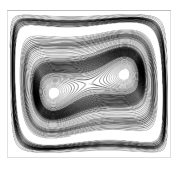
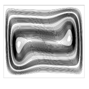
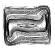
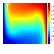
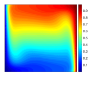
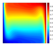
Figure 2: The resolved solution’s velocity streamlines (top) and temperature contours (bottom), for $Ra=10^{5}$, $Ra=5\cdot 10^{5}$, and $Ra=10^{6}$, from left to right.

We now demonstrate the Anderson accelerated Picard iteration for the Boussinesq system on a benchmark differentially heated cavity problem from [8], with varying Rayleigh number. The domain for the problem is the unit square, and for boundary conditions we enforce no slip velocity on all walls, $\nabla T\cdot n=0$ on the top and bottom, and $T(1,y)=1$, $T(0,y)=0$. The initial iterates $u_{0}=0$ and $T_{0}=0$, are used for all tests. No continuation method or pseudo time stepping is employed.

The discretization uses $(P_{2},P_{1}^{disc})$ velocity-pressure Scott-Vogelius elements, and $P_{2}$ temperature elements. The mesh is created by starting with a uniform triangulation, refining along the boundary, then applying a barycenter refinement (Alfeld split, in the language of Fu, Guzman and Neilan [13]). The resulting mesh is shown in figure 1, and with this element choice provides 89,554 total degrees of freedom. We show results below for varying Rayleigh numbers, which come from using parameters $\nu=0.01$ and $\kappa=0.01$, and varying $Ri$. Plots of resolved solutions for varying $Ra$ are shown in figure 2.

In our tests, we consider both constant algorithmic depts $m$, and also a 2-stage strategy that uses a smaller $m$ (1 or 2) when the nonlinear residual is larger than $10^{-3}$ in the B-norm, and $m=20$ when the residual is smaller. The 2-stage approach is motivated by Theorem 3.1, which suggests that greater depths $m$ can be detrimental early in the iteration due to the accumulation of non-negligible higher order terms in the residual expansion. Once the residual is sufficiently small, then the reduction of the first order terms from a greater depth $m$ can be enjoyed without noticeable pollution from the higher-order terms, which essentially results in an improved linear convergence rate.

$Ra=10^{5}$                                              $Ra=5\cdot 10^{5}$

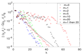
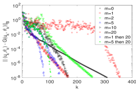
$Ra=10^{6}$                                              $Ra=2\cdot 10^{6}$

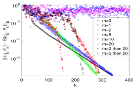
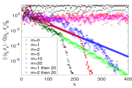
Figure 3: Convergence results for the differentially heated cavity with varying $m$, for several Rayleigh numbers.

We test here Algorithm 3.8, i.e. the Anderson accelerated Picard iteration for the Boussinesq system, for varying choices of depth $m$ and damping parameter $\beta$, and for several Rayleigh numbers: $Ra=10^{5},\ 5\cdot 10^{5},\ 10^{6},\ 2\cdot 10^{6}$. For each $Ra$, we tested with $m=0$ (no acceleration) and each fixed damping parameter $\beta=0.05,0.1,0.15,\ ...,1$, and then used the best $\beta$ from all tests with that $Ra$. Respectively, for $Ra=10^{5},\ 5\cdot 10^{5},\ 10^{6},\ 2\cdot 10^{6}$, these parameters were $\beta=0.3,\ 0.05,\ 0.05,\ 0.05$. Convergence results for varying $m$ are shown in figure 3, displayed in terms of the B-norm of the nonlinear residual versus iteration number. We note that the usual Picard iteration, i.e. $m=0$ and $\beta=1$, did not converge for any of these $Ra$ numbers; after 500 iterations, the B-norm was still larger than $10^{-1}$. With the appropriately chosen relaxation parameters, the Picard iteration did converge for each case except when $Ra=2\cdot 10^{6}$.

Convergence results for the lowest Rayleigh number, $Ra=10^{5}$, are shown in the top left of figure 3 for different values of $m$ and fixed $\beta=0.3$. Here, we observe the unaccelerated method converges rather quickly, and the accelerated methods that converged faster were $m=1$ and $m=2$ and the 2-stage method that uses $m=1$ and then switches to $m=20$, with the 2-stage method giving the best results. Anderson accelerated Picard with $m=5,\ 10,\ 20$ all converged, but slower than if no acceleration was used.

Results for $Ra=5\cdot 10^{5}$ also show lower values of $m$ improving convergence but higher values slowing convergence. Indeed, $m=1,2,5$ along with 2-stage methods that used $m=1$ then $20$ and $m=5$ then 20, all outperformed the unaccelerated iteration, while $m=10$ and $m=20$ slowed convergence. For $Ra=10^{6}$, the methods with smaller constant $m=1,2,5$ converged, all in roughly the same number of iterations as the unaccelerated method, while the methods run with larger $m=10,\ 20$ did not converge within 400 iterations. Once again, significant improvement is seen from using 2-stage choices of $m$, and this gave the best results.

With $Ra=2\cdot 10^{6}$, results showed more improvement from the acceleration, as compared to those with lower $Ra$. Here, the unaccelerated Picard iteration did not converge, and neither does the iteration with $m=1$. Again, the best results come from using a 2-stage choice of $m$, using a lesser depth at the beginning of the iteration, and a greater depth once the residual is sufficiently small.

The results described above show a clear advantage from using Anderson acceleration with the Picard iteration, especially for larger Rayleigh numbers. These results are also in good agreement with our theory

which demonstrates that Anderson acceleration decreases the first order term, but then adds higher order terms, to the residual bound. Hence using greater algorithmic depths when the residual is large can sufficiently pollute the solution so that the improvement found in the reduction of the first order term is outweighed by the additional contributions from higher order terms. In all cases, $m=10,\ 20$ slowed convergence compared to $m=0$, if the $m=0$ iteration converged. Both theory and these experiments also suggest that early in the iteration, moderate choices of algorithmic depth can be advantageous. The best results shown here come from the 2-stage strategy, which takes advantage of the reduction in the first-order residual term, but only once the residual is small enough that the higher-order contributions are negligible in comparison.

5 Acceleration of the Newton iteration for the Boussinesq system

While the theory for this paper focuses on the Picard iteration, it is also of interest to consider the Newton iteration for the Boussinesq system, which takes the form

$$(u_{k-1}\cdot\nabla)u_{k}+(u_{k}\cdot\nabla)u_{k-1}-(u_{k-1}\cdot\nabla)u_{k-1}-\nu\Delta u_{k}+\nabla p_{k} =Ri\langle 0,\theta_{k}\rangle^{T}+f,$$ (5.1)

$$\nabla\cdot u_{k} =0,$$ (5.2)

$$(u_{k-1}\cdot\nabla)\theta_{k}+(u_{k}\cdot\nabla)\theta_{k-1}-(u_{k-1}\cdot\nabla)\theta_{k-1}-\kappa\Delta\theta_{k} =\gamma,$$ (5.3)

together with appropriate boundary conditions.

The Newton iteration is often superior for solving nonlinear problems, particularly if one can find an initial guess sufficiently close to a solution. However, for Boussinesq systems, the Newton iteration also comes with a significant additional difficulty in that the linear systems that need to be solved at each iteration are fully coupled. That is, one needs to solve larger block linear systems for $(u_{k},p_{k},\theta_{k})$ simultaneously, whereas for the Picard iteration one first solves for $\theta_{k}$, and then solves a Navier-Stokes type system for $(u_{k},p_{k})$. Hence each iteration of Picard is significantly more efficient than each iteration of Newton.

We proceed now to test Anderson acceleration applied to the Newton iteration, using the same differentially heated cavity problem and discretization studied above. While theory to describe how Anderson acceleration can improve the performance of Newton iterations has yet to be developed, evidence for the efficacy of the method has been described in [10, 18]. While the acceleration can be expected to interfere with Newton’s quadratic convergence in the vicinity of a solulution, the advantage explored here is the behavior of the algorithm outside of that regime. In the far-field regime, outside the domain of asympotically quadratic convergence, the Newton iteration may converge linearly [19], or, of course, not at all. In comparing acccererated Newton with Newton augmented with a linesearch, we demonstrate how the acceleration can effectively enlarge the domain of convergence for Newton iterations. As shown in the experiments below, a damped accelerated Newton iteration with algorithmic depth $m=10$ can also solve the Boussinesq system with $Ra=2\cdot 10^{6}$.

In the following tests, convergence was declared if the nonlinear residual fell below $10^{-8}$ in the B-norm. If residuals grew larger than $10^{4}$ in the B-norm, the iteration was terminated, and the test was declared to fail due to (essentially) blowup, and is denoted with a ‘B’ in the tables below. If an iteration did not converge within 200 iterations but its residuals all stayed below $10^{4}$ in the B-norm, we declared it to be a failure and denote it with an ‘F’ in the tables below.

We first tested Anderson acceleration applied to the Newton iteration, with varying $m$ and no relaxation ($\beta=1$). Results are shown in table 1, and a clear improvement can be seen in convergence for higher $Ra$ as $m$ increases. For comparison, we also show results of (unaccelerated) Newton with a line search, and give results from two choices of line searches: LS1 continuously cuts the Newton step size ratio in half (up to 1/64), until either finding a step that decreases the nonlinear residual of the finite element problem, or using a step size ratio of 1/64 otherwise. LS2 uses ‘fminbnd’ from MATLAB (golden section search and parabolic interpolation) to use the step size ratio from [0.01,1] that minimizes the nonlinear residual of the finite element problem. While the line searches do help convergence of the Newton iteration, they do not perform as well as Newton-Anderson ($m=$5 or 10) for higher $Ra$ values.

$Ri$	$Ra$	$m=0$	$m=1$	$m=2$	$m=5$	$m=10$	$m=0$ + LS1	$m=0$ + LS2
1	1e+4	9	9	11	14	17	7	7
10	1e+5	B	17	19	81	38	B	11
20	2e+5	B	B	B	34	36	B	20
50	5e+5	B	B	B	44	56	B	B
100	1e+6	B	B	B	B	B	B	B
150	1.5e+6	B	B	B	B	B	B	B
200	2e+6	B	B	B	B	B	B	B

Table 1: Iterations required for Anderson accelerated Newton iterations to converge, with $\beta=1$ and varying $m$. Results of the unaccelerated Newton method with line searches are also shown.

We next considered Anderson acceleration to Newton, but using relaxation of $\beta=0.3$. Result are shown in table 2, and we observe further improvement compared to the case of $\beta=1$. Lastly, we considered Anderson acceleration applied to Newton, but choosing the $\beta$ from $\{0.0625,0.125,0.25,0.5,1\}$ that has the smallest residual in the B-norm. This is essentially a look-ahead step, which increases the cost of each step the accelerated Newton algorithm by a factor of 4. Results from choosing $\beta$ this way were significantly better than for constant $\beta=1$, and somewhat better than $\beta=0.3$, although not worth the extra cost except when using $\beta=0.3$ failed. A clear conclusion for this section is that Anderson acceleration with a properly chosen depth and relaxation can significantly improve the ability for the Newton iteration to converge for larger $Ra$.

$Ri$	$Ra$	$m=0$	$m=1$	$m=2$	$m=5$	$m=10$
1	1e+4	13	11	10	11	13
10	1e+5	B	18	18	23	52
20	2e+5	B	41	32	22	44
50	5e+5	B	B	B	74	134
100	1e+6	B	B	B	95	F
150	1.5e+6	B	B	B	B	141
200	2e+6	B	B	B	B	156

Table 2: Iterations required for Anderson acclerated Newton iterations to converge to a nonlinear residual of $10^{-8}$ in the B-norm, with $\beta=0.3$ and varying $m$. B denotes the nonlinear residual growing above $10^{4}$, and $F$ denotes no convergence after 200 iterations.

$Ri$	$Ra$	$m=0$	$m=1$	$m=2$	$m=5$	$m=10$
1	1e+4	8	9	9	13	24
10	1e+5	F	13	14	20	38
20	2e+5	123	21	27	32	61
50	5e+5	35	59	31	65	93
100	1e+6	B	42	F	68	106
150	1.5e+6	B	B	B	F	112
200	2e+6	B	B	B	F	150

Table 3: Iterations required for Anderson acclerated Newton iterations to converge to a nonlinear residual of $10^{-8}$ in the B-norm, with $\beta$ being chosen as the best from a set of five values, and varying $m$. B denotes the nonlinear residual growing above $10^{4}$, and $F$ denotes no convergence after 200 iteraitons.

6 Conclusions

In this paper, we studied Anderson acceleration applied to the Picard iteration for Boussinesq system. The Picard iteration is advantageous compared to the Newton iteration for this problem because it decouples the linear systems into easier to solve pieces. Since convergence of Picard iterations is typically slow, it is a good candidate for acceleration. In this work we showed that the Anderson acceleration analysis framework developed in [17] was applicable to this Picard iteration, by considering each iteration as the application of a particular solution operator, and then proving the solution operator had the required properties laid out in [17]. This in turn proved one-step error analysis results from [17] hold for Anderson acceleration applied to the Boussinesq system, and local convergence of the accelerated method under a small data condition. Numerical tests with the 2D differentially heated cavity problem showed good numerical results demonstrating the convergence behavior was consistent with our theory, and in particular that a 2-stage choice of Anderson depth works very well. Anderson acceleration applied to the related Newton iteration was also considered in numerical tests and it was found that Anderson acceleration allowed for convergence at significantly higher Rayleigh numbers than the usual Newton iteration with common line search techniques.

7 Acknowledgements

The author SP acknowledges support from National Science Foundation through the grant DMS 1852876.

References

- [1] M. Akbas, S. Kaya, and L. Rebholz. On the stability at all times of linearly extrapolated BDF2 timestepping for multiphysics incompressible flow problems. Num. Meth. P.D.E.s, 33(4):995–1017, 2017.
- [2] D. G. Anderson. Iterative procedures for nonlinear integral equations. J. Assoc. Comput. Mach., 12(4):547–560, 1965.
- [3] D. Arnold, F. Brezzi, and M. Fortin. A stable finite element for the Stokes equations. Calcolo, 21(4):337–344, 1984.
- [4] D. Arnold and J. Qin. Quadratic velocity/linear pressure Stokes elements. In R. Vichnevetsky, D. Knight, and G. Richter, editors, Advances in Computer Methods for Partial Differential Equations VII, pages 28–34. IMACS, 1992.
- [5] M. Benzi, G. Golub, and J. Liesen. Numerical solution of saddle point problems. Acta Numerica, 14:1–137, 2005.
- [6] M. Benzi and M. Olshanskii. An augmented Lagrangian-based approach to the Oseen problem. SIAM J. Sci. Comput., 28:2095–2113, 2006.
- [7] S. Brenner and L.R. Scott. The Mathematical Theory of Finite Element Methods, 3rd edition. Springer-Verlag, 2008.
- [8] A. Cibik and S. Kaya. A projection-based stabilized finite element method for steady state natural convection problem. Journal of Mathematical Analysis and Applications, 381:469–484, 2011.
- [9] H. Elman, D. Silvester, and A. Wathen. Finite Elements and Fast Iterative Solvers with applications in incompressible fluid dynamics. Numerical Mathematics and Scientific Computation. Oxford University Press, Oxford, 2014.
- [10] C. Evans, S. Pollock, L. Rebholz, and M. Xiao. A proof that anderson acceleration increases the convergence rate in linearly converging fixed point methods (but not in quadratically converging ones). SIAM Journal on Numerical Analysis, 58:788–810, 2020.
- [11] V. Eyert. A comparative study on methods for convergence acceleration of iterative vector sequences. J. Comput. Phys., 124(2):271–285, 1996.
- [12] H. Fang and Y. Saad. Two classes of multisecant methods for nonlinear acceleration. Numer. Linear Algebra Appl., 16(3):197–221, 2009.
- [13] G. Fu, J. Guzman, and M. Neilan. Exact smooth piecewise polynomial sequences on Alfeld splits. Mathematics of Computation, 89(323):1059–1091, 2020.
- [14] C.T. Kelley. Numerical methods for nonlinear equations. Acta Numerica, 27:207–287, 2018.
- [15] W. Layton. An Introduction to the Numerical Analysis of Viscous Incompressible Flows. SIAM, Philadelphia, 2008.
- [16] S. Pollock, L. Rebholz, and M. Xiao. Anderson-accelerated convergence of Picard iterations for incompressible Navier-Stokes equations. SIAM Journal on Numerical Analysis, 57(2):615– 637, 2019.
- [17] S. Pollock and L. G. Rebholz. Anderson acceleration for contractive and noncontractive iterations. Submitted, 2019.
- [18] S. Pollock and H. Schwartz. Benchmarking results for the Newton-Anderson method. Results in Applied Mathematics, in press, 2020.
- [19] V. Pták. The rate of convergence of Newton’s process. Numer. Math., 25:279–285, 1976.
- [20] A. Toth and C. T. Kelley. Convergence analysis for Anderson acceleration. SIAM J. Numer. Anal., 53(2):805–819, 2015.
- [21] H. F. Walker and P. Ni. Anderson acceleration for fixed-point iterations. SIAM J. Numer. Anal., 49(4):1715–1735, 2011.
- [22] S. Zhang. A new family of stable mixed finite elements for the 3d Stokes equations. Math. Comp., 74(250):543–554, 2005.
- [23] S. Zhang. A family of divergence-free finite elements on rectangular grids. SIAM J. Numer. Anal., 47(3):2090–2107, 2009.