Self6D: Self-Supervised Monocular 6D Object Pose Estimation

Abstract

6D object pose estimation is a fundamental problem in computer vision. Convolutional Neural Networks (CNNs) have recently proven to be capable of predicting reliable 6D pose estimates even from monocular images. Nonetheless, CNNs are identified as being extremely data-driven, and acquiring adequate annotations is oftentimes very time-consuming and labor intensive. To overcome this shortcoming, we propose the idea of monocular 6D pose estimation by means of self-supervised learning, removing the need for real annotations. After training our proposed network fully supervised with synthetic RGB data, we leverage recent advances in neural rendering to further self-supervise the model on unannotated real RGB-D data, seeking for a visually and geometrically optimal alignment. Extensive evaluations demonstrate that our proposed self-supervision is able to significantly enhance the model’s original performance, outperforming all other methods relying on synthetic data or employing elaborate techniques from the domain adaptation realm.

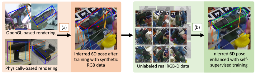
Figure 1: Abstract illustration of our proposed method. We visualize the 6D pose by overlaying the image with the corresponding transformed 3D bounding box. To circumvent the use of real 6D pose annotations, we firstly train our model purely on synthetic RGB data (a). Secondly, employing a large amount of unlabeled real RGB-D images (b), we significantly improve its performance (right). While Blue constitutes the ground truth pose, we demonstrate in Red and Green the results before and after applying our self-supervision, respectively.

1 Introduction

While learning-based techniques have recently demonstrated great performance in estimating the 6D pose (i.e. the 3D translation and rotation), a huge amount of training data is required [30, 44, 53]. Furthermore, contrary to most 2D computer vision tasks such as classification, object detection and segmentation, acquiring real world 6D object pose annotations is much more labor intensive, time consuming, and error-prone [13, 21].

In order to deal with the lack of real annotations, one common approach is to simulate a large amount of synthetic images [49, 51]. This is especially appealing for object pose estimation as one usually aims at estimating the 6D pose from an image w.r.t. the corresponding CAD model. Knowing the CAD model enables easy generation of enormous RGB images by randomly sampling 6D poses. Many approaches typically rely on rendering the models using OpenGL and placing them on random background images (drawn from large-scale 2D object datasets such as COCO [33]) in order to impose invariance to changing scenes [23, 40]. Recent works propose to instead employ physically-based rendering to produce high quality renderings, and additionally enforce real physical constraints, as they can provide additional cues for the 6D pose [16, 56].

Despite compelling results, these methods usually still exhibit inferior performance when inferring from real world data, due to the withstanding domain gap between real and synthetic data. Although techniques for domain adaption [2], domain randomization [52] and photorealistic rendering [16] can mitigate the problem to some extent, the performance is still far from satisfactory.

This motivated us to investigate the problem from an entirely different angle. Humans have the amazing ability to learn about the 3D world, whilst only perceiving it through 2D images. Moreover, they can even learn 3D world properties without supervision from another human or labels in a self-supervised fashion through making observations and validating if these observations are in accordance with the expected outcome [50]. In our context, while labeling the 6D pose is a severe bottleneck, recording unannotated data can be easily achieved at scale. Therefore, similar to learning for humans, we aim at teaching a neural network to reason about the 6D pose of an object by leveraging these unsupervised examples. As shown in Fig. 1, we first train our method fully-supervised with synthetic data. Afterwards, employing unannotaed RGB-D data, we make use of self-supervised learning to enhance the model’s performance on real data.

To accomplish this, it is required to understand 3D properties solely from 2D images. The mechanism of experiencing the 3D world as images on the eye’s retina is known as rendering and has been also extensively explored in Computer Graphics [41]. Unfortunately, rendering is also known to be non-differentiable due to the rasterization step, as gradients cannot be computed for the $argmax$ function. Nevertheless, many approaches for differentiable rendering have been recently proposed. The real gradient is thereby either approximated [22, 37], or computed analytically by approximating the rasterization function itself [35, 6].

In summary, we make the following contributions. i) To the best of our knowledge, we are the first to conduct self-supervised 6D object pose estimation from real data, without the need of 6D labels. ii) Leveraging neural rendering, we formulate a self-supervised 6D pose estimation solution by means of visual and geometric alignment. iii) We experimentally show that the proposed method, which we dub $\operatorname{Self6D}$, outperforms state-of-the-art methods for monocular 6D object pose estimation trained without real annotations by a large margin.

2 Related work

We first introduce recent work in monocular 6D pose estimation. Afterwards, we discuss important methods from neural rendering as they form a core part of our (as well as other) self-supervised learning frameworks. We then outline other successful approaches grounded on self-supervised learning. Lastly, we take a brief look at domain adaptation in the field of 6D pose, since our method can be considered an implicit formulation to close the synthetic-to-real domain gap.

2.1 Monocular 6D Pose Estimation

Recently, monocular 6D pose estimation has received a lot of attention and several very promising works have been proposed [15].

One major branch is grounded on establishing 2D-3D correspondences between the image and the 3D CAD model. After estimating these correspondences, P$n$P is commonly employed to solve for the 6D pose. Inspired by [3, 4], Rad et al. propose to employ a CNN to estimate the 2D projections of the 3D bounding box corners in image space [46]. Similarly, [17, 44] also regress 2D projections of associated sparse 3D keypoints, however, both employ segmentation paired with voting to improve the reliability. In contrast, [61, 30, 43] ascertain dense 2D-3D correspondences, rather than sparse ones.

Another branch of work learns a pose embedding, which can be utilized for latter retrieval. In particular, inspired by [58, 24], [52] employs an Augmented AutoEncoder (AAE) to learn latent representations for the 3D rotation.

A few methods also directly regress the 6D pose. For instance, while [23] extends [36] to also classify the viewpoint and in-plane rotation, [38] further adjusts [23] to implicitly deal with ambiguities via multiple hypotheses (MHP). In [59] and [29] the authors minimize a point matching loss.

The majority of these methods [17, 43, 46, 53, 59] exploit annotated real data to train their models. However, labeling real data commonly comes with a large cost in time and labor. Moreover, a shortage of sufficient real world annotations can lead to overfitting, regardless of exploiting strategies such as crop&paste [8, 21]. Other works, in contrast, fully rely on synthetic data to deal with these pitfalls [52, 38]. Nonetheless, the performance falls far behind the methods based on real data. We, thus, harness the best of both worlds. While unannotated data can be easily obtained at scale, this combined with our self-supervision for pose is able to outperform all methods trained on synthetic data by a large margin.

2.2 Neural Rendering

Rasterization is a core part of all traditional rendering pipelines. Nonetheless, rasterization involves discrete assignment operations, preventing the flow of gradients throughout the rendering process. A series of work have been devoted to circumvent the hard assignment in order to reestablish the gradient flow.

Loper and Black introduce the first differentiable renderer by means of first-order Taylor approximation to calculate the derivative of pixel values [37]. In [22], the authors instead approximate the gradient as the potential change of the pixel’s intensity w.r.t. the meshes’ vertices. SoftRas [35] conducts rendering by aggregating the probabilistic contributions of each mesh triangle in relation to the rendered pixels. Consequently, the gradients can be calculated analytically, however, with the cost of extra computation. DIB-R [6] further extends [35] to render of a variety of different lighting conditions. In this work, we use DIB-R [6] since it can be considered state-of-the-art for neural rendering.

2.3 Recent Trends in Self-Supervised Learning

Self-supervised learning, i.e. learning despite the lack of properly labeled data, has recently enabled a large number of applications ranging from 2D image understanding all the way down to depth estimation for autonomous driving. In the core, self-supervised learning approaches implicitly learn about a specific task through solving related proxy tasks. This is commonly achieved by enforcing different constraints such as pixel consistencies across multiple views or modalities.

One prominent approach in this area is MonoDepth [9], which conducts monocular depth estimation by warping the 2D image points into another view and enforcing a minimum reprojection loss. In the following many works to extend MonoDepth have been introduced [45, 10, 11]. In visual representation learning, consistency is ensured by solving pretext tasks [26]. Another line of works explore self-supervised learning for 3D human pose estimation, leveraging multi-view epipolar geometry [25] or imposing 2D-3D consistency after lifting and reprojection of keypoints [5]. Self-supervised learning approaches using neural rendering have also been proposed in the field of 3D object and human body reconstruction from single RGB images [57, 20, 42, 1, 64].

In the domain of 6D pose estimation, self-supervised learning is still a rather unexplored field. [7] proposes a novel self-labeling pipeline with an interactive robotic manipulator. Essentially, running several methods for 6D pose estimation, they can reliably generate precise annotations. Nonetheless, the final 6D pose estimation model is still trained fully-supervised using the acquired data. In this work, we propose to instead directly employ self-supervision for 6D pose by enforcing visual and geometric consistencies on top of neural rendering.

2.4 Domain Adaptation for 6D Pose Estimation

Bridging the domain gap between synthetic and real data is crucial in 6D pose estimation. Many works tackle this problem by learning a transformation to align the synthetic and real domains via Generative Adversarial Networks (GANs)  [2, 28] or by means of feature mapping [47]. Exemplary, [28] uses a cross-cycle consistency loss based on disentangled representations to embed images onto a domain-invariant content space and a domain-specific attribute space. [47] instead maps the features of a color-based pose estimator to a depth-based pose estimator.

In contrast, works from domain randomization aim at learning domain-invariant attributes. For instance, harnessing random backgrounds and severe augmentations [23, 52] or employing adversarial training to generate backgrounds and image augmentations [60].

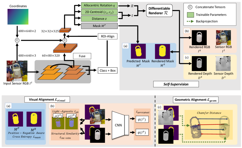
Figure 2: Our self-supervised training pipeline. Top: We start training our model for 6D pose estimation purely on synthetic RGB data, to predict a 3D rotation $R$, translation $t$ and object instance mask $M^{P}$. Using a large amount of unlabeled RGB-D images $(I^{S},D^{S})$, we enhance the model’s performance by means of self-supervised learning. We differentiably render ($\mathcal{R}$) the associated RGB-D image and mask $(I^{R},D^{R},M^{R})$. Bottom: We impose various constraints to visually (a and b), and geometrically (c) align the 6D pose.

3 Self-Supervised 6D Pose Estimation

In this work we aim at conducting 6D pose estimation from monocular images via self-supervised learning. To this end, we propose a novel model that can learn monocular pose estimation from both synthetic RGB data and real world unannotated RGB-D data. Employing neural rendering, the model can be self-supervised by establishing coherence between real and rendered images w.r.t. the 6D pose. Since this requires good initial pose estimates, we rely on a two-stage approach. As shown in Fig. 1, we start by training our model using synthetic RGB data only. Afterwards, we further enhance the pose estimation performance by leveraging unlabeled real world RGB-D data.

We harness different visual and geometric constraints to seek the best alignment w.r.t. 6D pose. Unfortunately, while a 3D model contains information about the visible and invisible regions, the depth map only covers the visible surface. This complicates supervision since the invisible points would mistakenly contribute to the alignment. Therefore, we aim to extract only the model’s visible surface given the current pose. This can be achieved in different ways: by culling the hidden points, or simply rendering the object in its current pose. Since we are required to render color for visual alignment, we resort to rendering depth for visible surface extraction, as it comes with no extra cost in computation.

We use the differentiable renderer DIB-R proposed by [6] to render 6D pose estimates from our model. Since DIB-R is only able to render RGB images and object masks, we extend it to also provide the depth map fully differentiably. We additionally modify the camera projection to conduct a real perspective projection . Given the estimated 6D pose as 3D rotation $R$, 3D translation $t$, together with the 3D CAD model $\mathcal{M}$ and the camera intrinsics matrix $K$, we render the triplet $(I^{R},D^{R},M^{R})$ consisting of the rendered RGB image $I^{R}$, the rendered depth map $D^{R}$ and the rendered mask $M^{R}$

$$\mathcal{R}(R,t,K,\mathcal{M})=(I^{R},D^{R},M^{R}).$$ (1)

Architecture Details.

Besides rendering, also the prediction of the 3D rotation and translation has to be differentiable in order to allow backpropagation. While methods based on establishing 2D-3D correspondences are currently dominating the field, it is infeasible to resort to them as gradients cannot be computed for P$n$P. To this end, we rely on a similar network architecture as ROI-10D [39], since they directly estimate rotation and translation. Unfortunately, the predicted poses from ROI-10D are not accurate enough to match the demands of our self-supervision, thus, we base our method on the more recent FCOS [54] detector. Moreover, a crucial part of our subsequent self-supervision requires object instance masks. Since no annotations are provided, we further extend ROI-10D to also estimate the visible object mask $M^{P}$ for each detection.

Our model is grounded on the object detector FCOS using a ResNet-50 based feature pyramid network (FPN) [31] backbone to compute 2D region proposals. The FPN feature maps from different levels are then fused and concatenated with the input RGB image and 2D coordinates [34], from which the regions of interest are extracted via ROI-Align to predict masks and poses. Inspired by ROI-10D, we use different branches to predict the 3D rotation $R$ parameterized as a 4D quaternion $q$, the 3D translation $t$ defined as the 2D projection $(c_{x},c_{y})$ of the 3D object centroid and the distance $z$, and the visible object mask $M^{P}$.

To train the first-stage, we use focal loss [32] for classification and GIoU loss [48] for bounding box regression. We rely on the binary cross entropy loss for mask prediction. As [29], we use the average of distinguishable model points metric as objective function for pose. The final loss can be summarized as

$$\mathcal{L}_{synthetic}\coloneqq\lambda_{class}\mathcal{L}_{focal}+\lambda_{box}\mathcal{L}_{giou}+\lambda_{mask}\mathcal{L}_{bce}+\lambda_{pose}\mathcal{L}_{pose},\quad$$ (2)

$$\text{with}\quad\mathcal{L}_{pose}\coloneqq\underset{x\in\mathcal{M}}{\operatorname{avg}}\|(R\mathbf{x}+t)-(\bar{R}\mathbf{x}+\bar{t})\|_{1},$$ (3)

where $\lambda_{class},\lambda_{box},\lambda_{mask}$ and $\lambda_{pose}$ denote the balance factors for each task, $\mathcal{M}$ denotes the 3D model, and $\left[R|t\right],\left[\bar{R}|\bar{t}\right]$ represent the predicted and ground truth poses, respectively. We kindly refer to the supplementary material for more details on the employed hyper-parameters.

For simplicity of the following, we define all foreground and background pixels as $N_{+}\coloneqq\{\,(i,j)\mid\forall M^{P}(i,j)=1\,\}$ and $N_{-}\coloneqq\{\,(i,j)\mid\forall M^{P}(i,j)=0\,\}$. We further denote all pixels together as $N=N_{+}\cup N_{-}$.

Neural Rendering for Visual Alignment.

The most intuitive way is to simply align the rendered image $I^{R}$ with the sensor image $I^{S}$, deploying directly a loss on both samples. However, as the domain gap between $I^{S}$ and $I^{R}$ turns out to be very large, this does not work well in practice. In particular, lightning changes as well as reflection and bad reconstruction quality (especially in terms of color) oftentimes cause a high error despite having good pose estimates, eventually leading to divergence in the optimization. Hence, in an effort to keep the domain gap as small as possible, we impose multiple constraints measuring different domain-independent properties. In particular, we assess different visual similarities w.r.t. mask, color, image structure, and high-level content.

Since object masks are naturally domain agnostic, they can provide a particularly strong supervision. As our data is unannotated we refer to our predicted masks $M^{P}$ for a weak supervision. However, due to imperfect predicted masks, we utilize a modified cross-entropy loss [18], which recalibrates the weights of positive and negative regions

$$\mathcal{L}_{mask}\coloneqq-\frac{1}{|N_{+}|}\sum_{j\in N_{+}}M_{j}^{P}\log M_{j}^{R}-\frac{1}{|N_{-}|}\sum_{j\in N_{-}}\log(1-M_{j}^{R}).$$ (4)

Although masks are not suffering from the domain gap, they discard a lot of valuable information. In particular, color information is often the only guidance to disambiguate the 6D pose, especially for geometrically simple objects.

Since the domain shift is at least partially caused by light, we attempt to decouple light prior to measuring color similarity. Let $\rho$ denote the transformation from RGB to LAB space, additionally discarding the light channel, we evaluate color coherence on the remaining two channels according to

$$\mathcal{L}_{ab}\coloneqq\frac{1}{|N_{+}|}\sum_{j\in N}\|\rho(I^{S})_{j}\cdot M_{j}^{P}-\rho(I^{R})_{j}\|_{1}.$$ (5)

We also avail various ideas from image reconstruction and domain translation, as they succumb the same dilemma. We assess the structural similarity (SSIM) in the RGB space and additionally follow the common practice to use a multi-scale variant, namely MS-SSIM [63]

$$\mathcal{L}_{ms\text{-}ssim}\coloneqq 1-ms\text{-}ssim(I^{S}\odot M^{P},I^{R},s).$$ (6)

Thereby, $\odot$ denotes the element-wise multiplication and $s=5$ is the number of employed scales. For more details on MS-SSIM, we kindly refer the readers to the supplement and [63].

Another common practice is to appraise the perceptual similarity [19, 62] in the feature space. To this end, a pretrained deep neural network as AlexNet [27] is typically employed to ensure low- and high-level similarity. We apply the perceptual loss at different levels of the CNN. Specifically, we extract the feature maps of $L=5$ layers and normalize them along the channel dimension. Then we compute squared $L_{2}$ distances of the normalized feature maps $\hat{\phi}^{l}(\cdot)$ for each layer $l$. We average the individual contributions spatially and sum across all layers [62]

$$\mathcal{L}_{perceptual}\coloneqq\sum_{l=1}^{L}\frac{1}{|N^{l}|}\sum_{j\in N^{l}}\|\hat{\phi}_{j}^{l}(I^{S}\odot M^{P})-\hat{\phi}_{j}^{l}(I^{R})\|_{2}^{2}.$$ (7)

The visual alignment is then composed as the weighted sum over all four terms

$$\mathcal{L}_{visual}\coloneqq\mathcal{L}_{mask}+\alpha\mathcal{L}_{ab}+\beta\mathcal{L}_{ms\text{-}ssim}+\gamma\mathcal{L}_{perceptual},$$ (8)

where $\alpha$, $\beta$ and $\gamma$ denote the balance factors for $\mathcal{L}_{ab}$, $\mathcal{L}_{ms\text{-}ssim}$, and $\mathcal{L}_{perceptual}$, respectively. We refer to the supplement for more details on the hyper-parameters.

Neural Rendering for Geometric Alignment.

Since the depth map only provides information for the visible areas, aligning it with the transformed 3D Model similar to Eq. 3 harms performance. Therefore, we exploit the rendered depth map to enable comparison of the visible areas only. Nevertheless, employing a loss directly on both depth maps leads to bad correspondences as the points where the masks are not intersecting cannot be matched.

Hence, we operate on the visible surface in 3D to find the best geometric alignment. We first backproject $D^{S}$ and $D^{R}$ using the corresponding masks $M^{P}$ and $M^{R}$ to retrieve the visible pointclouds $\mathcal{P}^{S}$ and $\mathcal{P}^{R}$ in camera space with

$$\pi^{-1}(D,M,K)=\{\,K^{-1}\begin{bmatrix}x_{j}&y_{j}&1\end{bmatrix}^{T}\cdot D_{j}\mid\forall j\in M>0\,\},$$ (9)

$$\mathcal{P}^{S}\coloneqq\pi^{-1}(D^{S},M^{P},K),\quad\quad\mathcal{P}^{R}\coloneqq\pi^{-1}(D^{R},M^{R},K).$$ (10)

Thereby, $(x_{j},y_{j})$ denotes the 2D pixel location of $j$ in $M$.

Since it is infeasible to estimate direct 3D-3D correspondences between $\mathcal{P}^{S}$ and $\mathcal{P}^{R}$, we refer to the chamfer distance to seek the best alignment in 3D

The overall self-supervision is $\mathcal{L}_{Self}\coloneqq\mathcal{L}_{visual}+\eta\mathcal{L}_{geom}$, with $\eta$ denoting the balance factor of $\mathcal{L}_{geom}$. An overview is also presented in Fig. 2. Noteworthy, while we require RGB-D data for self-supervision, we do not need any depth data during latter inference.

4 Evaluation

In this section, we first introduce our experimental setup. Afterwards, we present the analysis on the quality of predicted masks and different ablations to illustrate the effectiveness of our proposed self-supervised loss. We conclude by comparing our method with otherstate-of-the-art methods for 6D pose estimation and domain adaptation. For better understanding, in addition to the results of $\operatorname{Self6D}$, we also evaluate our method using synthetic data only and additionally employing real 6D pose labels. Since they can be considered the lower and upper bound of our method, we refer to them $\operatorname{Self6D-LB}$ and $\operatorname{Self6D-UB}$ in the following.

Synthetic Training Data.

[55] and [16] recently proposed to employ photorealistic and physically plausible renderings to improve 2D detection and 6D pose estimation, in contrast to simple OpenGL rendering [23]. In our experiments it turns out that a mixture of both approaches, together with a lot of augmentations (e.g. random Gaussian noise, intensity jitter), leads to best results.

Datasets.

To evaluate our proposed method we leverage the commonly used LineMOD dataset [12], which consists of 15 sequences, Only 13 of these provide water-tight CAD models and we, therefore, remove the other two sequences. In [3], the authors propose to sample $15\%$ of the real data for training to close the domain gap. We use the same split, however discarding the pose labels. As second dataset, we utilize the recent HomebrewedDB [21] dataset. However, we only employ the sequence which covers three objects from LineMOD, to depict that we can even self-supervise the same model in a new environment.

To also show generalization to other common datasets for 6D pose, we demonstrate the effectiveness of our self-supervision on 5 objects from YCB-Video [59] in the supplementary material. To compare with domain adaptation based methods, we refer to the usual Cropped LineMOD dataset [58] including center-cropped $64\times 64$ patches of 11 different small objects in cluttered scenes imaged in various of poses.

Metrics for 6D Pose.

We report our results w.r.t. the ADD metric [12], measuring whether the average deviation of the transformed model points is less than $10\%$ of the object’s diameter. For symmetric objects (e.g., Eggbox and Glue in LineMOD) we rely on the ADD-S metric, which instead measures the error as the average distance to the closest model point [12, 14].

$$\textbf{ADD}=\underset{x\in\mathcal{M}}{\operatorname{avg}}\|(Rx+t)-(\bar{R}x+\bar{t})\|_{2},$$ (12)

$$\textbf{ADD-S}=\underset{x_{2}\in\mathcal{M}}{\operatorname{avg}}\min_{x_{1}\in\mathcal{M}}\|(Rx_{1}+t)-(\bar{R}x_{2}+\bar{t})\|_{2}.$$ (13)

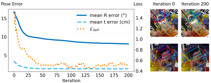
Figure 3: Pose errors v.s. self-supervision. We optimize $\mathcal{L}_{self}$ on single images from LineMOD for 200 iterations and report the average over in total 100 images. We initialize the 6D poses with $\operatorname{Self6D-LB}$.

4.1 Analysis on the Quality of Predicted Masks

Thanks to physically-based renderings, the predicted masks on the real data are very accurate, thus can be reliably used as a self-supervision signal. For instance, on the LineMOD test set, the average F1 score and mIoU between the predicted masks and the ground-truth masks are 89.63% and 90.38%. Please refer to the supplementary for detailed results and qualitative examples.

4.2 Ablation Study

Self-Supervision v.s. 6D Pose Error.

We want to demonstrate that there is indeed a high correlation between our proposed $\mathcal{L}_{Self}$ and the actual 6D pose errors. To this end, we randomly draw 100 samples from LineMOD and optimize separately on each sample, always beginning from $\operatorname{Self6D-LB}$. Fig. 3 illustrates the average behavior w.r.t. loss v.s.  6D pose error at each iteration. As the loss decreases, also the pose error for both, rotation and translation, continuously declines until convergence. The accompanying qualitative images (Fig. 3, right) further support this observation, as the initial pose is significantly worse compared to the final optimized result. We refer to the supplementary material for more qualitative results.

Individual Loss Contributions.

	Ape	Bvise	Cam	Can	Cat	Drill	Duck	Eggbox	Glue	Holep	Iron	Lamp	Phone	Mean
w/o $\mathcal{L}_{mask}$	0.0	0.0	0.0	0.0	0.0	0.0	0.0	0.8	0.0	0.0	0.0	0.0	0.0	0.1
w/o $\mathcal{L}_{geom}$	0.0	10.1	3.1	0.0	0.0	7.5	0.1	33.0	0.2	0.0	5.9	20.7	2.4	6.4
w/o $\mathcal{L}_{ms\text{-}ssim}$	32.1	74.8	20.4	63.4	57.1	68.3	16.6	99.0	94.1	12.3	70.8	68.5	54.9	56.3
w/o $\mathcal{L}_{perceptual}$	34.9	74.4	33.5	64.8	55.3	70.0	17.2	98.7	94.8	10.7	76.3	68.1	56.5	58.1
w/o $\mathcal{L}_{ab}$	40.9	73.8	36.1	63.0	58.1	66.0	18.0	98.9	93.9	16.2	77.2	68.2	50.1	58.5
$\operatorname{Self6D}$	38.9	75.2	36.9	65.6	57.9	67.0	19.6	99.0	94.1	15.5	77.9	68.2	50.1	58.9
$\operatorname{Self6D-LB}$	14.8	68.9	17.9	50.4	33.7	47.4	18.3	64.8	59.9	5.2	68.0	35.3	36.5	40.1
$\operatorname{Self6D-UB}$	62.3	95.3	86.5	93.0	80.7	93.7	63.4	99.7	99.4	73.6	96.0	96.6	90.0	86.9

Table 1: Ablation. We report the Average Recall of ADD(-S) on LineMOD.

Table 1 illustrates the contribution of each individual loss component on LineMOD. Note that supervision from both visual and geometry domains is vital for our self-supervised training. Disabling either $\mathcal{L}_{mask}$ or $\mathcal{L}_{geom}$ almost always leads to unstable training and divergence (the average recall is only $0.1\%$ and $6.4\%$ w.r.t. ADD(-S)). The remaining three factors, measuring color similarity, have a comparably small impact. Concretely, we drop by more than $2\%$ when disabling $\mathcal{L}_{ms\text{-}ssim}$, and about $1\%$ referring to $\mathcal{L}_{ab}$ and $\mathcal{L}_{perceptual}$. Nonetheless, we still achieve the overall best results when applying all loss terms together. Most importantly, we can report a significant relative improvement of almost $50\%$ from $40.1\%$ to $58.9\%$ leveraging the proposed self-supervision. Moreover, except for the Duck object, all other objects undergo a strong enhancement in ADD(-S). Noteworthy, we can almost halve the difference between training with and without real pose labels.

4.3 Comparison with State-of-the-art

In the first part of this section we present a comparison with current state-of-the-art methods in 6D pose estimation. In the latter part, we present our results in the area of domain adaptation referring to Cropped LineMOD.

4.3.1 6D Pose Estimation

LineMOD Dataset.

Train data	w/o Real Pose Labels				with Real Pose Labels
Object	AAE[52]	MHP[38]	DPOD[61]	$\operatorname{Self6D}$	Tekin[53]	DPOD[61]	PVNet[44]	CDPN[30]
Ape	4.0	11.9	35.1	38.9	21.6	53.3	43.6	64.4
Bvise	20.9	66.2	59.4	75.2	81.8	95.2	99.9	97.8
Cam	30.5	22.4	15.5	36.9	36.6	90.0	86.9	91.7
Can	35.9	59.8	48.8	65.6	68.8	94.1	95.5	95.9
Cat	17.9	26.9	28.1	57.9	41.8	60.4	79.3	83.8
Drill	24.0	44.6	59.3	67.0	63.5	97.4	96.4	96.2
Duck	4.9	8.3	25.6	19.6	27.2	66.0	52.6	66.8
Eggbox	81.0	55.7	51.2	99.0	69.6	99.6	99.2	99.7
Glue	45.5	54.6	34.6	94.1	80.0	93.8	95.7	99.6
Holep	17.6	15.5	17.7	16.2	42.6	64.9	81.9	85.8
Iron	32.0	60.8	84.7	77.9	75.0	99.8	98.9	97.9
Lamp	60.5	–	45.0	68.2	71.1	88.1	99.3	97.9
Phone	33.8	34.4	20.9	50.1	47.7	71.4	92.4	90.8
Mean	31.4	38.8	40.5	58.9	56.0	82.6	86.3	89.9

Table 2: Results for LineMOD. Top: Qualitative results. We depict the 6D pose by overlaying the 3D bounding box onto the input image. Blue constitutes the ground truth pose, red and green show our results before and after self-supervision. None of the samples has been seen before. Bottom: Comparison with state-of-the-art. We present the results for the Average Recall(%) of ADD(-S) metric. Real Pose Labels refers to the 15% training split from [3] with pose labels. We use the same split for training, however, without employing labels.

In line with other works, we distinguish between training with and without real pose labels, i.e. making use of annotated real training data. Despite exploiting real data, we do not employ any pose labels and must, therefore, be classified as the latter. We want to highlight that our model can produce state-of-the-art results for training with and without labels. Referring to Table 2, for training using only synthetic data, $\operatorname{Self6D-LB}$ reveals an average recall of $40.1\%$, which is deliberately better than AAE [52] with $31.4\%$ and on par with MHP [38] and DPOD [61] reporting $38.8\%$ and $40.5\%$. On the other hand, as for training with real pose labels, we are again on par with other recently published methods such as PVNet [44] and CDPN [30] reporting a mean average recall of $86.9\%$. Furthermore, our proposed self-supervision $\operatorname{Self6D}$ achieves an overall average recall of $58.9\%$, which is more than $51\%$ of relative improvement over all state-of-the-art methods using no real pose labels. Except for Holep, Duck and Iron, we can report a significant increase. Objects with little variation in color and geometry can become difficult to optimize. In addition, the 3D mesh of the Holep is rather different compared with the actual perceived object in the real images, which makes our visual alignment less meaningful.

HomebrewedDB Dataset.

Method	Supervision			Object
	Syn	Self	Real GT	Bvise	Driller	Phone	Mean
DPOD [61]	✓			52.9	37.8	7.3	32.7
SSD6D+Ref. [40]	✓			82.0	22.9	24.9	43.3
$\operatorname{Self6D-LB}$	✓			37.7	19.2	20.9	25.9
$\operatorname{Self6D}$	✓	✓		72.1	65.1	41.8	59.7
$\operatorname{Self6D-UB}$	✓		✓	71.0	64.2	46.5	60.6

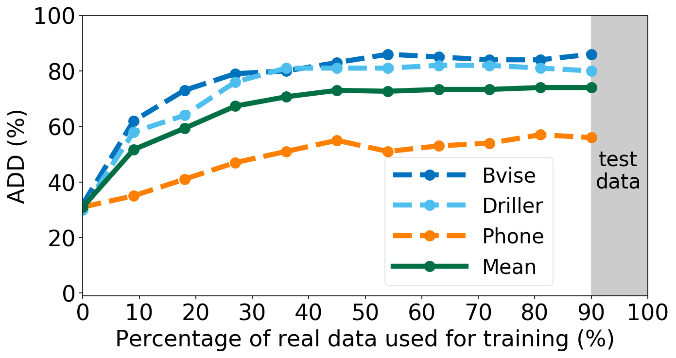
Figure 4: Results for HomebrewedDB. Left: Comparison with [61] and [40]. We report our results for synthetic data ($\operatorname{Self6D-LB}$) and after self-supervision ($\operatorname{Self6D}$) or full-supervision ($\operatorname{Self6D-UB}$) using 15% of real data from [21]. Right: Self-supervised training w.r.t. an increasing percentage of real training data. Results are always reported on the same unseen test split.

In Fig. 2 (left) we compare our method with DPOD [61] and SSD6D [23] after refinement using [40] (SSD6D+Ref.) on three objects of HomebrewedDB, which it shares with LineMOD. Unfortunately, methods directly solving for the 6D pose always implicitly learn the camera intrinsics which degrades the performance when exposed to a new camera. 2D-3D correspondences based approaches are instead robust to camera changes as they simply run P$n$P using the new intrinsics. Therefore, the performance of our $\operatorname{Self6D-LB}$ is slightly outperformed by [61]. SSD6D+Ref.  [40] employs contour-based pose refinement using renderings for the current hypotheses. Similarly, rendering the pose with the new intrinsics enables again easy adaptation and can even exceed [61] and our $\operatorname{Self6D}$ on the Bvise object. Nevertheless, we can easily adapt to the new domain and intrinsics by only leveraging 15% of unannotated data from [21]. In fact, we almost double their numbers for all other objects and reach a similar level as for LineMOD.

Based on this observation, we were curious to understand the adaptation capabilities of our model w.r.t. the amount of real data that we expose it to. We divided the samples from HomebrewedDB into 100 images for testing and 900 images for training. Afterwards, we repeatedly trained our model with increasing amount of data, however, always evaluating on the same test split. In Fig. 2 (right) we illustrate the corresponding results. When using only 15% (150 samples) of the real data for training, we can already almost double the mean average recall (mAR). Using $\approx$ 40% of the real data, the mAR can be improved by $\approx$ 130% from 31% to 71%. Afterwards, it slowly saturates at $\approx$ 74%.

LineMOD Occlusion Dataset.

Method	Supervision			Object
	Syn	Self	Real GT	Ape	Can	Cat	Driller	Duck	Eggbox	Glue	Holep	Mean
DPOD [61]	✓			2.3	4.0	1.2	10.5	7.2	4.4	12.9	7.5	6.3
CDPN [30]	✓			20.0	15.1	16.4	5.0	22.2	36.1	27.9	24.0	20.8
$\operatorname{Self6D-LB}$	✓			7.4	14.1	7.6	18.0	12.2	18.3	31.4	11.5	15.1
$\operatorname{Self6D}$	✓	✓		13.7	43.2	18.7	32.5	14.4	57.8	54.3	22.0	32.1
$\operatorname{Self6D-UB}$	✓		✓	47.4	79.4	56.1	83.5	48.9	90.0	93.6	62.5	70.2

Table 3: Results for LineMOD Occlusion. Comparison with [61] and [30]. We evaluate the Average Recall(%) of ADD(-S) on the BOP [15] split.

We also evaluate our method on LineMOD Occlusion which exhibits stronger occlusion. We follow the BOP [15] standard and evaluate on a subset of 200 samples. We compare $\operatorname{Self6D}$ with two state-of-the-art methods using synthetic data only, namely DPOD [61] and CDPN [30]. While our $\operatorname{Self6D-LB}$ can clearly outperform [61] with 15.1% compared to 6.3%, [30] exceeds our $\operatorname{Self6D-LB}$ by 5.4% and reports a mean average recall of 20.8%. 2D-3D correspondences based methods are more robust towards occlusion as they consider only the visible regions, while direct methods are less stable due to inferring poses from both visible and occluded regions. Nonetheless, after utilizing the remaining real RGB-D data via our self-supervision, we can easily surpass [30] (32.1% v.s. 20.8%), and double the performance of our $\operatorname{Self6D-LB}$. Noteworthy, there is still plenty of room for all the methods trained without real labels, compared to our fully-supervised model $\operatorname{Self6D-UB}$ (70.2%).

4.3.2 Domain Adaptation for Pose Estimation

Method	PixelDA [2]	DRIT [28]	DeceptionNet [60]	$\operatorname{Self6D-LB}$	$\operatorname{Self6D}$
Classification Accuracy (%)	99.9	98.1	95.8	100.0	100.0
Mean Angle Error (°)	23.5	34.4	51.9	19.8	15.8

Table 4: Comparison with state of the art on Cropped LineMOD. We present the classification accuracy as well as mean angle error.

Since our method is suitable for conducting synthetic to real domain adaptation, we assess transfer skills referring to the commonly used Cropped LineMOD scenario. We self-supervise the model with the real training set from Cropped LineMOD, and report the mean angle error on the real test set. As shown in Table 4, our synthetically trained model ($\operatorname{Self6D-LB}$) slightly exceeds state-of-the-art methods as PixelDA [2]. $\operatorname{Self6D}$ can successfully surpass the original model on the target domain, reducing the mean angle error from $19.8\degree$ to $15.8\degree$.

5 Conclusion

This work introduced $\operatorname{Self6D}$, the first self-supervised 6D object pose estimation approach aimed at learning from real data without the need for 6D pose annotations. Leveraging neural rendering, we are able to enforce several visual and geometrical constraints, resulting in a remarkable leap forward compared to other state-of-the-art methods. Moreover, $\operatorname{Self6D}$ demonstrated to notably reduce the gap with the state of the art for pose estimation with real pose labels.

A main future direction is exploring how to overcome the need for depth data during self-supervision. Another interesting aspect is to incorporate also 2D detections into self-supervision, as this allows backpropagating the loss in an end-to-end fashion throughout the entire network.

5.0.1 Acknowledgements

This work was supported by China Scholarship Council (CSC) Grant #201906210393. This work was also supported by the National Key R&D Program of China under Grant 2018AAA0102801.

Appendix 0.A Implementation Details

0.A.1 More Architecture Details

As mentioned in Section 3 of the main paper, we employ different lightweight branches to predict the following outputs from the fused FPN feature maps: the 3D rotation $R$ parameterized as a 4D quaternion $q$, the 3D translation $t$ constituted by the 2D projection $(c_{x},c_{y})$ of the 3D object centroid together with the distance $z$, and the visible object mask $M^{P}$.

For fusion of the FPN feature maps, we first apply a convolutional layer to reduce the dimension of each layer from 128 to 64, we then conduct bilinearly rescaling for each layer to make them spatially equal with the largest feature map (i.e., $60\times 80$). Finally, we concatenate all different levels to obtain the fused FPN feature map.

Each of our lightweight branches consists of 4 convolutional layers (except 2 for the 2D centroid) with Group Normalization wu2018groupA and Leaky ReLU xu2015empiricalA having a negative slope of $0.1$. The final output of each predictor is obtained by employing either a $3\times 3$ convolutional layer (mask) or a fully connected layer employed after flattening the output of forelast layer (centroid, distance and rotation).

In line with other works zakharov2019dpodA,manhardt2019roiA, we freeze the parameters in the first 3 stages of the backbone, to reduce the risk of overfitting to synthetic data. We additionally apply various augmentations to the training RGB images, similar to sundermeyer2018implicitA,kehl2017ssdA.

0.A.2 Experimental Setup

We implemented our method in PyTorch 1.3 paszke2019pytorchA and ran all our experiments on a NVIDIA TitanX GPU. In the first stage, we trained our model with a batch size of 12 for 8 epochs. During self-supervision, we trained the model for another 100 epochs with a batch size of 3. We utilized RAdam liu2019radamA combined with Lookahead zhang2019lookahead for optimization. The initial learning rate was set to $10^{-4}$ and decayed after $72\%$ of the training phase using a cosine schedule loshchilov-ICLR17SGDRA.

0.A.2.1 Employed Hyper-Parameters for Losses.

Table 5 shows the employed hyper-parameters for training with synthetic data

$$\mathcal{L}_{synthetic}\coloneqq\lambda_{class}\mathcal{L}_{focal}+\lambda_{box}\mathcal{L}_{giou}+\lambda_{mask}\mathcal{L}_{bce}+\lambda_{pose}\mathcal{L}_{pose},$$ (14)

and self-supervised training on real data

$$\mathcal{L}_{Self}=\mathcal{L}_{visual}+\eta\mathcal{L}_{geom},$$ (15)

with

$$\mathcal{L}_{visual}=\mathcal{L}_{mask}+\alpha\mathcal{L}_{ab}+\beta\mathcal{L}_{ms\text{-}ssim}+\gamma\mathcal{L}_{perceptual}.$$ (16)

The hyper-parameters are empirically chosen to level the different loss contributions.

hyper-parameter	$\lambda_{class}$	$\lambda_{box}$	$\lambda_{mask}$	$\lambda_{pose}$	$\alpha$	$\beta$	$\gamma$	$\eta$
value	1.0	1.0	1.0	10.0	0.2	1.0	0.15	100

Table 5: Employed hyper-parameters for losses.

0.A.3 Details of $\mathcal{L}_{ms\text{-}ssim}$

In this section, we present the details of MS-SSIM loss ($\mathcal{L}_{ms\text{-}ssim}$), which is an important part for the visual alignment ($\mathcal{L}_{visual}$) referring to our proposed self-supervision ($\mathcal{L}_{Self}$). The structural similarity index (SSIM)  wang2004ssimA for pixel $p$ is defined as

$$ssim(p)=\frac{2\mu_{x}\mu_{y}+c_{1}}{\mu_{x}^{2}+\mu_{y}^{2}+c_{1}}\cdot\frac{2\sigma_{xy}+c_{2}}{\sigma_{x}^{2}+\sigma_{y}^{2}+c_{2}}=l(p)\cdot cs(p).$$ (17)

Thereby, SSIM is computed on blocks, with $(\mu_{x},\mu_{y})$ and $\big{(}\begin{smallmatrix}\sigma_{x}^{2}&\sigma_{xy}\\ \sigma_{xy}&\sigma_{y}^{2}\end{smallmatrix}\big{)}$ denoting the corresponding means and covariance matrix w.r.t. $p$, respectively. In practice, we employ two constants $c_{1}=0.01$ and $c_{2}=0.03$ for numerical stability. In zhao2016lossA, the authors extend this measurement to a perceptually-motivated loss function referring to a widely used multi-scale version of SSIM, namely MS-SSIM. Given a dyadic pyramid of $s$ levels, MS-SSIM can be written as

$$ms\text{-}ssim(p)=l_{s}^{\alpha}(p)\cdot\prod_{j=1}^{s}cs_{j}^{\beta_{j}}(p),$$ (18)

where $l_{s}$ and $cs_{j}$ are the functions defined on the right in Eq. (17) at scale $s$ and $j$, respectively. As in zhao2016lossA, we set $\alpha=1$, $\beta_{j}=1$, $\forall j\in\{1,...,s\}$, and $s=5$. For convenience, given two RGB images $I_{A}$ and $I_{B}$, we denote the MS-SSIM between them as $ms\text{-}ssim(I_{A},I_{B},s)$. Since, $ms\text{-}ssim$ measure the similarity between two samples with 1 being the maximum, we rewrite the MS-SSIM loss as

$$\mathcal{L}_{ms\text{-}ssim}\coloneqq 1-ms\text{-}ssim(I_{A},I_{B},s).$$ (19)

Appendix 0.B Detailed Analysis on the Quality of Predicted Masks

	Ape	Bvise	Cam	Can	Cat	Drill	Duck	Eggbox	Glue	Holep	Iron	Lamp	Phone	Mean
F1 score	94.44	92.04	81.57	92.51	91.60	91.51	92.17	94.82	89.57	91.02	91.31	78.16	84.52	89.63
IoU	94.72	92.45	83.41	92.88	92.08	92.03	93.76	95.02	90.35	91.90	91.80	79.13	85.39	90.38

Table 6: Detailed evaluation of predicted masks. We report the F1 score(%) and IoU(%) on LineMOD test set.

Since our self-supervision relies on high quality of the predicted masks from our synthetically trained model $\operatorname{Self6D-LB}$, we present the detailed quantitative evaluation in Table 6. Specifically, we calculated F1 score and IoU between the predicted masks and the ground-truth masks on LineMOD test set. We can see that the predicted masks are very accurate on almost all objects, with the average F1 score 89.63% and mIoU 90.38%. Thus we can regard the predicted masks from $\operatorname{Self6D-LB}$ as a reliable self-supervision signal. Fig. 5 shows some qualitative examples for the predicted masks on LineMOD test set.

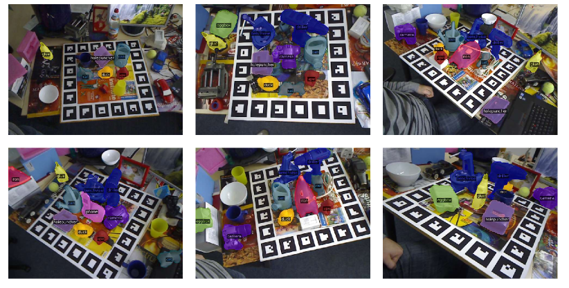
Figure 5: Qualitative results for predicted masks on LineMOD test set. (Best viewed zoomed-in, in color).

Appendix 0.C More Qualitative Results

In this section, we want to present additional qualitative results for each conducted experiment.

Domain Adaption. In Fig. 6, we demonstrate our results for domain adaption, leveraging the Cropped LineMOD dataset wohlhart2015learningA. While we constitute the ground truth poses in Blue, we demonstrate in Red and Green the results before (Self-LB) and after applying our self-supervision ($\operatorname{Self6D}$), respectively.

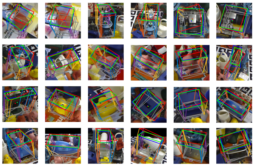
Figure 6: Qualitative results on Cropped LineMOD. We visualize the 6D pose by overlaying the image with the corresponding transformed 3D bounding box. While Blue constitutes the ground truth pose, we demonstrate in Red and Green the results before and after applying our self-supervision, respectively.

6D Pose Estimation We additionally present qualitative results for 6D pose estimation. Notice that we again depict the ground truth pose in Blue and the prediction before ($\operatorname{Self6D-LB}$) and after self-supervision ($\operatorname{Self6D}$) in Red and Green. While the initial results are very noisy in terms of 6D pose, the self-supervised model produces highly accurate pose estimates w.r.t. the given ground truth.

The results on LineMOD Occlusion Brachmann2014Learning6OA, HomebrewedDB kaskman2019homebreweddbA, and LineMOD Hinterstoisser2012A are respectively depicted in Fig. 7, Fig. 8, and Fig. 9.

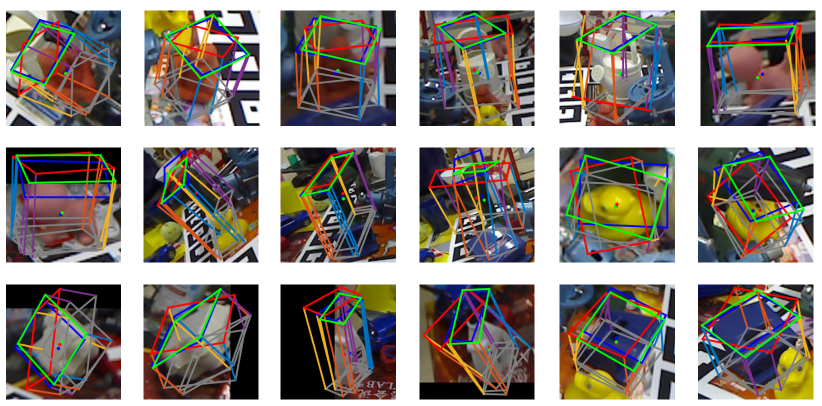
Figure 7: Qualitative results on LineMOD Occlusion. We visualize the 6D pose by overlaying the image with the corresponding transformed 3D bounding box. While Blue constitutes the ground truth pose, we demonstrate in Red and Green the results before and after applying our self-supervision, respectively.

Figure 8: Qualitative results on HomebrewedDB. We visualize the 6D pose by overlaying the image with the corresponding transformed 3D bounding box. While Blue constitutes the ground truth pose, we demonstrate in Red and Green the results before and after applying our self-supervision, respectively.

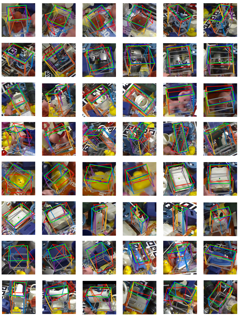
Figure 9: More qualitative results on LineMOD. We visualize the 6D pose by overlaying the image with the corresponding transformed 3D bounding box. While Blue constitutes the ground truth pose, we demonstrate in Red and Green the results before and after applying our self-supervision, respectively.

Self-Supervision v.s.  6D Pose Error. In the main paper, we demonstrate the existence of a strong correlation between our self-supervised loss function and the 6D pose accuracy. In particular, we conduct our self-supervision separately to single images for in total 200 iterations. In Fig. 10, we illustrate additional qualitative results for this experiment. Despite not possessing any pose labels, we can always compute pose estimates (Green) which are almost perfectly aligned with the ground truth (Blue). This is even true for poses, which are badly initialized using $\operatorname{Self6D-LB}$ (Red). This strongly suggest that our loss function is able to solve for the 6D pose, while actually optimizing for visual and geometric alignment.

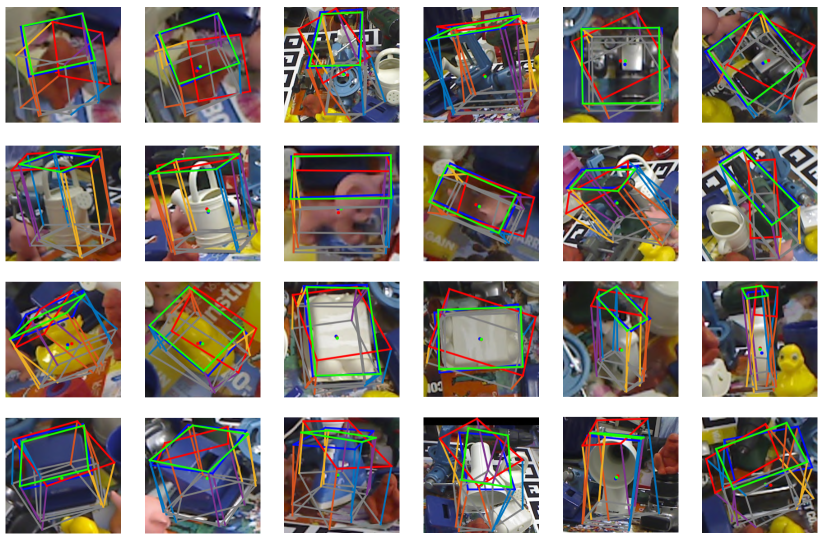
Figure 10: More qualitative results on Self-Supervision v.s.  6D Pose Error. We visualize the 6D pose by overlaying the image with the corresponding transformed 3D bounding box. While Blue constitutes the ground truth pose, we demonstrate in Red and Green the results before and after applying our self-supervision to the single image for 200 iterations, respectively.

Appendix 0.D Results on YCB-Video

	$\operatorname{Self6D-LB}$	$\operatorname{Self6D}$
006_mustard_bottle	73.7	88.2
007_tuna_fish_can	26.6	69.7
011_banana	4.0	10.3
025_mug	23.9	43.4
035_power_drill	21.4	31.4
Mean	29.9	48.6

Table 7: Left: Results on YCB-Video xiang2017posecnnA dataset. We report Average Recall (%) of ADD-S for the top 4 objects and ADD for 035_power_drill. Right: Qualitative results.

Although being out of the scope for the main body of this work, we further evaluated our method on a subset (5 objects) of YCB-Video xiang2017posecnnA, in order to emphasize that $\operatorname{Self6D}$ can be applied to any 6D pose scenario.

We first fully supervise $\operatorname{Self6D-LB}$ on a mixture of synthetic RGB images from YCB-Video and photorealistic renderings from tremblay2018fallingA. We then self-supervise the model on 10% of the real RGB-D images for each of these 5 objects from the training set, however, without leveraging any 6D annotations ($\operatorname{Self6D}$). Since the first four objects exhibit rotational symmetries, we report the average recall for ADD-S for them. For the remaining object (i.e. 035_power_drill), we refer to ADD instead, as it does not possess rotational symmetries. In line with all other experiments, we can constitute that leveraging our self-supervision, we are able to significantly enhance the average recall w.r.t. ADD(-S) for each object (Table 7).

splncs04 egbib

References

- [1] Alldieck, T., Magnor, M., Bhatnagar, B.L., Theobalt, C., Pons-Moll, G.: Learning to reconstruct people in clothing from a single rgb camera. In: CVPR. pp. 1175–1186 (2019)
- [2] Bousmalis, K., Silberman, N., Dohan, D., Erhan, D., Krishnan, D.: Unsupervised pixel-level domain adaptation with generative adversarial networks. In: IEEE Conference on Computer Vision and Pattern Recognition (CVPR). pp. 3722–3731 (2017)
- [3] Brachmann, E., Krull, A., Michel, F., Gumhold, S., Shotton, J., Rother, C.: Learning 6D object pose estimation using 3D object coordinates. In: European Conference on Computer Vision (ECCV). pp. 536–551 (2014)
- [4] Brachmann, E., Michel, F., Krull, A., Ying Yang, M., Gumhold, S., Rother, C.: Uncertainty-driven 6D pose estimation of objects and scenes from a single RGB image. In: IEEE Conference on Computer Vision and Pattern Recognition (CVPR). pp. 3364–3372 (2016)
- [5] Chen, C.H., Tyagi, A., Agrawal, A., Drover, D., Stojanov, S., Rehg, J.M.: Unsupervised 3d pose estimation with geometric self-supervision. In: IEEE Conference on Computer Vision and Pattern Recognition (CVPR). pp. 5714–5724 (2019)
- [6] Chen, W., Ling, H., Gao, J., Smith, E., Lehtinen, J., Jacobson, A., Fidler, S.: Learning to predict 3d objects with an interpolation-based differentiable renderer. In: Advances in Neural Information Processing Systems (NeurIPS). pp. 9605–9616 (2019)
- [7] Deng, X., Xiang, Y., Mousavian, A., Eppner, C., Bretl, T., Fox, D.: Self-supervised 6d object pose estimation for robot manipulation. In: IEEE International Conference on Robotics and Automation (ICRA) (2020)
- [8] Dwibedi, D., Misra, I., Hebert, M.: Cut, paste and learn: Surprisingly easy synthesis for instance detection. In: IEEE International Conference on Computer Vision (ICCV). pp. 1301–1310 (2017)
- [9] Godard, C., Mac Aodha, O., Brostow, G.J.: Unsupervised monocular depth estimation with left-right consistency. In: IEEE Conference on Computer Vision and Pattern Recognition (CVPR). pp. 270–279 (2017)
- [10] Godard, C., Mac Aodha, O., Firman, M., Brostow, G.J.: Digging into self-supervised monocular depth estimation. In: IEEE International Conference on Computer Vision (ICCV). pp. 3828–3838 (2019)
- [11] Guizilini, V., Ambrus, R., Pillai, S., Raventos, A., Gaidon, A.: 3d packing for self-supervised monocular depth estimation. In: CVPR (June 2020)
- [12] Hinterstoisser, S., Lepetit, V., Ilic, S., Holzer, S., Bradski, G., Konolige, K., Navab, N.: Model based training, detection and pose estimation of texture-less 3d objects in heavily cluttered scenes. In: Asian Conference on Computer Vision (ACCV). pp. 548–562 (2012)
- [13] Hodan, T., Haluza, P., Obdržálek, Š., Matas, J., Lourakis, M., Zabulis, X.: T-less: An rgb-d dataset for 6d pose estimation of texture-less objects. In: IEEE Winter Conference on Applications of Computer Vision (WACV). pp. 880–888 (2017)
- [14] Hodaň, T., Matas, J., Obdržálek, Š.: On evaluation of 6d object pose estimation. European Conference on Computer Vision Workshops (ECCVW) pp. 606–619 (2016)
- [15] Hodan, T., Michel, F., Brachmann, E., Kehl, W., GlentBuch, A., Kraft, D., Drost, B., Vidal, J., Ihrke, S., Zabulis, X., et al.: BOP: Benchmark for 6d object pose estimation. In: European Conference on Computer Vision (ECCV). pp. 19–34 (2018)
- [16] Hodaň, T., Vineet, V., Gal, R., Shalev, E., Hanzelka, J., Connell, T., Urbina, P., Sinha, S., Guenter, B.: Photorealistic image synthesis for object instance detection. IEEE International Conference on Image Processing (ICIP) (2019)
- [17] Hu, Y., Hugonot, J., Fua, P., Salzmann, M.: Segmentation-driven 6d object pose estimation. In: IEEE Conference on Computer Vision and Pattern Recognition (CVPR). pp. 3385–3394 (2019)
- [18] Jiang, P.T., Hou, Q., Cao, Y., Cheng, M.M., Wei, Y., Xiong, H.K.: Integral object mining via online attention accumulation. In: IEEE International Conference on Computer Vision (ICCV). pp. 2070–2079 (2019)
- [19] Johnson, J., Alahi, A., Fei-Fei, L.: Perceptual losses for real-time style transfer and super-resolution. In: European Conference on Computer Vision (ECCV). pp. 694–711 (2016)
- [20] Kanazawa, A., Tulsiani, S., Efros, A.A., Malik, J.: Learning category-specific mesh reconstruction from image collections. In: European Conference on Computer Vision (ECCV). pp. 371–386 (2018)
- [21] Kaskman, R., Zakharov, S., Shugurov, I., Ilic, S.: HomebrewedDB: RGB-D dataset for 6d pose estimation of 3d objects. In: IEEE International Conference on Computer Vision Workshops (ICCVW) (2019)
- [22] Kato, H., Ushiku, Y., Harada, T.: Neural 3d mesh renderer. In: IEEE Conference on Computer Vision and Pattern Recognition (CVPR). pp. 3907–3916 (2018)
- [23] Kehl, W., Manhardt, F., Tombari, F., Ilic, S., Navab, N.: Ssd-6d: Making rgb-based 3d detection and 6d pose estimation great again. In: IEEE International Conference on Computer Vision (ICCV). pp. 1521–1529 (2017)
- [24] Kehl, W., Milletari, F., Tombari, F., Ilic, S., Navab, N.: Deep learning of local RGB-D patches for 3D object detection and 6D pose estimation. In: European Conference on Computer Vision (ECCV). pp. 205–220 (2016)
- [25] Kocabas, M., Karagoz, S., Akbas, E.: Self-supervised learning of 3d human pose using multi-view geometry. In: IEEE Conference on Computer Vision and Pattern Recognition (CVPR). pp. 1077–1086 (2019)
- [26] Kolesnikov, A., Zhai, X., Beyer, L.: Revisiting self-supervised visual representation learning. In: IEEE Conference on Computer Vision and Pattern Recognition (CVPR). pp. 1920–1929 (2019)
- [27] Krizhevsky, A., Sutskever, I., Hinton, G.E.: Imagenet classification with deep convolutional neural networks. In: Advances in Neural Information Processing Systems (NeurIPS). pp. 1097–1105 (2012)
- [28] Lee, H.Y., Tseng, H.Y., Huang, J.B., Singh, M., Yang, M.H.: Diverse image-to-image translation via disentangled representations. In: European Conference on Computer Vision (ECCV). pp. 35–51 (2018)
- [29] Li, Y., Wang, G., Ji, X., Xiang, Y., Fox, D.: DeepIM: Deep iterative matching for 6d pose estimation. International Journal of Computer Vision (IJCV) pp. 1–22 (2019)
- [30] Li, Z., Wang, G., Ji, X.: CDPN: Coordinates-Based Disentangled Pose Network for Real-Time RGB-Based 6-DoF Object Pose Estimation. In: IEEE International Conference on Computer Vision (ICCV). pp. 7678–7687 (2019)
- [31] Lin, T.Y., Dollár, P., Girshick, R., He, K., Hariharan, B., Belongie, S.: Feature pyramid networks for object detection. In: IEEE Conference on Computer Vision and Pattern Recognition (CVPR). pp. 2117–2125 (2017)
- [32] Lin, T.Y., Goyal, P., Girshick, R., He, K., Dollar, P.: Focal loss for dense object detection. In: IEEE International Conference on Computer Vision (ICCV) (2017)
- [33] Lin, T.Y., Maire, M., Belongie, S., Hays, J., Perona, P., Ramanan, D., Dollár, P., Zitnick, C.L.: Microsoft coco: Common objects in context. In: European Conference on Computer Vision (ECCV). pp. 740–755 (2014)
- [34] Liu, R., Lehman, J., Molino, P., Such, F.P., Frank, E., Sergeev, A., Yosinski, J.: An intriguing failing of convolutional neural networks and the coordconv solution. In: Advances in Neural Information Processing Systems (NeurIPS). pp. 9605–9616 (2018)
- [35] Liu, S., Li, T., Chen, W., Li, H.: Soft rasterizer: A differentiable renderer for image-based 3d reasoning. IEEE International Conference on Computer Vision (ICCV) pp. 7708–7717 (2019)
- [36] Liu, W., Anguelov, D., Erhan, D., Szegedy, C., Reed, S., Fu, C.Y., Berg, A.C.: SSD: Single shot multibox detector. In: European Conference on Computer Vision (ECCV). pp. 21–37 (2016)
- [37] Loper, M.M., Black, M.J.: OpenDR: An approximate differentiable renderer. In: European Conference on Computer Vision (ECCV). vol. 8695, pp. 154–169 (2014)
- [38] Manhardt, F., Arroyo, D., Rupprecht, C., Busam, B., Birdal, T., Navab, N., Tombari, F.: Explaining the ambiguity of object detection and 6d pose from visual data. In: IEEE International Conference on Computer Vision (ICCV). pp. 6841–6850 (2019)
- [39] Manhardt, F., Kehl, W., Gaidon, A.: ROI-10D: Monocular lifting of 2d detection to 6d pose and metric shape. In: IEEE Conference on Computer Vision and Pattern Recognition (CVPR). pp. 2069–2078 (2019)
- [40] Manhardt, F., Kehl, W., Navab, N., Tombari, F.: Deep model-based 6d pose refinement in rgb. In: European Conference on Computer Vision (ECCV). pp. 800–815 (2018)
- [41] Marschner, S., Shirley, P.: Fundamentals of computer graphics. CRC Press (2015)
- [42] Omran, M., Lassner, C., Pons-Moll, G., Gehler, P., Schiele, B.: Neural body fitting: Unifying deep learning and model based human pose and shape estimation. In: 3DV. pp. 484–494 (2018)
- [43] Park, K., Patten, T., Vincze, M.: Pix2pose: Pixel-wise coordinate regression of objects for 6d pose estimation. In: IEEE International Conference on Computer Vision (ICCV). pp. 7668–7677 (2019)
- [44] Peng, S., Liu, Y., Huang, Q., Zhou, X., Bao, H.: Pvnet: Pixel-wise voting network for 6dof pose estimation. In: IEEE Conference on Computer Vision and Pattern Recognition (CVPR). pp. 4561–4570 (2019)
- [45] Pillai, S., Ambruş, R., Gaidon, A.: Superdepth: Self-supervised, super-resolved monocular depth estimation. In: IEEE International Conference on Robotics and Automation (ICRA). pp. 9250–9256 (2019)
- [46] Rad, M., Lepetit, V.: BB8: A scalable, accurate, robust to partial occlusion method for predicting the 3D poses of challenging objects without using depth. In: IEEE International Conference on Computer Vision (ICCV). pp. 3828–3836 (2017)
- [47] Rad, M., Oberweger, M., Lepetit, V.: Domain transfer for 3d pose estimation from color images without manual annotations. In: ACCV. pp. 69–84 (2018)
- [48] Rezatofighi, H., Tsoi, N., Gwak, J., Sadeghian, A., Reid, I., Savarese, S.: Generalized intersection over union: A metric and a loss for bounding box regression. In: IEEE Conference on Computer Vision and Pattern Recognition (CVPR). pp. 658–666 (2019)
- [49] Richter, S.R., Vineet, V., Roth, S., Koltun, V.: Playing for data: Ground truth from computer games. In: European Conference on Computer Vision (ECCV). pp. 102–118 (2016)
- [50] Spelke, E.S.: Principles of object perception. Cognitive science 14(1), 29–56 (1990)
- [51] Su, H., Qi, C.R., Li, Y., Guibas, L.J.: Render for cnn: Viewpoint estimation in images using cnns trained with rendered 3d model views. In: IEEE International Conference on Computer Vision (ICCV). pp. 2686–2694 (2015)
- [52] Sundermeyer, M., Marton, Z.C., Durner, M., Brucker, M., Triebel, R.: Implicit 3d orientation learning for 6d object detection from rgb images. In: European Conference on Computer Vision (ECCV). pp. 699–715 (2018)
- [53] Tekin, B., Sinha, S.N., Fua, P.: Real-Time Seamless Single Shot 6D Object Pose Prediction. In: IEEE Conference on Computer Vision and Pattern Recognition (CVPR). pp. 292–301 (2018)
- [54] Tian, Z., Shen, C., Chen, H., He, T.: FCOS: Fully convolutional one-stage object detection. In: IEEE International Conference on Computer Vision (ICCV). pp. 9627–9636 (2019)
- [55] Tremblay, J., To, T., Birchfield, S.: Falling things: A synthetic dataset for 3d object detection and pose estimation. In: IEEE Conference on Computer Vision and Pattern Recognition Workshops (CVPRW). pp. 2038–2041 (2018)
- [56] Tremblay, J., To, T., Sundaralingam, B., Xiang, Y., Fox, D., Birchfield, S.: Deep object pose estimation for semantic robotic grasping of household objects. In: Conference on Robot Learning (CoRL). pp. 306–316 (2018)
- [57] Tung, H.Y., Tung, H.W., Yumer, E., Fragkiadaki, K.: Self-supervised learning of motion capture. In: NeurIPS. pp. 5236–5246 (2017)
- [58] Wohlhart, P., Lepetit, V.: Learning descriptors for object recognition and 3d pose estimation. In: IEEE Conference on Computer Vision and Pattern Recognition (CVPR). pp. 3109–3118 (2015)
- [59] Xiang, Y., Schmidt, T., Narayanan, V., Fox, D.: PoseCNN: A convolutional neural network for 6D object pose estimation in cluttered scenes. Robotics: Science and Systems (RSS) (2018)
- [60] Zakharov, S., Kehl, W., Ilic, S.: Deceptionnet: Network-driven domain randomization. In: IEEE International Conference on Computer Vision (ICCV). pp. 532–541 (2019)
- [61] Zakharov, S., Shugurov, I., Ilic, S.: Dpod: 6d pose object detector and refiner. In: IEEE International Conference on Computer Vision (ICCV). pp. 1941–1950 (2019)
- [62] Zhang, R., Isola, P., Efros, A.A., Shechtman, E., Wang, O.: The unreasonable effectiveness of deep features as a perceptual metric. In: IEEE Conference on Computer Vision and Pattern Recognition (CVPR). pp. 586–595 (2018)
- [63] Zhao, H., Gallo, O., Frosio, I., Kautz, J.: Loss functions for image restoration with neural networks. IEEE Transactions on Computational Imaging 3(1), 47–57 (2016)
- [64] Zuffi, S., Kanazawa, A., Berger-Wolf, T., Black, M.J.: Three-d safari: Learning to estimate zebra pose, shape, and texture from images “in the wild”. In: IEEE International Conference on Computer Vision (ICCV). pp. 5359–5368 (2019)