The R Package stagedtrees for Structural Learning of Stratified Staged Trees

Federico Carli, Manuele Leonelli, Eva Riccomagno, Gherardo Varando The R Package stagedtrees for Structural Learning of Stratified Staged Trees The R Package stagedtrees stagedtrees is an R package which includes several algorithms for learning the structure of staged trees and chain event graphs from data. Score-based and clustering-based algorithms are implemented, as well as various functionalities to plot the models and perform inference. The capabilities of stagedtrees are illustrated using mainly two datasets both included in the package or bundled in R. chain event graphs, graphical models, R, staged trees, structure learning algorithms chain event graphs, graphical models, R, staged trees, structure learning algorithms Gherardo Varando
Image Processing Laboratory (IPL)
Parc Científic Universitat de València
C/ Catedrático José Beltrán, 2
46980 Paterna (València). Spain
E-mail:

1 Introduction

In the past twenty years there has been an explosion of the use of graphical models to represent the relationship between a vector of random variables and perform distributed inference which takes advantage of the underlying graphical representations. Bayesian networks (BNs) (Darwiche2009; Fenton2012) are nowadays the most used graphical models, with applications to a wide array of domains and implementation in various software: for instance, the R packages (R) bnlearn by Scutari2010 and gRain by Hojsgaard2012, among others.

However, BNs can only represent symmetric conditional independences which in practical applications may not be fully justified. For this reason, a variety of models that can take into account the asymmetric nature of real-world data have been proposed; for example, context-specific BNs (Boutilier1996), labeled directed acyclic graphs (Pensar2015) and probabilistic decision graphs (Jaeger2006). Unlike most of its competitors, the chain event graph (CEG) (Collazo2018; Smith2008; riccomagno2004identifying; riccomagno2009geometry) can capture all (context-specific) conditional independences in a unique graph, obtained by a coalescence over the vertices of an appropriately constructed probability tree, called staged tree.

CEGs have been used for cohort studies (Barclay2013), causal analysis (Thwaites2010; thwaites2013causal) and case-control studies (keeble2017adaptation; keeble2017learning). Structure learning algorithms have been defined in the literature (barclay2014chain; Collazo2016; Silander2013; cowell2014causal). The user’s toolbox to efficiently and effectively perform uncertainty reasoning with CEGs further includes methods for inference and probability propagation (Gorgen2015; Thwaites2008), the exploration of equivalence classes (Gorgen2018) and robustness studies (Leonelli2019; Wilkerson2019). The model class of CEGs and staged trees have been further extended to model dynamic problems with recursively updated probabilities (Barclay2015; Freeman2011a), decision problems under the framework expected utility maximization (Thwaites2017) and Bayesian games (Thwaites2018).

The R package stagedtrees implements some algorithms for learning staged trees and CEGs from data and is freely available from the Comprehensive R Archive Network (CRAN) at http://CRAN.R-project.org/package=stagedtrees. The package also provides inferential and visualization functions for such models as well as descriptive and summary statistics about the graph structure. The only other software available to learn such models is the ceg package (Collazo2017), including one learning algorithm (Agglomerative Hierarchical Clustering, Freeman2011).

2 Staged trees and chain event graphs

Many statistical graphical models represent a random vector of interest in terms of undirected or directed acyclic graphs. In particular, BNs are directed acyclic graphs where each vertex corresponds to a random variable and a missing edge between two nodes represents conditional independence. Conversely, staged trees are directed trees equipped with probabilites where atomic events coincide with root-to-leaf paths.

A directed tree $\mathcal{T}=(V,E)$ is a tree with vertex set $V$ and edge set $E$, where each vertex except for the root has one parent only, all non-leaf vertices have at least two children and all edges point away from the root. For $v,v^{\prime}\in V$ let $e=(v,v^{\prime})\in E$ be the edge pointing from $v$ to $v^{\prime}$. For a non-leaf $v$, let $E(v)=\{v^{\prime}\in V:(v,v^{\prime})\in E\}$ and call $\mathcal{F}(v)=(v,E(v))$ a floret of the tree. Let $\Theta$ be a non-empty set of labels and $\theta:E\rightarrow\Theta$ be a function such that for any non-leaf $v\in V$ the labels in $\theta(E(v))$ are all distinct. The set $\theta(E(v))$ is denoted by $\bm{\theta}_{v}$ and is called the set of floret labels. Next assume $\Theta\subseteq[0,1]$. If $\sum_{e\in E(v)}\theta(e)=1$ for all non-leaf $v$, then $\mathcal{T}$ together with the $\bm{\theta}_{v}$’s is called a probability tree and $\theta(e)$ is the probability of the edge $e\in E$. Each root-to-leaf path $\lambda$ in $\mathcal{T}$, equivalently each leaf vertex, is associated to an atom in a discrete probability space and the atomic probabilities can be defined as $\prod_{e\in\lambda}\theta(e)$. Throughout, edges on a root-to-leaf path $\lambda$ are ordered from the closest to the root to the closest to the leaf. The atomic probabilities together with $\Theta$ give the statistical model associated to the tree.

Definition 1

A probability tree where for some $v,v^{\prime}\in V$ $\bm{\theta}_{v}=\bm{\theta}_{v}^{\prime}$, is called a staged tree. The vertices $v$ and $v^{\prime}$ are said to be in the same stage.

Although not strictly required, a probability tree can represent the joint probability distribution of a discrete random vector $\bm{X}=(X_{1},\dots,X_{n})$ taking values in a product space $\mathbb{X}=\times_{i=1}^{n}\mathbb{X}_{i}$, where $\mathbb{X}_{i}$ is the finite sample space of $X_{i}$, $i=1,\ldots,n$.

(a)

(b)

(c)

Figure 1: Illustration of the construction of staged tree and CEG from a BN for three binary random variables. The BN in Figure 1a is represented by the $\bm{X}$-compatible tree in Figure 1b where the edges emanating from $v_{0}$ represent the outcomes of $X_{1}$; the edges emanating from $v_{1}$ and $v_{2}$ represent the outcomes of $X_{2}$ conditionally on the outcome of $X_{1}$; the edges emanating from $v_{3},\dots,v_{6}$ represent the outcomes of $X_{3}$ conditionally on $X_{1}$ and $X_{2}$. The conditional independence of the BN coincides with the staging $\{v_{3},v_{4}\}$ and $\{v_{5},v_{6}\}$ (vertices not framed are in their own stage). The staged tree in Figure 1b is transformed into the CEG in Figure 1c using the positions $u_{0}=\{v_{0}\}$, $u_{1}=\{v_{1}\}$, $u_{2}=\{v_{2}\}$, $u_{3}=\{v_{3},v_{4}\}$, $u_{4}=\{v_{5},v_{6}\}$ and $u_{\infty}=\{v_{7},\dots,v_{14}\}$.

Recall that for $\bm{x}=(x_{1},\dots,x_{n})\in\mathbb{X}$ the joint probability can be factorized according to the chain rule of probabilities

$$p(\bm{x})=\prod_{i=2}^{n}~{}p(x_{i}|\bm{x}^{i-1})~{}p(x_{1}),$$ (1)

where $\bm{x}^{i-1}=(x_{1},\dots,x_{i-1})\in\times_{j=1}^{i-1}\mathbb{X}_{j}$. This sequential factorization can be represented by a probability tree as the one in Figure 1b where the probabilities on the right-hand-side of Equation (1) are associated to the edges emanating from the non-leaf vertices.

Definition 2

A probability tree $\mathcal{T}$ is called $\bm{X}$-compatible if for each $\hskip 2.84544pt\bm{x}\in\mathbb{X}$ there exists a unique root-to-leaf path $\lambda=(e_{1},\dots,e_{n})$ such that $\theta(e_{1})=p(x_{1})$ and $\theta(e_{i})=p(x_{i}|\bm{x}^{i-1})\hskip 5.69046ptfor\hskip 2.84544pti=2,\dots,n$.

An $\bm{X}$-compatible tree has as many leaves as elements in $\mathbb{X}$. All vertices at distance $i$ from the root are associated to the same random variable $X_{i+1}$, $i=1,\dots,n-1$, and are said to be in the same stratum.

Conditional independence statements embedded in BNs then correspond to equalities between probabilities on the right-hand-side of Equation (1). This can be captured in probability trees by identifying some of the floret probability values.

For example, the BN in Figure 1a implies that $X_{3}$ is conditionally independent of $X_{2}$ given $X_{1}$, $p(x_{3}|x_{2},x_{1})=p(x_{3}|x_{1})$ for all $x_{i}\in\mathbb{X}_{i}$, $i=1,2,3$. The same conditional independence is embedded in the staged tree in Figure 1b by the staging $\{v_{3},v_{4}\}$ and $\{v_{5},v_{6}\}$ so that $\bm{\theta}_{v_{3}}=\bm{\theta}_{v_{4}}$ and $\bm{\theta}_{v_{5}}=\bm{\theta}_{v_{6}}$. By construction, all BNs have a staged tree representation such that situations in the same stage must be in the same stratum as in Figure 1. Only staged trees with this property are implemented in the stagedtrees package.

Definition 3

An $\bm{X}$-compatible staged tree is called stratified if all non-leaf vertices in the same stage are in the same stratum.

The class of stratified staged trees is much larger than the one of BNs over the same variables: for instance, the staged tree with staging $\{v_{3},v_{6}\}$ and $\{v_{4},v_{5}\}$ in Figure 2a does not have a BN representation over the same X variables. In stratified staged trees the root vertex forms a stage by its own.

(a)

(b)

Figure 2: Staged tree and CEG for three binary random variables with stages $\{v_{0}\},\{v_{1}\},\{v_{2}\},\{v_{3},v_{6}\},\{v_{4},v_{5}\}$ and positions $u_{0}=\{v_{0}\}$, $u_{1}=\{v_{1}\}$, $u_{2}=\{v_{2}\}$, $u_{3}=\{v_{3},v_{6}\}$, $u_{4}=\{v_{4},v_{5}\}$ and $u_{\infty}=\{v_{7},\dots,v_{14}\}$.

Staged trees are very expressive and flexible but, as the number of variables increases, they cannot succinctly visualize their staging. For this reason, Smith2008 devised a coalescence of the tree by merging some of its vertices in the same stage and therefore reducing the size of the graphical representation. The resulting graph is called a CEG, which represents the exact same probability model as the original staged tree (Collazo2018). The construction of a CEG from a staged tree is illustrated next.

Given a probability tree $\mathcal{T}$, a subtree $\mathcal{T}(v)$ rooted at $v\in V$ is the tree with $v$-to-leaf paths of $\mathcal{T}$ and the same edge probabilities. Two vertices $v,v^{\prime}$ in the same stage are said to be in the same position if the subtrees $\mathcal{T}(v)$ and $\mathcal{T}(v^{\prime})$ are equal. For instance, the vertices $v_{3}$ and $v_{4}$ in Figure 1b are in the same stage but also in the same position. Therefore, for vertices in the same position the full downstream stage structure is identical, and not only the immediate floret probabilities. Positions give a coarser partition $U$ of the vertex set of a staged tree than stages do. Hereby, all leaves are trivially in the same position denoted by $u_{\infty}$.

The CEG is the graph obtained from a staged tree $\mathcal{T}=(V,E)$ having a vertex for each set in $U$ and edge set $F$ so constructed: if there exist edges $e=(v,v^{\prime})$, $e^{\prime}=(w,w^{\prime})\in E$ and $v,w$ are in the same position then there exist corresponding edges $f,f^{\prime}\in F$. If also $v^{\prime},w^{\prime}$ are in the same position then the labels associated to $f$ and $f^{\prime}$ are equal and are probabilities inherited from $\mathcal{T}$. The process of constructing a CEG is illustrated in Figure 1.

3 Package implementation

3.1 Creating staged trees and CEGs

The main object class implemented in the stagetrees package is sevt representing a staged tree model. Given a dataset, either in data.frame, table or list format, a staged tree which is compatible with the variables in the dataset can be constructed using the functions full or indep. The function full returns a sevt object which defines in R a staged tree where each vertex is in a different stage. It corresponds to the saturated statistical model, where the number of free parameters equals the number of edges minus the number of non leaf vertices, equivalently the number of leaves minus one. Conversely, indep returns a tree where all vertices in the same stratum are in the same stage, corresponding to a model where all variables are marginally independent of each other.

Worth-mentioning arguments of these two functions are: order, which fixes the order of the variables in the tree; join_unobserved which collapses parts of the tree where no observations are collected (by default set to TRUE); lambda, which implements a Laplace smoothing (Russell2016) to address possible zero counts in case join_unobserved is set to FALSE.

Furthermore, a bn.fit object created with the bnlearn package could be turned into a sevt object modelling the same conditional independences with as_sevt. A staged tree can be converted into a CEG model using the ceg function. The usual print, summary and plot functions provide basic information, more detailed information and the graphical representation of the model, respectively.

3.2 Structure learning algorithms

stagedtrees implements a variety of structure learning algorithms. These can be grouped into two categories:

• score-based algorithms using various heuristics to maximize a score function. The default value of score is the negative BIC, but any other can be defined by the user:

  • an hill-climbing score optimization implemented in stages_hc which, for each stratum, at each iteration searches for the vertex to move either to a different or a new stage maximizing a score until no score improvement is found;

  • a backward hill-climbing stages_bhc which searches the joining of two stages maximizing a score until no score improvement is found;

  • a fast backward hill-climbing stages_fbch which joins two stages whenever the joining improves the score until no improvement is possible;

  • a random backward hill-climbing stages_bhcr which at each iteration randomly selects a stratum and two stages and joins the stages if the score is increased. The procedure is repeated until the number of iterations reaches max_iter.

• Clustering-based algorithms, where stages are created by clustering the probability distribution of florets:

  • backward joining of stages stages_bj which iteratively joins stages if the distance between their floret probabilities is less then a given threshold value (thr) (the distance can be chosen with the distance argument, the default being the symmetrized Kullback-Leibler "kullback");

  • hierarchical clustering of stages stages_hclust which creates a user-defined number k of stages in each stratum. The function inherits all arguments of the standard hclust function from the stats package;

  • clustering of stages using the k-means algorithm stages_kmeans, again creating a user-defined number k of stages in each stratum. The function inherits all arguments of the standard kmeans function from the stats package.

The starting model of any structure learning algorithm has to be a staged tree which, for instance, may be constructed directly from a dataset using full or indep. Different structure learning algorithm can be easily combined since the starting model for any algorithm could be also an already estimated model with another structure learning algorithm. Furthermore, model search can be computed over a subset of strata specified by scope.

3.3 Querying the model

stagedtrees provides an array of functions to explore and perform inference over a learned model:

• stndnaming standardly renames stages. It assigns them increasing numbers from 1 to the number of different stages, for each stratum in the tree;

• subtree enables for the construction of a subtree having as root any vertex of the tree. This can be achieved specifying the path starting from the root and ending at that vertex;

• summary returns for each stratum all the estimated stages, the number of paths and observations starting from the root that arrives to each stage and their corresponding probability distributions;

• compare_stages checks if the staging structure of two staged trees with the same order of variables are equal and returns a plot where nodes in different stages are colored in red.

• sample_from generates observations according to the probability distributions defined by the staged tree given in input. This can be used to perform simulation studies over a learned model;

• get_stage retrieves the stage associated to a given path from the root. To be used in combination with summary and/or plot for a more helpful use;

• get_path gives all the paths that starting from the root arrive to a given stratum (var) and stage;

• prob computes the probability (or its logarithm if log = TRUE) of any event of interest (x) and can be used to derive all atomic probabilities;

3.4 Plotting

stagedtrees contains simple plotting functions to enable a visual exploration and visualization of the generated models.

• plot is a dependencies-free plotting function for staged trees; users can specify stage-colouring, node and edge size and labels appearance.

• barplot automatically generates barplots to visualize the floret probabilities for each stage of a specified variable (var).

4 Usage of the stagedtrees package

The well-known Titanic dataset (Dawson1995), which provides information on the fate of the Titanic passengers and available from the datasets package bundled in R, is used to exemplify the usage of stagedtrees. stagedtrees and its dependencies (the graphics and stats packages bundled in R) are available from CRAN, as is the package bnlearn (Scutari2010).

4.1 Learning the stage structure from a dataset

The Titanic dataset can be loaded into a table of the same name with the call to data. R> data("Titanic") R> str(Titanic) ’table’ num [1:4, 1:2, 1:2, 1:2] 0 0 35 0 0 0 17 0 118 154 … - attr(*, "dimnames")=List of 4 ..$Class:chr[1:4]"1st""2nd""3rd""Crew"..$ Sex : chr [1:2] "Male" "Female" ..$Age:chr[1:2]"Child""Adult"..$ Survived: chr [1:2] "No" "Yes" Titanic includes four categorical variables: Sex, Age and Survived are binary and Class has four levels. Initial staged trees where all vertices within a stratum are either in the same or in different stages can be constructed using the indep and full functions, respectively. R> library(stagedtrees) R> m.full <- full(Titanic, name_unobserved = "na") R> m.indep <- indep(Titanic, name_unobserved = "na") R> m.full Staged event tree (fitted) Class[4] -> Sex[2] -> Age[2] -> Survived[2] ’log Lik.’ -5151.517 (df=30) R> m.indep Staged event tree (fitted) Class[4] -> Sex[2] -> Age[2] -> Survived[2] ’log Lik.’ -5773.349 (df=7) The printing of m.full and m.indep gives information about the order of the variables in the tree, the value of the log-likelihood function and the number of free parameters, whilst plot displays the stratified staged tree with stages coloured within each stratum as shown in Figure 3. The plot of m.full is depicted using the Dynamic palette from the colorspace package (colorspace), since the default palette has only $8$ colours and thus stages for the last variable would be impossible to graphically distinguish.

R> library(colorspace) R> plot(m.full, col = function(s) qualitative_hcl(length(s), "Dynamic")) R> plot(m.indep)

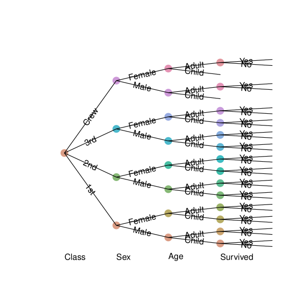
Figure 3: Left: Staged tree m.full where all vertices in the same stratum are in a different stage: there are 29 different stages. Colors in different strata can be equal. Right: Staged tree m.indep where all vertices in the same stratum are in the same stage: there are 4 different stages. The labels at the bottom denote the variable associated to a stratum.

Notice that there are no crew members, either male or female, who are children and this is correctly reflected in the trees in Figure 3 since the subtree associated to such events are collapsed (by default the argument join_unobserved is set to TRUE). The name of these collapsed vertices is set to "na" with the argument name_unobserved.

Using the staged tree m.full or m.indep as starting point, structural learning algorithms can be used to infer the staging structure from the data. The hill-climbing algorithm implemented in stages_hc can receive in input both m.full and m.indep (since it embeds also a splitting stage move). Whilst backward algorithms (implemented in stages_bhc, stages_fbhc and stages_bhcr) and clustering algorithms (implemented in stages_bj, stages_hclust and stages_kmeans) start from the m.full tree. For illustration purposes, the stages_hc function is used with the m.indep tree, whilst stages_bj is used with m.full. R> mod1 <- stages_hc(m.indep) R> mod2 <- stages_bj(m.full, thr = 0.1)

The stages_hc function has BIC as a default score, while the default distance for stages_bj is the symmetrized Kullback-Leibler divergence, with threshold $0.1$ in this example. The learned mod1 and mod2 are plotted in Figure 4. Both staged trees suggest that the variables are dependent in a non-symmetric fashion and thus suggest context-specific independences. The stage structures of the two trees are quite different and may be affected by the choice of threshold in mod2. However, they also share some common features: for instance, both state that the distribution of Male/Female is the same for passengers in the first and second class.

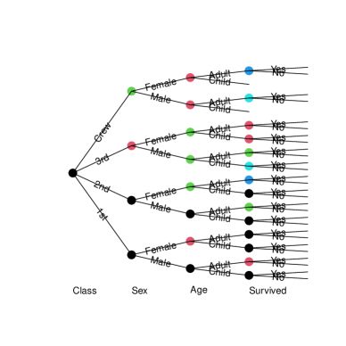
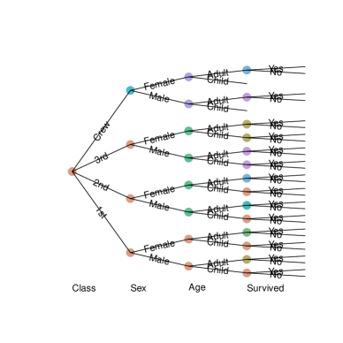
Figure 4: Staged trees mod1 (left) and mod2 (right) learned using the stages_hc and the stages_bj algorithms, respectively.

Since all structural learning algorithms take as input a staged tree, it is possible to refine a learned model: for instance the model mod2 learned using a backward algorithm may be refined using a standard hill climbing algorithm. R> mod3 <- stndnaming(stages_hc(mod2)) R> plot(mod3, ignore = NULL, + cex_label_nodes = 1.5, cex_nodes = 0, font = 2) The resulting staged tree is reported in Figure 5. For illustrative purpose we report there the full tree (by setting ignore = NULL) and the numbering of the stages after renaming them with the function stndnaming. The two staged tree structures in mod1 and mod3 are compared through the compare_stages function, whose output highlights in red the nodes in different stages. Different methods can be used to compare two staged tree structures, here the "stages" method is used: it checks if the same exact stages are present in both models.

R> compare_stages(mod1, mod3, method = "stages", plot = TRUE) [1] FALSE

Figure 5 shows that the two models have the same stage structure over the Sex and Survived variables, but they highly differ over Age.

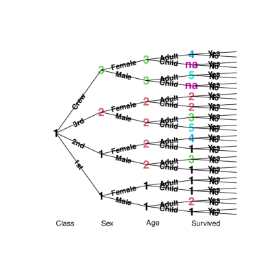
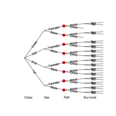
Figure 5: Staged event tree mod3 (left) and output of the compare_stages function between models mod1 and mod3 (right). Vertices depicted by a red dot in the right plot correspond to vertices for which the staging structure differs.

The model selection criteria AIC and BIC can be used to choose the best fitting model. R> cbind(AIC(mod1, mod2, mod3), BIC = BIC(mod1, mod2, mod3)$BIC)\Soutput dfAICBICmod11510364.4910449.94mod21510390.3710475.82mod31510365.0210450.47Accordingtobothcriteria,\code{mod1}isthebestfittingmodelamongthosetried.Itisnotsurprisingthat\code{mod2}obtainstheworstBICscoressinceitwasestimatedwiththe\code{stages_{b}j}functionthatjoinsstagesfollowingadistancebasedheuristicandthusnottheminimizationoftheBICscore.\par\par\par\par$

4.2 Bayesian networks as staged trees

stagedtrees has the capability of translating a BN learned with the bnlearn package into a staged tree. To use bnlearn the dataset Titanic needs to be converted into a data frame.

R> titanic.df <- as.data.frame(Titanic) R> titanic.df <- titanic.df[rep(row.names(titanic.df), titanic.df$Freq),1:4]ThehcfunctionofbnlearncanbeusedtolearnthegraphoftheBNreportedinFigure\text{<a href="\#S4.F6" title="Figure 6 ‣ 4.2 Bayesian networks as staged trees ‣ 4 Usage of the stagedtrees package ‣ The proglangR Package pkgstagedtrees for Structural Learning of Stratified Staged Trees" class="ltx\_ref ltx\_font\_italic"><span class="ltx\_text ltx\_ref\_tag">6</span></a>}left.R>library(bnlearn)R>mod.bn<-bnlearn::hc(titanic.df)R>plot(mod.bn)bn.fitreturnsanobjectofclassbn.fitwhichcanbeturnedintoanobjectofclasssevtusingtheas{}_{s}evtfunction.sevt{}_{f}itisusedtocomputealsothestageprobabilitydistributions.BelowtheRcode.R>mod.bn<-bn.fit(mod.bn,titanic.df)R>bn.tree<-sevt{}_{f}it(as{}_{s}evt(mod.bn),data=titanic.df,lambda=0)R>plot(bn.tree)\text{Figure 6Figure 66Figure 66Left}$