A Machine Learning-based Approach to Build Zero False-Positive IPSs for Industrial IoT and CPS with a Case Study on Power Grids Security

Abstract

Intrusion Prevention Systems (IPS), have long been the first layer of defense against malicious attacks. Most sensitive systems employ instances of them (e.g. Firewalls) to secure the network perimeter and filter out attacks or unwanted traffic. A firewall, similar to classifiers, has a boundary to decide which traffic sample is normal and which one is not. This boundary is defined by configuration and is managed by a set of rules which occasionally might also filter normal traffic by mistake. However, for some applications, any interruption of the normal operation is not tolerable e.g. in power plants, water distribution systems, gas or oil pipelines, etc. In this paper, we design a learning firewall that receives labelled samples and configures itself automatically by writing preventive rules in a conservative way that avoids false alarms. We design a new family of classifiers, called $\mathfrak{z}$-classifiers, that unlike the traditional ones which merely target accuracy, rely on zero false-positive as the metric for decision making. First, we analytically show why naive modification of current classifiers like SVM does not yield acceptable results and then, propose a generic iterative algorithm to accomplish this goal. We use the proposed classifier with CART at its heart to build a firewall for a Power Grid Monitoring System. To further evaluate the algorithm, we additionally test it on KDD CUP’99 dataset. The results confirm the effectiveness of our approach.

I Introduction

Intrusion Prevention Systems (IPS) are security systems that monitor and control the traffic coming in or going out of the network based on a set of pre-defined rules [1]. They usually protect the perimeter of the networks and keep the insiders away from the malicious attacks launched from outside. The most well known examples of IPSs are firewalls.

In delay sensitive applications, where continuity of operation is vital, blocking a legitimate traffic by mistake is not tolerable. This could be disruption in e.g. industrial Cyber Physical Systems (CPS) or governmental services. Some tried solving the issue by mutual authentication of interacting entities [2], however, the majority rely on IPSs. Classic intrusion detection mechanisms rely on classification of samples and divide them into benign and malicious [3, 4, 5]. The border is usually drawn by using a cost minimization algorithm. However, this does not guarantee a zero false alarm and occasionally legitimate traffic is filtered.

Currently, firewalls are mostly configured by experts manually and with the update of attack samples, they are hardly updated, since modifying the rule sets becomes very complex especially when you do not want to tamper with the normal traffic in organizations and industrial applications where business continuity is crucial [6, 7]. Leaving all the decision makings to Intrusion Detection Systems (IDS) is also problematic as IDSs are usually passive systems and have processing limitations which hinder the precise inspection of samples when they are overloaded [8, 9, 10, 11, 12, 13].

In this paper we aim to design a next generation learning firewall that receives labelled samples (e.g. from a supervised Intrusion Detection System (IDS)) and configures itself automatically by writing preventive rule sets in a conservative way that avoids false alarms. In other words, we assume that malicious and normal samples are fed to an automated algorithm of writing preventing rules in the firewall so that it does not block any normal or benign traffic (zero false positive). This is vital in applications where normal operation interruption is not tolerable e.g. in governmental services or cyber-physical systems like power plants, water distribution systems, etc. We design a new family of classifiers that unlike the traditional ones which merely target accuracy, rely on zero-false-positive as the metric for decision making. We try to use iterative methods to accomplish this. The cost paid is an increase in the false negative rate which we tend to minimize.

We leave the grey area to the IDS as it may evolve and improve over the time. However, the learning firewall proactively prevents the damage compared to the passive approach of letting the traffic in and then decide. Besides, it will reduce the load of the IDS too so that it can then increase the complexity or depth of analysis for the remaining traffic. At the final stage, the output of this new classifier is automatically translated into non-conflicting firewall rules. We conduct some experiments on real-world datasets obtained form industrial systems to show how the our approach works.
The rest of this paper is organized as follows: In Section II we review the related work. Section III studies the problem of achieving zero false positive rates and then presents a novel algorithm to make it possible. Section IV tests the algorithm on a power grid monitoring system as well as KDD CUP’99 datasets. Finally, the paper is concluded in Section V.

II Related Work

Several papers focused on increasing the accuracy, speed of traffic recognition or rule enforcement [14, 15, 16, 17]. For example, the aim of [14] is to reduce the memory usage in Internet traffic classification methods using the decision trees. Similarly, in [15, 16, 17], the authors worked on the fusion of rules in Cisco and Palo Alto firewalls.

Some scientists tried to optimize the rules and their sequence of appearance. In firewalls, the rules are executed in order, and the ones appearing first have higher priority. Therefore, if a packet or data sample is to be passed (or be blocked), performance-wise, it is better to put the corresponding rules at the top. In [18, 19], the authors have worked on the optimization of rules and their order of appearance.

Due to the issue of rule preference, sometimes conflicts are found among them. Imagine a rule lets the packet pass while another one shall block it. In this case, the one that appear first in the list determines the result. Many articles have focused on eliminating such inconsistencies among firewall rules [20, 21, 22, 23].

In a related effort, the authors of [24] presented model checking techniques and focused on finding violations of some predefined policies in the rules. They also showed how the developed methods can be used in IPv6 networks.

At a bigger scale, some researchers tried to find ways of investigating whether firewalls of different parts of the same network are following similar policies or not, especially in industrial networks. For example, [25] has provided a semantic basis for expressing and comparing policies applied in every firewall, which in turn can form the basis for a macro judgment of compliance with general (e.g. organizational) policies.

In a valuable effort, the same group [26], in addition to addressing the above problem, proposed the idea of automating firewall configuration for SCADA systems. This idea was developed in the capacity of the ANSI/ISA 62443 standard which is intended to express holistic security policies. The authors tried to add extended features to the ones the standard proposes in order to enable the firewall to use policies for autoconfiguration. Although this research took a step towards autoconfiguration, it was not designed to use the learned attack patterns and merely limited a industrial network interconnections and partitioned it into zones according to the policies.

In [27], the researchers similarly worked on automating firewall rule configuration based on a set of given policies. In this study, Mignis tool was used for generating the rules based on the descriptive semantics derived from policies. The goal was to implement high level policies and not to learn attacks for prevention purposes or to lower false positives.

In [28, 29, 30], the authors have addressed the problem of learning firewall rules, but not by the network owner. They investigate it from an outsider’s perspective who intends to discover the rules written in the firewall by trial and error e.g. through sending requests and interpreting the responses.

In [31], a firewall is designed based on a set of fuzzy rules. In this method, the membership level of the input packet to a set of predefined fuzzy functions is evaluated, and then the final decision (either rejection or acceptance) is made based on the aggregated information. The approach taken in this study is more like a fuzzy IDS whose decisions are enforced by an actuating IPS e.g. a firewall. However, in this paper, the problem of false decisions has not yet been addressed.

A similar research has been done in the context of http and web applications, but with learning capabilities [32]. It is assumed that the normal behavior is fed into the system in the form of XML, and any behavior that is classified as abnormal is filtered. However, due to the lack of attention to false positives and false negatives, the performance of this method is questionable in industrial applications.

In [33], in addition to working on speed enhancements, moved towards the learning capability in firewalls. They used a Huffman tree of rules for this purpose. Learning happens by adaptations and changes in this tree. However, the learning criterion is merely met by crossing some hard thresholds over the measured indicators.

A network IDS based on the biological immune mechanism has been proposed in [9]. It aims lowering false positives. In this method, three monitor agents (located in different parts of the network) provide co-stimulation signals to the intrusion detectors in order to reduce false positive alarms. Similarly, the authors in [8] used a hybrid neuro-fuzzy approach to reduce the number of false alarms in IDSs. The proposed approach was experimented with different background knowledge sets in DARPA 1999 dataset. The authors concluded through simulations that their approach required less background knowledge sets compared to other approaches. In a relevant try, [10] used neural network to build an IDS that considers the cost ratio of false negative errors to false positive errors. The authors stated that compared with false positive errors, false negative errors incur a greater loss thus must be lowered.

As explained, little work has been done in the area of automating the connection of firewalls to the units such as IDSs and attack intelligence systems for enhancing the prevention task. When we add the zero false positive requirement to the problem, there remains no background in the literature.

III The Proposed Approach: Zero-False Positive Automatic Firewall Rule Generation

In this section, we first look into extending traditional classifiers like SVM to achieve a zero false positive rate. By giving a set of examples, we show why this approach cannot serve the purpose well. Then, a novel iterative algorithm is presented which yields zero positive results and can accommodate almost any classifier at its core. At the end of this section, we discuss how a tree-based classifier can turn the algorithm output into non-conflicting firewall rules.

III-A Problem Description and Articulation

Without loss of generality, we focus on the binary classification problem. We start with the linear case. Nonlinearity can be added by e.g. using kernels later though the algorithm we propose is generic and can support almost every classifier.

We assume the two classes are nonseparable. We do not have any problem with separable cases since they lead to zero false positive results. We do not elaborate which classifier is capable of doing so at this stage. However, for the case of linearly separable classes, there exists a line that correctly separates the samples with zero error as in e.g. SVM [34].

To describe the research problem, we use the linear case. However, this will be relaxed later. Fig. 1a shows a two-class set of data samples which are linearly non-separable. A linear boundary has been drawn just as an example to serve the development of subsequent formula. Let us denote the labelled (training) samples of Class 1 (+) and Class 2 (-) by $\boldsymbol{x}_{i}~{};~{}i=1,...,N$. The goal is to find a boundary that achieves zero false positive; the statement that once decided that an input sample is +, is not wrong.

This means that no sample of Class 2 shall be classified as 1 (or +). You may imagine Class 1 is the set of attack samples and Class 2 is the set of normal ones in an industrial network security context. Therefore, no normal sample should be classified as malicious as it will be blocked and this interrupts the normal system operation.

Similarly, we could consider biometric security systems. In physical security systems, like fingerprint readers, false positives (false acceptances) are not tolerable, though they come at the cost of some extra false negatives. It is preferred that the granted permissions are always correct, even if sometimes legitimate users have to re-enter their fingerprints for the reader to pick. However, in insensitive commercial applications, manufacturers tend to compromise some security for functionality as repetitive data entry is not convenient.

One can achieve a zero false positive rate, but it might come at the cost of a low true negative rate (or high false negative rate). We tend to additionally minimize false negatives, or equivalently, maximize true negatives. This could be translated into minimizing the number of samples in Class 1 ($+$) that fall on the other side of the boundary and are classified as ($-$). The two above-mentioned goals are not easy to achieve simultaneously. In the next subsection, we mathematically show how a classic classifier works and then in Subsection C, extend it in a try to make a zero false positive classifier.

III-B Formulation of the Classic Approach (SVM)

There are different methods for formulation of linear classifiers facing mixed data. Normally, at some point during the development, one faces a discrete variable counting the number of misclassified samples which is usually replaced by a not-so accurate continuous approximation to keep the problem convex [34].

(a)

(b)

Figure 1: (a) Traditional classification of linearly non-separable classes in a trade of between gutter and the weight of misclassified samples. The circles show correctly classified samples and the square ones are misclassified. (b) Zero false-positive classification using the same classic principles but with different criteria.

We formulate the binary classification problem following the classic approach for SVM as an example. However, later during the process, we diverge from the normal definitions as we are following different targets. In SVM, depending on where the training sample $\boldsymbol{x}_{i}$ lies with respect to the linear boundary $\boldsymbol{a}.\boldsymbol{x}_{i}+b_{0}=0$, we will have different conditions. If $y_{i}$ is a scalar variable whose value is +1 for the $\boldsymbol{+}$ samples and -1 for the $\boldsymbol{-}$ ones, we can express these conditions with respect to the boundary as below:

• The sample is correctly classified and falls outside the gutter (band) specified by $\boldsymbol{a}.\boldsymbol{x}_{i}+b_{0}=\pm 1$. For such samples which are shown by circles around them and lie outside the gutter in Fig.1a, we have:

  $$y_{i}(\boldsymbol{a}.\boldsymbol{x}_{i}+b_{0})\geq 1$$ (1)

  where equality happens when the sample (support vector) is on either of the two parallel gutter lines.

• The sample is correctly classified with the given $\boldsymbol{a}$ and $b_{0}$, but lies inside the gutter:

  $$0\leq y_{i}(\boldsymbol{a}.\boldsymbol{x}_{i}+b_{0})<1$$ (2)

  Again, since these are classified correctly, they are shown by circles in Fig. 1(a).

• The sample is classified in the wrong class:

  $$y_{i}(\boldsymbol{a}.\boldsymbol{x}_{i}+b_{0})<0$$ (3)

  These samples are shown by squares in Fig. 1(a).

Some rewrite all the three in a single equation by using a slack variable as:

$$y_{i}(\boldsymbol{a}.\boldsymbol{x}_{i}+b_{0})\geq 1-\eta_{i}$$ (4)

where $\eta_{i}=0$ in the first case, $0<\eta_{i}\leq 1$ in the second, and $\eta_{i}>1$ in the third. Usually, the classification goal is to make the gutter as wide as possible while keeping the number of misclassified samples minimal. With the above formulation, the gutter width will be $2/||\boldsymbol{a}||$ [34]. For mathematical convenience, it is usual to minimize $\frac{1}{2}||\boldsymbol{a}||^{2}$ instead. The cost function for such a minimization problem would be:

$$J(\boldsymbol{a},b_{0},\boldsymbol{\eta}) =\frac{1}{2}||\boldsymbol{a}||^{2}+c\sum_{i=1}^{N}\mathcal{F}({\eta_{i}})$$ (5)

$$\mathcal{F}(\eta_{i}) =\begin{cases}1,&\text{if}\ \eta_{i}>0\\ 0,&\text{if}\ \eta_{i}=0\end{cases}$$ (6)

To remove the discontinuous functions and make the problem convex [34], the the term $\sum_{i=1}^{N}\mathcal{F}({\eta_{i}})$ is usually approximated by $\sum_{i=1}^{N}{\eta_{i}}$, which does not actually minimize the number of misclassified samples, but rather a cost function related to that:

$$\underset{\boldsymbol{a},b_{0}}{\arg\min}~{}J(\boldsymbol{a},b_{0},\boldsymbol{\eta}) =\frac{1}{2}||\boldsymbol{a}||^{2}+c\sum_{i=1}^{N}{\eta_{i}}$$ (7)

$$sbj.~{}to:~{}~{} y_{i}(\boldsymbol{a}.\boldsymbol{x}_{i}+b_{0})\geq 1-\eta_{i}$$

$$\eta_{i}\geq 0$$

where the positive constant $c$ specifies the importance of the second term compared to the gutter width. This was a short introduction to the classic problem formulation.

III-C Extension of the Classic Approach ($\mathfrak{z}$-SVM)

The above formulation does not guarantee a zero false positive rate. Fig. 1a shows a linearly non-separable constellation in which one sample from each class has been misclassified. Obviously, in Eq. (8), the optimization algorithm does not have any preference over the classes. We can extend the classic formulation towards giving preference to one class and outputting zero false-positive results. If we break down the number of training samples as $N=n_{n}+n_{p}$, we can write:

$$\underset{\boldsymbol{a},b_{0}}{\arg\min}~{}J(\boldsymbol{a},b_{0},\boldsymbol{\eta}) =\frac{1}{2}||\boldsymbol{a}||^{2}+c_{1}\sum_{i=1}^{n_{n}}{\eta_{i}+c_{2}\sum_{i=n_{n}+1}^{N}{\eta_{i}}}$$ (8)

$$sbj.~{}to:~{}~{} y_{i}(\boldsymbol{a}.\boldsymbol{x}_{i}+b_{0})\geq 1-\eta_{i}$$

$$\eta_{i}\geq 0$$

where $c_{1}>c_{2}$. We refer to this classifier as $\mathfrak{z}$-SVM. The goal is to achieve something like Fig. 1b with zero false positives while keeping the false negatives as low as possible.

III-D The Issues with $\mathfrak{z}$-SVM

In the previous subsection, we developed a convex formulation based on the classic approach to increase the cost of misclassification for $-$ samples. By choosing $c_{1}\gg c_{2}$, one can make the optimization algorithm try to zero the number of misclassifications for the negative samples. However, there are a number of issues with this naive approach which can make it impractical in certain scenarios.

III-D1 Continuous Error Approximation

The optimization algorithm is blind to the details of the problem. In certain cases, it deceives us by manipulating the gutter width. Based on Eq. (8), the classification error contributing to the cost function is the sum of $\eta_{i}$ ; $i=1,...,N$. When we want to increase $c$ (e.g. $c_{1}$, hoping to achieve zero false positive), the optimizer tends to make the gutter width smaller to virtually reduce the errors (see Eq. (8)). This is due to the fact that $\eta_{i}$ is a function of the gutter width itself. Fig. 2a to 2c demonstrate this fact.

III-D2 Weight Coefficients Effect

$\mathfrak{z}$-SVM is highly sensitive to $c_{1}$ and $c_{2}$ values. It is not just their ratio that matters, their absolute values are also important along with the $||\boldsymbol{a}||$.

There are three cost components in Eq. (8). If we choose a big value for $c_{1}$ and a rather small one for $c_{2}$, we might achieve a zero false positive rate. However, there is still a probability that this does not happen. For example, if exists a ”$-$” sample deep inside the positive class region, it will contribute a large $\eta_{i}$ whose cost is further boosted by $c_{1}$. However, to make the false positive zero, the algorithm shall move the boundary line and misclassify some positive samples. Each of these samples (let us say $j$) adds $c_{2}\eta_{j}$ to the cost. If the number of such samples is high, their cumulative cost might surpass $c_{1}\eta_{i}$. Therefore, the minimization algorithm might not output a zero false-positive result. This is highly dependent on the constellation of samples, how the classes are mixed, and the choice of $c_{1}$ and $c_{2}$. Fig. 2d demonstrates this issue.

(a)

(b)

(c)

(d)

(e)

(f)

(g)

(h)

(i)

Figure 2: The effect of cost coefficient ($c$) on $\mathfrak{z}$-SVM result: (a) $c_{1}=1$, $c_{2}=1$ (b) $c_{1}=5$, $c_{2}=5$ (c) $c_{1}=50$, $c_{2}=50$ (d) $c_{1}=500$, $c_{2}=50$ (e) $c_{1}=785$, $c_{2}=50$ (f) $c_{1}=800$, $c_{2}=50$ (g) $c_{1}=1000$, $c_{2}=50$. (h) $c_{1}=80$, $c_{2}=5.$

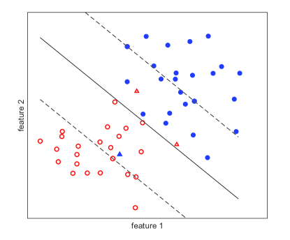
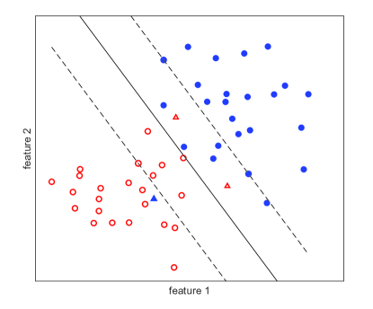
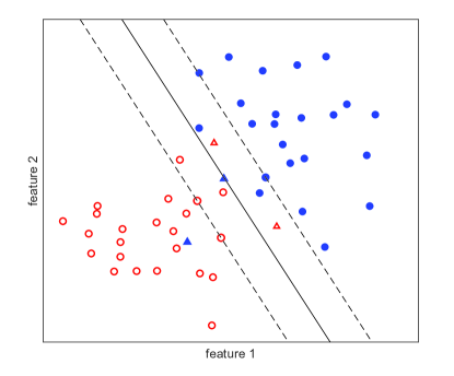
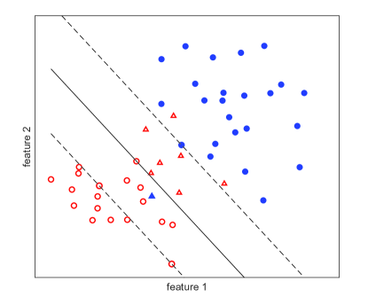
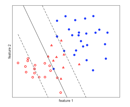
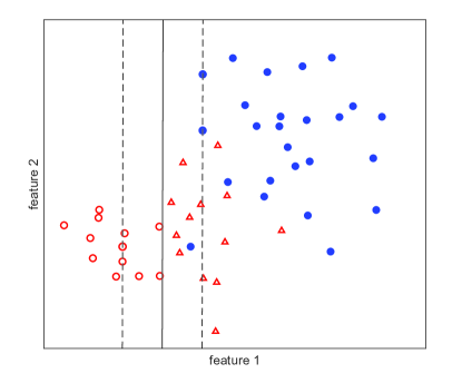
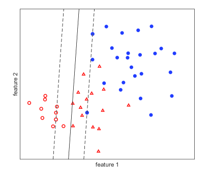
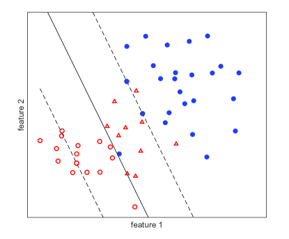
A very large value for $c_{1}$ can solve this issue, but it induces another problem. By choosing such a value for $c_{1}$, the dominant component in the cost function will be the second term. This implies that the gutter width and the $+$ samples misclassification error will have little or no effect. This might for example lead to a boundary that misclassifies too many positive sample in order to keep $c_{1}\sum_{i=1}^{n_{n}}\eta_{i}$ minimum. Fig. 2e to 2g show this phenomenon. Comparison of Fig. 2f and Fig. 2h which have the same $c_{1}/c_{2}$ ratio shows that the third cost component, i.e. $||\boldsymbol{a}||$ can significantly change the final result. Note that in the settings achieving zero false positive rates, the number of misclassified positive samples are significantly different, ranging from 9 to 16, with Fig. 2e having the minimum number of such samples. The cost coefficients in Fig. 2e are trivially different from those in Fig. 2f, yet the results are very different. This shows how sensitive the final result is to the choice of $c_{1}$ and $c_{2}$.

Figure 3: Flowchart of the proposed iterative classification algorithm ($\mathfrak{z}$-Classifier). The goal is to achieve zero false positive rate.

III-D3 Sample Unbalance Problem

The training sample unbalance problem is very well known. This is not something specific to $\mathfrak{z}$-SVM. Imagine that there are merely a few negative training samples and too many positive ones. In such occasions, the cost of misclassification for the negative samples is practically capped and the optimizer might decide to minimize the cost function based on the dominant factor defined by the too-many positive samples. This implies that we need to adjust $c_{1}/c_{2}$ per case.

The above discussions showed some of the problems of $\mathfrak{z}$-SVM; an example of traditional classifiers extension. Many of these problems pertain to the fact that the counting function (e.g. of Eq. (6)) is replaced with an approximate alternative in the convex problem development process. One can of course stick with original optimization problems (e.g. Eq. (5)) and try to extend them for zero false positive goal while honoring the discrete constraints (like Eq. (6)). However, the result will be a non-convex or discrete problem at the end.

In the next section, we propose a novel algorithm for this purpose. We use classic approaches at the core of the algorithm but iteratively prune the samples based on its outputs to achieve zero false positive rates with minimum number of false negatives. Minimizing the number of false negatives will allow the firewall to capture as many malicious samples as possible and lower the load of the sophisticated IDS, if ever installed. Finally, using a tree classifier at the core, we test our algorithm and show how its output can be translated into simple non-conflicting firewall rules.

Given a classifier, false positives can be avoided if one sacrifices some of the positive samples. We suggest that this is done by removal. It can be proven that a removing strategy always converges to a zero-false positive result. However, the question is which positive samples shall be sacrificed to make this happen. We can represent the problem as a binary satisfiability one. Imagine the positive samples are the set of variables, each being represented by a bit. A value of 0 for a bit implies that the corresponding sample shall be removed from the set. Regarding the example of Fig. 1, this binary coding will be like $\{b_{A},b_{B},b_{C},b_{D},b_{E},...\};b_{i}\in\{0,1\}$. Now, given the classifier $\mathcal{C}$, the remaining set can be tested to see if its samples satisfy separability. Therefore, the problem is analogous to a boolean satisfiability (SAT) problem. It can be proven that the problem is always satisfiable. In general, finding an assignment of zeros and ones that has the minimum number of variables set to one (or similarly to zero) is NP-complete, even for a satisfiable 2-SAT problem [35]. This is sometimes called Min Ones $k$-SAT problem in the literature. The solution is not always unique though. For example, in Fig. 1 and with a linear $\mathcal{C}$, both $\{0,0,1,1,1,1,...\}$ and $\{0,1,1,0,1,1,...\}$ will satisfy the separability thus the resultant boundaries can be acceptable. Although there could be several answers, some additional constraints in the cost function (like maximum gutter width or distance to the border) can reduce the set of answers.

III-E The Proposed Zero-FP Classifier ($\mathfrak{z}$-Classifier)

The proposed algorithm is an iterative classification method which achieves a zero false detection rate for the positive class. It is a swarm algorithm whose particles are reduced datasets. Each reduced dataset consists of all the negative samples and some of the positive ones. In this sense, we can represent each particle with a binary coding similar to before i.e. $\{b_{1},b_{2},...,b_{n_{p}}\};b_{i}\in\{0,1\}$, where for the sake of simplicity, we have removed the 1s of the negative class members as they are always present. Each particle follows an algorithm which is illustrated in Fig. 3. The grey box is where it uses the knowledge obtained by other particles.

Each particle starts with an initial dataset which is derived from the original one by removing some of the positive samples in order to become separable. Ideally, this initial dataset has only one positive sample, and all the negative ones. Given the classifier $\mathcal{C}$, one can do an initial classification on the original dataset and use the true positives as candidates to make this initial dataset. Every particle’s reduced dataset goes through a classification by using $\mathcal{C}$. In each iteration, if the result shows separability of the set (zero false positive and zero false negative), the set is compared against the best result obtained by other particles so far. The comparison criterion could be a predefined fitness function e.g. the number of positive samples included as we intend to minimize the number of false negatives. If the particle’ reduced set yields a better score, the best record is replaced with its set. Then, the boundary model obtained through the process is applied to the original dataset (as a test set) and the new true positives are tentatively added to the particle’s set for the next iteration. This is done by setting their flag to 1. Moreover, some extra positive samples that are misclassified by this boundary are also selected and added to the set. There can be different selection criteria for this purpose, however, we suggest that one uses the global best (as in Particle Swarm Optimization) for this purpose. For example, one can use weighted random selection to pick $k$ samples from the set of falsely classified positive samples (of the original set) and add them to the particle’s set. Obviously, the positive samples included in the best set should have more weight in this selection.

On the other hand, throughout the iterations, if a particle’s set becomes inseparable at some point, it will undergo a pruning operation. The pruning is initially done by removing the positive samples that have created false negatives. If this does not help (which will be known in the next iteration(s)) or the source of inseparability is non-zero false positive, the weight of the negative samples contributing to the false positives is increased. This can be done by e.g. duplicating those negative samples in the particle’s dataset. As it can be seen, the reduced dataset of particle is not necessarily a subset of the original dataset yet they are related. The pruning continues over iterations until the set becomes separable again. The whole addition/removal process terminates when either the target false negative is met or the maximum number of allowed iterations is reached. Algorithm 1 shows $\mathfrak{z}$-Classifier.

Algorithm 1 The Proposed Iterative Classification Technique with Zero False Positive ($\mathfrak{z}$-Classifier)

1:Training Set($\mathcal{T}$), Performance Target/Stop Criterion

2: Zero False Positive Classification

3:Create initial separable particle sets $S_{1},...S_{k}$

4:Determine the $Best$ set (with the most positive samples)

5:while Stop Criterion/Performance Target is not met do

6:   for each $S_{i}$ do

7:      Classify $S_{i}$ with $\mathcal{C}$ and find the boundary $\mathcal{B}_{i}$

8:      if $S_{i}$ is separable then

9:         Update the $Best$ if $S_{i}$ is more fit

10:         Apply $\mathcal{B}_{i}$ to $\mathcal{T}$ & add the true positives to $S_{i}$

11:         Use the $Best$ and $S_{i}$ knowledge to add $k_{i}$ false positive samples to $S_{i}$

12:      else

13:         if there is false negatives then

14:            Remove false negative samples from $S_{i}$

15:         else

16:            Duplicate false positive samples in $S_{i}$

17:         end if

18:      end if

19:   end for

20:end while

IV Evaluation Results and Discussions

Here, we evaluate $\mathfrak{z}$-Classifier by testing it on two datasets. We take the CART algorithm as our classifier. Classic firewalls can define rules by combining clauses that put constraints on the values of features. However, each clause merely constrains one feature. For such construction, tree-based classifiers like CART produce more compatible results. In the simulations, the population size was 5 and $k_{i}$ was increased exponentially by a factor of 1.5 (from 1) for faster convergence. It was reset to 1 every time the set became non-separable.

IV-A Power System (Smart Grid) Dataset

Smart grids or power systems have supervisory control systems interacting with different smart electronic devices. They are complemented by network monitoring devices such as SNORT and Syslog. Some researchers created a dataset of attacks launched in power systems [36, 37]. In their scenario, it is assumed that an actor gains access to a substation network and poses an insider threat by issuing commands from the substation switch. The scenarios studied were (1) Short-circuit fault, (2) Line maintenance (3) Remote tripping command injection (Attack), (4) Relay setting change (Attack), and (5) Data Injection (Attack) [36, 37]. This study worked on events categorized in binary classes which contained 37 event scenarios grouped as either attack (28 events) or normal operations (9 events). We used a subset of the dataset with 1861 normal and 3415 attack samples described by 128 features. Date and time were taken out of the dataset records as we did not want the classifier to rely on those for detection. The results of applying $\mathfrak{z}$-Classifier on this dataset are shown in Table I. As one can see and similar to before, the proposed classifier always maintains a zero false positive output.

TABLE I: $\mathfrak{z}$-Classifier performance on the power grid dataset of [36, 37]

Iterations	TN	TP	FN	FP
10	1861	320	3095	0
50	1861	888	2527	0
100	1861	2211	1204	0
500	1861	3231	184	0
1000	1861	3353	62	0

IV-B Results of KDD CUP’99 Dataset

KDD Cup’99 dataset has been developed by MIT Lincoln Laboratory in 1999 [38]. We use a subset of the dataset that has 10% of the total records (494,021). Every record has 41 features and contains a label for the sample class. Along with normal samples, there are 24 types of attacks in the training set which fall into four categories. However, we turned all the attack labels into malicious so that the algorithm is left with a decision of ACCEPT or REJECT for each sample. Even a simple classifier obtained after 10 iterations can capture 138,869 out of 204,458 malicious samples with zero false positive. The complete tree after 1000 iterations yields much better results which are reported in Table II. Please note that just like any learning classifier, $\mathfrak{z}$-Classifier is also prune to over-fitting. We noticed over-fittings after the 100th iteration with KDD CUP’99 dataset. One can adopt traditional best practices to avoid this phenomenon.

TABLE II: $\mathfrak{z}$-Classifier performance on KDD CUP’99 dataset.

Iterations	TN	TP	FN	FP
10	289,542	138,869	65,589	0
50	289,542	204,167	291	0
100	289,542	204,425	33	0
500	289,542	204,432	26	0
1000	289,542	204,432	26	0

Translation of the $\mathfrak{z}$-Classifier output to firewall rules is a trivial task now. For the tree described before, the first few rules of a default-allow firewall will be like:

IF $x_{29}<0.255$ & $x_{35}\geq 0.145$ & $x_{32}<97.5$ then REJECT IF $x_{29}\geq 0.255$ & $x_{37}\geq 0.055$ & $x_{23}\geq 4.50$ then REJECT

$\vdots$

in which $x_{29}$ (’same_srv_rate’) shows the percentage of connections to the same service, $x_{35}$ (’dst_host_diff_srv_rate’) is the percentage of connections to different services, $x_{32}$ (’dst_host_count’) is the number of connections to the same destination host, $x_{37}$ (’dst_host_srv_diff_host_rate’) shows the percentage of connections to the same service coming from different hosts, and $x_{23}$ is the number of connections to the same host as current connection in the past two seconds.

V Conclusion

Rejecting legitimate traffic by mistake is not tolerable in real-time industrial systems e.g. power systems. Intrusion detection systems, if ever installed, also have limited capacity of inspection and it is preferred that the attacks are filtered at intrusion preventions systems such as firewalls as much as possible. In this study, a new classifier is introduced that can help in building self-organizing learning firewalls. Current classifiers tend to minimize a generic cost function which does not necessarily yield zero false positive results. In this paper, we proposed an algorithm that can turn any generic classifier into a zero false positive one. One can use this classifier to build a self-organizing and learning firewalls. In the design of this new approach zero false positive (or negative) rate has been set as the goal, while the false negative (or positive) rate is kept minimum. The designed classifier was tested on two datasets; a power grid dataset and KDD CUP’99 dataset. We also showed how a tree-based classifier can help us automate writing zero-false positive firewall rules.

Appendix A Satisfiability with the Removal Strategy

Theorem 1. Given a dataset with two classes and a sound classifier like $\mathcal{C}$, an iterative removal strategy that takes the false positive samples out in each iteration will always lead to a zero false positive result.

Proof. Assume that the training dataset is $(x_{i},y_{i})$ where $i=1,2,...,m$ and $y_{i}\in\left\{1,-1\right\}$. The zero FP algorithm applies a sound classifier $\mathcal{C}$ as a core classifier which minimizes a predefined cost function like $J$.

First, the algorithm starts on the complete and original dataset. After classification, there are two types of misclassified samples which make the classification errors. The first one corresponds to false negatives $(E^{P\rightarrow N})$, and the second one is related to false positives $(E^{P\rightarrow N})$. The cost function of the classifier is $J(E_{0}^{P\rightarrow N},E_{0}^{N\rightarrow P})$, where the 0 superscript shows the iteration number. According to the zero FP algorithm, the positive samples which make $E^{P\rightarrow N}$ must be removed from the original data set at this stage. After applying the classifier boundary to the new data set (after removal), $E^{P\rightarrow N}$ will be zeroed. Hence, the cost function of the zero FP algorithm at this stage becomes $J(E_{1}^{N\rightarrow P})<J(E_{0}^{P\rightarrow N},E_{0}^{N\rightarrow P})$. This inequality can be rewritten as:

$$J(E_{1}^{N\rightarrow P})=r_{1}~{}J(E_{0}^{P\rightarrow N},E_{0}^{N\rightarrow P})$$ (9)

where $0\leq r_{1}\leq 1$. Sequentially, the sound classifier provides a new classification boundary for the modified dataset whose cost function is $J(E_{2}^{P\rightarrow N}$, $E_{2}^{N\rightarrow P})$. Since the dataset is modified, $\mathcal{C}$ tried to minimize the misclassification errors so that it is less than (or in the worst case equal to) the previous iteration, i.e. $J(E_{2}^{P\rightarrow N}$ , $E_{2}^{N\rightarrow P})<J(E_{1}^{N\rightarrow P})$. Hence,

$$J(E_{2}^{P\rightarrow N},E_{2}^{N\rightarrow P})=q_{1}~{}J(E_{1}^{N\rightarrow P})$$ (10)

where $0\leq q_{1}\leq 1$. Similarly the algorithm removes the positive samples which have been misclassified. At the $k^{th}$ iteration, the cost function will be:

$$J(E_{k}^{P\rightarrow N},E_{k}^{N\rightarrow P})=q_{k}~{}J(E_{k-1}^{N\rightarrow P});~{}~{}~{}0\leq q_{k}\leq 1$$ (11)

and at the $k+1^{th}$ one,

$$J(E_{k+1}^{N\rightarrow P})=r_{k}~{}J(E_{k}^{P\rightarrow N},E_{k}^{N\rightarrow P});~{}~{}~{}0\leq r_{k}\leq 1$$ (12)

This way, at each iteration a reduced set is prepared for the next iteration. By substituting Eq. (11) in Eq. (12),

$$J(E_{k+1}^{N\rightarrow P})=(r_{k}~{}q_{k})~{}J(E_{k-1}^{N\rightarrow P})$$ (13)

Similarly,

$$J(E_{k+1}^{N\rightarrow P})=\left(\Pi_{k=1}^{N}(r_{k}~{}q_{k})\right)~{}J(E_{0}^{P\rightarrow N},E_{0}^{N\rightarrow P})$$ (14)

As $\Pi_{k=1}^{N}(r_{k}~{}q_{k})$ goes to zero, we have

$$\lim_{k\rightarrow\infty}J(E_{k+1}^{N\rightarrow P})=0$$ (15)

Notice that $\text{max}(N)$ is the number of positive samples. Therefore, the cost function of the zero FP algorithm with a sound cost-minimizing classifier will converge to zero, and all negative samples will be truly classified.

References

- [1] X. Zhang, C. Li, and W. Zheng, “Intrusion prevention system design,” in Int. Conf. on Computer and Information Technology, 2004, pp. 386–390.
- [2] A. Mohammadi-nodooshan, Y. Darmani, R. Jalili, and M. Nourani, “A robust and efficient sip authentication scheme,” Elsevier Scientia Iranica Transactions in Computer Science and Electrical Engineering, 2010.
- [3] H.-J. Liao, C.-H. R. Lin, Y.-C. Lin, and K.-Y. Tung, “Intrusion detection system: A comprehensive review,” Journal of Network and Computer Applications, vol. 36, no. 1, pp. 16–24, 2013.
- [4] F. Farivar, M. Sayad Haghighi, S. Barchinezhad, and A. Jolfaei, “Detection and compensation of covert service-degrading intrusions in cyber physical systems through intelligent adaptive control,” in IEEE Int. Conf. on Industrial Technology, 2019.
- [5] F. Farivar, M. S. Haghighi, A. Jolfaei, and M. Alazab, “Artificial intelligence for detection, estimation, and compensation of malicious attacks in nonlinear cyber physical systems and industrial iot,” IEEE transactions on industrial informatics, 2019.
- [6] N. Toorchi, M. A. Attari, M. S. Haghighi, and Y. Xiang, “A markov model of safety message broadcasting for vehicular networks,” in IEEE Wireless Communications and Networking Conference, 2013, pp. 1657–1662.
- [7] A. Arabsorkhi, M. S. Haghighi, and R. Ghorbanloo, “A conceptual trust model for the internet of things interactions,” in 8th International Symposium on Telecommunications, 2016, pp. 89–93.
- [8] R. Alshammari, S. Sonamthiang, M. Teimouri, and D. Riordan, “Using neuro-fuzzy approach to reduce false positive alerts,” in Conf. on Communication Networks and Services Research, 2007, pp. 345–349.
- [9] Y. Qiao and X. Weixin, “A network ids with low false positive rate,” in Cong. on Evolutionary Computation, vol. 2. IEEE, 2002, pp. 1121–1126.
- [10] D. Joo, T. Hong, and I. Han, “The neural network models for ids based on the asymmetric costs of false negative errors and false positive errors,” Expert Systems with Applications, vol. 25, no. 1, pp. 69–75, 2003.
- [11] M. S. Haghighi and K. Mohamedpour, “Neighbor discovery: Security challenges in wireless ad hoc and sensor networks,” in Trends in Telecom. Tech. Intech, 2010.
- [12] S. Barchinezhad and M. S. Haghighi, “Compensation of linear attacks to cyber physical systems through arx system identification,” in 10th Information and Knowledge Technology Conference (ICIKT2019), 2019.
- [13] M. S. Haghighi, F. Farivar, A. Jolfaei, and M. H. Tadayon, “Intelligent robust control for cyber-physical systems of rotary gantry type under denial of service attack,” The Journal of Supercomputing, pp. 1–23, 2019.
- [14] Y.-C. Cheng and P.-C. Wang, “Packet classification using dynamically generated decision trees,” IEEE Trans. on Comp., vol. 64, no. 2, pp. 582–586, 2015.
- [15] C. Diekmann, J. Michaelis, M. Haslbeck, and G. Carle, “Verified iptables firewall analysis,” in IFIP Networking Conf., 2016, pp. 252–260.
- [16] P. Kadam and V. Bhusari, “Review on redundancy removal of rules for optimizing firewall,” Int. Jour. of Research in Engineering and Technology, 2014.
- [17] L. Zhang and M. Huang, “A firewall rules optimized model based on service-grouping,” in Web Information System and Application Conf., 2015, pp. 142–146.
- [18] Z. Trabelsi, L. Zhang, and S. Zeidan, “Dynamic rule and rule-field optimisation for improving firewall performance and security,” IET Inf. Sec., vol. 8, no. 4, pp. 250–257, 2014.
- [19] Y. Zhu, “Optimization design and implementation of gateway based on firewall for access control,” in Int. Conf. on Inf. Science and Tech., 2016, pp. 100–104.
- [20] E. S. Al-Shaer and H. H. Hamed, “Discovery of policy anomalies in distributed firewalls,” in IEEE Conf. of Comp. and Comm. Societies, 2004, pp. 2605–2616.
- [21] S. Khummanee, A. Khumseela, and S. Puangpronpitag, “Towards a new design of firewall: Anomaly elimination and fast verifying of firewall rules,” in Conf. on Computer Science and Software Engineering, 2013, pp. 93–98.
- [22] F. A. Maldonado-Lopez, E. Calle, and Y. Donoso, “Detection and prevention of firewall-rule conflicts on software-defined networking,” in Int. Workshop on Reliable Networks Design and Modeling, 2015, pp. 259–265.
- [23] A. Bouhoula and A. Yazidi, “A security policy query engine for fully automated resolution of anomalies in firewall configurations,” in IEEE Symp. on Network Computing and Applications, 2016, pp. 76–80.
- [24] C. Lorenz and B. Schnor, “Policy anomaly detection for distributed ipv6 firewalls,” in Int. Conf. on e-Business and Telecommunications, vol. 4, 2015, pp. 210–219.
- [25] D. Ranathunga, M. Roughan, P. Kernick, and N. Falkner, “Malachite: Firewall policy comparison,” in IEEE Symp. on Computers and Communication, 2016, pp. 310–317.
- [26] D. Ranathunga, M. Roughan, H. Nguyen, P. Kernick, and N. Falkner, “Case studies of scada firewall configurations and the implications for best practices,” IEEE Tran. on Net. and Serv. Manag., vol. 13, no. 4, pp. 871–884, 2016.
- [27] P. Adao, R. Focardi, J. D. Guttman, and F. L. Luccio, “Localizing firewall security policies,” in IEEE Computer Security Foundations Symp., 2016, pp. 194–209.
- [28] M. Q. Ali, E. Al-Shaer, and T. Samak, “Firewall policy reconnaissance: Techniques and analysis,” IEEE Trans. on Information Forensics and Security, vol. 9, no. 2, pp. 296–308, 2014.
- [29] A. X. Liu, A. R. Khakpour, J. W. Hulst, Z. Ge, D. Pei, and J. Wang, “Firewall fingerprinting and denial of firewalling attacks,” IEEE Trans. on Information Forensics and Security, vol. 12, no. 7, pp. 1699–1712, 2017.
- [30] F. Chen, A. X. Liu, J. Hwang, and T. Xie, “First step towards automatic correction of firewall policy faults,” ACM Trans. on Autonomous and Adaptive Systems, vol. 7, no. 2, p. 27, 2012.
- [31] S.-U. Lar, X. Liao, A. ur Rehman, and M. Qinglu, “Proactive security mechanism and design for firewall,” Journal of Inf. Sec., vol. 2, no. 03, p. 122, 2011.
- [32] C. Torrano-Gimenez, A. Perez-Villegas, and G. Alvarez, “A self-learning anomaly-based web application firewall,” Computational Intelligence in Security for Information Systems, pp. 85–92, 2009.
- [33] A. S. Sairam, R. Kumar, and P. Biswas, “Implementation of an adaptive traffic-aware firewall,” in Int. Conf. on Security of Information and Networks, 2014, p. 385.
- [34] S. Theodoridis and K. Koutroumbas, Pattern Recognition (4th ed.). Academic Press, 2009.
- [35] N. Misra, N. Narayanaswamy, V. Raman, and B. S. Shankar, “Solving min ones 2-sat as fast as vertex cover,” Theoretical Comp. Sci., vol. 506, pp. 115–121, 2013.
- [36] S. Pan, T. Morris, and U. Adhikari, “Developing a hybrid intrusion detection system using data mining for power systems,” IEEE Trans. on Smart Grid, vol. 6, no. 6, pp. 3104–3113, 2015.
- [37] R. C. B. Hink, J. M. Beaver, M. A. Buckner, T. Morris, U. Adhikari, and S. Pan, “Machine learning for power system disturbance and cyber-attack discrimination,” in Int. Symp. on resilient control systems, 2014, pp. 1–8.
- [38] KDD Cup 1999. [Online]. Available: http://kdd.ics.uci.edu/databases/kddcup99/kddcup99.html