Anomalous diffusion in Davydov quantum molecular chain model

Abstract

We discuss anomalous relaxation processes in Davydov one-dimensional chain molecule that consists of an exciton and an acoustic phonon field as a thermal reservoir in the chain. We derive a kinetic equation for the exciton using the complex spectral representation of the Liouville-von Neumann operator. Due to the one-dimensionality, the momentum space separates into infinite sets of disjoint irreducible subspaces dynamically independent of one another. Hence, momentum relaxation occurs only within each subspace toward the Maxwell distribution. We obtain a hydrodynamic mode with transport coefficients, a sound velocity and a diffusion coefficient, defined in each subspace. Moreover, because the sound velocity has momentum dependence, phase mixing affects the broadening of the spatial distribution of the exciton in addition to the diffusion process. Due to the phase mixing the increase rate of the mean-square displacement of the exciton increases linearly with time and diverges in the long-time limit.

I Introduction

The irreversible transport property in one-dimensional (1D) systems has historically attracted many physicists because of their mathematical simplicity and some unique anomalies that appear due to extremely low dimensionality 1953GKleinIPrigogine ; 1962IPrigogine ; 1967JLLebowitzJKPercus ; 1978PResiboisMMareschal ; 1997TPetroskyGOrdonez ; 2016KHashimotoKKankiSTanakaTPetrosky . For example, the collision operator in the kinetic equation disappears for a 1D gas that consists of particles of a same kind. The reason is that the momentum distribution function cannot change in time, since the momenta of the particles are simply exchanged during the collision process in the 1D system. However, this is not the case for quantum 1D systems, because there is the forward scattering in addition to the backward scattering in quantum mechanics 2016KHashimotoKKankiSTanakaTPetrosky . Hence, the irreversibility is purely a quantum effect for this case.

Other example is an anomalous diffusion process that has been recently pointed out by Pouthier in a study of the transport process in the Davydov model 2009VPouthier . This model has been introduced by Davydov for studying a mechanism of bioenergy transfer in a 1D protein molecular chain 1977ASDavydov ; 1992ACScott . Pouthier has shown through a numerical calculation that the diffusion process of the vibronic exciton propagation in this 1D system is anomalous in the sense that the phenomenological diffusion coefficient defined as the increase rate of the exciton mean-square displacement as

$$D^{(x)}(t)\equiv\frac{1}{2}\frac{d}{dt}\left\langle(X-\langle X\rangle_{t})^{2}\right\rangle_{t},$$ (1)

increases linearly in time, where $\langle\cdots\rangle_{t}$ denotes an average taken over the time-depending density matrix. Hence the phenomenological diffusion coefficient diverges in the long-time limit.

In this paper we present a detailed theoretical analysis of this anomalous transport process. Our discussion is based on the complex spectral representation of the Liouville-von Neumann operator (Liouvillian) 1997TPetroskyIPrigogine . This representation gives us a microscopic foundation of the irreversible kinetic theory 1997TPetroskyIPrigogine . The complex spectral analysis of the Liouvillian shows that the collision operator in the kinetic equation is just the effective Liouvillian defined by Eq. (31), and hence, the spectrum of the collision operator coincides with that of the Liouvillian.

We will show that there exist well-defined transport coefficients including the diffusion coefficient and the hydrodynamic sound velocity that appear in the transport equation, in spite of the fact that the phenomenological diffusion coefficient (1) diverges in the long-time limit. Indeed, we will show that the time dependence of $D^{(x)}(t)$ is given by

$$D^{(x)}(t)=\bar{D}+t\bigl{\langle}(\sigma(P)-\bar{\sigma})^{2}\bigr{\rangle}_{\rm eq},$$ (2)

where

$$\bar{D}\equiv\bigl{\langle}D(P)\bigr{\rangle}_{\rm eq},\\ \ \ \bar{\sigma}\equiv\bigl{\langle}\sigma(P)\bigr{\rangle}_{\rm eq},$$ (3)

and $D(P)$ and $\sigma(P)$ denote the momentum dependent diffusion coefficient and the hydrodynamic sound velocity, respectively, obtained from the complex spectrum analysis of the Liouvillian. Here, $\langle\cdots\rangle_{\rm eq}$ denotes an average taken over the equilibrium state for the momentum distribution function. The explicit forms of the hydrodynamic sound velocity $\sigma(P)$ and the diffusion coefficient $D(P)$ are given in Eqs. (61) and (62).

In Eq. (2) the momentum dependent sound velocity, which is a unique result for the 1D system, is essential to understand the origin of the anomaly in the phenomenological diffusion coefficient. Indeed, it is well-known that in systems that have more than one dimension, the hydrodynamic sound mode appears in the spectrum of the irreversible collision operator in the kinetic equation when the collisional invariant has a degeneracy 1977PResiboisMdeLeenery . However, we found that the non-vanishing hydrodynamic sound velocity in our system is not due to a degeneracy. This is because of the one-dimensional restriction on the momenta contributing to the collision operator through the resonance condition. For systems in more than one dimensions there is no such restriction in momentum space. As a result, the momentum space in our 1D system is decomposed into infinitely many subset due to the resonance condition. Then, this new mechanism in our 1D system leads to a unique hydrodynamic mode with a momentum dependent sound velocity. This is not the case in systems in more than one dimensions.

As will be shown, the momentum-dependent sound velocity leads to the phase mixing during the time evolution of the distribution function. This then leads to a spreading of the distribution function in space as a reversible process, in addition to the irreversible spreading due to the the diffusion process. This phase mixing is the origin of the anomaly observed in the phenomenological diffusion coefficient (1).

In our previous works we have obtained the hydrodynamic mode of the effective Liouvillian associated to the inhomogeneity, and described the propagation of hydrodynamic sound waves without taking account of diffusive relaxation of the hydrodynamic mode 2008STanakaKKankiTPetrosky ; 2009STanakaKKankiTPetrosky . In this paper we go beyond the previous work by taking account of the diffusion process.

In this paper we restrict our interest to a situation where the exciton weakly couples to the phonon.

The present paper is organized as follows: in Sec. II, the Davydov Hamiltonian is introduced. Then, the short summary of the complex spectral representation of the Liouvillian is presented. In Sec. III, a kinetic equation for the spatially inhomogeneous distribution is investigated. We will see that the resonance condition for the 1D system leads to the separation of the momentum space into infinite sets of disjoint subspaces. Moreover, we will show that the time evolution of the reduced density matrix of the exciton in the hydrodynamic regime obeys a convection-diffusion equation with a sound velocity and a diffusion coefficient. In Sec. IV, the phenomenological diffusion coefficient defined by Eq. (1) is analyzed in terms of the transport coefficients in the kinetic equation in the case the initial condition is given as a minimum uncertain wave packet. Section V is devoted to discussions about the relation between the divergence of the phenomenological diffusion coefficient and the one-dimensionality of the system. There we will emphasize that the non-vanishing of the hydrodynamic sound velocity in this specific system is due to the disappearance of the momentum inversion symmetry in each subspace because of the one-dimensionality of the system.

In Appendix A, we summarize the time evolution of the momentum distribution of the exciton. In Appendix B, a detailed derivation of the analytic expression of the phenomenological diffusion coefficient is presented when the initial condition is given as a minimum uncertain wave packet. In Appendix C, we extend the result obtained in Appendix B to more general initial conditions with arbitrary square integrable functions.

II Davydov Model and complex spectral analysis of the Liouvillian

A. Davydov model

In this paper, we consider the Davydov Hamiltonian that is a simple model for a molecular chain 1990PLChristiansenACScott ; 1992ACScott . We assume that an exciton weakly interacts with phonons of an underlying lattice. We consider relaxation dynamics of the exciton on this one-dimensional quantum molecular chain. A Hamiltonian of the system is given by 1990PLChristiansenACScott ; 1992ACScott ; 2009STanakaKKankiTPetrosky

$$H=H_{0}+gV,$$ (4)

$$H_{0} =\sum_{p}\varepsilon_{p}|p\rangle\langle p|+\sum_{q}\hbar\omega_{q}a_{q}^{\dagger}a_{q},$$ (5)

$$V =\sqrt{\frac{2\pi}{L}}\sum_{p,q}V_{q}|p+\hbar q\rangle\langle p|(a_{q}+a_{-q}^{\dagger}).$$ (6)

where $g$ is a dimensionless coupling parameter which is introduced to indicate the order of the interaction between the exciton and phonon of underlying lattice for the convenience of the perturbation analysis. After finishing the weak-coupling approximation, we set $g=1$. The notation $L$ denotes the length of the chain. The momentum of the exciton is designated by $p$ and its state by $|p\rangle$, and $a_{q}$ and $a_{q}^{\dagger}$ are annihilation and creation operators of the phonon with wave vector $q$. We assume that state $|p\rangle$ is normalized by the Kronecker delta.

We consider the case where dispersion relations are given by

$$\varepsilon_{p}=\frac{p^{2}}{2m},\ \ \omega_{q}=c|q|,$$ (7)

with the effective mass $m$ for the exciton, and linear dispersion for acoustic phonon with the speed of sound $c$. We assume a deformation potential type 1993GeraldDMahan for the coupling between the exciton and the phonons as

$$V_{q}\equiv\Delta_{0}|q|\sqrt{\frac{\hbar}{4\pi\rho_{M}\omega_{q}}},$$ (8)

where $\Delta_{0}$ is the coupling constant, and $\rho_{M}$ is the molecular mass density, i.e mass per unit length, of the lattice.

Let us introduce the following units: time unit $\hbar/(mc^{2})$, length unit $\hbar/(mc)$, momentum unit $mc$, energy unit $mc^{2}$, and temperature unit $mc^{2}/k_{\rm B}$ with the Boltzmann constant $k_{\rm B}$. With these units, $m,c,\hbar$, and $k_{{\rm B}}$ are dimensionless and that correspond to the choice of $m=1,c=1,\hbar=1,\ {\rm and}\ k_{{\rm B}}=1$.

According to Refs. 1992ACScott ; 1990PLChristiansenACScott , the energy unit can be evaluated as $mc^{2}\simeq 3.0\times 10^{-21}{\rm J}$. Thus, the temperature unit can be estimated as $mc^{2}/k_{\rm B}\simeq 220{\rm K}$. With this unit, the physiological temperature $T=310{\rm K}$ is around $k_{\rm B}T/mc^{2}\simeq 1.41$. Therefore we focus our attention on the temperature domain $1\lesssim k_{\rm B}T/mc^{2}\lesssim 2$ corresponds to $220{\rm K}\lesssim T\lesssim 440{\rm K}$ as the temperature domain for this model.

We impose a periodic boundary condition with period $L$ leading to discrete momenta and wave numbers $p/\hbar$, $q=2\pi j/L$ with $j=0,\pm 1,\pm 2,\cdots$. We consider a long chain and will approximate the length as $L\rightarrow\infty$, then we will replace a summation over a momentum and a wave number with an integration at an appropriate stage.

$$\frac{2\pi\hbar}{L}\sum_{P} \rightarrow\int dP,\ \ \frac{L}{2\pi\hbar}\delta_{P,P^{\prime}}^{\rm Kr}\rightarrow\delta(P-P^{\prime}),$$ (9)

$$\frac{2\pi}{L}\sum_{q} \rightarrow\int dq,\ \ \ \frac{L}{2\pi}\delta_{q,q^{\prime}}^{\rm Kr}\rightarrow\delta(q-q^{\prime}),$$ (10)

where $\delta_{q,q^{\prime}}^{\rm Kr}$ denotes the Kronecker delta, and $\delta(q-q^{\prime})$ is the delta function.

The time evolution of the density operator $\rho(t)$ of the total system obeys the quantum Liouville equation

$$i\frac{\partial}{\partial t}\rho(t)={\cal L}_{H}\rho(t),$$ (11)

where the Liouvillian ${\cal L}_{H}$ is defined by the commutation with the Hamiltonian as

$${\cal L}_{H}\rho(t)\equiv\frac{1}{\hbar}[H,\rho(t)].$$ (12)

Corresponding to the decomposition in Eq. (4), Liouvillian is decomposed as

$${\cal L}_{H}={\cal L}_{0}+g{\cal L}_{V},$$ (13)

where ${\cal L}_{0}\equiv{\cal L}_{H_{0}}$.

We focus our attention on the time evolution of the reduced density operator for the exciton, which is defined by

$$f(t)\equiv{\rm Tr}_{\rm ph}[\rho(t)],$$ (14)

where ${\rm Tr}_{\rm ph}$ indicates that the trace is taken over all the phonon modes. The phonons are assumed to be in thermal equilibrium in the initial state represented by

$$\rho_{{\rm ph}}^{{\rm eq}}=\frac{1}{Z_{{\rm ph}}}\exp\left[-\sum_{q}\hbar\omega_{q}b_{q}^{\dagger}b_{q}/k_{{\rm B}}T\right],$$ (15)

with the partition function

$$Z_{{\rm ph}}\equiv\prod_{q}(1-\exp[-\hbar\omega_{q}/k_{{\rm B}}T])^{-1}.$$ (16)

One can readily show that the deviation of the phonon distribution from the thermal equilibrium is proportional to $1/L$ during the time evolution, so that the phonon distribution remains in the thermal equilibrium in the limit $L\rightarrow\infty$.

We follow the time evolution of the reduced density operator in terms of a vector representation $|f(t)\rangle\!\rangle$ in the Liouville space. In this space, the inner product of the linear operators $A$ and $B$ in the wave function space is defined by

$$\langle\!\langle A|B\rangle\!\rangle={\rm Tr}[A^{\dagger}B].$$ (17)

We express the reduced density operator in terms of the Wigner representation in the momentum space of the exciton 1997TPetroskyIPrigogine ; 1962IPrigogine as

$$f_{k}(P,t)\equiv\langle\!\langle k,P|f(t)\rangle\!\rangle\equiv\left(P+\frac{\hbar k}{2}\right|f(t)\left|P-\frac{\hbar k}{2}\right),$$ (18)

where the Wigner basis is defined as

$$|k,P\rangle\!\rangle\equiv|P+\hbar k/2)(P-\hbar k/2|.$$ (19)

The round bracket is defined as

$$|p)\equiv\sqrt{\frac{L}{2\pi\hbar}}|p\rangle,$$ (20)

and normalized by the delta function in the limit $L\to\infty$ as

$$(p|p^{\prime})=\delta(p-p^{\prime}).$$ (21)

In this representation, the component $f_{0}(P,t)$ is a momentum distribution of the exciton.

The Fourier transform

$$f^{W}(X,P,t)\equiv\frac{1}{2\pi}\int_{-\infty}^{\infty}f_{k}(P,t)\exp[ikX]dk,$$ (22)

is the Wigner distribution function in the “quantum phase space” $(X,P)$, which corresponds to the distribution function in the classical phase space 1997TPetroskyIPrigogine .

B. Complex spectral analysis

The kinetic theory in non-equilibrium statistical physics is discussed in terms of the complex spectral representation of the Liouville-von Neumann operator (Liouvillian). The eigenvalue problem of the Liouvillian for each correlation subspace $\mu$ is given by

$${\cal L}_{H}|F_{j}^{(\mu)}\rangle\!\rangle=z_{j}^{(\mu)}|F_{j}^{(\mu)}\rangle\!\rangle,\ \ \ \langle\!\langle\tilde{F_{j}}^{(\mu)}|{\cal L}_{H}=\langle\!\langle\tilde{F_{j}}^{(\mu)}|z_{j}^{(\mu)},$$ (23)

where the indices $\mu$ and $j$ specify the eigenvalue and eigenstate. The Liouvillian may have generally complex eigenvalues ${\rm Im}z_{j}^{(\mu)}\neq 0$. Hence the left eigenstate is not a hermitian conjugate of the right eigenstate. The right and left eigenstates, $|F_{j}^{(\mu)}\rangle\!\rangle$ and $\langle\!\langle\tilde{F_{j}}^{(\mu)}|$, are biorthonormal sets satisfying

$$\langle\!\langle\tilde{F_{j}}^{(\mu)}|F_{j^{\prime}}^{(\mu^{\prime})}\rangle\!\rangle=\delta_{j,j^{\prime}}^{{\rm Kr}}\delta_{\mu,\mu^{\prime}}^{{\rm Kr}},\ \ \ \sum_{\mu,j}|F_{j}^{(\mu)}\rangle\!\rangle\langle\!\langle\tilde{F_{j}}^{(\mu)}|=1.$$ (24)

The eigenvalue problem in Eq. (23) can be deformed by Brillouin-Wigner-Feshbach projection operator method of the effective Liouvillian 1997TPetroskyIPrigogine ; 2010TPetrosky ; 2009STanakaKKankiTPetrosky . For this, we introduce the projection operator ${\cal P}^{(\mu)}$ and its compliment projection operator ${\cal Q}^{(\mu)}$ associated to the eigenstates of ${\cal L}_{0}$, as

$${\cal P}^{(\mu)}+{\cal Q}^{(\mu)}=1,$$ (25)

which satisfy the following relations

$${\cal L}_{0}{\cal P}^{(\mu)} ={\cal P}^{(\mu)}{\cal L}_{0}=w_{\mu}{\cal P}^{(\mu)},$$ (26)

$${\cal P}^{(\mu)}{\cal P}^{(\mu^{\prime})} ={\cal P}^{(\mu)}\delta_{\mu,\mu^{\prime}}^{\rm Kr},$$ (27)

$${\cal Q}^{(\mu)}{\cal Q}^{(\mu^{\prime})} ={\cal Q}^{(\mu)}\delta_{\mu,\mu^{\prime}}^{\rm Kr},$$ (28)

$${\cal P}^{(\mu)}{\cal Q}^{(\mu)} ={\cal Q}^{(\mu)}{\cal P}^{(\mu)}=0,$$ (29)

where $w_{\mu}$ is an eigenvalue of unperturbed Liouvillian ${\cal L}_{0}$.

Then, for example, operating ${\cal P}^{(\mu)}$ and ${\cal Q}^{(\mu)}$ respectively from the left-hand side of the right eigenvalue equation in Eq. (23), we get a set of equations for ${\cal P}^{(\mu)}|F_{j}^{(\mu)}\rangle\!\rangle$ and ${\cal Q}^{(\mu)}|F_{j}^{(\mu)}\rangle\!\rangle$. One can solve this set of equation in a simple algebra, and obtains an equation

$$\Psi^{(\mu)}(z_{j}^{(\mu)})|\phi_{j}^{(\mu)}\rangle\!\rangle=z_{j}^{(\mu)}|\phi_{j}^{(\mu)}\rangle\!\rangle,$$ (30)

where $|\phi_{j}^{(\mu)}\rangle\!\rangle\equiv\sqrt{N_{j}^{(\mu)}}{\cal P}^{(\mu)}|F_{j}^{(\mu)}\rangle\!\rangle$ with a suitable normalization constant $N_{j}^{(\mu)}$, and $\Psi^{(\mu)}(z)$ is the effective Liouvillian defined as

$$\Psi^{(\mu)}(z)\equiv{\cal P}^{(\mu)}{\cal L}_{H}{\cal P}^{(\mu)}+{\cal P}^{(\mu)}g{\cal L}_{V}{\cal Q}^{(\mu)}{\cal C}^{(\mu)}(z){\cal P}^{(\mu)},$$ (31)

with the creation-of-correlation operator 1997TPetroskyIPrigogine defined as

$${\cal C}^{(\mu)}(z)\equiv\frac{1}{z-{\cal Q}^{(\mu)}{\cal L}_{H}{\cal Q}^{(\mu)}}{\cal Q}^{(\mu)}g{\cal L}_{V}{\cal P}^{(\mu)}.$$ (32)

The second term of the effective Liouvillian $\Psi^{(\mu)}(z_{j}^{(\mu)})$ in Eq. (31) in the Liouville space corresponds to the self-energy part of the Hamilton in the wave function space. The effective Liouvillian is also known as the “collision operator” which is the central object in the non-equilibrium statistical mechanics.

By solving the set of the right eigenstate also for the ${\cal Q}^{(\mu)}$ component, and combining it with the ${\cal P}^{(\mu)}$ component, we obtain the right eigenstates of the total Liouvillian ${\cal L}_{H}$ as

$$|F_{j}^{(\mu)}\rangle\!\rangle=\sqrt{N_{j}^{(\mu)}}\left({\cal P}^{(\mu)}+{\cal C}^{(\mu)}(z_{j}^{(\mu)})\right)|\phi_{j}^{(\mu)}\rangle\!\rangle.$$ (33)

The left eigenstates of the total Liouvillian ${\cal L}_{H}$ can be obtain in the same manner.

For our specific model, we have $(\mu)=(k,\nu)$, and the projection operator ${\cal P}^{(k,\nu)}$ defined as

$${\cal P}^{(k,\nu)}\equiv\sum_{N}\int dP|k,P\rangle\!\rangle\langle\!\langle k,P|\otimes|\{\nu\},\{N\}\rangle\!\rangle\langle\!\langle\{\nu\},\{N\}|,$$ (34)

where $|\{\nu\},\{N\}\rangle\!\rangle$ is the orthonormal basis in the Liouville space for the phonon state defined as

$$|\{\nu\},\{N\}\rangle\!\rangle\equiv|\{n\};\{n^{\prime}\}\rangle\!\rangle=|\{N+\frac{\nu}{2}\};\{N-\frac{\nu}{2}\}\rangle\!\rangle.$$ (35)

The notation $\{\cdots\}$ in Eq. (35) denotes a direct product of all $q$ modes of phonon states.

Moreover, the eigenvalue of the unperturbed Liouvillian is given by

$$w_{\mu}\equiv w_{k,P}+\nu\omega,$$ (36)

with

$$w_{k,P} \equiv\frac{1}{\hbar}(\varepsilon_{P+\frac{\hbar k}{2}}-\varepsilon_{P-\frac{\hbar k}{2}})=k\frac{P}{m},$$ (37)

$$\nu\omega \equiv\sum_{q}\nu_{q}\omega_{q}.$$ (38)

Using these eigenstates of the Liouvillian, one can construct the irreversible kinetic equation for the non-equilibrium system. Indeed, by using the completeness relation of Eq. (24) and the fact that the eigenvalues of the effective Liouvillian are equivalent to the eigenvalues of the total Liouvillian, one can derive a kinetic equation for the ${\cal P}^{(\mu)}$ of the density matrix through the complex eigenvalue problem of the Liouvillian 1997TPetroskyIPrigogine ; 2010TPetrosky ; 2009STanakaKKankiTPetrosky . Then one can see that the effective Liouvillian reduces to the collision operator in the kinetic equation.

For this derivation, we note that the eigenvalue problem of the collision operator (30) is nonlinear problem in the sense that the eigenvalue $z_{j}^{(\mu)}$ appears in the collision operator.

However, in the weak-coupling case, a linear approximation of the eigenvalue problem of the collision operator can be taken because the eigenvalue in the collision operator can be approximated by the eigenvalue of the unperturbed Liouvillian ${\cal L}_{0}$. For this case, we also may expand $\Psi^{(\mu)}(z)$ in Eq. (31) into a power series in the coupling parameter $g$ 1954LVanHove ; 1962IPrigogine ; 1992CCohenTannoudjiJDupontRocGGrynberg ; 1997TPetroskyIPrigogine ; 2010TPetrosky . Then, we obtain up to the second order in $g$ as

$$\Psi^{(\mu)}(z_{j}^{(\mu)}) \simeq\Psi_{2}^{(\mu)}(w_{\mu}+i0^{+})$$

$$={\cal P}^{(\mu)}{\cal L}_{0}{\cal P}^{(\mu)}+g^{2}{\cal P}^{(\mu)}{\cal L}_{V}{\cal Q}^{(\mu)}\frac{1}{w_{\mu}+i0^{+}-{\cal L}_{0}}{\cal Q}^{(\mu)}{\cal L}_{V}{\cal P}^{(\mu)}.$$ (39)

Consequently, Markov kinetic equation in the weak coupling approximation is derived as

$$i\frac{\partial}{\partial t}{\cal P}^{(\mu)}|\rho(t)\rangle\!\rangle=\Psi_{2}^{(\mu)}(w_{\mu}+i0^{+}){\cal P}^{(\mu)}|\rho(t)\rangle\!\rangle.$$ (40)

The detailed derivation of the kinetic equation can be found in Refs. 1997TPetroskyIPrigogine ; 2010TPetrosky ; 2009STanakaKKankiTPetrosky .

By taking the partial trace on the equilibrium phonon distribution, we obtain the kinetic equation for the reduced distribution ${\cal P}^{(k,0)}|f(t)\rangle\!\rangle$ for $\mu=(k,0)$, which is given by

$$i\frac{\partial}{\partial t}{\cal P}^{(k,0)}|f(t)\rangle\!\rangle=\overline{\Psi}_{2}^{(k)}(w_{k,P}+i0^{+}){\cal P}^{(k,0)}|f(t)\rangle\!\rangle,$$ (41)

where

$$\overline{\Psi}_{2}^{(k)}(w_{k,P}+i0^{+}) \equiv{\rm Tr}_{\rm ph}\left[\Psi_{2}^{(k,0)}(w_{k,P}+i0^{+})\right]$$

$$={\rm Tr}_{\rm ph}\left[w_{k,P}{\cal P}^{(k,0)}+g^{2}{\cal P}^{(k,0)}{\cal L}_{V}{\cal Q}^{(k,0)}\frac{1}{w_{k,P}+i0^{+}-{\cal L}_{0}}{\cal Q}^{(k,0)}{\cal L}_{V}{\cal P}^{(k,0)}\rho_{\rm ph}^{\rm eq}\right],$$ (42)

with the phonon equilibrium distribution $\rho_{{\rm ph}}^{{\rm eq}}$ given by Eq. (15).

By multiplying $\langle\!\langle k,P|$ from the left of Eq. (41), we have

$$i\frac{\partial}{\partial t}f_{k}(P,t)={\cal K}_{P}^{(k)}f_{k}(P,t),$$ (43)

where ${\cal K}_{P}^{(k)}$ is a matrix element of the collision operator (42), and defined as

$${\cal K}_{P}^{(k)}\delta(P-P^{\prime}) \equiv\langle\!\langle k,P|\overline{\Psi}_{2}^{(k)}(w_{k,P}+i0^{+})|k,P^{\prime}\rangle\!\rangle$$

$$=w_{k,P}\delta(P-P^{\prime})+g^{2}\langle\!\langle k,P|{\rm Tr}_{{\rm ph}}\left[{\cal P}^{(k,0)}{\cal L}_{V}{\cal Q}^{(k,0)}\frac{1}{w_{k,P}+i0^{+}-{\cal L}_{0}}{\cal Q}^{(k,0)}{\cal L}_{V}{\cal P}^{(k,0)}\rho_{{\rm ph}}^{{\rm eq}}\right]|k,P^{\prime}\rangle\!\rangle.$$ (44)

The first term of Eq. (44) is the flow term, which comes from the unperturbed Liouvillian ${\cal L}_{0}$. The second term of Eq. (44) is the collision term, which comes from the interaction part in the Liouvillian ${\cal L}_{V}$.

III Exciton propagation in the hydrodynamic regime

A. Transport coefficients in kinetic equation

In this section, we consider the time evolution of spatially inhomogeneous distribution function $f_{k}(P,t)$. The kinetic equation (43) governing the time evolution of $f_{k}(P,t)$ has the form of the Boltzmann equation that consists of the flow term and the collision term. The flow term is time-symmetric, while the collision term breaks time-reversal symmetry. We treat the flow term as a perturbation to the collision term in the hydrodynamic regime where the length scale $L_{{\rm h}}$ of the spatial inhomogeneity is much longer than the mean-free path $L_{{\rm rel}}$ of the exciton,

$$L_{{\rm h}}\gg L_{{\rm rel}}$$ (45)

where

$$L_{{\rm rel}}\equiv\langle v\rangle\tau_{{\rm rel}},$$ (46)

with the average velocity $\langle v\rangle$ and the relaxation time $\tau_{{\rm rel}}$ of the exciton defined in Eq. (114).

As shown in Appendix A, the spectrum (112) of the collision operator for the homogeneous system with $k=0$ is discrete. This implies that the time scale of the relaxation of the momentum distribution to the equilibrium is much shorter than the time scale of relaxation of the spatial distribution to the homogeneous distribution in the hydrodynamic regime. As a result, the local equilibrium is established before any appreciable change in spatial distribution occurs.

For this hydrodynamic regime, one can treat the flow term as a perturbation to the collision term. Then, we have calculated in our previous paper 2009STanakaKKankiTPetrosky up to the first-order of the perturbation expansion with respect to the flow term, and obtained a kinetic equation which has the form of a macroscopic linear wave equation

$$\frac{\partial^{2}}{\partial t^{2}}f^{W}(X,P,t)=\sigma^{2}(P)\frac{\partial^{2}}{\partial X^{2}}f^{W}(X,P,t),$$ (47)

where $\sigma(P)$ is a hydrodynamic sound velocity. It should be emphasized that the wave equation (47) is for the probability distribution function, and not for the wave amplitude, in spite of the fact that we are dealing with a quantum system. This amazing feature is a direct consequence of the dissipative effect.

Note that the sound velocity depends on the momentum $P$. This remarkable property is a characteristic of the one-dimensionality of the system. Due to this momentum dependency, we have shown in Ref. 2009STanakaKKankiTPetrosky that a phase mixing occurs in the exciton propagation similarly to the nonlinear dynamical system.

We now extend our previous result up to the second-order of the perturbation expansion with respect to the flow term in the kinetic equation (43). Then we will derive the convection-diffusion equation (79).

We apply the usual treatment in the hydrodynamic regime, i.e. we approximate the collision operator for the $k$-component of the Wigner distribution function as

$${\cal K}_{P}^{(k)}f_{k}(P,t) =\int dP^{\prime}{\cal K}_{P}^{(k)}\delta(P-P^{\prime})f_{k}(P^{\prime},t)$$

$$\approx\int dP^{\prime}w_{k,P}\delta(P-P^{\prime})f_{k}(P^{\prime},t)+\int dP^{\prime}{\cal K}_{P}^{(0)}\delta(P-P^{\prime})f_{k}(P^{\prime},t)$$

$$=\left(k\frac{P}{m}+{\cal K}_{P}^{(0)}\right)f_{k}(P,t),$$ (48)

where the collision term ${\cal K}_{P}^{(0)}$ is a difference operator, and acts on the momentum function as

$${\cal K}_{P}^{(0)}f_{k}(P,t) =-g^{2}\frac{2\pi i}{\hbar^{2}}\int\!\!dq|V_{q}|^{2}\left\{\delta\left(\frac{\varepsilon_{P}-\varepsilon_{P+\hbar q}}{\hbar}+\omega_{q}\right)n(q)+\delta\left(\frac{\varepsilon_{P-\hbar q}-\varepsilon_{P}}{\hbar}+\omega_{q}\right)[n(q)+1]\right\}f_{k}(P,t)\$$

$$\ \ \ +g^{2}\frac{2\pi i}{\hbar^{2}}\int\!\!dq|V_{q}|^{2}\left\{\delta\left(\frac{\varepsilon_{P-\hbar q}-\varepsilon_{P}}{\hbar}+\omega_{q}\right)n(q)f_{k}(P-\hbar q,t)\right.$$

$$\ \ \ \ \ \ \ \ \ \ \ \ \ \ \ \ \ \ \ \ \ \ \ \ \ \ \ \left.+\delta\left(\frac{\varepsilon_{P}-\varepsilon_{P+\hbar q}}{\hbar}+\omega_{q}\right)[n(q)+1]f_{k}(P+\hbar q,t)\right\}.$$ (49)

In Eq. (49), $n(q)$ denotes the average number of phonons with a wave number $q$, and obeys the Bose-Einstein distribution,

$$n(q)\equiv\frac{1}{\exp[\hbar\omega_{q}/k_{{\rm B}}T]-1}.$$ (50)

We note that, in the classical limit $\hbar\rightarrow 0$, Eq. (49) becomes the form of $\int\!dq\ q\delta(q)$ and vanishes. Hence, the dissipation for the weakly coupled system in 1D is purely a quantum effect.

With the approximation (48), the eigenvalue problem for the collision operator ${\cal K}_{P}^{(k)}$ reduces to the eigenvalue problem,

$$\left[{\cal K}_{P}^{(0)}+k\frac{P}{m}\right]\phi_{j}^{(k)}(P)=z_{j}^{(k)}\phi_{j}^{(k)}(P).$$ (51)

According to the resonance condition represented by the delta-functions in the collision operator (49), the state of the exciton can change from a state with a momentum $P$ only to two other states with momentum $-P\pm 2mc$ via absorption or emission of a phonon. This is a characteristic result due to one-dimensionality. In two or more dimensional system, the resonance condition in the collision operator connects all momentum states due to the angular degrees of freedom.

Starting with a momentum $P_{0}$, all the momenta which are coupled successively through the collision operator are enumerated by applying the following recursive formula:

$$P_{\nu\pm 1}=-P_{\nu}\pm(-1)^{\nu}2mc,$$ (52)

where $\nu$ is any integer. The solution of this recursive formula with an initial value $P_{0}$ is given by

$$P_{\nu}=(-1)^{\nu}(P_{0}-2\nu mc)\ \ \ \ \ \ \ \ (\nu=0,\pm 1,\pm 2,\cdots).$$ (53)

A different choice of $P_{0}$ in the range $-mc\leq P_{0}\leq mc$ gives a different and disjoint set of momenta. Hence, due to the one-dimensionality of the system, momentum space is separated into an infinite number of disjoint subspaces. The components of the distribution function $f_{k}(P,t)$ with momenta $P$ in the set (53) connected to a single $P_{0}$ are independent of other components with momenta connected to any other $P_{0}$. The full momentum dependence can be obtained by varying $P_{0}$ in the range $-mc\leq P_{0}\leq mc$ and superposing the momentum distribution function for every $P_{0}$. Hereafter, we use $P_{0}$ as the representative momentum for the discrete subset of momenta connected to the $P_{0}$, and labeled the subset with $P_{0}$.

Since the following condition is satisfied in the hydrodynamic regime, (see Eqs. (46) and (114))

$$|k|\sim L_{{\rm h}}^{-1}\ll L_{{\rm rel}}^{-1}=\lambda_{{\rm gap}}/\langle v\rangle,$$ (54)

the first term of Eq. (48) (i.e. the flow term) is much smaller than the collision term ${\cal K}_{P}^{(0)}$. Therefore we can treat the flow term as a perturbation to the collision term.

As shown in Eq. (53), the collision operator acts separately in each irreducible subspace represented by a momentum $P_{0}$. In addition, the flow term has only diagonal matrix elements with respect to the momentum $P$. Therefore we can treat the eigenvalue problem of the collision operator in each $(k,P_{0})$-subspace consisting of a set of states $|k,P_{\nu}(P_{0})\rangle\!\rangle$ ($\nu$ is any integer). Hence, the eigenstate $\phi_{j}^{(k)}(P)$ can be specified by $P_{0}$ and $(P_{\nu})$ as [cf. Eqs. (96) and (97)]

$$\langle\!\langle k,P|\phi_{P_{0};j}^{(k)}\rangle\!\rangle \equiv\sum_{\nu}\phi_{P_{0};j}^{(k)}(P_{\nu})\delta(P-P_{\nu}(P_{0})),$$

$$\langle\!\langle\tilde{\phi}_{P_{0};j}^{(k)}|k,P\rangle\!\rangle \equiv\sum_{\nu}\tilde{\phi}_{P_{0};j}^{(k)}(P_{\nu})\delta(P-P_{\nu}(P_{0})).$$ (55)

The right and left eigenvectors are related by the following relation

$$\tilde{\phi}_{P_{0};j}^{(k)}(P_{\nu})\equiv[\varphi_{P_{0}}^{{\rm eq}}(P_{\nu})]^{-1}\phi_{P_{0};j}^{(k)}(P_{\nu}),$$ (56)

where $\varphi_{P_{0}}^{{\rm eq}}(P)$ is an equilibrium distribution given by

$$\varphi_{P_{0}}^{{\rm eq}}(P_{\nu})\equiv\frac{\exp[-\varepsilon_{P_{\nu}}/k_{\mathrm{B}}T]}{\sum_{\mu=-\infty}^{\infty}\exp[-\varepsilon_{P_{\mu}}/k_{\mathrm{B}}T]}.$$ (57)

In the hydrodynamic regime (54), the eigenvalues of the collision operator in a $(k,P_{0})$-subspace can be obtained in perturbation theory as

$$z_{P_{0};j}^{(k)}=z_{P_{0};j}+kz_{P_{0};j}^{[1]}+k^{2}z_{P_{0};j}^{[2]}+\cdots,$$ (58)

and the eigenvectors are

$$\phi_{P_{0};j}^{(k)}(P_{\nu}) =\phi_{P_{0};j}(P_{\nu})+k\phi_{P_{0};j}^{[1]}(P_{\nu})+k^{2}\phi_{P_{0};j}^{[2]}(P_{\nu})+\cdots,$$

$$\tilde{\phi}_{P_{0};j}^{(k)}(P_{\nu}) =\tilde{\phi}_{P_{0};j}(P_{\nu})+k\tilde{\phi}_{P_{0};j}^{[1]}(P_{\nu})+k^{2}\tilde{\phi}_{P_{0};j}^{[2]}(P_{\nu})+\cdots,$$ (59)

where the first terms $z_{P_{0};j}$, $\phi_{P_{0};j}(P_{\nu})$ and $\tilde{\phi}_{P_{0};j}(P_{\nu})$ in these equation are the eigenvalue and eigenvectors of the collision operator in a $(k=0,P_{0})$-subspace given at Appendix A.

The coefficient of the $k$-linear term in Eq. (58) gives the hydrodynamic sound velocity of the exciton $\sigma(P_{0})$, and the coefficient of the $k^{2}$-term in Eq. (58) gives the spatial decay rate, i.e., the diffusion coefficient $D(P_{0})$:

$$\sigma(P_{0})\equiv z_{P_{0};0}^{[1]},\ \ \ \ D(P_{0})\equiv iz_{P_{0};0}^{[2]}.$$ (60)

Using the perturbation theory, these transport coefficients are given by

$$\sigma(P_{0}) =\langle\!\langle\tilde{\phi}_{P_{0};0}|\frac{\hat{P}}{m}|\phi_{P_{0};0}\rangle\!\rangle$$

$$=\sum_{\nu=-\infty}^{\infty}\frac{P_{\nu}(P_{0})}{m}\phi_{P_{0};0}(P_{\nu}),$$ (61)

and

$$D(P_{0}) =i\sum_{j\neq 0}\langle\!\langle\tilde{\phi}_{P_{0};0}|\frac{\hat{P}}{m}|\phi_{P_{0};j}\rangle\!\rangle\frac{1}{-z_{P_{0};j}}\langle\!\langle\tilde{\phi}_{P_{0};j}|\frac{\hat{P}}{m}|\phi_{P_{0};0}\rangle\!\rangle$$

$$=i\sum_{j\neq 0}\frac{1}{-z_{P_{0};j}}\left[\sum_{\nu=-\infty}^{\infty}\frac{P_{\nu}(P_{0})}{m}\phi_{P_{0};j}(P_{\nu})\right]^{2},$$ (62)

where the momentum operator $\hat{P}$ is defined in the space spanned by the basis vectors and satisfies

$$\langle\!\langle k,P|\hat{P}|k,P^{\prime}\rangle\!\rangle=P\delta(P-P^{\prime}).$$ (63)

The sound velocity and the diffusion coefficient are defined for each irreducible subset of momenta, and the momenta in a subset are considered to share the values of the hydrodynamic sound velocity and the diffusion coefficient as

$$\sigma(P_{\nu})=\sigma(P_{0}),\ \ \ D(P_{\nu})=D(P_{0}),$$ (64)

for all the integers $\nu$. Since the representative $P_{0}$ of the subsets of momenta takes continuous values in the range $-mc\leq P_{0}\leq mc$, the whole of the momenta $P_{\nu}$ run continuously from $-\infty$ to $\infty$. Therefore, Eqs. (64) are regarded as defining continuous and periodic functions of momentum $P$.

According to Eqs. (53), (57), (61), and

$$\phi_{P_{0};0}(P_{\nu})=\varphi_{P_{0}}^{{\rm eq}}(P_{\nu}),$$ (65)

which is the equilibrium state belonging to the zero eigenstate of ${\cal K}_{P}^{(0)}$, the sound velocity has an explicit expression:

$$\sigma(P_{0},T)=\frac{\displaystyle\sum_{\nu=-\infty}^{\infty}\frac{P_{\nu}}{m}\exp\left(-\frac{P_{\nu}^{2}}{2mk_{\mathrm{B}}T}\right)}{\displaystyle\sum_{\mu=-\infty}^{\infty}\exp\left(-\frac{P_{\mu}^{2}}{2mk_{\mathrm{B}}T}\right)}.$$ (66)

It should be emphasized that the hydrodynamic sound mode is obtained though only the zero eigenstate of ${\cal K}_{P}^{(0)}$, which is in contrast the Diffusion coefficient (62).

The summations in Eq. (66) can be implemented to obtain an analytical expression:

$$\sigma(P_{0},T)=-\frac{k_{{\rm B}}T}{8mc}\frac{\frac{\partial}{\partial\alpha}\vartheta_{3}\bigl{(}\alpha\pi,\tilde{q}_{\scalebox{0.5}{$T$}}\bigr{)}\big{|}_{\alpha=\frac{{\tilde{P}}_{0}}{4}}-\frac{\partial}{\partial\alpha}\vartheta_{3}\bigl{(}\alpha\pi,\tilde{q}_{\scalebox{0.5}{$T$}}\bigr{)}\big{|}_{\alpha=\frac{1}{2}(\frac{{\tilde{P}}_{0}}{2}-1)}}{\vartheta_{3}\left(\frac{\pi{\tilde{P}}_{0}}{2},\tilde{q}^{4}_{\scalebox{0.5}{$T$}}\right)},$$ (67)

where

$${\tilde{P}}_{0}\equiv\frac{P_{0}}{mc},\ \ \ \ \ \tilde{q}_{\scalebox{0.5}{$T$}}\equiv\exp\left[-\frac{\pi^{2}}{8}\frac{k_{\rm B}T}{mc^{2}}\right],$$ (68)

and $\vartheta_{3}(\tilde{z},\tilde{q})$ is an elliptic theta function defined as

$$\vartheta_{3}(\tilde{z},\tilde{q})\equiv 1+2\sum_{n=1}^{\infty}\tilde{q}^{n^{2}}\cos(2n\tilde{z}).$$ (69)

Since the $n$-th term of the infinite series in the elliptic theta function is proportional to the $n^{2}$-th power of $\tilde{q}$, the elliptic theta function converges rapidly when $\tilde{q}<1$. Then the one in the denominator of Eq. (67) is expressed as $\tilde{q}_{\scalebox{0.5}{$T$}}^{4}$.

Both of the arguments are less than $1$ at arbitrary temperatures except for $T=0$. Furthermore, the higher the temperature $T$, the smaller the arguments and the more rapidly the theta functions converge.

In the temperature range $1\lesssim k_{{\rm B}}T/mc^{2}\lesssim 2$ of our interest mentioned in Sec. II, the arguments satisfy the following relation

$$0<\tilde{q}_{\scalebox{0.5}{$T$}}^{4}\ll 1,$$ (70)

Therefore, the theta functions in the numerator of Eq. (67) can be approximated by retaining the first two terms as

$$\vartheta_{3}\left(\alpha\pi,\tilde{q}_{\scalebox{0.5}{$T$}}\right)=1+2\tilde{q}_{\scalebox{0.5}{$T$}}\cos(2\alpha\pi)+O\left(\tilde{q}_{\scalebox{0.5}{$T$}}^{4}\right),$$ (71)

while the theta function in the denominator of Eq. (67) can be approximated by retaining only the first term as

$$\vartheta_{3}\left(\frac{{\pi\tilde{P}}_{0}}{2},\tilde{q}_{\scalebox{0.5}{$T$}}^{4}\right)=1+O\left(\tilde{q}_{\scalebox{0.5}{$T$}}^{4}\right).$$ (72)

Substituting Eqs. (71) and (72) into Eq. (67), we obtain an approximate expression for the sound velocity:

$$\sigma(P_{0},T)=\frac{\pi k_{{\rm B}}T}{mc}\left\{e^{-\frac{\pi^{2}k_{\rm B}T}{8mc^{2}}}\sin\left(\frac{\pi P_{0}}{2mc}\right)+O\left(\tilde{q}_{\scalebox{0.5}{$T$}}^{5}\right)\right\}.$$ (73)

Equation (73) shows that the sound velocity is the largest when $P_{0}/mc=1$ and it goes to zero at high temperatures.

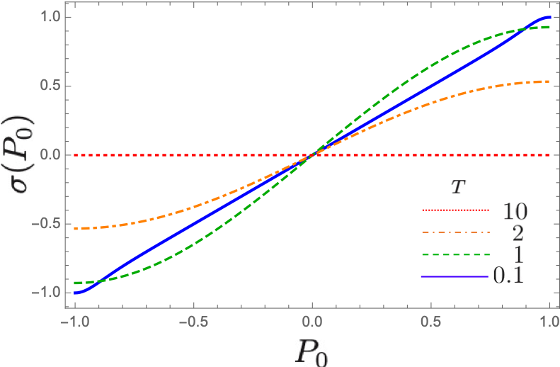
Figure 1: Momentum dependence of the sound velocity of a hydrodynamic mode of the exciton at temperatures $T=0.1$(solid), $1$(dashed),$2$(dash-dotted), $10$(dotted) in units where $m=1,c=1,\hbar=1,k_{{\rm B}}=1$.

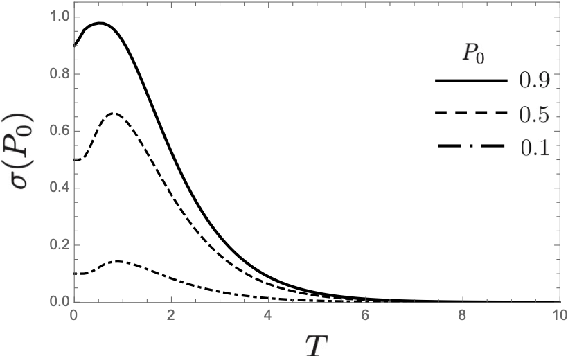
Figure 2: Temperature dependence of the sound velocity of a hydrodynamic mode of the exciton for momenta $P_{0}=0.9$ (solid), $0.5$ (dashed), $0.1$ (dash-dotted) in units where $m=1,c=1,\hbar=1,k_{{\rm B}}=1$.

In Figs. 1 and 2, we show the momentum dependence and the temperature dependence of the sound velocity (67).

In these figures, we show the results for our interesting temperature domain $1\lesssim k_{{\rm B}}T/mc^{2}\lesssim 2$, in addition to the temperature domain at lower and higher temperatures.

Note that the temperatures $k_{{\rm B}}T/mc^{2}=0.1$, $1$, $2$ and $10$ correspond to $T\simeq 22{\rm K}$, $220{\rm K}$, $440{\rm K}$ and $2200{\rm K}$, respectively. It can be confirmed that the sound velocity is the largest at $P_{0}/mc=1$ and it goes to zero at high temperatures as shown in Eq. (73). Furthermore, Fig. 2 shows that the sound velocity has relatively large values in the temperature domain $1\lesssim k_{{\rm B}}T/mc^{2}\lesssim 2$. As a result, one can readily see the momentum dependence of the sound velocity in this temperature domain.

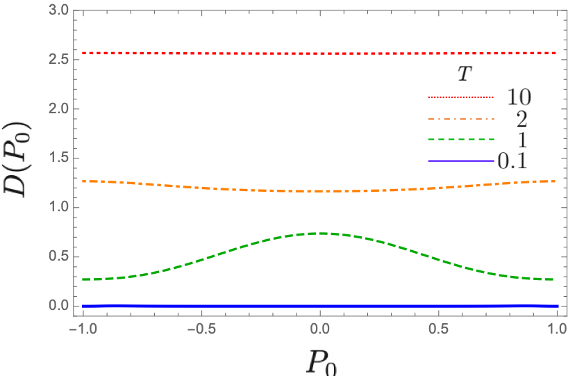
Figure 3: Momentum dependence of the diffusion coefficient of the exciton at temperatures $T=0.1$(solid), $1$(dashed),$2$(dash-dotted), $10$(dotted) in units where $m=1,c=1,\hbar=1,k_{{\rm B}}=1\ {\rm and}\ |\lambda_{\infty}|=1$.

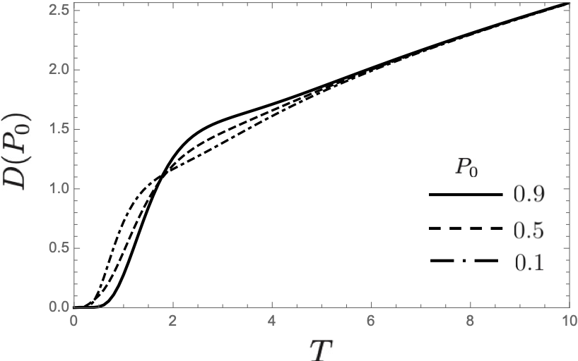
Figure 4: Temperature dependence of the diffusion coefficient of the exciton for momenta $P_{0}=0.9$ (solid), $0.5$ (dashed), $0.1$ (dash-dotted) in units where $m=1,c=1,\hbar=1,k_{{\rm B}}=1\ {\rm and}\ |\lambda_{\infty}|=1$.

Let us now consider the diffusion coefficient (62) expressed in terms of the nonzero eigenvalues $z_{P_{0};j}$ and corresponding right eigenvectors $\phi_{P_{0};j}(P_{\nu})$ of the collision operator ${\cal K}_{P}^{(0)}$. In this paper, we present the results obtained by the numerical calculation for these eigenvalues and the eigenvectors. The analytic form of the solution of the eigenvalue problem will be presented elsewhere. Here, we show the numerical results for the momentum dependence and the temperature dependence of the diffusion coefficient (62) in Figs. 3 and 4.

It is found that the momentum dependence of the diffusion coefficient is significant in the temperature domain of our our interest $1\lesssim k_{{\rm B}}T/mc^{2}\lesssim 2$ (see Fig. 3). For extremely high and low temperatures, the momentum dependence is no significant.

B. Convection-diffusion equation

In this section, we consider the time evolution of the Wigner distribution function for the exciton, and drive the convection-diffusion equation.

Since the collision operator is defined in each disjoint subspace associated with a subset of momenta, the time evolution of the distribution function is also determined for each disjoint subspace. The time evolution of the Fourier component of the Wigner distribution function $f_{k}(P_{\nu},t)$ that belongs to a certain momentum subset represented by $P_{0}$ is given by the eigenfunction expansion method as

$$f_{k}(P_{\nu},t)=\sum_{j}e^{-iz_{P_{0};j}^{(k)}t}\phi_{P_{0};j}^{(k)}(P_{\nu})\langle\!\langle\tilde{\phi}_{P_{0};j}^{(k)}|f(t=0)\rangle\!\rangle,$$ (74)

where

$$\langle\!\langle\tilde{\phi}_{P_{0};j}^{(k)}|f(t=0)\rangle\!\rangle=\sum_{\mu=-\infty}^{\infty}\tilde{\phi}_{P_{0};j}^{(k)}(P_{\mu})f_{k}(P_{\mu},0).$$ (75)

Eqs. (74) and (75) are the functions defined for each value of $P_{0}$. However, since $P_{\nu}$ and $P_{\mu}$ take any real number when $P_{0}$ varies continuously in the domain $-mc\leq P_{0}\leq mc$, the function $f_{k}(P,t)$ is defined to be a continuous function of $P$.

After the momentum relaxation $t\gtrsim\tau_{{\rm rel}}$, the system has reached the local equilibrium,

$$f_{k}(P,t) \xrightarrow{t\gtrsim\tau_{{\rm rel}}}e^{-iz_{P;0}^{(k)}t}\phi_{P;0}^{(k)}(P)\langle\!\langle\tilde{\phi}_{P;0}^{(k)}|f(t=0)\rangle\!\rangle.$$ (76)

In the hydrodynamic regime (54), the function $f_{k}(P,t)$ is expressed as

$$f_{k}(P,t\gtrsim\tau_{{\rm rel}})\simeq e^{-ik\sigma(P)t}e^{-k^{2}D(P)t}\phi_{P;0}^{(k)}(P)\langle\!\langle\tilde{\phi}_{P;0}^{(k)}|f(t=0)\rangle\!\rangle,$$ (77)

where $z_{P;0}^{(k)}$ is approximated up to the second-order of $k$ in Eq. (58). The Wigner distribution function for the exciton defined by Eq. (22) in the hydrodynamic regime is then given by

$$f^{W}(X,P,t\gtrsim\tau_{{\rm rel}})\simeq\frac{1}{2\pi}\int_{-\infty}^{\infty}\!\!\!\!dk\ e^{ik(X-\sigma(P)t)}e^{-k^{2}D(P)t}\phi_{P;0}^{(k)}(P)\langle\!\langle\tilde{\phi}_{P;0}^{(k)}|f(t=0)\rangle\!\rangle.$$ (78)

Differentiating this expression with respect to $X$ and $t$, we then obtain a convection-diffusion equation for $t\gtrsim\tau_{{\rm rel}}$ with a sound velocity $\sigma(P)$ and a diffusion coefficient $D(P)$ as

$$\frac{\partial}{\partial t}f^{W}(X,P,t)=-\sigma(P)\frac{\partial}{\partial X}f^{W}(X,P,t)+D(P)\frac{\partial^{2}}{\partial X^{2}}f^{W}(X,P,t).$$ (79)

We note that the effects of the sound velocity and the momentum dependence of the diffusion coefficient are significant. However, this convection-diffusion equation reduces to the usual diffusion equation for a high temperature, since the sound velocity is almost zero and the diffusion coefficient reaches a constant that does not depend on momentum at a high temperature.

IV phenomenological diffusion coefficient

In this section, we consider the phenomenological diffusion coefficient $D^{(x)}(t)$ in Eq. (1). In that expression, the symbol $\langle\cdots\rangle_{t}$ indicates to take the average over the Wigner distribution function $f^{W}(X,P,t)$ as

$$\langle g(X,P)\rangle_{t} \equiv\int_{-\infty}^{\infty}\!\!\!\!\!\!\!dX\int_{-\infty}^{\infty}\!\!\!\!\!\!\!dP\ g(X,P)\ f^{W}\!(X,P,t)$$

$$=\int_{-\infty}^{\infty}\!\!\!\!\!\!\!dX\int_{-mc}^{mc}\!\!\!\!\!\!\!\!dP_{0}\sum_{\nu=-\infty}^{\infty}\ g(X,P_{\nu})\ f^{W}\!(X,P_{\nu},t),$$ (80)

where $g(X,P)$ is an arbitrary function of $X$ and $P$. The integration over $P$ can be replaced with the integration of $P_{0}$ from $-mc$ to $mc$ after the summation over all the discrete momenta $P_{\nu}$ connected to each $P_{0}$.

As explained in the introduction, there is a numerical result reported by Pouthier 2009VPouthier that the phenomenological diffusion coefficient (1) for the exciton increases linearly with time and diverges in the long-time limit. We now show that the linear time dependence of $D^{(x)}(t)$ can be understood using an analytic expression for $D^{(x)}(t)$ in terms of the transport coefficients in the kinetic equation, and that the divergence of $D^{(x)}(t)$ in the long-time limit is due to the phase mixing which arises from the momentum dependence of the sound velocity.

In order to show this, we first consider a special case where the initial condition is given by a pure state associated to a wave function with the minimum uncertainty

$$\psi_{0}(X)=\left[\frac{1}{2\pi(\Delta X)^{2}}\right]^{\frac{1}{4}}\exp\left[i\frac{P^{\prime}}{\hbar}X-\frac{X^{2}}{4(\Delta X)^{2}}\right],$$ (81)

where $P^{\prime}$ is a peak position of the initial momentum distribution. We note that Pouthier gave an initial condition as a delta function of $X$. Therefore, his initial condition corresponds to the case $\Delta X\rightarrow 0$ in our initial condition.

For this state (81), the Fourier component of the Wigner distribution function at $t=0$ is given by (see Eq. (18))

$$f_{k}(P,t=0) =\left(P+\frac{\hbar k}{2}\right|f(0)\left|P-\frac{\hbar k}{2}\right)$$

$$=\left(P+\frac{\hbar k}{2}\middle|\psi_{0}\right)\left(\psi_{0}\middle|P-\frac{\hbar k}{2}\right)$$

$$=\frac{1}{\sqrt{2\pi(\Delta P)^{2}}}\exp\left[-\frac{(P-P^{\prime})^{2}}{2(\Delta P)^{2}}-\frac{(\Delta X)^{2}}{2}k^{2}\right],$$ (82)

where

$$\Delta X\cdot\Delta P=\hbar/2.$$ (83)

Substituting Eq. (82) into Eqs. (75) and (77), we obtain the Fourier component of the Wigner distribution function for $t\gtrsim\tau_{{\rm rel}}$ as

$$f_{k}(P_{\nu},t\gtrsim\tau_{{\rm rel}})\simeq e^{-\{ik\sigma(P_{0})+k^{2}D(P_{0})\}t}\phi_{P_{0};0}^{(k)}(P)\sum_{\mu=-\infty}^{\infty}\tilde{\phi}_{P_{0};0}^{(k)}(P_{\mu})\frac{1}{\sqrt{2\pi(\Delta P)^{2}}}\exp\left[-\frac{(P_{\mu}-P^{\prime})^{2}}{2(\Delta P)^{2}}-\frac{(\Delta X)^{2}}{2}k^{2}\right].$$ (84)

Then, we approximate $\phi_{P_{0};0}^{(k)}(P)$ and $\tilde{\phi}_{P_{0};0}^{(k)}(P)$ by the eigenfunctions in the $k=0$ subspace $\phi_{P_{0};0}(P)$ and $\tilde{\phi}_{P_{0};0}(P)$, respectively, for the hydrodynamic case with a small value of $k$ (see Eqs. (59)), and obtain

$$f_{k}(P_{\nu},t\gtrsim\tau_{{\rm rel}})\simeq e^{-\{ik\sigma(P_{0})+k^{2}D(P_{0})\}t}\varphi_{P_{0}}^{{\rm eq}}(P_{\nu})\sum_{\mu=-\infty}^{\infty}\frac{1}{\sqrt{2\pi(\Delta P)^{2}}}\exp\left[-\frac{(P_{\mu}-P^{\prime})^{2}}{2(\Delta P)^{2}}-\frac{(\Delta X)^{2}}{2}k^{2}\right],$$ (85)

where we have used the relations (65) and (108). We note that is a mixed state in spite of the fact that the initial condition was a pure state.

By performing a Fourier transform on Eq. (85), the time evolution of the Wigner distribution function for $t\gtrsim\tau_{{\rm rel}}$ is obtained as

$$\begin{split}f^{W}(X,P_{\nu},t\gtrsim\tau_{{\rm rel}})&=\frac{\exp\left(-\frac{P_{\nu}^{2}}{2mk_{{\rm B}}T}\right)}{\sum_{\kappa=-\infty}^{\infty}\exp\left(-\frac{P_{\kappa}^{2}}{2mk_{{\rm B}}T}\right)}\sum_{\mu=-\infty}^{\infty}\frac{1}{\sqrt{2\pi(\Delta P)^{2}}}\exp\left[-\frac{(P_{\mu}-P^{\prime})^{2}}{2(\Delta P)^{2}}\right]\\ &\times\frac{1}{\sqrt{2\pi\{(\Delta X)^{2}+2D(P_{0})t\}}}\exp\left[-\frac{(X-\sigma(P_{0})t)^{2}}{2\{(\Delta X)^{2}+2D(P_{0})t\}}\right],\end{split}$$ (86)

where $P_{\nu}$, $P_{\mu}$ and $P_{\kappa}$ are discrete momenta belonging to the subset of momenta represented by $P_{0}$.

Now we can calculate the average $\langle\cdots\rangle_{t}$ in Eq. (1). Since the initial spatial distribution is given as a Gaussian, one can integrate over $X$ by using the formula for the Gaussian integral. After the integration over $X$, the phenomenological diffusion coefficient (1) can be expressed as Eq. (2) (see Appendix B for a derivation). The explicit form of the averages $\langle\cdots\rangle_{\rm eq}$ in Eq. (2) are given by (129) and (130).

Furthermore, in this specific system, the averages $\langle\cdots\rangle_{\rm eq}$ of the transport coefficients are equal to the averages of them over the initial Wigner distribution function, such as,

$$\bigl{\langle}D(P)\bigr{\rangle}_{\rm eq} =\bigl{\langle}D(P)\bigr{\rangle}_{t=0},$$

$$\bigl{\langle}\sigma(P)\bigr{\rangle}_{\rm eq} =\bigl{\langle}\sigma(P)\bigr{\rangle}_{t=0}.$$ (87)

The reason that Eqs. (87) satisfy is as follows: Relaxation of momentum distribution occurs only among the momenta in each subset, and hence the sum of the momentum distribution probability within each subspace is conserved during the momentum equilibration. Besides, values of the transport coefficients $\sigma(P_{0})$ and $D(P_{0})$ are shared by the momenta in the subset connected to the momentum $P_{0}$ via the collision operator. Therefore, the average of the transport coefficients in each momentum subspace is conserved during the momentum equilibration.

For more general initial condition, one can obtain $D^{(x)}(t)$ as Eq. (2) with a time-independent extra term which comes from the deviation of the initial distribution from Gaussian. The proof is given in Appendix C, where we use the theorem that any square integrable function can be approximated with arbitrary precision by the linear combination of Gaussian 2008CCalcaterra ; 2008CCalcaterraABoldt .

The expression Eq. (2) shows that the phenomenological diffusion coefficient (1) consists of the two parts: the first term is due to the diffusion process and the second term is due to the phase mixing. The diffusion process is an irreversible process associated with entropy production. On the other hand, the phase mixing is a reversible process in which the wave packet spreads along the spatial direction in the phase space because of the difference of the sound velocity according to momentum. Therefore, the spreading of the spacial distribution occurs owing to completely different two mechanisms. The divergence of the phenomenological diffusion coefficient (1) is ascribed to the phase mixing.

In Fig. 5 is shown the time evolution of the Wigner distribution function (86) for $t>\tau_{\rm rel}$. The distribution in Fig. 5(a) has side peaks at $P_{1}/mc=1.5$ and $P_{-1}/mc=-2.5$ besides the main peak at $P_{0}/mc=P^{\prime}/mc=0.5$. This is because the exciton can make transitions only within the momentum subset (53) connected to the initial momenta.

After the equilibrium state for the momentum is established, the components of the Wigner distribution function at momenta (53) connecting to a $P_{0}$ move with the same velocity $\sigma(P_{0})$. Moreover, for those momenta the variance along the $X$-axis increases at the same rate of the diffusion coefficient $D(P_{0})$.

In Fig. 6, we show the components of the Wigner distribution function at the momenta connecting to a $P_{0}/mc=0.5$ and their projection onto the plane perpendicular to the $P$-axis. Those figures illustrate the fact that these momenta belonging to the same momentum subset share the same hydrodynamic sound velocity and the same diffusion coefficient.

We show in Fig. 7 the cross sections of the components of the Wigner distribution function at momenta belonging to different momentum subset. One can see that the diffusion processes broaden the variances of each cross sections with rates of the different diffusion coefficients. In addition, the difference between the peak positions of each cross sections increases with time since these cross sections of components of the Wigner distribution function move with different sound velocities associated with the different value of the momentum.

Hence if we observe the spatial distribution of the exciton defined by

$$f(X,t)\equiv\int_{-\infty}^{\infty}f^{W}(X,P,t)dP,$$ (88)

this function spreads in time not only due to the diffusion processes but also due to the effect of the phase mixing.

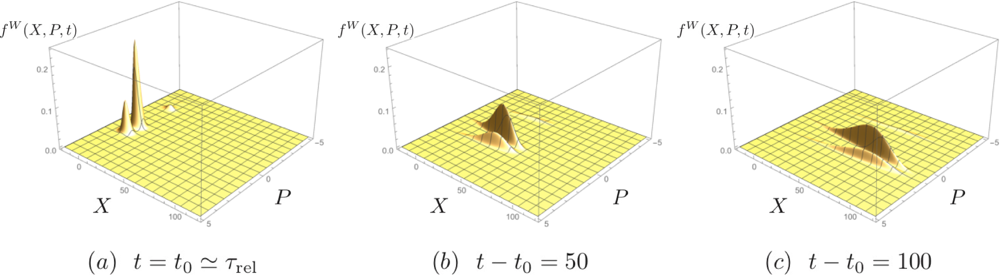
Figure 5: Time evolution of the Wigner distribution function for the exciton for $T=1$, $\Delta X=3$, $P^{\prime}=0.5$ in units where $m=1,c=1,\hbar=1,k_{{\rm B}}=1\ {\rm and}\ |\lambda_{\infty}|=1$.

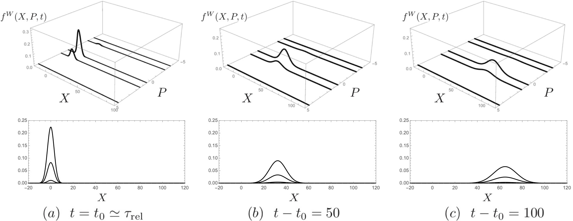
Figure 6: Cross sections of the Wigner distribution function for the exciton shown in Fig. 5 at $P_{0}=0.5$ in units where $m=1,c=1,\hbar=1,k_{{\rm B}}=1\ {\rm and}\ |\lambda_{\infty}|=1$. Each section moves with a same velocity $\sigma(P_{0}=0.5)$. The variances along $X$-axis increase at a same rate of a diffusion coefficient $D(P_{0}=0.5)$.

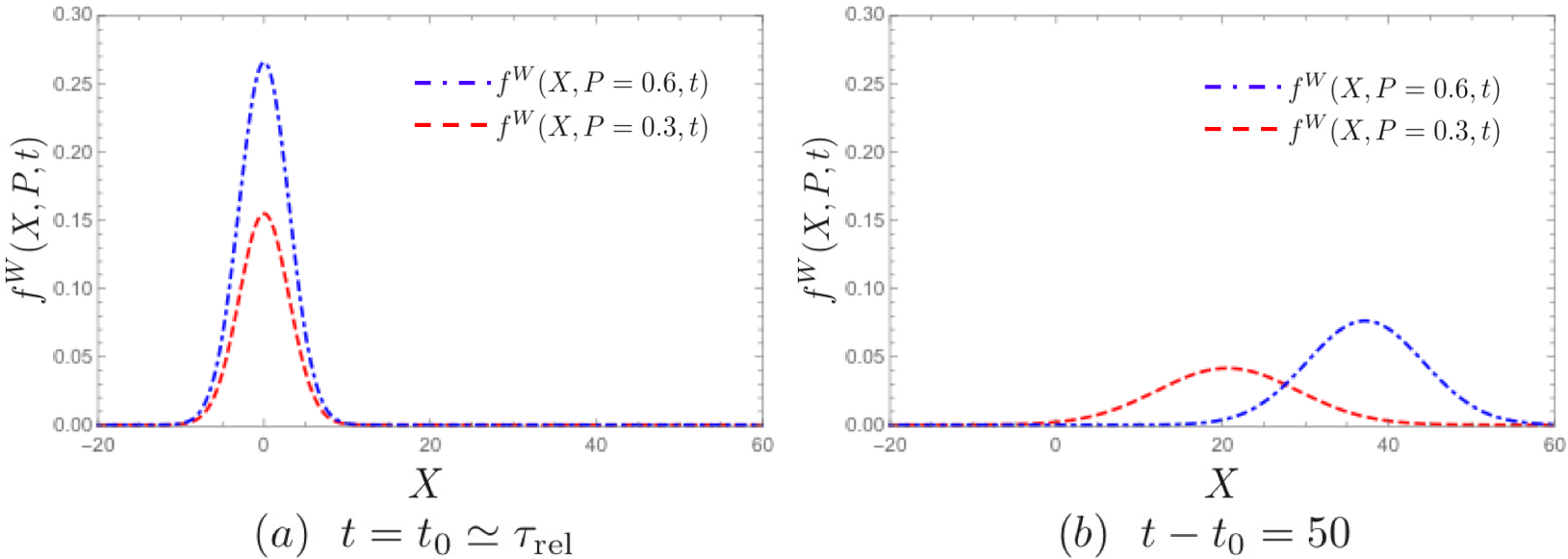
Figure 7: Cross sections of the Wigner distribution function for the exciton shown in Fig. 5 at $P=0.3$(dash-dotted), $0.5$(dashed) which belong to different momentum subspaces. The units $m=1,c=1,\hbar=1,k_{{\rm B}}=1$ and $|\lambda_{\infty}|=1$ are used.

V Conclusions

We have shown that a hydrodynamic mode emerges in relaxation processes of an exciton weakly coupled with a thermal phonon field in a 1D molecular chain. We obtained the hydrodynamic mode in the formalism of the complex spectral analysis of the Liouvillian by treating the flow term in the effective Liouvillian as a perturbation to the collision term. The mode is featured by a sound velocity and a diffusion coefficient, both of which depend on the momentum of the exciton. As a result, hydrodynamic sound wave propagation and diffusive relaxation coexist, and the time evolution of the Wigner function of the exciton obeys the convection-diffusion equation. Phase mixing due to the momentum dependence of the sound velocity leads to anomalous diffusion in the sense that the increase rate of the mean-square displacement of the exciton increases linearly with time and diverges in the long-time limit as Eq. (2).

One-dimensionality is crucial in giving the system with the properties mentioned above. From constraints on the collision processes in 1D represented by the resonance condition, it follows that the momentum space separates into infinite sets of disjoint subspaces dynamically independent of one another. Consequently, momentum relaxation occurs only within each subspace toward the Maxwell distribution constrained within the subspace. Thus, the transport coefficients are defined in each irreducible subspace, and in this sense the sound velocity and the diffusion coefficient are momentum-dependent. As a result, although the phenomenological diffusion coefficient defined by Eq. (1) diverges in the long-time limit, the diffusion coefficient as the transport coefficient in the kinetic equation is well-defined.

Moreover, a novel mechanism is responsible for the nonvanishing of the hydrodynamic sound velocity in our 1D system. As is well known, in classical gas systems, the degeneracy of the collisional invariants associated with the zero eigenmodes of the collision operator is lifted by the flow term in the inhomogeneous kinetic equation resulting in macroscopic hydrodynamic modes such as a sound wave mode and a diffusion mode in the hydrodynamic regime 1975RBalescu ; 1977PResiboisMdeLeenery . On the other hand, the appearance of the hydrodynamic mode with nonvanishing sound velocity in our 1D system is not due to a degeneracy, but due to a property that equilibration of momentum distribution occurs separately in each subset of momenta. The momentum distribution function on one of the subsets, in general, is neither even nor odd, because only one of $P$ and $-P$ is in the subset, while the velocity of the exciton $P/m$ is an odd function of the momentum. Thus, the sound velocity, which is given by the average of the velocity of the exciton over the equilibrium momentum distribution on a subset of momenta (see Eq. (66)), is non-vanishing in our 1D system.

When it comes to systems in more than one dimensions, the separation of momenta into subsets does not occur because of the angular degrees of freedom in collision processes (see above Eq. (52)). As a result, the equilibrium momentum distribution function is an even function. Hence, the sound velocity vanishes for systems in more than one dimensions.

Some authors have already pointed out that the phenomenological diffusion coefficient defined by Eq. (1) has a linear term with respect to time 1996HDoldererMWagner ; 1998HDoldererMWagner ; 2009VPouthier . However, it appears that in those situations the time-dependence of the phenomenological diffusion coefficient comes from phase mixing in free-particle like motion possibly with renormalization of the mass (polaron effect), because resonance with phonons is not effective for excitons with narrow excitation energy bandwidth treated in the papers. Note that phase mixing in free particle motion may occur also in higher spatial dimensions, in contrast to the fact that phase mixing due to the momentum-dependent sound velocity of the hydrodynamic mode appears only in 1D, as we have discussed in the present paper.

Finally, we emphasize the importance of the effects from the environment at finite temperatures in understanding the behavior of biological systems. We hope to clarify the role played by the hydrodynamic mode with non-vanishing sound velocity in bio-energy transfer processes in the future study.

Appendix A Relaxation modes of the momentum distribution function

In this appendix, we summarize the time evolution of the momentum distribution function of the exciton given by

$$f_{0}(P,t)\equiv\langle\!\langle 0,P|f(t)\rangle\!\rangle=(P|f(t)|P),$$ (89)

presented in our previous papers 2010KKankiSTanakaBATayTPetrosky ; 2011BATayKKankiSTanakaTPetrosky for the weak-coupling case. For details, refer to these papers.

The kinetic equation for the momentum distribution function of the exciton is written as

$$i\frac{\partial}{\partial t}{\cal P}^{(0)}|f(t)\rangle\!\rangle=\overline{\Psi}_{2}^{(0)}(i0^{+}){\cal P}^{(0)}|f(t)\rangle\!\rangle,$$ (90)

where the collision operator $\overline{\Psi}_{2}^{(0)}(i0^{+})$ is defined by Eq. (42). The notation ${\cal P}^{(0)}$ in Eq. (90) denotes the projection operator to the space spanned by the diagonal elements of the exciton density matrix with respect to the momentum states, and defined as

$${\cal P}^{(0)}\equiv\int dP|0,P\rangle\!\rangle\langle\!\langle 0,P|.$$ (91)

By multiplying $\langle\!\langle 0,P|$ from the left of Eq. (90), we obtain

$$i\frac{\partial}{\partial t}f_{0}(P,t)={\cal K}_{P}^{(0)}f_{0}(P,t),$$ (92)

where ${\cal K}_{P}^{(0)}$ is a difference operator given as Eq. (49).

Taking into account the consequences of the resonance condition in the collision operator (49), the kinetic equation (92) reduces to a difference equation, which can be written in a standard form of Markov master equation with gain and loss terms as

$$i\frac{\partial}{\partial t}f_{0}(P,t)=\!\!\!\sum_{P^{\prime}=-P\pm 2mc}\!\!\!\left\{K_{P,P^{\prime}}f_{0}(P^{\prime},t)-K_{P^{\prime},P}f_{0}(P,t)\right\},$$ (93)

where the sum on the right-hand side is the sum of the two cases, $P^{\prime}=-P+2mc$ and $P^{\prime}=-P-2mc$, and the transition probabilities $K_{P,P^{\prime}}/i$ are given by

$$-iK_{P,P^{\prime}}\equiv\frac{g^{2}m\Delta_{0}^{2}}{\hbar^{2}\rho_{M}c}\frac{1}{|\exp[(\varepsilon_{P}-\varepsilon_{P^{\prime}})/k_{\mathrm{B}}T]-1|}.$$ (94)

Now, we consider the eigenvalue problem of the collision operator,

$${\cal K}_{P}^{(0)}\phi_{j}(P)=z_{j}\phi_{j}(P).$$ (95)

The collision operator ${\cal K}_{P}^{(0)}$ is non-Hermitian operator. Thus, we have to consider the so-called right and left eigenvalue problem of the collision operator respectively. Since their eigenvalue equations consist of components with discrete momenta related to a $P_{0}$, the right and left eigenvectors are expressed with the discrete set of momenta (53) as

$$\langle\!\langle 0,P|\phi_{P_{0};j}\rangle\!\rangle \equiv\sum_{\nu}\phi_{P_{0};j}(P_{\nu})\delta(P-P_{\nu}(P_{0})),$$ (96)

$$\langle\!\langle\tilde{\phi}_{P_{0};j}|0,P\rangle\!\rangle \equiv\sum_{\nu}\tilde{\phi}_{P_{0};j}(P_{\nu})\delta(P-P_{\nu}(P_{0})),$$ (97)

where the expression $P_{\nu}(P_{0})$ indicates that $P_{\nu}$ is connected as Eq. (53) to a particular $P_{0}$ .We also introduce a representation of the eigenvectors $|\phi_{j}\rangle\!\rangle_{P_{0}}$ and ${}_{P_{0}}\langle\!\langle\tilde{\phi}_{j}|$ as vectors with components on a discrete set of momenta (53)

$${}_{P_{0}}\langle\!\langle 0,P_{\nu}|\phi_{j}\rangle\!\rangle_{P_{0}} \equiv\phi_{P_{0};j}(P_{\nu}),$$ (98)

$${}_{P_{0}}\langle\!\langle\tilde{\phi}_{j}|0,P_{\nu}\rangle\!\rangle_{P_{0}} \equiv\tilde{\phi}_{P_{0};j}(P_{\nu}),$$ (99)

with the basis vectors $|0,P_{\nu}\rangle\!\rangle_{P_{0}}$ and ${}_{P_{0}}\langle\!\langle 0,P_{\nu}|$ satisfying

$${}_{P_{0}}\langle\!\langle 0,P_{\mu}|0,P_{\nu}\rangle\!\rangle_{P_{0}}=\delta_{\mu,\nu}^{{\rm Kr}}.$$ (100)

The right-eigenvalue equation among the components $\phi_{P_{0};j}(P_{\nu})$ can be written as a set of equations,

$$-(K_{\nu+1,\nu}+K_{\nu-1,\nu})\phi_{P_{0};j}(P_{\nu})+K_{\nu,\nu-1}\phi_{P_{0};j}(P_{\nu-1})+K_{\nu,\nu+1}\phi_{P_{0};j}(P_{\nu+1})=z_{P_{0};j}\phi_{P_{0};j}(P_{\nu}),$$ (101)

where $\nu=0,\pm 1,\pm 2,\cdots,$ and $K_{\nu,\mu}\equiv K_{P_{\nu}P_{\mu}}$. The component $\phi_{P_{0};j}(P_{\nu})$ is the $j$-th right eigenvector on the set of momenta $P_{\nu}$ with a fixed $P_{0}$. It is clear that the eigenvalues depend on $P_{0}$ since the eigenvalue equations are determined for each momentum subspace connected to $P_{0}$. Similarly, the left eigenvalue equation among the components $\tilde{\phi}_{P_{0};j}(P_{\nu})$ of the $j$-th left eigenvector can be written as

$$\tilde{\phi}_{P_{0};j}(P_{\nu})\{-(K_{\nu+1,\nu}+K_{\nu-1,\nu})\}+\tilde{\phi}_{P_{0};j}(P_{\nu-1})K_{\nu,\nu-1}+\tilde{\phi}_{P_{0};j}(P_{\nu+1})K_{\nu,\nu+1}=z_{P_{0};j}\tilde{\phi}_{P_{0};j}(P_{\nu}).$$ (102)

The left and right eigenvector satisfy following relation,

$$\tilde{\phi}_{P_{0};j}(P_{\nu})=[\varphi_{P_{0}}^{{\rm eq}}(P_{\nu})]^{-1}\phi_{P_{0};j}(P_{\nu}),$$ (103)

where $\varphi_{P_{0}}^{{\rm eq}}(P)$ is given by Eq. (57)

The relationship (103) can be easily proved with Eqs. (101) and (102) by using the fact that the following detailed balance condition is satisfied:

$$K_{PP^{\prime}}\cdot\varphi^{{\rm eq}}(P^{\prime})=K_{P^{\prime}P}\cdot\varphi^{{\rm eq}}(P).$$ (104)

Keeping the relation (103), the right eigenvectors $\phi_{P_{0};j}(P_{\nu})$ and the left eigenvectors $\tilde{\phi}_{P_{0};j}(P_{\nu})$ can be made to satisfy the bi-orthonormality and bi-completeness relations,

$$\sum_{\nu=-\infty}^{\infty}\tilde{\phi}_{P_{0};j}(P_{\nu})\phi_{P_{0};j^{\prime}}(P_{\nu}) =\delta_{j,j^{\prime}}^{{\rm Kr}},$$ (105)

$$\sum_{\nu=-\infty}^{\infty}\tilde{\phi}_{P_{0};j}(P_{\mu})\phi_{P_{0};j}(P_{\nu}) =\delta_{\mu,\nu}^{{\rm Kr}}.$$ (106)

In particular, the right and left eigenvectors with zero eigenvalue are

$$\phi_{P_{0};0}(P_{\nu})=\varphi_{P_{0}}^{{\rm eq}}(P_{\nu}),$$ (107)

and

$$\tilde{\phi}_{P_{0};0}(P_{\nu})=1,$$ (108)

respectively. Note that

$$\sum_{\nu=-\infty}^{\infty}\phi_{P_{0};0}(P_{\nu})=\sum_{\nu=-\infty}^{\infty}\varphi_{P_{0}}^{\mathrm{eq}}(P_{\nu})=1,$$ (109)

see Eq.(57).

It can be shown that the collision operator (49) is anti-Hermitian with respect to an inner product weighted by $[\varphi_{P_{0}}^{{\rm eq}}(P_{\nu})]^{-1}$. For this point see Ref. 2011KKankiSTanakaTPetrosky . Hence the eigenvalues of the collision operator (49) are pure imaginary. Thus, we rewrite the eigenvalues of the collision operator in Eq. (95) as

$$z_{P_{0};j}=i\lambda_{P_{0};j},$$ (110)

where $\lambda_{P_{0};j}\in\mathbb{R}$.

We solved the eigenvalue problem of the collision operator (95) by numerical diagonalization and continued fraction method. For the detailed treatments see Ref. 2010KKankiSTanakaBATayTPetrosky ; 2011BATayKKankiSTanakaTPetrosky .

Figure 8: The spectrum of ${\cal K}^{(0)}_{P}$ for the temperatures, $T=0.1,1,2,{\rm and},10$, and $P_{0}=0.5$ in units where $m=1,c=1,\hbar=1,k_{{\rm B}}=1\ {\rm and}\ |\lambda_{\infty}|=1$.

Figure 9: Momentum dependence of the spectrum of ${\cal K}^{(0)}_{P}$ when $T=1$. The vertical axis is the eigenvalues and the horizontal axis is $P_{0}$ in units of $m=1,c=1,\hbar=1,k_{{\rm B}}=1\ {\rm and}\ |\lambda_{\infty}|=1$.

The spectrum of ${\cal K}_{P}^{(0)}$ is obtained for each $P_{0}$ as described under Eq. (101). In. Fig. 8, we display the spectrum of ${\cal K}^{(0)}_{P}$ for several temperatures, where $P_{0}/mc=0.5$. It is found that the spectrum of ${\cal K}^{(0)}_{P}$ is discrete and that the spectrum has an accumulation point $\lambda_{\infty}$ given by

$$\lambda_{\infty}\equiv-\frac{g^{2}m\Delta_{0}^{2}}{\hbar^{2}\rho_{M}c},$$ (111)

i.e., infinitely many eigenvalues exist in an arbitrarily small neighborhood of $\lambda_{\infty}$. Thus, we can label the eigenvalues with all the integers in the following way:

$$\lambda_{P_{0};0} \equiv 0>\lambda_{P_{0};1}>\lambda_{P_{0};2}>\cdots>\lambda_{P_{0};j}>\cdots>\lambda_{\infty}>\cdots$$

$$\ \ \ \ \cdots>\lambda_{P_{0};-j}>\cdots>\lambda_{P_{0};-2}>\lambda_{P_{0};-1}>-\infty.$$ (112)

The eigenvalues labeled with $j\geq 0$ are the ones which are larger than $\lambda_{\infty}$, the eigenvalues labeled with $j<0$ are the ones which are less than $\lambda_{\infty}$, and ${\rm lim}_{j\rightarrow\pm\infty}\lambda_{P_{0};j}=\lambda_{\infty}$.

In Fig. 9, we display the momentum dependence of the spectrum of ${\cal K}^{(0)}_{P}$, where $k_{{\rm B}}T/mc^{2}=1$. The vertical axis is the eigenvalues measured in units of $|\lambda_{\infty}|$, and the horizontal axis is $P_{0}/mc$. There is a zero eigenvalue of the spectrum at each $P_{0}$. In other words, the collision operators on each momentum subset $P_{0}$ have a collisional invariant. Therefore, the zero eigenvalues of the collision operator ${\cal K}_{P}^{(0)}$ are infinitely degenerate. Moreover, it is found that the spectrum of the collision operator for the momentum distribution function has a finite gap between zero eigenvalues and the non-zero eigenvalues for any momentum $P_{0}$,

$$\lambda_{{\rm gap}}\equiv\lambda_{P_{0};0}-\lambda_{P_{0};1}=-\lambda_{P_{0};1}\neq 0.$$ (113)

This fact implies that there exists a definite time scale, i.e. the relaxation time,

$$\tau_{{\rm rel}}\equiv 1/\lambda_{{\rm gap}}={\rm finite},$$ (114)

in momentum relaxation process. Hence, the local equilibrium situation can be realized in this model.

Appendix B Derivation of the phenomenological diffusion coefficient with Gaussian initial condition

In this section, we derive Eq. (2) in case where the initial condition is given by a wave function with the minimum uncertainty.

We rewrite the Wigner distribution function (86) as

$$f^{W}(X,P_{\nu},t)=\varphi_{P_{0}}^{{\rm eq}}(P_{\nu})g_{P_{0}}(X,t),$$ (115)

where $\varphi_{P_{0}}^{{\rm eq}}(P_{\nu})$ is defined in Eq. (57), and

$$g_{P_{0}}(X,t)\equiv a(P_{0})G(X,P_{0},t),$$ (116)

with

$$a(P_{0}) \equiv\sum_{\mu=-\infty}^{\infty}\frac{1}{\sqrt{2\pi(\Delta P)^{2}}}\exp\left[-\frac{(P_{\mu}(P_{0})-P^{\prime})^{2}}{2(\Delta P)^{2}}\right],$$ (117)

and

$$G(X,P_{0},t)\equiv\frac{1}{\sqrt{2\pi\{(\Delta X)^{2}+2D(P_{0})t\}}}\exp\left[-\frac{(X-\sigma(P_{0})t)^{2}}{2\{(\Delta X)^{2}+2D(P_{0})t\}}\right].$$ (118)

The function $a(P_{0})$ is a sum of distribution probabilities of the initial momentum distribution within a momentum subspace represented by $P_{0}$.

Since the momentum state can transition only within each subspace due to the resonance condition in 1D, the sum of the distribution probabilities within each momentum subspace (117) is conserved during momentum equilibration. Therefore, the distribution along $P$ direction after establishing local equilibrium in phase space is expressed as the product of the weighting factor and momentum equilibrium distribution: $a(P_{0})\varphi_{P_{0}}^{{\rm eq}}(P_{\nu})$.

On the other hand, $G(X,P_{0},t=0)$ is the initial spatial distribution function given as a Gaussian.

The phenomenological diffusion coefficient (1) can be written down in two terms as

$$D^{(x)}(t)=\frac{1}{2}\frac{d}{dt}\left\{\langle X^{2}\rangle_{t}-\langle X\rangle_{t}^{2}\right\}.$$ (119)

By the definition of the average (See Eq. (80)), the first and second term of (119) can be calculated respectively as

$$\langle X^{2}\rangle_{t} =\int_{-mc}^{mc}\!\!\!\!\!\!\!\!dP_{0}\sum_{\nu=-\infty}^{\infty}a(P_{0})\varphi_{P_{0}}^{{\rm eq}}(P_{\nu})\int_{-\infty}^{\infty}\!\!\!\!\!\!\!\!dX\ X^{2}G(X,P_{0},t),$$ (120)

$$\langle X\rangle_{t}^{2} =\left\{\int_{-mc}^{mc}\!\!\!\!\!\!\!\!dP_{0}\sum_{\nu=-\infty}^{\infty}a(P_{0})\varphi_{P_{0}}^{{\rm eq}}(P_{\nu})\int_{-\infty}^{\infty}\!\!\!\!\!\!\!\!dX\ XG(X,P_{0},t)\right\}^{2}.$$ (121)

One can easily integrate over $X$ in both Eq. (120) and Eq. (121) by Gaussian integral, and obtains

$$\langle X^{2}\rangle_{t} =\int_{-mc}^{mc}\!\!\!\!\!\!\!\!dP_{0}\sum_{\nu=-\infty}^{\infty}a(P_{0})\varphi_{P_{0}}^{{\rm eq}}(P_{\nu})\left\{(\Delta X)^{2}+2D(P_{0})t+(\sigma(P_{0})t)^{2}\right\},$$ (122)

$$\langle X\rangle_{t}^{2} =\left\{\int_{-mc}^{mc}\!\!\!\!\!\!\!\!dP_{0}\sum_{\nu=-\infty}^{\infty}a(P_{0})\varphi_{P_{0}}^{{\rm eq}}(P_{\nu})\sigma(P_{0})t\right\}^{2}.$$ (123)

Substituting Eqs. (122) and (123) into Eq. (119), we obtain $D^{(x)}(t)$ as a linear function of time:

$$D^{(x)}(t) =\int_{-mc}^{mc}\!\!\!\!\!\!\!\!dP_{0}\sum_{\nu=-\infty}^{\infty}a(P_{0})\varphi_{P_{0}}^{{\rm eq}}(P_{\nu})D(P_{0})$$

$$\ \ \ +t\left[\int_{-mc}^{mc}\!\!\!\!\!\!\!\!dP_{0}\sum_{\nu=-\infty}^{\infty}a(P_{0})\varphi_{P_{0}}^{{\rm eq}}(P_{\nu})(\sigma(P_{0}))^{2}-\left\{\int_{-mc}^{mc}\!\!\!\!\!\!\!\!dP_{0}\sum_{\nu=-\infty}^{\infty}a(P_{0})\varphi_{P_{0}}^{{\rm eq}}(P_{\nu})\sigma(P_{0})\right\}^{2}\right].$$ (124)

Since the initial spatial distribution is given by the Gaussian, the equation

$$a(P_{0})=\int_{-\infty}^{\infty}\!\!\!\!\!\!\!\!dX\ g_{P_{0}}(X,t),$$ (125)

holds. Substituting Eq. (125) into each terms in Eq. (124), one can obtain the form of the average defined in Eq. (80) as

$$D^{(x)}(t) =\int_{-\infty}^{\infty}\!\!\!\!\!\!\!dX\int_{-mc}^{mc}\!\!\!\!\!\!\!\!dP_{0}\sum_{\nu=-\infty}^{\infty}D(P_{0})f^{W}(X,P_{\nu},t)$$

$$\ \ \ +t\left[\int_{-\infty}^{\infty}\!\!\!\!\!\!\!dX\int_{-mc}^{mc}\!\!\!\!\!\!\!\!dP_{0}\sum_{\nu=-\infty}^{\infty}(\sigma(P_{0}))^{2}f^{W}(X,P_{\nu},t)-\left\{\int_{-\infty}^{\infty}\!\!\!\!\!\!\!dX\int_{-mc}^{mc}\!\!\!\!\!\!\!\!dP_{0}\sum_{\nu=-\infty}^{\infty}\sigma(P_{0})f^{W}(X,P_{\nu},t)\right\}^{2}\right].$$ (126)

Therefore, we get

$$D^{(x)}(t)=\bigl{\langle}D(P)\bigr{\rangle}_{t}+t\left[\bigl{\langle}\sigma^{2}(P)\bigr{\rangle}_{t}-\bigl{\langle}\sigma(P)\bigr{\rangle}_{t}^{2}\right].$$ (127)

Then, we can integrate over $X$ in the averages in Eq. (127) and obtain

$$D^{(x)}(t) =\bigl{\langle}D(P)\bigr{\rangle}_{\rm eq}+t\left[\bigl{\langle}\sigma^{2}(P)\bigr{\rangle}_{\rm eq}-\bigl{\langle}\sigma(P)\bigr{\rangle}_{\rm eq}^{2}\right]$$

$$=\bar{D}+t\left\langle(\sigma(P)-\bar{\sigma})^{2}\right\rangle_{\rm eq},$$ (128)

where

$$\bar{D} =\bigl{\langle}D(P)\bigr{\rangle}_{\rm eq}\equiv\int_{-mc}^{mc}\!\!\!\!\!\!\!\!dP_{0}\sum_{\nu=-\infty}^{\infty}a(P_{0})\varphi_{P_{0}}^{{\rm eq}}(P_{\nu})D(P_{0}),$$ (129)

$$\bar{\sigma} =\bigl{\langle}\sigma(P)\bigr{\rangle}_{\rm eq}\equiv\int_{-mc}^{mc}\!\!\!\!\!\!\!\!dP_{0}\sum_{\nu=-\infty}^{\infty}a(P_{0})\varphi_{P_{0}}^{{\rm eq}}(P_{\nu})\sigma(P_{0}).$$ (130)

Let us prove that Eqs. (87) is satisfied. Using the relation (109), Eq. (129) can be reduced as

$$\bigl{\langle}D(P)\bigr{\rangle}_{\rm eq} =\int_{-mc}^{mc}\!\!\!\!\!\!\!\!dP_{0}\ a(P_{0})D(P_{0}).$$ (131)

Substituting Eq. (117) into Eq. (131), we get

$$\bigl{\langle}D(P)\bigr{\rangle}_{\rm eq}=$$

$$\int_{-mc}^{mc}\!\!\!\!\!\!\!\!dP_{0}\sum_{\mu=-\infty}^{\infty} \frac{1}{\sqrt{2\pi(\Delta P)^{2}}}\exp\left[-\frac{(P_{\mu}(P_{0})-P^{\prime})^{2}}{2(\Delta P)^{2}}\right]D(P_{0}).$$ (132)

Replacing the integration over $P_{0}$ and the summation over all the discrete momentum $P_{\mu}$ with an integration over $P$, we obtain

$$\bigl{\langle}D(P)\bigr{\rangle}_{\rm eq} =\int_{-\infty}^{\infty}\!\!\!\!\!\!\!\!dP\ \frac{1}{\sqrt{2\pi(\Delta P)^{2}}}\exp\left[-\frac{(P-P^{\prime})^{2}}{2(\Delta P)^{2}}\right]D(P)$$ (133)

$$=\bigl{\langle}D(P)\bigr{\rangle}_{t=0}.$$

Similarly, one can get the averages of the hydrodynamic sound velocity as

$$\bigl{\langle}\sigma(P)\bigr{\rangle}_{\rm eq} =\int_{-\infty}^{\infty}\!\!\!\!\!\!\!\!dP\ \frac{1}{\sqrt{2\pi(\Delta P)^{2}}}\exp\left[-\frac{(P-P^{\prime})^{2}}{2(\Delta P)^{2}}\right]\sigma(P)$$ (134)

$$=\bigl{\langle}\sigma(P)\bigr{\rangle}_{t=0}.$$

Appendix C phenomenological diffusion coefficient in arbitrary initial condition

In this section, we show that the phenomenological diffusion coefficient $D^{(x)}(t)$ defined as Eq. (1) increases linearly with time in a case where the initial condition is given as arbitrary square integrable function. To prove this we use a theorem shown by Calcaterra (2008CCalcaterra ; 2008CCalcaterraABoldt , Theorem 1). Here, we introduce the theorem.

$\textit{Definition}s$: $L^{2}(\mathbb{R})$ $denotes$ $the$ $space$ $of$ $square$ $integrable$ $functions$ $f$: $\mathbb{R}\rightarrow\mathbb{R}$ $with$ $norm$

$$||f||_{2}\equiv\sqrt{\int_{\mathbb{R}}|f(x)|^{2}dx}.$$

$Relation$ $f\underset{\epsilon}{\approx}g$ $means$ $||f-g||_{2}<\epsilon$.

Theorem 1: $For$ $any$ $f\in L^{2}(\mathbb{R})$ $and$ $any$ $\epsilon>0$ $there$ $exists$ $s>0$ , $N\in\mathbb{N}$ $and$ $a_{n}\in\mathbb{R}$ $such$ $that$

$$f\underset{\epsilon}{\approx}\sum_{n=0}^{N}a_{n}e^{-(x-ns)^{2}}.$$

Calcaterra gives one choice of coefficients as

$$a_{n}=\frac{1}{\sqrt{\pi}}\frac{(-1)^{n}}{n!}\sum_{k=n}^{N}\frac{1}{(k-n)!(2s)^{k}}\int_{\mathbb{R}}f(x)e^{x^{2}}\frac{d^{k}}{dx^{k}}e^{-x^{2}}dx.$$ (135)

We obtained the formal solution of Fourier component of the Wigner function belonging to a certain momentum subspace $P_{0}$ for $t\gtrsim\tau_{{\rm rel}}$ as (see Eq. (76) )

$$f_{k}(P_{\nu},t\gtrsim\tau_{{\rm rel}})=e^{-iz_{P_{0};0}^{(k)}t}\phi_{P_{0};0}^{(k)}(P_{\nu})\sum_{\mu=-\infty}^{\infty}\tilde{\phi}_{P_{0};0}^{(k)}(P_{\mu})f_{k}(P_{\mu},t=0).$$ (136)

We can approximate Eq. (136) in the hydrodynamic regime as mentioned at Eqs. (77) and (85),

$$f_{k}(P_{\nu},t\gtrsim\tau_{{\rm rel}}) \simeq e^{-ik\sigma(P_{0})t}e^{-k^{2}D(P_{0})t}\varphi_{P_{0}}^{{\rm eq}}(P_{\nu})\sum_{\mu=-\infty}^{\infty}f_{k}(P_{\mu},t=0).$$ (137)

Equation (137) is the formal solution of Fourier component of the Wigner distribution function after establishing local equilibrium in the hydrodynamic regime. We define the factor dependent on the initial distribution as

$$W_{P_{0}}(k)\equiv\sum_{\mu=-\infty}^{\infty}f_{k}(P_{\mu}(P_{0}),t=0).$$ (138)

The factor $W_{P_{0}}(k)$ is the function defined for each value of $P_{0}$.

By performing a Fourier transform on Eq. (137), we obtain the formal solution of the Wigner distribution function as

$$f^{W}(X,P_{\nu},t\gtrsim\tau_{{\rm rel}})=\varphi_{P_{0}}^{{\rm eq}}(P_{\nu})g_{P_{0}}(X,t),$$ (139)

where

$$g_{P_{0}}(X,t)\equiv\frac{1}{2\pi}\int_{-\infty}^{\infty}\!\!\!\!\!dk\ e^{ikX}e^{-ik\sigma(P_{0})t}e^{-k^{2}D(P_{0})t}W_{P_{0}}(k).$$ (140)

Equation (139) shows that the Wigner distribution function in a certain momentum subspace $P_{0}$ can be written in the form of the product of the momentum equilibrium distribution $\varphi_{P_{0}}^{{\rm eq}}(P_{\nu})$ and the spatial distribution (140).

Putting $t=0$ in Eq. (140), we get the initial spatial distribution function defined for each value of $P_{0}$ as

$$g_{P_{0}}(X,0)=\frac{1}{2\pi}\int_{-\infty}^{\infty}\!\!\!\!\!dk\ e^{ikX}W_{P_{0}}(k).$$ (141)

Here, we use Theorem 1. According to Theorem 1, any square integrable function can be approximated with arbitrary precision by the linear combination of Gaussians with a single variance. If we assume $g_{P_{0}}(X,0)$ as square integrable function, it can be expanded as [cf. Eq. (116)]

$$g_{P_{0}}(X,0)\underset{\epsilon}{\approx}\sum_{n=0}^{N}\frac{1}{\sqrt{2\pi}\Delta X}a_{n}(P_{0})e^{-(\frac{X}{\sqrt{2}\Delta X}-ns)^{2}},$$ (142)

where $\Delta X$ is a constant with a unit of length, and

$$a_{n}(P_{0})\equiv\frac{(-1)^{n}}{n!}\sum_{k=n}^{N}\frac{1}{(k-n)!(2s)^{k}}\int_{-\infty}^{\infty}g_{P_{0}}(X,0)e^{X^{2}}\frac{d^{k}}{dX^{k}}e^{-X^{2}}dX.$$ (143)

By inverse transformation of Eq. (141), we obtain

$$W_{P_{0}}(k)=\sum_{n=0}^{N}a_{n}(P_{0})\exp\left[-\frac{(\Delta X)^{2}}{2}k^{2}-i\sqrt{2}\Delta Xnsk\right].$$ (144)

Substituting Eq. (144) into Eq. (140) and integrating over $k$, we get spatial distribution function in a certain momentum subspace $P_{0}$ as

$$g_{P_{0}}(X,t)=\sum_{n=0}^{N}a_{n}(P_{0})\frac{1}{\sqrt{2\pi((\Delta X)^{2}+2D(P_{0})t)}}\exp\left[-\frac{(X-\sigma(P_{0})t-\sqrt{2}\Delta Xns)^{2}}{2\{(\Delta X)^{2}+2D(P_{0})\}t}\right].$$ (145)

We note that $g_{P_{0}}(X,t)$ is represented by a single term in the case where the initial distribution is given by one Gaussian as shown in Eq. (116).

Now we can calculate the phenomenological diffusion coefficient (1) with Eqs. (139) and (145). Since we got the spatial distribution $g_{P_{0}}(X,t)$ as the linear combination of Gaussians, we can integrate over $X$ by Gaussian integral. After simple calculation, the phenomenological diffusion coefficient $D^{(x)}(t)$ in a general case is finally expressed as

$$D^{(x)}(t)= \bar{D}+t\ \bigl{\langle}(\sigma(P)-\bar{\sigma})^{2}\bigr{\rangle}_{\rm eq}$$

$$+\bigl{\langle}\left(X-\langle X\rangle_{t=0})(\sigma(P)-\bar{\sigma}\right)\bigr{\rangle}_{t=0},$$ (146)

where the notation $\langle\cdots\rangle_{t=0}$ indicates to take average over the initial Wigner distribution function. Note that

$$\langle X\rangle_{t=0}\neq\langle X\rangle_{\rm eq}.$$ (147)

The averages of transport coefficients in Eq. (146) are expressed as [cf. Eq. (131)]

$$\bar{D}=\bigl{\langle}D(P)\bigr{\rangle}_{\rm eq}=\sum_{n=0}^{N}\int_{-mc}^{mc}\!\!\!\!\!\!\!dP_{0}\ a_{n}(P_{0})D(P_{0}),$$ (148)

$$\bar{\sigma}=\bigl{\langle}\sigma(P)\bigr{\rangle}_{\rm eq}=\sum_{n=0}^{N}\int_{-mc}^{mc}\!\!\!\!\!\!\!dP_{0}\ a_{n}(P_{0})\sigma(P_{0}).$$ (149)

Equation (146) shows that $D^{(x)}(t)$ increases linearly with time and diverges in the long-time limit. The third term in the right-hand side of Eq. (146) comes from the deviation of the initial distribution from Gaussian distribution. The third term vanishes in cases where the initial spatial distribution is given by one Gaussian distribution since the term is an integral of an odd function of $X$ in those cases. Under that condition, Eq. (146) therefore reduces to Eq. (127).