Improved Sleeping Bandits with Stochastic Actions Sets
and Adversarial Rewards

Abstract

In this paper, we consider the problem of sleeping bandits with stochastic action sets and adversarial rewards. In this setting, in contrast to most work in bandits, the actions may not be available at all times. For instance, some products might be out of stock in item recommendation. The best existing efficient (i.e., polynomial-time) algorithms for this problem only guarantee an $O(T^{2/3})$ upper-bound on the regret. Yet, inefficient algorithms based on EXP4 can achieve $O(\sqrt{T})$. In this paper, we provide a new computationally efficient algorithm inspired by EXP3 satisfying a regret of order $O(\sqrt{T})$ when the availabilities of each action $i\in{\mathcal{A}}$ are independent. We then study the most general version of the problem where at each round available sets are generated from some unknown arbitrary distribution (i.e., without the independence assumption) and propose an efficient algorithm with $O(\sqrt{2^{K}T})$ regret guarantee. Our theoretical results are corroborated with experimental evaluations.

1 Introduction

The problem of standard multiarmed bandit (MAB) is well studied in machine learning (Auer, 2000; Vermorel & Mohri, 2005) and used to model online decision-making problems under uncertainty. Due to their implicit exploration-vs-exploitation tradeoff, bandits are able to model clinical trials, movie recommendations, retail management job scheduling etc., where the goal is to keep pulling the ‘best-item’ in hindsight through sequentially querying one item at a time and subsequently observing a noisy reward feedback of the queried arm (Even-Dar et al., 2006; Auer et al., 2002a; Auer, 2002; Agrawal & Goyal, 2012; Bubeck et al., 2012). However, in various real world applications, the decision space (set of arms ${\mathcal{A}}$) often changes over time due to unavailability of some items etc. For instance, in retail stores some items might go out of stock, on a certain day some websites could be down, some restaurants might be closed etc. This setting is known as sleeping bandits in online learning (Kanade et al., 2009; Neu & Valko, 2014; Kanade & Steinke, 2014; Kale et al., 2016), where at any round the set of available actions could vary stochastically based on some unknown distributions over ${\mathcal{A}}$ (Neu & Valko, 2014; Cortes et al., 2019) or adversarially (Kale et al., 2016; Kleinberg et al., 2010; Kanade & Steinke, 2014). Besides the reward model, the set of available actions could also vary stochastically or adversarially (Kanade et al., 2009; Neu & Valko, 2014). The problem is known to be NP-hard when both rewards and availabilities are adversarial (Kleinberg et al., 2010; Kanade & Steinke, 2014; Kale et al., 2016). In case of stochastic rewards and adversarial availabilities the achievable regret lower bound is known to be $\Omega(\sqrt{KT})$, $K$ being the number of actions in the decision space ${\mathcal{A}}=[K]$. The well studied EXP$4$ algorithm does achieve the above optimal regret bound, although it is computationally inefficient (Kleinberg et al., 2010; Kale et al., 2016). However, the best known efficient algorithm only guarantees an $\tilde{O}((TK)^{2/3})$ regret, which is not matching the lower bound both in $K$ and $T$ (Neu & Valko, 2014).

In this paper we aim to give computationally efficient and optimal $O(\sqrt{T})$ algorithms for the problem of sleeping bandits with adversarial rewards and stochastic availabilities. Our specific contributions are as follows:

Contributions

• We identified a drawback in the (sleeping) loss estimates in the prior work for this setting and gave an insight and margin for improvement over the best know rate (Section 3).

• We first study the setting when the availabilities of each item $i\in{\mathcal{A}}$ are independent and propose an EXP$3$-based algorithm (Alg. 1) with an $O(K^{2}\sqrt{T})$ regret guarantee (Theorem 2, Sec. 3).

• We next study the problem when availabilities are not independent and give an algorithm with an $O(\sqrt{2^{K}T})$ regret guarantee (Sec. 4).

• We corroborated our theoretical results with empirical evidence (Sec. 5).

2 Problem Statement

Notation. We denote by $[n]:=\{1,2,\ldots,n\}$. ${\mathbf{1}}(\cdot)$ denotes the indicator random variable which takes value $1$ if the predicate is true and $0$ otherwise. $\tilde{O}(\cdot)$ notation is used to hide logarithmic dependencies.

2.1 Setup

Suppose the decision space (or set of actions) is $[K]:=\{1,2,\ldots,K\}$ with $K$ distinct actions, and we consider a $T$ round sequential game. At each time step $t\in[T]$, the learner is presented a set of available actions at round $t$, say $S_{t}\subseteq[K]$, upon which the learner’s task is to play an action $i_{t}\in S_{t}$ and consequently suffer a loss $\ell_{t}(i_{t})\in[0,1]$, where $\boldsymbol{\ell}_{t}:=[\ell_{t}(i)]_{i\in[K]}\in[0,1]^{K}$ denotes the loss of the $K$ actions chosen obliviously independent of the available actions $S_{t}$ at time $t$. We consider the following two types of availabilities:

Independent Availabilities. In this case we assume that the availability of each item $i\in[K]$ is independent of the rest $[K]\setminus\{i\}$, such that at each round item $i\in[K]$ is drawn in set $S_{t}$ with probability $a_{i}\in[0,1]$, or in other words, for all item $i\in[K]$, ${\mathbf{1}}(i\in S_{t})\sim Ber(a_{i})$, where availability probabilities $\{a_{i}\}_{i\in[K]}$ are fixed over time intervals $t$, independent of each other, and unknown to the learner.

General Availabilities. In this case each $S_{t}$s is drawn iid from some unknown distribution ${\mathcal{P}}$ over subsets $\{S\subseteq[K],|S|\geq 1\}$ with no further assumption made on the properties of ${\mathcal{P}}$. We denote by $P(S)$ the probability of occurrence of set $S$.

Analyses with independent and general availabilities are provided respectively in Sec. 3 and 4.

2.2 Objective

We define by a policy $\pi:2^{[K]}\mapsto[K]$ to be a mapping from a set of available actions/experts to an item.

Regret definition The performance of the learner, measured with respect to the best policy in hindsight, is defined as:

$$R_{T}=\max_{\pi:2^{[K]}\mapsto[K]}{\mathbf{E}}\bigg{[}\sum_{t=1}^{T}\ell_{t}(i_{t})-\sum_{t=1}^{T}\ell_{t}(\pi(S_{t}))\bigg{]},$$ (1)

where the expectation is taken w.r.t. the availabilities and the randomness of the player’s strategy.

Remark 1.

One obvious regret lower bound of the above objective is $\Omega(\sqrt{KT})$, which follows from the bound of standard MAB with adversarial losses (Auer et al., 2002a) for the special case when all the items are available at all times (even for availability-independent case). Interestingly, for a harder Sleeping-Bandits setting with adversarial availabilities the lower bound is $\Omega(K\sqrt{T})$ (Kleinberg et al., 2010), even for which no computationally efficient algorithm is known till date (EXP4 is the only algorithm which achieves the regret but it is computationally inefficient). Thus the interesting question to answer here is if for our setup–that lies in the middle-ground of (Auer et al., 2002a) and (Kleinberg et al., 2010)–is it possible to attend the $O(K\sqrt{T})$ learning rate? Here lies the primary objective of this work. To the best of our knowledge, there is no existing algorithm which are known to achieve this optimal rate and the best known efficient algorithm is only guaranteed to yield an $\tilde{O}((TK)^{2/3})$ regret (Neu & Valko, 2014).

3 Proposed algorithm: Independent Availabilities

In this section we propose our first algorithm for the problem (Sec. 2), which is based on a variant of thr EXP3 algorithm with a ‘suitable’ loss estimation technique. Thm. 2 proves the optimality of its regret performance.

Algorithm description. Similar to EXP$3$ algorithm, at every round $t\in[T]$ we maintain a probability distribution ${\mathbf{p}}_{t}$ over the arm set $[K]$ and also the empirical availability of each item $\widehat{a}_{ti}=\frac{1}{t}\sum_{\tau=1}^{t}{\mathbf{1}}(i\in S_{\tau})\,.$ Upon receiving the available set $S_{t}$, the algorithm redistributes ${\mathbf{p}}_{t}$ only on the set of available items $S_{t}$, say ${\mathbf{q}}_{t}$, and plays an item $i_{t}\sim{\mathbf{q}}_{t}$. Subsequently the environment reveals the loss $\ell_{t}(i_{t})$, and we update the distribution ${\mathbf{p}}_{t+1}$ using exponential weights on the loss estimates for all $i\in[K]$

$$\widehat{\ell}_{t}(i)=\frac{\ell_{t}(i){\mathbf{1}}(i=i_{t})}{\bar{q}_{t}(i)+\lambda_{t}}\,,$$ (2)

where $\lambda_{t}$ is a scale parameter and $\bar{q}_{t}(i)$ (see definition (3)) is an estimation of $Pr_{S_{t},i_{t}}\big{(}i_{t}=i\big{)}$, the probability of playing arm $i$ at time $t$ under the joint uncertainty in availability of $i$ (due to $S_{t}\sim{\mathcal{P}}$) and the randomness of EXP3 algorithm (due to $i_{t}\sim{\mathbf{p}}_{t}$).

New insight compared to existing algorithms. It is crucial to note that one of our main contributions lies in the loss estimation technique $\widehat{\boldsymbol{\ell}}_{t}$ in (2). The standard loss estimates used by EXP3 (see (Auer et al., 2002b)) are of the form $\widehat{\ell}_{t}(i)=\ell_{t}(i){\mathbf{1}}(i=i_{t})/p_{t}(i)$. Yet, because of the unavailable actions, the latter is biased. The solution proposed by (Neu & Valko, 2014) (see Sec. 4.3) consists of using unbiased loss estimates of the form $\widehat{\ell}_{t}(i)=\ell_{t}(i){\mathbf{1}}(i=i_{t})/(\widehat{p}_{t}(i)\widehat{a}_{ti})$ where $\widehat{a}_{ti}$ and $\widehat{p}_{t}(i)$ are estimates for the availability probability $a_{i}$ and for the weight $p_{t}(i)$ respectively. The suboptimal $O(T^{2/3})$ of their regret bound resulted from this separated estimation of $\widehat{p}_{t}(i)$ and $\widehat{a}_{ti}$, which leads to a high variance in the analysis because $\widehat{p}_{t}(i)=0$ whenever $i\notin S_{t}$.

We circumvent this problem by estimating them jointly as

$$\bar{q}_{t}(i):=\sum_{S\in 2^{[K]}}P_{\widehat{\mathbf{a}}}(S)q_{t}^{S}(i)\,,$$ (3)

where $P_{\widehat{\mathbf{a}}_{t}}(S)=\Pi_{i=1}^{K}\widehat{a}_{ti}^{{\mathbf{1}}(i\in S)}(1-\widehat{a}_{ti})^{1-{\mathbf{1}}(i\in S)}$ is the empirical probability of the availability of set $S$, and for all $i\in[K]$

$$q_{t}^{S}(i):=\frac{p_{t}(i){\mathbf{1}}(i\in S)}{\sum_{j\in S}p_{t}(j)},\,$$ (4)

is the redistributed mass of ${\mathbf{p}}_{t}$ on support set $S$. As shown in Lem. 1, $\bar{q}_{t}(i)$ is a good estimate for $q_{t}^{*}(i)={\mathbf{E}}_{S\sim{\mathbf{a}}}\big{[}q_{t}^{S}(i)\big{]}$, which is the conditional probability of playing action $i_{t}=i$ at time $t$. It turns out that $\bar{q}_{t}(i)$ is much more stable than $\widehat{p}_{t}(i)\widehat{a}_{ti}$ and therefore implies better variance control in the regret analysis. This improvement finally leads to the optimal $O(\sqrt{T})$ regret guarantee (Thm. 2). The complete algorithm is given in Alg. 1.

Algorithm 1 Sleeping-EXP3

1:  Input:

2:      Item set: $[K]$, learning rate $\eta$, scale parameter $\lambda_{t}$

3:      Confidence parameter: $\delta>0$

4:  Initialize:

5:      Initial probability distribution ${\mathbf{p}}_{1}(i)=\frac{1}{K},~{}\forall i\in[K]$

6:  while $t=1,2,\ldots$ do

7:     Define $q_{t}^{S}(i):=\frac{p_{t}(i){\mathbf{1}}(i\in S)}{\sum_{j\in S}p_{t}(j)},\,\forall i\in[K],S\subseteq[K]$

8:     Receive $S_{t}\subseteq[K]$

9:     Sample $i_{t}\sim{\mathbf{q}}_{t}^{S_{t}}$

10:     Receive loss $\ell_{t}(i_{t})$

11:     Compute: $\widehat{a}_{ti}=\frac{\sum_{\tau=1}^{t}{\mathbf{1}}(i\in S_{\tau})}{t}$

12:                  $P_{\widehat{\mathbf{a}}}(S)=\Pi_{i=1}^{K}\widehat{a}_{ti}^{{\mathbf{1}}(i\in S)}(1-\widehat{a}_{ti})^{1-{\mathbf{1}}(i\in S)}$

13:                  $\bar{q}_{t}(i)=\sum_{S\in 2^{[K]}}P_{\widehat{\mathbf{a}}}(S)q_{t}^{S}(i)$

14:     Estimate loss: $\widehat{\ell}_{t}(i)=\frac{\ell_{t}(i){\mathbf{1}}(i=i_{t})}{\bar{q}_{t}(i)+\lambda_{t}}$, $\forall i\in[K]$

15:     Update $p_{t+1}(i)=\frac{p_{t}(i)e^{-\eta\widehat{\ell}_{t}(i)}}{\sum_{j=1}^{K}p_{t}(i)e^{-\eta\widehat{\ell}_{t}(j)}},\,\forall i\in[K]$

16:  end while

The first crucial result we derive towards proving Thm. 2 is the following concentration guarantees on $\bar{q}_{t}$:

Lemma 1 (Concentration of $\bar{\mathbf{q}}_{t}$).

Let $t\in[T]$ and $\delta\in(0,1)$. Let $q^{*}_{t}(i)={\mathbf{E}}_{S\sim{\mathbf{a}}}\big{[}q_{t}^{S}(i)\big{]}$ and $\bar{q}_{t}$ as defined in Equation (3). Then, with probability at least $1-\delta$,

$$|q^{*}_{t}(i)-\bar{q}_{t}(i)|\leq 2K\sqrt{\frac{2\log(K/\delta)}{t}}+\frac{8K\log(K/\delta)}{3t}\,,$$ (5)

for all $i\in[K]$.

Using the result of Lem. 1, the following theorem analyses the regret guarantee of Sleeping-EXP3  (Alg. 1).

Theorem 2 (Sleeping-EXP3: Regret Analysis).

Let $T\geq 1$. The sleeping regret incurred by Sleeping-EXP3  (Alg. 1) can be bounded as:

$$R_{T} = \max_{\pi:2^{[K]}\mapsto[K]}{\mathbf{E}}\bigg{[}\sum_{t=1}^{T}\ell(i_{t})-\sum_{t=1}^{T}\ell(\pi(S_{t}))\bigg{]}$$

$$\leq 16K^{2}\sqrt{T\ln T}+1\,,$$

for the parameter choices $\eta=\sqrt{(\log K)/(KT)}$, $\delta=K/T^{2}$, and

$$\lambda_{t}=\min\left\{2K\sqrt{\frac{2\log(K/\delta)}{t}}+\frac{8K\log(K/\delta)}{3t},1\right\}\,.$$

Proof.

(sketch) Our proof is developed based on the standard regret guarantee of the EXP3 algorithm for the classical problem of multiarmed bandits with adversarial losses (Auer et al., 2002b; Auer, 2002). Precisely, consider any fixed set $S\subseteq[K]$, and suppose we run EXP3 algorithm on the set $S$, over any nonnegative sequence of losses $\widehat{\ell}_{1},\widehat{\ell}_{2},\ldots\widehat{\ell}_{T}$ over items of set $S$, and consequently with weight updates ${\mathbf{q}}_{1}^{S},{\mathbf{q}}_{2}^{S},\ldots{\mathbf{q}}_{T}^{S}$ as per the EXP3 algorithm with learning rate $\eta$. Then from the standard regret analysis of the EXP3 algorithm (Cesa-Bianchi & Lugosi, 2006), we get that for any $i\in S$:

$$\sum_{t=1}^{T}\big{<}{\mathbf{q}}_{t}^{S},\widehat{\ell}_{t}\big{>}-\sum_{t=1}^{T}\widehat{\ell}_{t}(i)\leq\frac{\log K}{\eta}+\eta\sum_{t=1}^{T}\sum_{k\in S}q_{t}^{S}(k)\widehat{\ell}_{t}(k)^{2}\,.$$

Let $\pi^{*}:S\mapsto[K]$ be any strategy. Then, applying the above regret bound to the choice $i=\pi^{*}(S)$ and taking the expectation over $S\sim P_{{\mathbf{a}}}$ and over the possible randomness of the estimated losses, we get

$$\sum_{t=1}^{T}{\mathbf{E}}\Big{[}\big{<}{\mathbf{q}}_{t}^{S}, \widehat{\ell}_{t}\big{>}\Big{]}-\sum_{t=1}^{T}{\mathbf{E}}\Big{[}\widehat{\ell}_{t}(\pi^{*}(S))\Big{]}\leq$$

$$\frac{\log K}{\eta}+\eta\sum_{t=1}^{T}{\mathbf{E}}\bigg{[}\sum_{k\in S}q_{t}^{S}(k)\widehat{\ell}_{t}(k)^{2}\bigg{]}\,.$$ (6)

Now towards proving the actual regret bound of Sleeping-EXP3  (recall the definition from Eqn. (1)), we first need to establish the following three main sub-results that relate the different expectations of Inequality (6) with quantities related to the actual regret (in Eqn. (1)).

Lemma 3.

Let $\delta\in(0,1)$. Let $t\in[T]$. Define ${\mathbf{q}}_{t}^{S}$ as in (4) and $\widehat{\ell}_{t}$ as in (2). Assume that $i_{t}$ is drawn according to ${\mathbf{q}}_{t}^{S_{t}}$ as defined in Alg. 1. Then,

$${\mathbf{E}}\big{[}\ell_{t}(i_{t})\big{]}\leq{\mathbf{E}}\big{[}\big{<}{\mathbf{q}}_{t}^{S},\widehat{\ell}_{t}\big{>}\big{]}+2K\lambda_{t}+\frac{\delta}{\lambda_{t}}\,,$$

for $\lambda_{t}=2K\sqrt{\frac{2\log(K/\delta)}{t}}+\frac{8K\log(K/\delta)}{3t}$.

Lemma 4.

Let $\delta\in(0,1)$. Let $t\in[T]$. Define $\widehat{\ell}_{t}$ as in (2) and assume that $i_{t}$ is drawn according to ${\mathbf{q}}_{t}^{S_{t}}$ as defined in Alg. 1. Then for any $i\in[K]$,

$${\mathbf{E}}\big{[}\widehat{\ell}_{t}(i)\big{]}\leq\ell_{t}(i)+\frac{\delta}{\lambda_{t}}\,,$$

for $\lambda_{t}=2K\sqrt{\frac{2\log(K/\delta)}{t}}+\frac{8K\log(K/\delta)}{3t}$.

Lemma 5.

Let $\delta\in(0,1)$. Let $t\in[T]$. Define ${\mathbf{q}}_{t}^{S}$ as in (4) and $\widehat{\ell}_{t}$ as in (2). Then,

$${\mathbf{E}}\Bigg{[}\sum_{i\in S}q_{t}^{S}(i)\widehat{\ell}_{t}(i)^{2}\Bigg{]}\leq K+\frac{\delta}{\lambda_{t}^{2}}.$$

for $\lambda_{t}=2K\sqrt{\frac{2\log(K/\delta)}{t}}+\frac{8K\log(K/\delta)}{3t}$.

With the above claims in place, we are now proceed to prove the main theorem: Let us denote the best policy $\pi^{*}:=\arg\min_{\pi:2^{[K]}\mapsto[K]}\sum_{t=1}^{T}{\mathbf{E}}_{S_{t}\sim P_{{\mathbf{a}}}}[\ell(\pi(S_{t}))]$. Now, recalling from Eqn. (1), the actual regret definition of our proposed algorithm, and combining the claims from Lem. 3, 4, we first get:

$$R_{T}(\text{{\it Sleeping-EXP3}})=\sum_{t=1}^{T}{\mathbf{E}}\Big{[}\ell_{t}(i_{t})-\ell_{t}(\pi^{*}(S_{t}))\Big{]}$$

$$\leq 2K\sum_{t=1}^{T}\lambda_{t}+2\sum_{t=1}^{T}\frac{\delta}{\lambda_{t}}+\sum_{t=1}^{T}{\mathbf{E}}\Big{[}\big{<}{\mathbf{q}}_{t}^{S},\widehat{\ell}_{t}\big{>}-\widehat{\ell}_{t}(\pi^{*}(S))\Big{]}\,.$$

Then, we can further upper-bound the last term on the right-hand-side using Inequality (6) and Lem. 5, which yields

$$R_{T} (\text{{\it Sleeping-EXP3}})$$

$$\leq 2K\sum_{t=1}^{T}\lambda_{t}+2\sum_{t=1}^{T}\frac{\delta}{\lambda_{t}}+\frac{\log K}{\eta}+\eta KT+\eta\sum_{t=1}^{T}\frac{\delta}{\lambda_{t}^{2}}$$

$$\leq\frac{\log K}{\eta}+\eta KT+2K\sum_{t=1}^{T}\lambda_{t}+3\sum_{t=1}^{T}\frac{\delta}{\lambda_{t}^{2}}\,,$$ (7)

where in the last inequality we used that $\eta\leq 1$ and $\lambda_{t}\leq 1$. Otherwise, we can always choose $\min\{1,\lambda_{t}\}$ instead of $\lambda_{t}$ in the algorithm and Lem. 1 would still be satisfied.

The proof is concluded by replacing $\lambda_{t}=2K\sqrt{\frac{2\log(K/\delta)}{t}}+\frac{8K\log(K/\delta)}{3t}$ and by bounding the two sums as follows:

$$\sum_{t=1}^{T}\lambda_{t}\leq 2K\sqrt{2\log\Big{(}\frac{K}{\delta}\Big{)}T}+\frac{8K}{3}\log\Big{(}\frac{K}{\delta}\Big{)}(1+\log T)$$

and using $\lambda_{t}\geq 2K\sqrt{2\log(K/\delta)/t}$, we have

$$\sum_{t=1}^{T}\frac{1}{\lambda_{t}^{2}} \leq\frac{1}{8K^{2}\log(K/\delta)}\sum_{t=1}^{T}t\leq\frac{T^{2}}{8K^{2}\log(K/\delta)}\leq\frac{T^{2}}{8K^{2}}.$$

Then, using $\delta:=K/T^{2}$, $\log(K/\delta)=2\log(T)$, we can further upper-bound: $\sum_{t=1}^{T}\lambda_{t}\leq 4K\sqrt{T\log T}+\frac{8K}{3}(1+\log T)(\log T)\leq 7K\sqrt{T\log T},$ and $3\sum_{t=1}^{T}\frac{\delta}{\lambda_{t}^{2}}\leq\frac{3}{8K}\leq 1.$ Thus, upper-bounding the two sums into (7), we get

$$R_{T}(\text{{\it Sleeping-EXP3}})\leq\frac{\log K}{\eta}+\eta KT+14K^{2}\sqrt{T\log T}+1\,.$$

Optimizing $\eta=\sqrt{(\log K)/KT}$ and upper-bounding $\sqrt{KT\log K}\leq K^{2}\sqrt{T}$, finally concludes the proof. ∎

The above regret bound is of order $\tilde{O}(K^{2}\sqrt{T})$, which is optimal in $T$, unlike any previous work which could only achieve $\tilde{O}((KT)^{2/3})$ regret guarantees (Neu & Valko, 2014) at best. Thus our regret guarantee is only suboptimal in terms of $K$, as the lower bound of this problem is known to be $\Omega(\sqrt{KT})$ (Kleinberg et al., 2010; Kanade et al., 2009). However, it should be noted that in our experiments (see Figure 4), the dependence of our regret on the number of arms behaves similarly to other algorithms although their theoretical guarantees expect better dependencies on $K$. The sub-optimality could thus be an artifact of our analysis, but despite our efforts, we have not been able to improve it. We think this may come from our proof of Lem. 1, in which we see two gross inequalities that may cost us this dependence on $K$. First, the proof upper-bounds $|q_{t}^{(S)}(i)|\leq 1$, while in average over $i$ and $S$ the latter is around $1/K$. Yet, dependence problems condemn us to use this worst-case upper-bound. Secondly, the proof uses uniform bounds of $|a_{i}-\widehat{a}_{ti}|$ over $i=1,\dots,K$ when the estimation errors could offset each other.

Note also that the regret bound in the theorem is worst-case. An interested direction for future work would be to study whether it is possible to derive an instance-dependent bound, based on the $a_{i}$ instances. Typically, $K$ could be replaced by the expected number of active experts. A first step in this direction would be to start from Inequality (15) in the proof of Lem. 1 and try to keep the dependence on the $a_{i}$ distribution along the proof.

Finally, note that the algorithm only requires the beforehand knowledge of the horizon $T$ to tune its hyper-parameter. However, the latter assumption can be removed by using standard calibration techniques such as the doubling trick (see (Cesa-Bianchi & Lugosi, 2006)).

3.1 Efficient Sleeping-EXP3: Improving Computational Complexity

Thm. 2 shows the optimality of Sleeping-EXP3 (Alg. 1), but its one limitation lies in computing the probability estimates

$$\bar{q}_{t}(i):=\sum_{S\in 2^{[K]}}P_{\widehat{\mathbf{a}}}(S)q_{t}^{S}(i),\forall{i\in[K]},$$

which requires $O(2^{K})$ computational complexity per round.

In this section we show how to get around with this problem just by approximating $\bar{q}_{t}(i)$ by an empirical estimate

$$\tilde{q}_{t}(i):=\frac{1}{t}\sum_{\tau=1}^{t}q_{t}^{S^{(\tau)}_{t}}(i)\,,$$ (8)

where $S_{t}^{(1)},S_{t}^{(2)},\ldots S_{t}^{(t)}$ are $t$ independent draws from the distribution $P_{\widehat{\mathbf{a}}}$, i.e. $P_{\widehat{\mathbf{a}}_{t}}(S):=\Pi_{i=1}^{K}\widehat{a}_{ti}^{{\mathbf{1}}(i\in S)}(1-\widehat{a}_{ti})^{1-{\mathbf{1}}(i\in S)}$ for any $S\subseteq[K]$ (recall the notation from Sec. 3). The above trick proves useful with the crucial observation that $q_{t}^{S^{(1)}_{t}}(i),q_{t}^{S^{(2)}_{t}}(i),\ldots q_{t}^{S^{(T)}_{t}}(i)$ are independent of each other (given the past) and that each $q_{t}^{S_{t}^{(\tau)}}(i)$ are unbiased estimated of $\bar{q}_{t}(i)$. That is, ${\mathbf{E}}_{\widehat{\mathbf{a}}_{t}}[q_{t}^{S^{(\tau)}_{t}}(i)]=\bar{q}_{t}(i),\,\forall i\in[K],\tau\in[t]$. By classical concentration inequalities, this precisely leads to fast concentration of $\tilde{q}_{t}(i)$ to $\bar{q}_{t}(i)$ which in turn concentrates to ${\mathbf{q}}^{*}_{t}(i)$ (by Lem. 1). Combining these results, thus one can obtain the concentration of $\tilde{q}_{t}(i)$ to ${\mathbf{q}}^{*}_{t}(i)$ as shown in Lem. 6.

Lemma 6 (Concentration of $\tilde{q}_{t}(i)$).

Let $t\in[T]$ and $\delta\in(0,1)$. Let $q^{*}_{t}(i)={\mathbf{E}}_{S\sim{\mathbf{a}}}\big{[}q_{t}^{S}(i)\big{]}$ and $\tilde{q}_{t}$ as defined in Equation (8). Then, with probability at least $1-\delta$,

$$|q^{*}_{t}(i)-\tilde{q}_{t}(i)|\leq 4K\sqrt{\frac{\log(2K/\delta)}{t}}+\frac{8K\log(2K/\delta)}{3t}\,,$$

for all $i\in[K]$.

Remark 2.

Note that for estimating $\tilde{\mathbf{q}}_{t}$, we can not use the observed sets $S_{1},S_{2}\ldots,S_{t}$, instead of resampling $S_{t}^{(1)},S_{t}^{(2)}\ldots,S_{t}^{(t)}$ again–this is because in that case the resulting numbers $q_{t}^{S_{1}}(i),q_{t}^{S_{2}}(i),\ldots q_{t}^{S_{t}}(i)$ would no longer be independent, and hence can not derive the concentration result of Lem. 6 (see proof in Appendix A.3 for details).

Using the result of Lem. 6, we now derive the following theorem towards analyzing the regret guarantee of the computationally efficient version of Sleeping-EXP3.

Theorem 7 (Sleeping-EXP3 (Computationally efficient version): Regret Analysis).

Let $T\geq 1$. The sleeping regret incurred by the efficient approximation of Sleeping-EXP3  (Alg. 1) can be bounded as:

$$R_{T} \leq 20K^{2}\sqrt{T\log T}+1\,,$$

for the parameter choices $\eta=\sqrt{\frac{\log K}{KT}}$, $\delta=2K/T^{2}$ and $\lambda_{t}:=4K\sqrt{{\log(2K/\delta)}/{t}}+{8K\log(2K/\delta)}/{3t}$.

Furthermore, the per-round time and space complexities of the algorithm are $O(tK)$ and $O(K)$ respectively.

Proof.

(sketch) The regret bound can be proved using similar steps as described for Thm. 2, except now we replace the concentration result of Lem. 6 in place of Lem. 1.

Computational complexity: At any round $t\geq 1$, the algorithm requires only an $O(K)$ cost to update $\widehat{a}_{ti}$, $\widehat{\ell}_{t}(i)$ and $p_{t+1}(i),\,\forall i\in[K]$. Resampling $t$ subsets $S_{t}^{(\tau)}$ and computing $\{q_{t}^{S_{t}^{(\tau)}}(i)\}_{i\in[K]}$ requires another $O(tK)$ cost, resulting in the claimed computational complexity.

Spatial complexity: We only need to keep track of $\widehat{\mathbf{a}}_{t}\in[0,1]^{K}$ and ${\mathbf{p}}_{t}\in[0,1]^{K}$ making the total storage complexity just $O(K)$ (noting $\tilde{\mathbf{q}}_{t}$ can be computed sequentially). ∎

4 Proposed algorithm: General Availabilities

Setting. In this section we assume general subset availabilities (see Sec. 2).

Algorithm 2 Sleeping-EXP3G

1:  Input:

2:      Learning rate $\eta>0$, scale parameter $\lambda_{t}$

3:      Confidence parameter: $\delta>0$

4:  Initialize:

5:      Initial probability distribution ${\mathbf{p}}_{1}(i)=\frac{1}{K},~{}\forall i\in[K]$

6:  while $t=1,2,\ldots$ do

7:     Receive $S_{t}$

8:     Compute $q_{t}(i)=\frac{p_{t}(i){\mathbf{1}}(i\in S_{t})}{\sum_{j\in S_{t}}p_{t}(j)},\,\forall i\in[K]$

9:     Sample $i_{t}\sim{\mathbf{q}}_{t}$

10:     Receive loss $\ell_{t}(i_{t})$

11:     Compute: $\bar{q}_{t}(i):=\frac{1}{t}\sum_{\tau=1}^{t}q_{t}^{S_{\tau}}(i)$

12:     Estimate loss bound $\widehat{\ell}_{t}(i)=\frac{\ell_{t}(i){\mathbf{1}}(i=i_{t})}{\bar{q}_{t}(i)+\lambda_{t}}$

13:     Update $p_{t+1}(i)=\frac{p_{t}(i)e^{-\eta\widehat{\ell}_{t}(i)}}{\sum_{j=1}^{K}p_{t}(i)e^{-\eta\widehat{\ell}_{t}(j)}},\,\forall i\in[K]$

14:  end while

4.1 Proposed Algorithm: Sleeping-EXP3G

Main idea. By and large, we use the same EXP3 based algorithm as proposed for the case of independent availabilities, the only difference lies in using a different empirical estimate

$$\bar{q}_{t}(i):=\frac{1}{t}\sum_{\tau=1}^{t}q_{t}^{S_{\tau}}(i)\,.$$ (9)

In hindsight, the above estimate $\bar{q}_{t}(i)$ is equal to the expectation ${\mathbf{E}}_{S\sim\widehat{P}_{t}}[q_{t}^{S}]$, i.e., $\bar{q}_{t}(i)=\sum_{S\in 2^{[K]}}\widehat{P}(S)q_{t}^{S}(i)$, where $\widehat{P}_{t}(S):=\frac{1}{t}\sum_{\tau=1}^{t}{\mathbf{1}}(S_{\tau}=S)$ is the empirical probability of set $S$ at time $t$. The rest of the algorithm proceeds the same as Alg. 1, the complete description is given in Alg. 2.

4.2 Regret Analysis

We first analyze the concentration of $\bar{q}_{t}(i)$–the empirical probability of playing item $i$ at any round $t$, and the result goes as follows:

Lemma 8 (Concentration of $\bar{q}_{t}(i)$).

Let $t\in[T]$. Let $q^{*}_{t}(i)={\mathbf{E}}_{S\sim{\mathbf{a}}}\big{[}q_{t}^{S}(i)\big{]}$, and define $\bar{q}_{t}(i)$ as in Equation (9). Then, with probability at least $(1-\delta)$,

$$|q^{*}_{t}(i)-\bar{q}_{t}(i)|\leq\sqrt{\frac{2^{K+1}}{t}\ln\frac{2^{K}}{\delta}}+\frac{2^{K+1}}{3t}\ln\frac{2^{K}}{\delta}\,,$$

for all $i\in[K]$.

Using Lem. 8 we now analyze the regret bound of Alg. 2.

Theorem 9 (Sleeping-EXP3G: Regret Analysis).

Let $T\geq 1$. Suppose we set $\eta=\sqrt{(\log K)/(KT)}$, $\delta=2^{K}/T^{2}$, and $\lambda_{t}=\sqrt{(2^{K+1}/{t})\ln({2^{K}}/{\delta})}+2^{K+1}\ln({2^{K}}/{\delta})/(3t)$. Then, the regret incurred by Sleeping-EXP3G  (Alg. 2) can be bounded as:

$$R_{T}\leq K\sqrt{2^{K+4}T\log T}+K2^{K+3}(\log T)^{2}\,.$$

Furthermore, the per-round space and time complexities of the algorithm are $O(tK)$.

Proof.

(sketch) The proof proceeds almost similar to the proof of Thm. 2 except now the corresponding version of the main lemmas, aka. Lem. 3,4, and 5 are satisfied but for $\lambda_{t}=\sqrt{\frac{2^{K+1}}{t}\ln\frac{2^{K}}{\delta}}+\frac{2^{K+1}}{3t}\ln\frac{2^{K}}{\delta}\,,$ since here we need to use the concentration Lem. 8 instead of Lem. 1.

Similar to the proof of Thm. 2 and following the same notation, we first combine claims from Lem. 3, 4 to get:

$$R_{T}(\text{{\it Sleeping-EXP3G}})=\sum_{t=1}^{T}{\mathbf{E}}\Big{[}\ell_{t}(i_{t})-\ell_{t}(\pi^{*}(S_{t}))\Big{]}$$

$$\leq\sum_{t=1}^{T}{\mathbf{E}}\big{[}\big{<}{\mathbf{q}}_{t}^{S},\widehat{\ell}_{t}\big{>}+2K\lambda_{t}+\frac{2\delta}{\lambda_{t}}\big{]}-{\mathbf{E}}[\widehat{\ell}_{t}(\pi^{*}(S_{t}))]$$

$$\overset{(a)}{\leq}\frac{\log K}{\eta}+\eta\sum_{t=1}^{T}{\mathbf{E}}\bigg{[}\sum_{k\in S}q_{t}^{S}(k)\widehat{\ell}_{t}(k)^{2}\bigg{]}$$

$$\hskip 113.81102pt+2\sum_{t=1}^{T}\big{(}K\lambda_{t}+\frac{\delta}{\lambda_{t}}\big{)}$$

$$\overset{(b)}{\leq}\frac{\log K}{\eta}+\eta KT+\sum_{t=1}^{T}\big{(}2K\lambda_{t}+\frac{2\delta}{\lambda_{t}}+\frac{\eta\delta}{\lambda_{t}^{2}}\big{)}$$

$$\leq\frac{\log K}{\eta}+\eta KT+\sum_{t=1}^{T}\big{(}2K\lambda_{t}+\frac{3\delta}{\lambda_{t}^{2}}\big{)},$$

where Inequality (a) and (b) respectively follow from (6) and Lem. 5. The last inequality holds because $\eta\leq 1$ and $\lambda_{t}\leq 1$. To conclude the proof, it now only remains to compute the sums and to choose the parameters $\delta=2^{K}/T^{2}$ and $\eta=\sqrt{(\log K)/KT}$. Using $\lambda_{t}\geq\sqrt{2^{K+1}/t}$, we have $\sum_{t=1}^{T}\frac{\delta}{\lambda_{t}^{2}}\leq\frac{\delta T^{2}}{2^{K+1}}\leq 1,$ and since $\log(2^{K}/\delta)=2\log T$, we further have

$$\lambda_{t}=\sqrt{\frac{2^{K+1}}{t}\ln T}+\frac{2^{K+1}}{3t}\ln T$$

which entails:

$$\sum_{t=1}^{T}\lambda_{t} \leq\sqrt{2^{K+1}T\log T}+\frac{2^{K+1}}{3}(\log T)(1+\log T)$$

$$\leq\sqrt{2^{K+1}T\log T}+2^{K+2}(\log T)^{2}.$$

Finally, substituting $\eta$ and the above bounds in the regret upper-bound yields the desired result.

Complexity analysis. The only difference with Alg. 1 lies in computing $\bar{q}_{t}(i)$. Following a similar argument given for proving the computational complexity of Thm. 7, this can also be performed with a computational cost of $O(tK)$. Yet, now the algorithm specifically needs to keep in memory the empirical distribution of $S_{1},\dots,S_{t}$ and thus a space complexity of $O(K+\min\{tK,2^{K}\})$ is required. ∎

Our regret bound in Thm. 9 has the optimal $\sqrt{T}$ dependency—to the best of our knowledge, Sleeping-EXP3G (Alg 2) is the first computationally efficient algorithm to achieve $O(\sqrt{T})$ guarantee for the problem of Sleeping-Bandits. Of course the EXP4 algorithm is known to attain the optimal $O(\sqrt{KT})$ regret bound, however it is computationally infeasible (Kleinberg et al., 2010) due to the overhead of maintaining a combinatorial policy class.

Yet, on the downside, it is worth pointing out that the regret bound of Thm. 9 only provides a sublinear regret in the regime $2^{K}\leq O(T)$, in which case algorithms such as EXP4 can be efficiently implemented. However, we still believe our algorithm to be an interesting contribution because it completes another side of the computational-performance trade-off. It is possible to move the exponential dependence on the number of experts from the computational complexity to the regret bound.

Another argument in favor of this algorithm is that it provides an efficient alternative algorithm to EXP4 with regret guarantees in the regime $2^{K}\leq O(T)$. In the other regime, though we could not prove any meaningful regret guarantee, Alg. 4.1 performs very well in practice as shown by our experiments. We believe the $2^{K}$ constant in the regret to be an artifact of our analysis. However, removing it seems to be highly challenging due to dependencies between $q_{t}^{S}$ and $S_{1},\dots,S_{t}$. An analysis of the concentration of $\bar{q}_{t}$ (defined in (9)) to $q_{t}^{*}$ without exponential dependence on $K$ proved to be particularly complicated. We leave this question for future research.

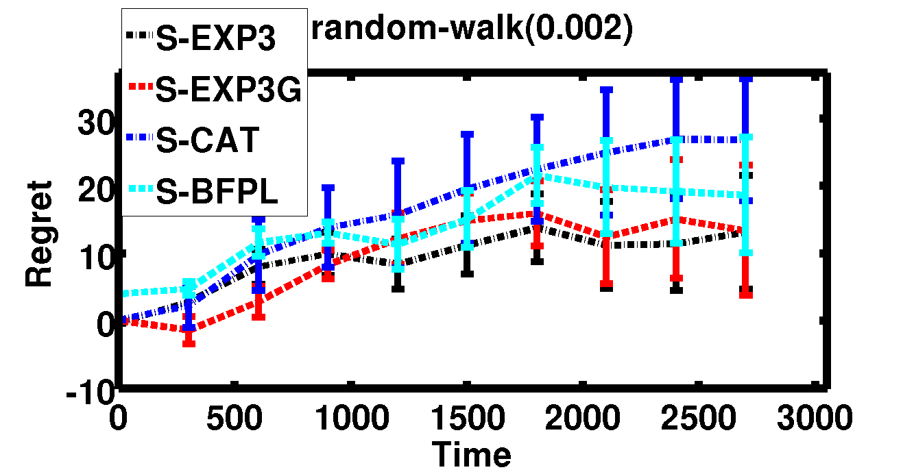
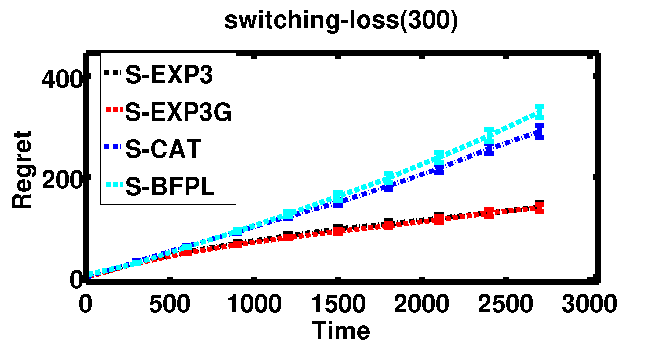
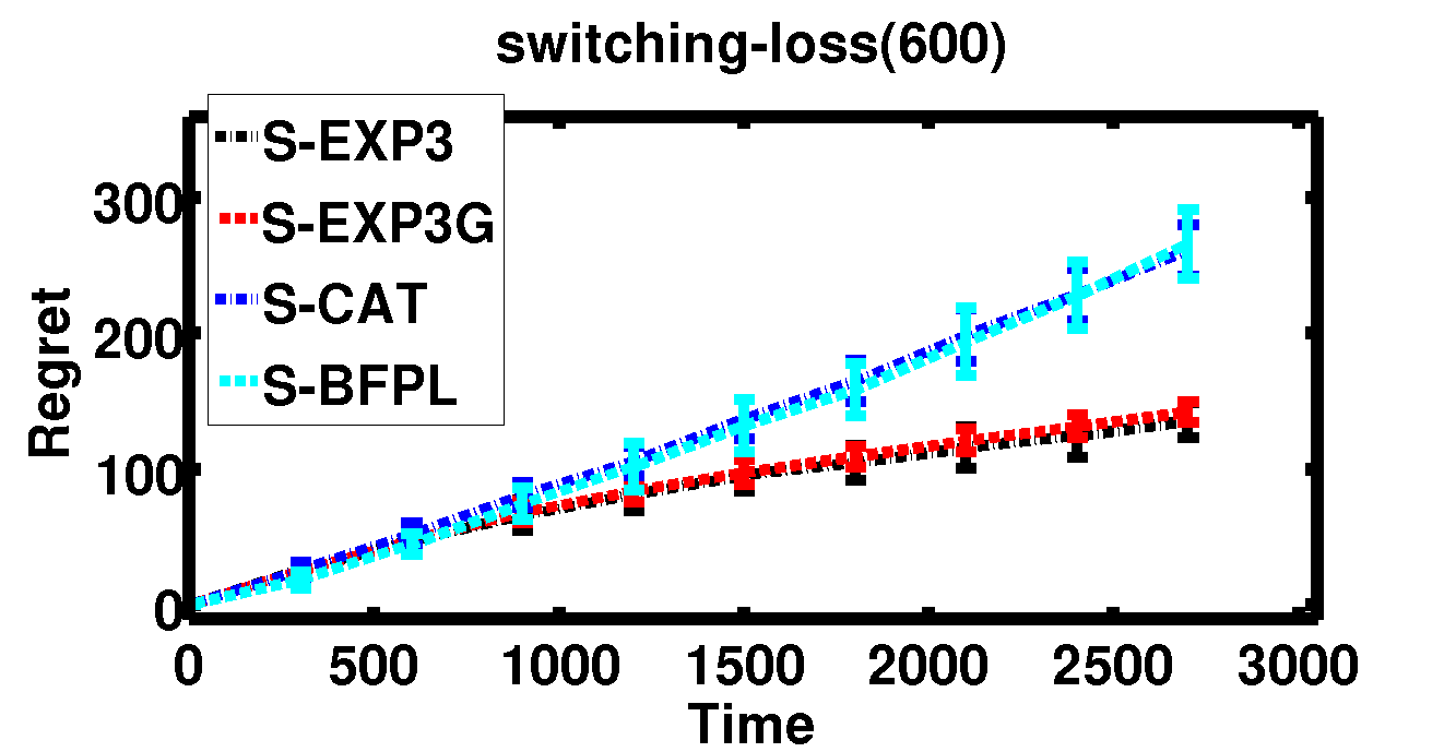
Figure 1: Regret vs Time: Independent availabilities

5 Experiments

In this section we present the empirical evaluation of our proposed algorithms (Sec. 3 and 4) comparing their performances with the two existing sleeping bandit algorithms that apply to our problem setting, i.e. for adversarial losses and stochastic availabilities. Thus we report the comparative performances of the following algorithms:

1. Sleeping-EXP3: Our proposed Alg. 1 (the efficient version as described in Sec. 3.1).

2. Sleeping-EXP3G: Our proposed Alg. 2.

3. Sleeping-Cat: The algorithm proposed by (Neu & Valko, 2014) (precisely their Algorithm for semi-bandit feedback in Sec. $4.3$).

4. Bandit-SFPL: The algorithm proposed by (Kanade et al., 2009) (see Fig. 3, BSFPL algorithm, Sec. $2$).

Performance Measures. In all cases, we report the cumulative regret of the algorithms for $T=5000$ time steps, each averaged over $50$ runs. In the following subsections, we analyze our experimental evaluations for both independent and general (non-independent) availabilities.

5.1 Independent Availabilities

In this case the item availabilities are assumed to be independent at each round (description in Sec. 2).

Environments. We consider $K=20$ and generate the probabilities of item availabilities $\{a_{i}\}_{i\in[K]}$ independently and uniformly at random from the interval $[0.3,0.9]$. We use the following loss generation techniques: $(1)$ Switching loss or SL($\tau$). We generate the loss sequence such that the best performing expert changes after every $\tau$ length epochs. $(2)$ Markov loss or ML(p). Similar to the setting used in (Neu & Valko, 2014), losses for each arm are constructed as random walks with Gaussian increments of standard deviation $p$, initialized uniformly on $[0,1]$ such that losses outside $[0,1]$ are truncated. The explicit values used for $\tau$ and $p$ are specified in the corresponding figures. The algorithm parameters $\eta,\lambda_{t},\delta$ are set as defined in Thm7.

Remarks. From Fig. 1 it clearly shows that regret bounds of our proposed algorithm Sleeping-EXP3  and Sleeping-EXP3G  outperform the other two due to their orderwise optimal $O(\sqrt{T})$ regret performance (see Thm. 2 and 9). In particular, Bandit-SFPL  performs the worst due to its initial $O(T^{4/5})$ exploration rounds and uniform exploration phases thereafter. Sleeping-Cat  gives a much competitive regret bound compared to Bandit-SFPL  however, still lags behind due to the $O(T^{2/3})$ regret guarantee (see Sec. $3.1$ for a detailed explanation).

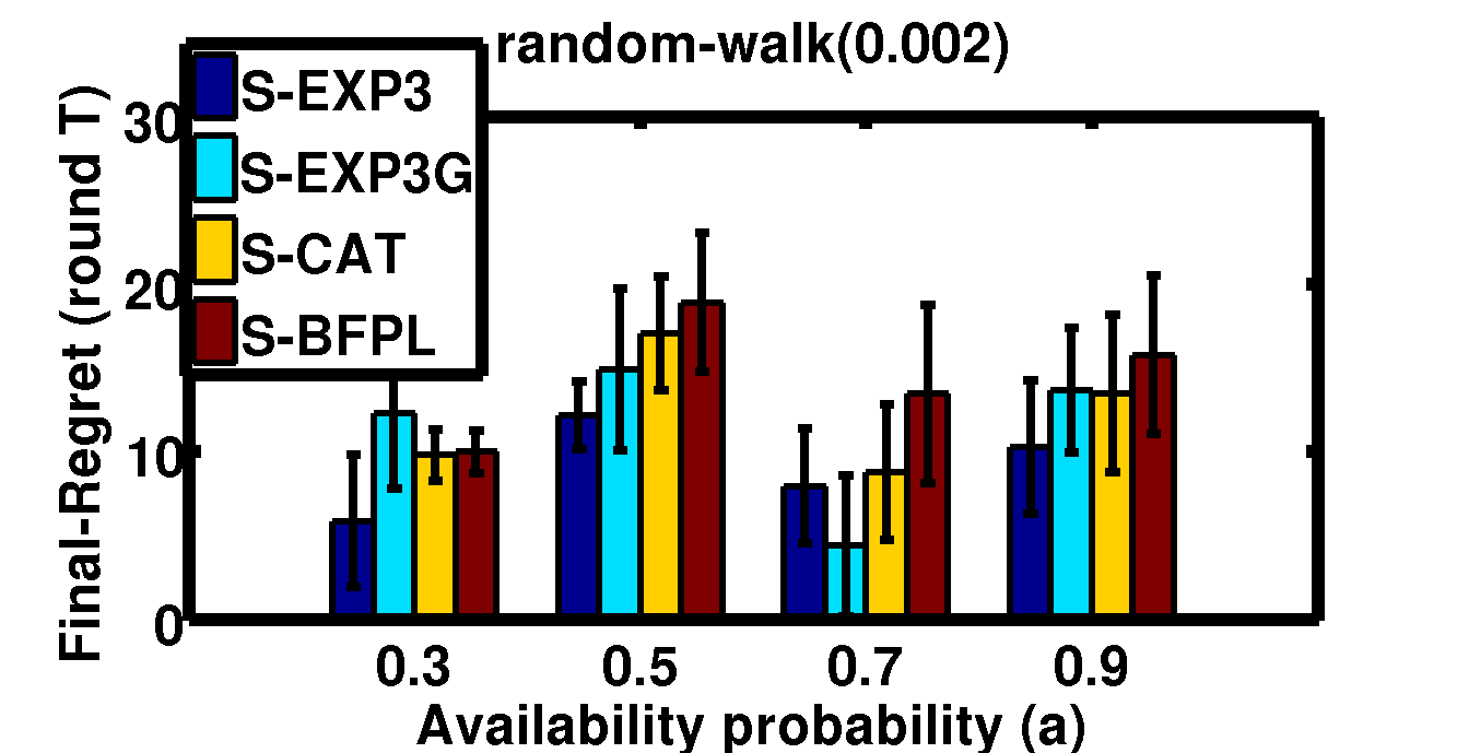
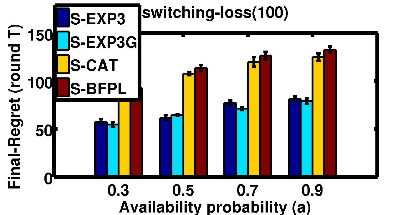
Figure 2: Final regret (at round $T$) vs availability probabilities($(a)$)

5.2 Regret vs Varying Availabilities.

We next conduct a set of experiments to compare the regret performances of the algorithms with varying availability probabilities: For this we assign same availability $a_{i}=a\in[0.1]$ to every item $i\in[K]$ for $a=0.3,0.5,0.7,0.9$ and plot the final cumulative regret of each algorithm.

Remarks From Fig. 2, we again note our algorithms outperform the other two by a large margin for almost every $p$. The performance of BSFPL is worse, it steadily decreases with increasing availability probability due to the explicit $O(T^{4/5})$ exploration rounds in the initial phase of BSFPL, and even thereafter it keeps on suffering the loss of the uniform policy scaled by the exploration probability.

Figure 3: Regret vs time: General availabilities

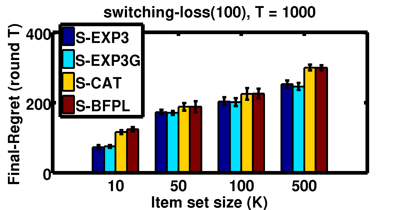
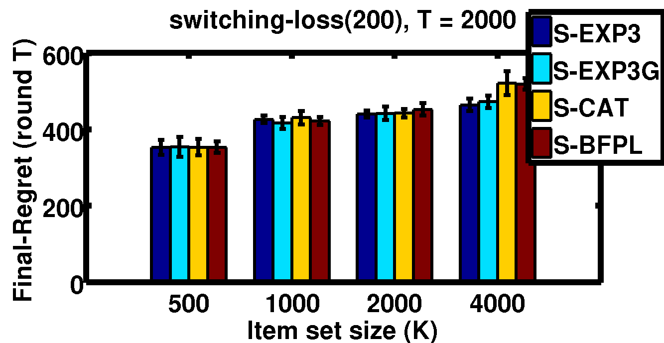
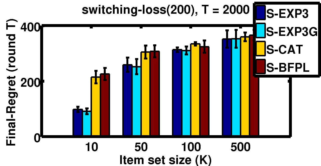
Figure 4: Final regret (at round $T$) vs item size $(K)$

5.3 Correlated (General) Availabilities

We now assess the performances when the availabilities of items are dependent (description in Sec. 2).

Environments. To enforce dependencies of item availabilities we generate each set $S_{t}$ by drawing a random sample from a Gaussian$({\boldsymbol{\mu}},\Sigma)$ such that ${\boldsymbol{\mu}}_{i}=0,\,\forall i\in[K]$, and $\Sigma$ is some random $K\times K$ positive definite matrix, e.g. block diagonal matrix with strong correlations among certain groups of items. More precisely, at each round $t$, we first sample a random $K$-vector, say $v_{t}$, from Gaussian$({\boldsymbol{\mu}},\Sigma)$ and we set $S_{t}={i\in[K]|v_{t}(i)>0}$, i.e. $S_{t}$ includes all those items whose corresponding coordinates are non-negative–this thus enforces item dependencies in the resulted $S_{t}$ if $\Sigma$ is block diagonal (or any correlation matrix). To generate the loss sequences, we use similar techniques described in Sec. 5.1. The algorithm parameters are set as defined in Thm9.

Remarks. From Fig. 3 one can again verify the superior performance of our algorithms over Sleeping-Cat  and Bandit-SFPL, however the effect is only visible for large $T$ as for smaller time steps $t$, the $O(2^{K})$ terms dominates the regret performance, but as $t$ shoots higher our optimal $O(\sqrt{T})$ rate outperforms the suboptimal $O(T^{2/3})$ and $O(T^{4/5})$ rates of Sleeping-Cat  and Bandit-SFPL  respectively.

5.4 Regret vs Varying Item-size $(K)$.

Finally we also conduct a set of experiments changing the item set size $K$ over a wide range ($K=10$ to $4000$). We report the final cumulative regret of all algorithms vs. $K$ for different switching loss sequence for both independent and general availabilities, as specified in Fig. 4.

Remark. Fig. 4 shows that the regret of each algorithm increases with $K$, as expected. As before the other two baselines perform suboptimally in comparison to our algorithms, however the interesting thing to note is the relative performance of Sleeping-EXP3  and Sleeping-EXP3G—as per Thm. 2 and 9, Sleeping-EXP3  must outperform Sleeping-EXP3G  with increasing $K$, however the effect does not seem to be so drastic experimentally, possibly revealing the scope of improving Thm. 9 in terms of a better dependency in $K$.

6 Conclusion and Future Work

We have presented a new approach that brought an improved rate for the setting of sleeping bandits with adversarial losses and stochastic availabilities including both minimax and instance-dependence guarantees. While our bounds guarantee a regret of $\tilde{O}(\sqrt{T}),$ there are several open questions before the studied setting can be considered as closed. Firstly, for the case of independent availabilities, we provide a regret guarantee of $\tilde{O}(K^{2}\sqrt{T})$, leaving open whether $\tilde{O}(\sqrt{KT})$ is possible as in the standard non-sleeping setting. Secondly, while we provided computationally efficient (i.e., with per-round complexity of order $O(tK)$) Sleeping-EXP3, for the case of general availabilities and provided instance dependent regret guarantees for it, the worst case regret guarantee still amounts to $\tilde{O}(\sqrt{2^{K}T}).$ Therefore, it is still unknown if for the general availabilities we can get an algorithm that would be both computationally efficient and have $\tilde{O}(\text{poly}(K)\sqrt{T})$ regret guarantee in the worst case. We would like to point out that the new techniques could be potentially used to provide new algorithms and guarantees in settings with similar challenges as in sleeping bandits, such as rotting or dying bandits. Finally, having algorithms for sleeping bandits with $\tilde{O}(\sqrt{T})$ regret guarantees, opens a way to deal with sleeping constraints in more challenging structured bandits with large or infinite number of arms and having the regret guarantee depend not on number of arms but rather some effective dimension of the arms’ space.

Supplementary: Improved Sleeping Bandits with Stochastic Actions Sets
and Adversarial Rewards

Appendix A Appendix for Sec. 3

A.1 Proof of Lem. 1

See 1

Proof.

Let $t\in[T]$ and $\delta\in(0,1)$. We start by noting the concentration of $\widehat{a}_{ti}=\frac{1}{t}\sum_{\tau=1}^{t}{\mathbf{1}}(i\in S_{\tau})$ to $a_{i}$ for all $i\in[K]$. By Bernstein’s inequality together with a union bound over $i=1,\dots,K$: with probability at least $1-\delta$, for all $i\in[K]$

$$|a_{i}-\widehat{a}_{ti}|<\sqrt{\frac{2a_{i}(1-a_{i})\ln\frac{K}{\delta}}{t}}+\frac{2\ln\frac{K}{\delta}}{3t}\,.$$ (10)

Then, $\beta=2\log(K/\delta)$, using the definitions of $P_{\widehat{\mathbf{a}}_{t}}(S)=\Pi_{i=1}^{K}\widehat{a}_{ti}^{{\mathbf{1}}(i\in S)}(1-\widehat{a}_{ti})^{1-{\mathbf{1}}(i\in S)}$ and $P_{{\mathbf{a}}}(S)=\Pi_{i=1}^{K}a_{i}^{{\mathbf{1}}(i\in S)}(1-a_{i})^{1-{\mathbf{1}}(i\in S)}$, we get

$$|P_{\widehat{\mathbf{a}}_{t}}(S)-P_{{\mathbf{a}}}(S)| =P_{{\mathbf{a}}}(S)\bigg{|}\frac{P_{\widehat{\mathbf{a}}_{t}}(S)}{P_{{\mathbf{a}}}(S)}-1\bigg{|}=P_{{\mathbf{a}}}(S)\bigg{|}\Pi_{i=1}^{K}\bigg{(}\frac{\widehat{a}_{ti}}{a_{i}}\bigg{)}^{S_{i}}\bigg{(}\frac{1-\widehat{a}_{ti}}{1-a_{i}}\bigg{)}^{1-S_{i}}-1\bigg{|}$$

$$=P_{{\mathbf{a}}}(S)\bigg{|}\Pi_{i=1}^{K}\bigg{(}\frac{\widehat{a}_{ti}-a_{i}}{a_{i}}+1\bigg{)}^{S_{i}}\bigg{(}\frac{a_{i}-\widehat{a}_{ti}}{1-a_{i}}+1\bigg{)}^{1-S_{i}}-1\bigg{|}$$

$$\leq P_{{\mathbf{a}}}(S)\bigg{(}\Pi_{i=1}^{K}\bigg{(}\frac{|\widehat{a}_{ti}-a_{i}|}{a_{i}}+1\bigg{)}^{S_{i}}\bigg{(}\frac{|a_{i}-\widehat{a}_{ti}|}{1-a_{i}}+1\bigg{)}^{1-S_{i}}-1\bigg{)}\,,$$ (11)

where the last inequality is because for any $\epsilon_{1},\dots,\epsilon_{K}\in[-1,1]^{K}$

$$\left|\prod_{i=1}^{K}(1+\epsilon_{i})-1\right| =\max\left\{\prod_{i=1}^{K}(1+\epsilon_{i})-1,1-\prod_{i=1}^{K}(1+\epsilon_{i})\right\}$$

$$\leq\max\left\{\prod_{i=1}^{K}\big{(}1+|\epsilon_{i}|\big{)}-1,1-\prod_{i=1}^{K}\big{(}1-|\epsilon_{i}|\big{)}\right\}$$

$$\leq\prod_{i=1}^{K}\big{(}1+|\epsilon_{i}|\big{)}-1\,.$$

Hence, denoting

$$Z_{i}:=\bigg{(}1+\sqrt{\frac{\beta(1-a_{i})}{a_{i}t}}+\frac{\beta}{3a_{i}t}\bigg{)}^{S_{i}}\bigg{(}1+\sqrt{\frac{\beta a_{i}}{(1-a_{i})t}}+\frac{\beta}{3(1-a_{i})t}\bigg{)}^{1-S_{i}}\,,$$

and using Bernstein’s inequality (10), with probability $1-\delta$, we have

$$|P_{\widehat{\mathbf{a}}_{t}}(S)-P_{{\mathbf{a}}}(S)|\leq P_{{\mathbf{a}}}(S)\left(\prod_{i=1}^{K}Z_{i}-1\right)\,.$$ (12)

Therefore,

$$|q^{*}_{t}(i)-\bar{q}_{t}(i)| =\bigg{|}\sum_{S\in 2^{[K]}}q_{t}^{S}(i)\big{(}P_{{\mathbf{a}}}(S)-P_{\widehat{\mathbf{a}}_{t}}(S)\big{)}\bigg{|}\hskip 28.45274pt\leftarrow\text{By definition~{}\eqref{eq:barqt_def}}$$

$$\leq\sum_{S\in 2^{[K]}}q_{t}^{S}(i)\big{|}P_{{\mathbf{a}}}(S)-P_{\widehat{\mathbf{a}}_{t}}(S)\big{|}$$

$$\leq\sum_{S\in 2^{[K]}}P_{{\mathbf{a}}}(S)\left(\prod_{i=1}^{K}Z_{i}-1\right)\hskip 48.36958pt\leftarrow\text{From~{}\eqref{eq:Phat_trueP} and $|q_{t}^{S}(i)|\leq 1$}$$

$$={\mathbf{E}}_{S\sim{\mathbf{P}}_{{\mathbf{a}}}}\left[\prod_{i=1}^{K}Z_{i}\right]-1\,.$$ (13)

But by independence of the $Z_{i}$, we know

$${\mathbf{E}}_{S\sim{\mathbf{P}}_{{\mathbf{a}}}}\left[\prod_{i=1}^{K}Z_{i}\right]=\prod_{i=1}^{K}{\mathbf{E}}_{S\sim{\mathbf{P}}_{{\mathbf{a}}}}\big{[}Z_{i}\big{]}\,.$$ (14)

Now, computing each expectation

$${\mathbf{E}}_{S\sim{\mathbf{P}}_{{\mathbf{a}}}}\big{[}Z_{i}\big{]} ={\mathbf{E}}_{S_{i}\sim a_{i}}\left[\bigg{(}1+\sqrt{\frac{\beta(1-a_{i})}{a_{i}t}}+\frac{\beta}{3a_{i}t}\bigg{)}^{S_{i}}\bigg{(}1+\sqrt{\frac{\beta a_{i}}{(1-a_{i})t}}+\frac{\beta}{3(1-a_{i})t}\bigg{)}^{1-S_{i}}\right]$$

$$=a_{i}\Big{(}1+\sqrt{\frac{\beta(1-a_{i})}{a_{i}t}}+\frac{\beta}{3a_{i}t}\Big{)}+(1-a_{i})\Big{(}1+\sqrt{\frac{\beta a_{i}}{(1-a_{i})t}}+\frac{\beta}{3(1-a_{i})t}\Big{)}$$

$$\leq 1+2\sqrt{\frac{\beta a_{i}(1-a_{i})}{t}}+\frac{2\beta}{3t}$$ (15)

$$\leq 1+\sqrt{\frac{\beta}{t}}+\frac{2\beta}{3t}\,.$$

Therefore, combining with Inequalities (13) and (14), it yields using $1+x\leq e^{x}$ for $x\geq 0$,

$$|q^{*}_{t}(i)-\bar{q}_{t}(i)|\leq\Big{(}1+\sqrt{\frac{\beta}{t}}+\frac{2\beta}{3t}\Big{)}^{K}-1\leq e^{K\sqrt{\frac{\beta}{t}}+\frac{2K\beta}{3t}}-1\,.$$

Then, assuming $t\geq 25\beta K^{2}/9$, we have

$$K\sqrt{\frac{\beta}{t}}+\frac{2K\beta}{3t}\leq 1$$

which implies since $e^{x}\leq 1+2x$ for all $0\leq x\leq 1$ and replacing $\beta=2\log(K/\delta)$

$$|q^{*}_{t}(i)-\bar{q}_{t}(i)|\leq 2K\sqrt{\frac{2\log(K/\delta)}{t}}+\frac{8K\log(K/\delta)}{3t}\,.$$

If $t\leq 15\beta K^{2}/9$, then,

$$|q^{*}_{t}(i)-\bar{q}_{t}(i)|\leq 1\leq\frac{4K}{3}\sqrt{\frac{\log(1/\delta)}{t}}\,.$$

Therefore, for all $\delta\in(0,1)$, with probability at least $1-\delta$, for all $1\leq i\leq K$

$$|q^{*}_{t}(i)-\bar{q}_{t}(i)|\leq 2K\sqrt{\frac{2\log(K/\delta)}{t}}+\frac{8K\log(K/\delta)}{3t}\,.$$

∎

A.2 Proof of Thm. 2

See 2

Proof.

Consider any fixed set $S\subseteq[K]$, and suppose we run EXP3 algorithm on the set $S$, over any nonnegative sequence of losses $\widehat{\ell}_{1},\widehat{\ell}_{2},\ldots\widehat{\ell}_{T}$ over items of set $S$, and consequently with weight updates ${\mathbf{q}}_{1}^{S},{\mathbf{q}}_{2}^{S},\ldots{\mathbf{q}}_{T}^{S}$ where as per EXP3 algorithm

$$q_{t}^{S}(i)=\frac{e^{-\eta\sum_{\tau=1}^{t-1}\widehat{\ell}_{\tau}(i)}}{\sum_{j\in S}e^{-\eta\sum_{\tau=1}^{t-1}\widehat{\ell}_{\tau}(j)}}\,,\quad i\in S$$ (16)

$\eta>0$ being the learning rate of the EXP3 algorithm. Note here that for the analysis, we assume for this hypothetical EXP3 algorithm which plays on actions in $S$ only, the available sets are fixed to $S$ for all $t\in[T]$. We also consider that $q_{t}^{S}(i)=0$ for $i\notin S$.

Then from the standard regret analysis of the EXP3 algorithm it is known that (Cesa-Bianchi & Lugosi, 2006) for all $i\in S$

$$\sum_{t=1}^{T}\big{<}{\mathbf{q}}_{t}^{S},\widehat{\ell}_{t}\big{>}-\sum_{t=1}^{T}\widehat{\ell}_{t}(i)\leq\frac{\log K}{\eta}+\eta\sum_{t=1}^{T}\sum_{k\in S}q_{t}^{S}(k)\widehat{\ell}_{t}(k)^{2}\,.$$

Let $\pi^{*}:S\mapsto[K]$ be any strategy. Then, applying the above regret bound to the choice $i=\pi^{*}(S)$ and taking the expectation over $S\sim P_{{\mathbf{a}}}$ and over the possible randomness of the estimated losses, we get

$$\sum_{t=1}^{T}{\mathbf{E}}\Big{[}\big{<}{\mathbf{q}}_{t}^{S},\widehat{\ell}_{t}\big{>}\Big{]}-\sum_{t=1}^{T}{\mathbf{E}}\Big{[}\widehat{\ell}_{t}(\pi^{*}(S))\Big{]}\leq\frac{\log K}{\eta}+\eta\sum_{t=1}^{T}{\mathbf{E}}\bigg{[}\sum_{k\in S}q_{t}^{S}(k)\widehat{\ell}_{t}(k)^{2}\bigg{]}\,.$$ (17)

Note that we did not make any assumptions on the estimated losses yet expect non-negativity.

For simplicity we abbreviate $S\sim{\mathbf{P}}_{{\mathbf{a}}}$ as $S\sim{\mathbf{a}}$ henceforth. We denote the sigma algebra generated by the history of outcomes till time $t$ (i.e. $\{i_{\tau},S_{\tau}\}_{\tau=1}^{t}$) by ${\mathcal{H}}_{t}$. Then recall from Eqn. (1) that we wish to analyse the regret $R_{T}$, which is defined with respect to the loss sequence $\ell_{1},\ell_{2},\ldots\ell_{T}$ and with activation sets $S_{1},\dots,S_{T}$. That is, we need to upper-bound

$$R_{T}=\max_{\pi:2^{[K]}\mapsto[K]}\left\{\sum_{t=1}^{T}{\mathbf{E}}\big{[}\ell_{t}(i_{t})\big{]}-\sum_{t=1}^{T}{\mathbf{E}}\big{[}\ell_{t}(\pi(S_{t}))\big{]}\right\}\,.$$

Towards proving the above regret bound of Sleeping-EXP3  from Inequality (17), we now first establish the following lemmas that relates the different expectations of Inequality (17) with quantities related to the regret.

See 3

Proof.

Let $t\in[T]$. We first consider the probabilistic event (denoted ${\mathcal{E}}_{t}$) that (5) is true. That is, for all $i\in[K]$

$$|q^{*}_{t}(i)-\bar{q}_{t}(i)|\leq\lambda_{t}\,.$$ (18)

Remark that ${\mathcal{E}}_{t}$ is ${\mathcal{H}}_{t-1}$ measurable since $\bar{\mathbf{q}}_{t}$ and ${\mathbf{q}}_{t}^{*}$ are ${\mathcal{H}}_{t-1}$ measurable.

We start from the right hand side noting that:

$${\mathbf{E}} \Big{[}\big{<}{\mathbf{q}}_{t}^{S},\widehat{\ell}_{t}\big{>}\big{|}{\mathcal{E}}_{t}\Big{]}={\mathbf{E}}\bigg{[}\sum_{i\in S}q_{t}^{S}(i)\widehat{\ell}_{t}(i)\Big{|}{\mathcal{E}}_{t}\bigg{]}$$

$$={\mathbf{E}}\Bigg{[}{\mathbf{E}}\bigg{[}\sum_{i\in S}q_{t}^{S}(i)\dfrac{\ell_{t}(i){\mathbf{1}}(i_{t}=i)}{\bar{q}_{t}(i)+\lambda_{t}}\ \Big{|}\ S,S_{t},{\mathcal{H}}_{t-1}\bigg{]}\bigg{|}\ {\mathcal{E}}_{t}\Bigg{]}\hskip 56.9055pt\leftarrow\text{by definition \eqref{eq:loss_estimate} of $\widehat{\ell}_{t}$}$$

$$={\mathbf{E}}\Bigg{[}{\mathbf{E}}\bigg{[}\sum_{i\in S_{t}}q_{t}^{S}(i)\dfrac{\ell_{t}(i)q_{t}^{S_{t}}(i)}{\bar{q}_{t}(i)+\lambda_{t}}\bigg{|}S_{t},{\mathcal{H}}_{t-1}\bigg{]}\bigg{|}\ {\mathcal{E}}_{t}\Bigg{]}\hskip 82.51282pt\leftarrow\text{taking the expectation over $i_{t}\sim{\mathbf{q}}_{t}^{S_{t}}$}$$

$$={\mathbf{E}}\Bigg{[}{\mathbf{E}}\bigg{[}\sum_{i\in S_{t}}q_{t}^{*}(i)\dfrac{\ell_{t}(i)q_{t}^{S_{t}}(i)}{\bar{q}_{t}(i)+\lambda_{t}}\ \bigg{|}\ {\mathcal{H}}_{t-1}\bigg{]}\bigg{|}{\mathcal{E}}_{t}\Bigg{]}\hskip 93.89418pt\leftarrow\text{taking the expectation over $S\sim{\mathbf{a}}$}$$

$$\geq{\mathbf{E}}\Bigg{[}{\mathbf{E}}\bigg{[}\sum_{i\in S_{t}}q_{t}^{*}(i)\dfrac{\ell_{t}(i)q_{t}^{S_{t}}(i)}{q_{t}^{*}(i)+2\lambda_{t}}\bigg{|}{\mathcal{H}}_{t-1}\bigg{]}\bigg{|}{\mathcal{E}}_{t}\Bigg{]}\hskip 95.3169pt\leftarrow\text{from Inequality~{}\eqref{eq:concentrationqbar}}$$

$$\geq{\mathbf{E}}\Bigg{[}{\mathbf{E}}\bigg{[}\sum_{i\in S_{t}}\ell_{t}(i)q_{t}^{S_{t}}(i)\Big{(}1-\frac{2\lambda_{t}}{q_{t}^{*}(i)}\Big{)}\bigg{|}{\mathcal{H}}_{t-1}\bigg{]}\bigg{|}{\mathcal{E}}_{t}\Bigg{]}\hskip 69.70915pt\leftarrow\text{since $(1+x)^{-1}\geq 1-x$ for $x\geq 0$}$$

$$\geq{\mathbf{E}}\Bigg{[}{\mathbf{E}}\bigg{[}\sum_{i\in S_{t}}\ell_{t}(i)q_{t}^{S_{t}}(i)\bigg{|}{\mathcal{H}}_{t-1}\bigg{]}\bigg{|}{\mathcal{E}}_{t}\Bigg{]}-{\mathbf{E}}\Bigg{[}2\lambda_{t}\sum_{i=1}^{K}\frac{{\mathbf{E}}\big{[}q_{t}^{S_{t}}(i)\big{|}{\mathcal{H}}_{t-1}\big{]}}{q_{t}^{*}(i)}\ \bigg{|}\ {\mathcal{E}}_{t}\Bigg{]}\leftarrow\text{since $q^{*}_{t}$ is ${\mathcal{H}}_{t-1}$ measurable}$$

$$={\mathbf{E}}\bigg{[}{\mathbf{E}}\Big{[}\sum_{i\in S_{t}}\ell_{t}(i)q_{t}^{S_{t}}(i)\Big{|}{\mathcal{H}}_{t-1}\Big{]}\Big{|}\ {\mathcal{E}}_{t}\bigg{]}-2K\lambda_{t}\hskip 28.45274pt\leftarrow\text{by definition of $q^{*}_{t}(i)={\mathbf{E}}\big{[}q_{t}^{S_{t}}(i)\big{|}{\mathcal{H}}_{t-1}\big{]}$}$$

$$={\mathbf{E}}\big{[}\ell_{t}(i_{t})\big{|}{\mathcal{E}}_{t}\big{]}-2K\lambda_{t}\,.$$

It remains now to deal with the case when the event ${\mathcal{E}}_{t}$ (i.e., (18)) is not satisfied. By Lem. 1, this happens with probability smaller than $\delta$. Therefore because the estimated losses are smaller than $1/\lambda_{t}$, we have

$${\mathbf{E}}\Big{[}\big{<}{\mathbf{q}}_{t}^{S},\widehat{\ell}_{t}\big{>}\Big{]} ={\mathbf{E}}\Big{[}\big{<}{\mathbf{q}}_{t}^{S},\widehat{\ell}_{t}\big{>}\ \big{|}\ {\mathcal{E}}_{t}\Big{]}Pr({\mathcal{E}}_{t})+{\mathbf{E}}\Big{[}\big{<}{\mathbf{q}}_{t}^{S},\widehat{\ell}_{t}\big{>}\big{|}\ \text{not }{\mathcal{E}}_{t}\Big{]}Pr\big{(}\text{not }{\mathcal{E}}_{t}\big{)}$$

$$\geq{\mathbf{E}}\big{[}\ell_{t}(i_{t})\big{|}{\mathcal{E}}_{t}]Pr({\mathcal{E}}_{t})-2K\lambda_{t}-\frac{Pr\big{(}\text{not }{\mathcal{E}}\big{)}}{\lambda_{t}}$$

$$\geq{\mathbf{E}}\big{[}\ell_{t}(i_{t})]-2K\lambda_{t}-\frac{\delta}{\lambda_{t}}\,.$$

∎

See 4

Proof.

The proof follows a similar analysis to the one of Lem. 3. We start by assuming the probabilistic event ${\mathcal{E}}_{t}$ of Inequality (18) and to ease the notation, we denote by ${\mathbf{E}}_{t}={\mathbf{E}}\big{[}\ \cdot\ \big{|}{\mathcal{E}}_{t}\big{]}$ the conditional expectation given ${\mathcal{E}}_{t}$ holds true. Then,

$${\mathbf{E}}_{t}\Big{[}\widehat{\ell}_{t}(i)\Big{]} ={\mathbf{E}}_{t}\Bigg{[}{\mathbf{E}}\bigg{[}\dfrac{\ell_{t}(i){\mathbf{1}}(i_{t}=i)}{\bar{q}_{t}(i)+\lambda_{t}}\bigg{|}S_{t},{\mathcal{H}}_{t-1}\bigg{]}\Bigg{]}\hskip 33.28966pt\leftarrow\text{by definition of $\widehat{\ell}_{t}$}$$

$$={\mathbf{E}}_{t}\Bigg{[}{\mathbf{E}}\bigg{[}\dfrac{\ell_{t}(i)q_{t}^{S_{t}}(i)}{\bar{q}_{t}(i)+\lambda_{t}}\bigg{|}{\mathcal{H}}_{t-1}\bigg{]}\Bigg{]}\hskip 59.75095pt\leftarrow\text{taking the expectation over $i_{t}\sim{\mathbf{q}}_{t}^{S_{t}}$}$$

$$={\mathbf{E}}_{t}\Bigg{[}\dfrac{\ell_{t}(i)q_{t}^{*}(i)}{\bar{q}_{t}(i)+\lambda_{t}}\Bigg{]}\hskip 106.41345pt\leftarrow\text{taking the expectation over $S_{t}\sim{\mathbf{a}}$}$$

$$\leq{\mathbf{E}}_{t}\Big{[}\ell_{t}(i)\Big{]}\hskip 133.72786pt\leftarrow\text{by~{}\eqref{eq:concentrationqbar}}$$

$$=\ell_{t}(i)\,.$$

Similarly to the proof of Lem. 3, using that ${\mathcal{E}}$ holds with probability at least $1-\delta$ and using that the estimated losses are in $[0,1/\lambda_{t}]$, we get

$${\mathbf{E}}\Big{[}\widehat{\ell}_{t}(i)\Big{]}\leq\ell_{t}(i)+\frac{\delta}{\lambda_{t}}\,.$$

∎

See 5

Proof.

Let $t\in[T]$. Then, denoting ${\mathcal{E}}_{t}$ the event such that (18) holds, we can derive:

$${\mathbf{E}}_{t}\Bigg{[}\sum_{i\in S}q_{t}^{S}(i)\widehat{\ell}_{t}(i)^{2}\Bigg{]} ={\mathbf{E}}_{t}\Bigg{[}{\mathbf{E}}\bigg{[}\sum_{i\in S}q_{t}^{S}(i)\dfrac{\ell_{t}^{2}(i){\mathbf{1}}(i_{t}=i)}{(\bar{q}_{t}(i)+\lambda_{t})^{2}}\bigg{|}S,S_{t},{\mathcal{H}}_{t-1}\bigg{]}\Bigg{]}\hskip 17.64056pt\leftarrow\text{by definition of $\widehat{\ell}_{t}$}$$

$$={\mathbf{E}}_{t}\Bigg{[}{\mathbf{E}}\bigg{[}\sum_{i\in S_{t}}q_{t}^{S}(i)\dfrac{\ell_{t}^{2}(i)q_{t}^{S_{t}}(i)}{(\bar{q}_{t}(i)+\lambda_{t})^{2}}\bigg{|}S_{t},{\mathcal{H}}_{t-1}\bigg{]}\Bigg{]}\hskip 31.2982pt\leftarrow\text{taking the expectation over $i_{t}\sim{\mathbf{q}}_{t}^{S_{t}}$}$$

$$\leq{\mathbf{E}}\Bigg{[}{\mathbf{E}}\bigg{[}\sum_{i\in S_{t}}q_{t}^{*}(i)\dfrac{q_{t}^{S_{t}}}{(\bar{q}_{t}(i)+\lambda_{t})^{2}}\bigg{|}{\mathcal{H}}_{t-1}\bigg{]}\Bigg{]}\,,$$

where, in the last inequality, we took the expectation over $S_{t}\sim{\mathbf{a}}$ and used that $\ell_{t}(i)^{2}\leq 1$. Therefore, taking the expectation over $S_{t}\sim{\mathbf{a}}$, we get

$${\mathbf{E}}_{t}\Bigg{[}\sum_{i\in S}q_{t}^{S}(i)\widehat{\ell}_{t}(i)^{2}\Bigg{]} \leq{\mathbf{E}}_{t}\Bigg{[}\sum_{i\in[K]}\dfrac{q_{t}^{*}(i)^{2}}{(\bar{q}_{t}(i)+\lambda_{t})^{2}}\Bigg{]}\leq K\,,$$

where the last inequality is because under ${\mathcal{E}}_{t}$, $|\bar{q}_{t}(i)-q_{t}^{*}(i)|\leq\lambda_{t}$. Now, using that $\widehat{\ell}_{t}(i)^{2}\leq 1/\lambda_{t}^{2}$, and using that ${\mathcal{E}}_{t}$ is satisfied with probability at least $1-\delta$, we conclude the proof of the lemma:

$${\mathbf{E}}\Bigg{[}\sum_{i\in S}q_{t}^{S}(i)\widehat{\ell}_{t}(i)^{2}\Bigg{]}\leq K+\frac{\delta}{\lambda_{t}^{2}}\,.$$

∎

Given the above claims in place, we are now in a position to prove the main theorem as shown below. Recall from Eqn. (1), the actual regret definition of our proposed algorithm:

$$R_{T}(\text{{\it Sleeping-EXP3}})=\max_{\pi:2^{[K]}\mapsto[K]}\sum_{t=1}^{T}{\mathbf{E}}\Big{[}\ell_{t}(i_{t})-\ell_{t}(\pi(S_{t}))\Big{]}$$

Denoting the best policy $\pi^{*}:=\arg\min_{\pi:2^{[K]}\mapsto[K]}\sum_{t=1}^{T}{\mathbf{E}}_{S_{t}\sim P_{{\mathbf{a}}}}[\ell(\pi(S_{t}))]$, and combining the claims from Lem. 3, 4, we get:

$$R_{T} (\text{{\it Sleeping-EXP3}})=\sum_{t=1}^{T}{\mathbf{E}}\Big{[}\ell_{t}(i_{t})-\ell_{t}(\pi^{*}(S_{t}))\Big{]}$$

$$\leq\sum_{t=1}^{T}{\mathbf{E}}\Big{[}\big{<}{\mathbf{q}}_{t}^{S},\widehat{\ell}_{t}\big{>}+2K\lambda_{t}+\frac{\delta}{\lambda_{t}}-\widehat{\ell}_{t}(\pi^{*}(S_{t}))+\frac{\delta}{\lambda_{t}}\Big{]}\hskip 28.45274pt\leftarrow\text{from Lemmas~{}\ref{lem:first_term} and~{}\ref{lem:second_term}}$$

$$\leq 2K\sum_{t=1}^{T}\lambda_{t}+2\sum_{t=1}^{T}\frac{\delta}{\lambda_{t}}+\sum_{t=1}^{T}{\mathbf{E}}\Big{[}\big{<}{\mathbf{q}}_{t}^{S},\widehat{\ell}_{t}\big{>}-\widehat{\ell}_{t}(\pi^{*}(S))\Big{]}\,.$$

Then, we can further upper-bound the last term in the right-hand-side using Inequality (17) and Lem. 5, which yields

$$R_{T}(\text{{\it Sleeping-EXP3}}) \leq 2K\sum_{t=1}^{T}\lambda_{t}+2\sum_{t=1}^{T}\frac{\delta}{\lambda_{t}}+\frac{\log K}{\eta}+\eta\sum_{t=1}^{T}{\mathbf{E}}\bigg{[}\sum_{k\in S}q_{t}^{S}(k)\widehat{\ell}_{t}(k)^{2}\bigg{]}$$

$$\leq 2K\sum_{t=1}^{T}\lambda_{t}+2\sum_{t=1}^{T}\frac{\delta}{\lambda_{t}}+\frac{\log K}{\eta}+\eta KT+\eta\sum_{t=1}^{T}\frac{\delta}{\lambda_{t}^{2}}$$

$$\leq\frac{\log K}{\eta}+\eta KT+2K\sum_{t=1}^{T}\lambda_{t}+3\sum_{t=1}^{T}\frac{\delta}{\lambda_{t}^{2}}\,,$$ (19)

where in the last-inequality we used that $\eta\leq 1$ and $\lambda_{t}\leq 1$. Otherwise, we can always choose $\min\{1,\lambda_{t}\}$ instead of $\lambda_{t}$ in the algorithm and Lem. 1 would still be satisfied.

The proof is concluded by replacing $\lambda_{t}=2K\sqrt{\frac{2\log(K/\delta)}{t}}+\frac{8K\log(K/\delta)}{3t}$ and by upper-bounding the two sums

$$\sum_{t=1}^{T}\lambda_{t} =2K\sqrt{2\log\Big{(}\frac{K}{\delta}\Big{)}}\sum_{t=1}^{T}\frac{1}{\sqrt{t}}+\frac{8K}{3}\log\Big{(}\frac{K}{\delta}\Big{)}\sum_{t=1}^{T}\frac{1}{t}$$

$$\leq 2K\sqrt{2\log\Big{(}\frac{K}{\delta}\Big{)}T}+\frac{8K}{3}\log\Big{(}\frac{K}{\delta}\Big{)}(1+\log T)$$

and using $\lambda_{t}\geq 2K\sqrt{2\log(K/\delta)/t}$, we have

$$\sum_{t=1}^{T}\frac{1}{\lambda_{t}^{2}} \leq\frac{1}{8K^{2}\log(K/\delta)}\sum_{t=1}^{T}t\leq\frac{T^{2}}{8K^{2}\log(K/\delta)}\leq\frac{T^{2}}{8K^{2}}\,.$$

Then, using $\delta:=K/T^{2}$, $\log(K/\delta)=2\log(T)$, we can further upper-bound:

$$\sum_{t=1}^{T}\lambda_{t}\leq 4K\sqrt{T\log T}+\frac{8K}{3}(1+\log T)(\log T)\leq 7K\sqrt{T\log T}$$

and

$$3\sum_{t=1}^{T}\frac{\delta}{\lambda_{t}^{2}}\leq\frac{3}{8K}\leq 1\,.$$

Thus, upper-bounding the two sums into (19), we get

$$R_{T}(\text{{\it Sleeping-EXP3}})\leq\frac{\log K}{\eta}+\eta KT+14K^{2}\sqrt{T\log T}+1\,.$$

Optimizing $\eta=\sqrt{(\log K)/KT}$ and upper-bounding $\sqrt{KT\log K}\leq K^{2}\sqrt{T}$, we finally conclude the proof

$$R_{T}(\text{{\it Sleeping-EXP3}})\leq 16K^{2}\sqrt{T\log T}+1\,.$$

∎

A.3 Proof of Lem. 6

See 6

Proof.

Let $t\in[T]$. We start by remarking that for any $i\in[K]$:

$$|q^{*}_{t}(i)-\tilde{q}_{t}(i)|\leq|q^{*}_{t}(i)-\bar{q}_{t}(i)|+|\bar{q}_{t}(i)-\tilde{q}_{t}(i)|\,.$$ (20)

Note that ${\mathbf{q}}_{t}^{S^{(1)}_{t}}(i),{\mathbf{q}}_{t}^{S^{(2)}_{t}}(i),\ldots{\mathbf{q}}_{t}^{S^{(T)}_{t}}(i)$ are independent of each other given the past ${\mathcal{H}}_{t-1}$. Furthermore, they are in $[0,1]$ and are unbiased estimates of $\bar{q}_{t}(i)={\mathbf{E}}_{S\sim\widehat{\mathbf{a}}_{t}}[q_{t}^{S}(i)]$, i.e., for all $i\in[K],\tau\in[t]$

$${\mathbf{E}}_{\widehat{\mathbf{a}}_{t}}\Big{[}{\mathbf{q}}_{t}^{S^{(\tau)}_{t}}(i)\Big{]}=\bar{\mathbf{q}}_{t}(i)\,.$$

Thus, using Hoeffding’s inequality and a union bound over all $i\in[K]$, we get that with probability at least $(1-\delta/2)$:

$$|\bar{q}_{t}(i)-\tilde{q}_{t}(i)|\leq\sqrt{\frac{1}{2t}\ln\frac{2K}{\delta}}\,.$$ (21)

Furthermore, from Lem. 1 we have, for all $i\in[K]$, with probability at least $(1-\delta/2)$:

$$|q^{*}_{t}(i)-\bar{q}_{t}(i)|\leq 2K\sqrt{\frac{2\log(2K/\delta)}{t}}+\frac{8K\log(2K/\delta)}{3t}.$$ (22)

The proof follows combining Eqn. (20), (21) and (22) and using $K\geq 1$. ∎

A.4 Proof of Thm. 7

See 7

Proof.

The regret bound can be proved using the same proof technique used for Thm. 2, except replacing the concentration result of Lem. 6 in place of Lem. 1.

Concerning the computational time. At each round $t\geq 1$, the Alg. 1 performs the following operations:

• update $\widehat{a}_{ti}$ for all $i\in[K]$                                                                                            $\rightarrow$ Cost $O(K)$

• for each $\tau\in[t]$, sample $S_{t}^{(\tau)}$ from $P_{\widehat{\mathbf{a}}_{t}}$ and compute ${\mathbf{q}}_{t}^{S_{t}^{(\tau)}}(i)\propto p_{t}(i){\mathbf{1}}\big{(}i\in S_{t}^{(\tau)}\big{)}$ for each $i\in[K]$    $\rightarrow$ Cost $O(tK)$

• compute the estimated losses $\widehat{\ell}_{t}(i)$ and update $p_{t+1}(i)$ for each $i\in[K]$                                     $\rightarrow$ Cost $O(K)$

The time complexity to perform iteration $t$ is therefore $O(tK)$.

As for spatial complexity, the algorithm only needs to keep track of $\widehat{\mathbf{a}}_{t}\in[0,1]^{K}$ and ${\mathbf{p}}_{t}\in[0,1]^{K}$. Since the step b) above can also be performed sequentially, the total storage complexity is $O(K)$. ∎

Appendix B Appendix for Sec. 4

See 8

Proof.

Let $t\in[T]$. We start by first noting the concentration of $\widehat{P}(S)$ for any $S\subseteq[K]$, which using Bernstein’s inequality we know that given any fixed $\delta\in[0,1]$:

$$Pr\bigg{(}|P(S)-\widehat{P}_{t}(S)|>\sqrt{\frac{2P(S)(1-P(S))\ln\frac{1}{\delta}}{t}}+\frac{2\ln\frac{1}{\delta}}{3t}\bigg{)}\leq\delta\,.$$

Then consider the event

$${\mathcal{E}}_{t}:=\left\{\forall S\subseteq[K]:|P(S)-\widehat{P}_{t}(S)|>\sqrt{\frac{2P(S)(1-P(S))\ln\frac{2^{K}}{\delta}}{t}}+\frac{2\ln\frac{2^{K}}{\delta}}{3t}\right\}\,.$$ (23)

Taking a union bound over all $2^{K}$ subsets $S\subseteq[K]$, we get that: $Pr({\mathcal{E}}_{t})\geq 1-\delta$. Now recall in this case that by definition

$$q^{*}_{t}(i):={\mathbf{E}}_{S\sim{\mathbf{P}}}[q_{t}^{S}(i)]=\sum_{S\in 2^{[K]}}P(S)q_{t}^{S}(i),$$ (24)

and similarly,

$$\bar{q}_{t}(i):=\frac{1}{t}\sum_{\tau=1}^{t}q_{t}^{S_{\tau}}(i)={\mathbf{E}}_{S\sim\widehat{P}_{t}(S)}[q_{t}^{S}(i)]=\sum_{S\in 2^{[K]}}\widehat{P}_{t}(S)q_{t}^{S}(i),$$ (25)

with $\widehat{P}_{t}(S):=\frac{1}{t}\sum_{\tau=1}^{t}{\mathbf{1}}(S_{\tau}=S)$. To ease the notation, let us denote $S_{i}={\mathbf{1}}(i\in S)$.

We now proceed to bound $|q_{t}^{*}(i)-\bar{q}_{t}(i)|$ for any item $i\in[K],\,t\in[T]$. Let us denote $Q_{t}(i)=\sum_{S\in 2^{[K]}}q_{t}^{S}(i)$. Note that $Q_{t}(i)\leq 2^{K}$. Let us also define for simplicity $\alpha(S)=2P(S)(1-P(S))\ln(2^{K}/\delta)$ and $\beta=\frac{2}{3}\ln(2^{K}/\delta)$ the terms in the right-hand-side of (23). Then, following the above claims we note that from (23) with probability at least $(1-\delta)$,

$$|q^{*}_{t}(i)-\bar{q}_{t}(i)| \leq\sum_{S\in 2^{[K]}}q_{t}^{S}(i)\big{|}P(S)-\widehat{P}_{t}(S)\big{|}\hskip 56.9055pt\leftarrow\text{from \eqref{eq:qstar_sum} and~{}\eqref{eq:qbar_sum}}$$

$$\leq\sum_{S\in 2^{[K]}}q_{t}^{S}(i)\bigg{(}\sqrt{\frac{\alpha(S)}{t}}+\frac{\beta}{t}\bigg{)}\hskip 54.06006pt\leftarrow\text{from \eqref{eq:event_general}}$$

$$\leq\frac{\beta 2^{K}}{t}+Q_{t}(i)\sum_{S\in 2^{[K]}}\frac{q_{t}^{S}(i)}{Q_{t}(i)}\sqrt{\frac{\alpha(S)}{t}}\hskip 28.45274pt\leftarrow\text{because $Q_{t}(i)\leq 2^{K}$}$$

$$\leq\frac{\beta 2^{K}}{t}+Q_{t}(i)\sqrt{\sum_{S\in 2^{[K]}}\frac{q_{t}^{S}(i)\alpha(S)}{Q_{t}(i)t}}\hskip 34.14322pt\leftarrow\text{from Jensen's inequality}$$

$$\leq\sqrt{\frac{2^{K+1}}{t}\ln\frac{2^{K}}{\delta}}+\frac{2^{K+1}}{3t}\ln\frac{2^{K}}{\delta},$$

where the last inequality is because $Q_{t}(i)\leq 2^{K}$ and

$$\sum_{S\in 2^{[K]}}q_{t}^{S}(i)\alpha(S)\leq\sum_{S\in 2^{[K]}}\alpha(S)\leq 2\log(2^{K}/\delta)\sum_{S\in 2^{[K]}}P(S)\leq 2\log(2^{K}/\delta)\,.$$

This concludes the proof of the Lemma. ∎

B.1 Proof of Thm. 9

See 9

Proof.

The proof is almost similar to the proof of Thm. 2. We use the same notation introduced in that proof for ease of understanding. Same as before the proof relies on the Lemmas 3, 4, and 5 that are satisfied but for

$$\lambda_{t}=\sqrt{\frac{2^{K+1}}{t}\ln\frac{2^{K}}{\delta}}+\frac{2^{K+1}}{3t}\ln\frac{2^{K}}{\delta}\,,$$

since we need to use the concentration Lem. 8 instead of Lem. 1. Now, recall from Eqn. (1), the actual regret definition of our proposed algorithm:

$$R_{T}(\text{{\it Sleeping-EXP3G}})=\max_{\pi:2^{[K]}\mapsto[K]}\sum_{t=1}^{T}{\mathbf{E}}\Big{[}\ell_{t}(i_{t})-\ell_{t}(\pi(S_{t}))\Big{]}$$

Denoting the best policy $\pi^{*}:=\arg\min_{\pi:2^{[K]}\mapsto[K]}\sum_{t=1}^{T}{\mathbf{E}}_{S_{t}\sim P_{{\mathbf{a}}}}[\ell(\pi(S_{t}))]$, and combining the claims from Lem. 3, 4 and 5, we get following the same arguments as the ones of Thm. 2:

$$R_{T} (\text{{\it Sleeping-EXP3G}})=\sum_{t=1}^{T}{\mathbf{E}}\Big{[}\ell_{t}(i_{t})-\ell_{t}(\pi^{*}(S_{t}))\Big{]}$$

$$\leq\sum_{t=1}^{T}{\mathbf{E}}\big{[}\big{<}{\mathbf{q}}_{t}^{S},\widehat{\ell}_{t}\big{>}+2K\lambda_{t}+\frac{2\delta}{\lambda_{t}}\big{]}-{\mathbf{E}}[\widehat{\ell}_{t}(\pi^{*}(S_{t}))]\hskip 68.28644pt\leftarrow\text{from Lem.~{}\ref{lem:first_term} and Lem.~{}\ref{lem:second_term}}$$

$$=\sum_{t=1}^{T}{\mathbf{E}}\Big{[}\big{<}{\mathbf{q}}_{t}^{S},\widehat{\ell}_{t}\big{>}-\widehat{\ell}_{t}(\pi^{*}(S))\Big{]}+2\sum_{t=1}^{T}\big{(}K\lambda_{t}+\frac{\delta}{\lambda_{t}}\big{)}$$

$$\leq\frac{\log K}{\eta}+\eta\sum_{t=1}^{T}{\mathbf{E}}\bigg{[}\sum_{k\in S}q_{t}^{S}(k)\widehat{\ell}_{t}(k)^{2}\bigg{]}+2\sum_{t=1}^{T}\big{(}K\lambda_{t}+\frac{\delta}{\lambda_{t}}\big{)}\hskip 28.45274pt\leftarrow\text{from Inequality~{}\eqref{eq:RegretEXP3}}$$

$$\leq\frac{\log K}{\eta}+\eta KT+\sum_{t=1}^{T}\big{(}2K\lambda_{t}+\frac{2\delta}{\lambda_{t}}+\frac{\eta\delta}{\lambda_{t}^{2}}\big{)}\hskip 91.04872pt\leftarrow\text{from Lem.~{}\ref{lem:var_term}}$$

$$\leq\frac{\log K}{\eta}+\eta KT+\sum_{t=1}^{T}\big{(}2K\lambda_{t}+\frac{3\delta}{\lambda_{t}^{2}}\big{)}\hskip 116.65646pt\leftarrow\text{because $\eta\leq 1$ and $\lambda_{t}\leq 1$}$$

To conclude the proof, it only remains to compute the sums and to choose the parameters $\delta=2^{K}/T^{2}$ and $\eta=\sqrt{(\log K)/KT}$. Using $\lambda_{t}\geq\sqrt{2^{K+1}/t}$, we have

$$\sum_{t=1}^{T}\frac{\delta}{\lambda_{t}^{2}}\leq\frac{\delta T^{2}}{2^{K+1}}\leq 1$$

and since $\log(2^{K}/\delta)=2\log T$,

$$\lambda_{t}=\sqrt{\frac{2^{K+1}}{t}\ln T}+\frac{2^{K+1}}{3t}\ln T$$

which entails

$$\sum_{t=1}^{T}\lambda_{t}\leq\sqrt{2^{K+1}T\log T}+\frac{2^{K+1}}{3}(\log T)(1+\log T)\leq\sqrt{2^{K+1}T\log T}+2^{K+2}(\log T)^{2}\,.$$

Substituting $\eta$ and these upper-bounds in the regret upper-bound concludes the proof:

$$R_{T}(\text{{\it Sleeping-EXP3G}}) \leq 2\sqrt{KT\log K}+K\sqrt{2^{K+3}T\log T}+K2^{K+3}(\log T)^{2}$$

$$\leq K\sqrt{2^{K+4}T\log T}+K2^{K+3}(\log T)^{2}\,.$$

As for the complexity, the only difference with Alg. 1 comes from the computation of $\bar{q}_{t}(i)$. The latter can also be performed with a computational cost of $O(tK)$. Yet, the algorithm needs to keep in memory the empirical distribution of $S_{1},\dots,S_{t}$. Thus, a space complexity of $O(K+\min\{tK,2^{K}\})$. ∎

References

• Agrawal & Goyal (2012) Agrawal, S. and Goyal, N. Analysis of thompson sampling for the multi-armed bandit problem. In Conference on Learning Theory, pp.  39–1, 2012.
• Auer (2000) Auer, P. Using upper confidence bounds for online learning. In Foundations of Computer Science, 2000. Proceedings. 41st Annual Symposium on, pp.  270–279. IEEE, 2000.
• Auer (2002) Auer, P. Using confidence bounds for exploitation-exploration trade-offs. Journal of Machine Learning Research, 3(Nov):397–422, 2002.
• Auer et al. (2002a) Auer, P., Cesa-Bianchi, N., and Fischer, P. Finite-time analysis of the multiarmed bandit problem. Machine learning, 47(2-3):235–256, 2002a.
• Auer et al. (2002b) Auer, P., Cesa-Bianchi, N., Freund, Y., and Schapire, R. E. The nonstochastic multiarmed bandit problem. SIAM journal on computing, 32(1):48–77, 2002b.
• Bubeck et al. (2012) Bubeck, S., Cesa-Bianchi, N., et al. Regret analysis of stochastic and nonstochastic multi-armed bandit problems. Foundations and Trends® in Machine Learning, 5(1):1–122, 2012.
• Cesa-Bianchi & Lugosi (2006) Cesa-Bianchi, N. and Lugosi, G. Prediction, learning, and games. Cambridge university press, 2006.
• Cortes et al. (2019) Cortes, C., Desalvo, G., Gentile, C., Mohri, M., and Yang, S. Online learning with sleeping experts and feedback graphs. In International Conference on Machine Learning, pp. 1370–1378, 2019.
• Even-Dar et al. (2006) Even-Dar, E., Mannor, S., and Mansour, Y. Action elimination and stopping conditions for the multi-armed bandit and reinforcement learning problems. Journal of machine learning research, 7(Jun):1079–1105, 2006.
• Kale et al. (2016) Kale, S., Lee, C., and Pál, D. Hardness of online sleeping combinatorial optimization problems. In Advances in Neural Information Processing Systems, pp. 2181–2189, 2016.
• Kanade & Steinke (2014) Kanade, V. and Steinke, T. Learning hurdles for sleeping experts. ACM Transactions on Computation Theory (TOCT), 6(3):11, 2014.
• Kanade et al. (2009) Kanade, V., McMahan, H. B., and Bryan, B. Sleeping experts and bandits with stochastic action availability and adversarial rewards. 2009.
• Kleinberg et al. (2010) Kleinberg, R., Niculescu-Mizil, A., and Sharma, Y. Regret bounds for sleeping experts and bandits. Machine learning, 80(2-3):245–272, 2010.
• Neu & Valko (2014) Neu, G. and Valko, M. Online combinatorial optimization with stochastic decision sets and adversarial losses. In Advances in Neural Information Processing Systems, pp. 2780–2788, 2014.
• Vermorel & Mohri (2005) Vermorel, J. and Mohri, M. Multi-armed bandit algorithms and empirical evaluation. In European conference on machine learning, pp.  437–448. Springer, 2005.