Long range alternating spin current order in a quantum wire with modulated spin-orbit interactions

Abstract

A key concept in the emerging field of spintronics is the electric field control of spin precession via the effective magnetic field generated by the Rashba spin orbit interaction (RSOI). Here, by extensive Density Matrix Renormalization Group computations, we demonstrate the presence of alternating spin current order in the gapped phases of a quantum wire with spatially modulated RSOI and repulsive electron-electron interactions. Our results are analytically supported by bosonization and by a mapping to a locally rotated spin basis.

I Introduction

The possibility to manipulate magnetization at nanoscale using the coupling between the electron spin and its motion (orbital angular momentum) has led to the emergence of a new research field named ”spin-orbitronics” [Wolf_et_al_Science_01, ; Fabian_Zutic_Review_04, ; Fabian_Zutic_Review_09, ; Awschalom_etal_13, ]. The main advantage of this approach is based on the exploitation of the spin-orbit (SO) interaction [Winkler_Book_03, ] to get efficient ways for manipulating the magnetization in integrated spintronic systems and create a low power storage and/or logic devices [Awschalom_etal_02, ; Morton_etal_11, ]. The seminal proposal of Datta and Das for a spin field-effect transistor highlights the use of the SO interaction [Datta_Das_90, ]. A basic ingredient of the Datta-Das transistor is a ballistic quantum wire with sufficiently strong Rashba spin-orbit interaction (RSOI) [Rashba_60, ], the latter is required for creating a sizeable spin precession. Depending on spin orientations in the source and in the drain one can modulate the current flowing through the device and thus implement in principle ON/OFF states. The strength of the spin-orbit coupling can be tuned by applying a gate voltage to the system [DD_Transistor_1, ; DD_Transistor_2, ]. In two dimensional structures, coupling between the charge and spin degrees of freedom via the SO interaction provides a mechanism for efficient conversions between charge and spin currents. The spin Hall effect [Dyakonov_Perel_71, ; HE_Sinova_etal_RMP_15, ] by which a charge current can be converted into a transverse spin current and the inverse spin Hall effect [Inv_HE_1, ; Inv_HE_2, ] for the inverse conversion are the primary examples.

In last years the SO effects in quasi-one-dimensional strongly correlated electron systems have became the subject of intensive studies due to their fascinating properties and wide possibilities to engineer new materials with unconventional electronic and magnetic properties. This includes helical conductors which appear in the presence of strong spin-orbit interaction in quantum wires [Streda_03, ], nanotubes [Klinovaja_etal_11, ] or on the edges of topological insulators [Hasan_Kane_RMP_2010, ]. Helical conductors have became of topical interest because their robustness with respect to the disorder [SJJ_10, ] and because they offer the possibility for spin-filtered transport [Streda_03, ; Cabra_etal_17, ], Cooper pair splitting [Sato_etal_10, ] and, if in contact with a superconductor, the realization of Majorana bound states at their ends [Alicea_12, ; Fu_Kane_08, ; Lutchyn_etal_10, ; Oreg_etal_10, ; Alicea_etal_1l, ; Yazdani_etal_13, ; MJJ_Paper_16, ].

Another fascinating property of the SO interaction is that it can be exploited to engineer magnetic materials in which new types of topological objects, such as chiral domain walls or magnetic skyrmions can be stabilized (see for recent review [Balents_Savary_17, ; Legrand_etal_18, ]). Such spin configurations are driven by an additional term in the exchange interaction, namely Dzyaloshinskii-Moriya interaction (DMI) [Dzyaloshinskii_57, ], which arises from the presence of SO coupling and inversion symmetry breaking [Moriya_60, ]. In quasi-one-dimensional magnetic materials the DMI is responsible for formation of a chiral order [Dzyaloshinskii_64, ; Oshikawa_Affleck, ; Aristov_Maleev_00, ; Tsvelick_01, ; Starykh_08, ; Garate_Affleck_10, ; Starykh_17, ]. It is also the key structural element ensuring coupling between magnetic and electric degrees of freedom in the spin-driven chiral multiferroic materials [Katsura_05, ; Ch-MFS, ]. These systems became very actual in last years [SD-Ch-MFM, ], in particular in the context of materials useful for electric field controlled quantum information processing.

Recently it has been demonstrated that the SO interaction can be tailored with a substantial efficiency factor by external electric fields as in a metallic phase of a quantum wire [EF_Enhanc_SOI, ], as well as in the case of insulating quantum magnet [EF_Enhanc_DMI, ]. This unveils the possibility to control SO interaction and magnetic anisotropy via the electric field and opens a wide area for exploring the effects caused by the spatially modulated SO interaction on the properties of low-dimensional electron systems both in conducting and insulating phases.

Theoretical studies of the one-dimensional correlated electron systems with spatially modulated SO interactions of different genesis, counts almost two decades [Cabra_etal_17, ,Mireles_Kirczenow_01, ; Wang_04, ; GongYang_07, ; Zhang_etal_05, ; Wang_etal_06, ; Sanchez_Serra, ; JJF_09, ; Xiao_Chen_10, ; MGJJ_11, ; JJM_14, ; MJJ_Paper_16, ; AJR_19, ]. A Peierls-type mechanism for a spin-based current switch was identified in [JJF_09, ], where it was shown that a spatially smooth modulated Rashba SOI coupling opens both charge and spin gaps in the system at commensurate band fillings. Such an interaction could be generated by a periodic gate configuration, as sketched in [Cabra_etal_17, ], or in contact with an anti-ferroelectrically ordered material [Streltsov-20015, ]. In subsequent studies the effect of induced charge density wave correlations in the quantum wire due to the periodic potential was examined, and the optimal regime where insulating current blockade occurs was determined [MGJJ_11, ]. Later it was shown that the half-metal phase, where electrons with only a selected spin polarization exhibit ballistic conductance, can be reached by tuning of a uniform external magnetic field acting on a quantum wire with modulated spin-orbit interaction [Cabra_etal_17, ]. More recently it was shown that, in the case of a half-filled band and in the limit of strong Coulomb repulsion where the charge excitations are gapped and the spin degrees of freedom are described by an effective spin $S=1/2$ Heisenberg chain, the very presence of spatially modulated DMI substantially enriches the ground state phase diagram of the spin system leading to the formation of a new gapped phases with composite order characterized by the coexisting of bond-located alternating dimerization and chirality patterns and, for a particular parameter range, also of the staggered on-site magnetization [AJR_19, ].

In the present article we put forward studies of the insulating phases of one-dimensional electron systems with modulated Rashba spin-orbit interaction including, in one scheme, analysis of the band-filling commensurability conditions necessary for the formation of band insulating phases [JJF_09, ] together with consideration of the effects caused by the strong electron-electron interaction, responsible for the formation of a Mott correlated insulator phase effectively described by the above mentioned spin chain Hamiltonian [AJR_19, ]. We present a detailed study of the excitation spectrum, as well as alternating charge and spin order in the ground state of a one-dimensional system of electrons with spatially modulated RSOI, mainly using Density Matrix Renormalization Group (DMRG) calculations on wires with open boundary conditions. Since the Luttinger liquid is the basic model to describe one-dimensional interacting electrons also in the presence of spin-orbit interaction [Starykh_08, ; LL_w_SOI_1, ; LL_w_SOI_7, ; LL_w_SOI_9, ; LL_w_SOI_12, ] we supplement our numerical analysis by a bosonization treatment of the selected limiting cases under consideration. The main outcome is the presence of long range spin current wave order in the ground state of all of the insulating phases found in the system, together with charge bond wave order.

The paper is organized as follows: in Section II we introduce the Hamiltonian model and detail the order parameters of interest; in particular we identify the presence of gapped phases within the approximation of perturbatively interacting electrons, in the bosonization framework. Then the setting to fully study electron-electron correlations – the Density Matrix Renormalization Group method – is described in Section III. The Section IV is devoted to present the numerical results, with main focus on the most prominent gapped phase at half filling and vanishing magnetization; analytical support is also briefly discussed with details deferred to Appendices. Finally, in Sect. V we summarize our results.

II Model and order parameters

A microscopic Hamiltonian modeling a quantum wire with modulated RSOI can be written in a tight-binding formulation as [JJF_09, ]

$$H = -t\sum_{n,\alpha}\left(c_{n,\alpha}^{\dagger}c_{n+1,\alpha}^{\phantom{\dagger}}+H.c.\right)$$ (1)

$${\color[rgb]{1,0,0}{\normalcolor+}} i\sum_{n,\alpha,\beta}\gamma_{R}(n)\left(c_{n,\alpha}^{\dagger}\sigma_{\alpha\beta}^{y}c_{n+1,\beta}^{\phantom{\dagger}}-\mbox{H.c.}\right)$$

$$- \frac{h_{y}}{2}\sum_{n,\alpha,\beta}c_{n,\alpha}^{\dagger}\sigma_{\alpha\beta}^{y}c_{n,\beta}^{\phantom{\dagger}}-\mu\sum_{n,\alpha}c_{n,\alpha}^{\dagger}c_{n,\alpha}^{\phantom{\dagger}}$$

$$+ U\sum_{n}\left(c_{n,\uparrow}^{\dagger}c_{n,\uparrow}^{\phantom{\dagger}}\right)\left(c_{n,\downarrow}^{\dagger}c_{n,\downarrow}^{\phantom{\dagger}}\right)\,$$

where $c_{n,\alpha}^{\dagger}$ ($c_{n,\alpha}^{\phantom{\dagger}}$) are the creation (annihilation) operators for electrons on sites $n$ (numbered along the $\hat{x}$ axis) with spin ${\alpha}=\uparrow,\downarrow$ in the quantization axis $\hat{z}$ , $\vec{\sigma}$ are the Pauli matrices, $t$ is the electron hopping amplitude, $\mu$ a chemical potential, $h_{y}$ is a transverse external magnetic field along $\hat{y}$ and $U$ is the strength of on-site Hubbard interaction. We consider a modulated amplitude $\gamma_{R}(n)$ for the RSOI containing a uniform term and an oscillating part with modulation length $\lambda=2\pi/Q$,

$$\gamma_{R}(n)=\gamma_{0}+\gamma_{1}\cos\left(Qn\right).$$ (2)

In what follows, if not indicated specially, we take $U>0$ to describe repulsive electron-electron interactions. As the one dimensional spin-momentum Rashba coupling contains only $\sigma^{y}$ terms (defining the SO axis), and we have restricted to magnetic fields along $\hat{y}$, spin components are decoupled after a rotation of $\pi/2$ around the $\hat{x}$ axis; in the following we indicate this spin polarization by an index $\tau=\pm$ and the corresponding electron creation (annihilation) operators by $d_{n,\tau}^{\dagger}$ ($d_{n,\tau}^{\phantom{\dagger}}$) with

$$\left(\begin{array}[]{c}d_{n,+}\\ d_{n,-}\end{array}\right)=e^{i\frac{\pi}{4}\sigma_{x}}\left(\begin{array}[]{c}c_{n,\uparrow}\\ c_{n,\downarrow}\end{array}\right).$$ (3)

In this basis the Hamiltonian in Eq. (1) reads $H=H_{+}+H_{-}+H_{int}$, where

$$H_{\tau} = -t\sum_{n}\left(d_{n,\tau}^{\dagger}d_{n+1,\tau}^{\phantom{\dagger}}+H.c\right)$$ (4)

$$+ i\tau\gamma_{0}\sum_{n}\left(d_{n,\tau}^{\dagger}d_{n+1,\tau}^{\phantom{\dagger}}-H.c.\right)$$

$$+ i\tau\gamma_{1}\sum_{n}\!\cos(Qn)\left(d_{n,\tau}^{\dagger}d_{n+1,\tau}^{\phantom{\dagger}}-H.c.\right)$$

$$- \sum_{n}\left(\mu+\tau\frac{h_{y}}{2}\right)d_{n,\tau}^{\dagger}d_{n,\tau}^{\phantom{\dagger}}$$

and

$$H_{int} = U\sum_{n}\,\left(d_{n,+}^{\dagger}d_{n,+}^{\phantom{\dagger}}\right)\left(d_{n,-}^{\dagger}d_{n,-}^{\phantom{\dagger}}\right)\,.$$ (5)

This can be also be written in terms of fermionic bilinears as

$$H = -t\sum_{n,\tau}q_{n,n+1}^{\tau}+\sum_{n,\tau}\tau\gamma_{R}(n)j_{n,n+1}^{\tau}$$

$$+\sum_{n,\tau}\left(\mu+\tau\frac{h_{y}}{2}\right)\rho_{n,\tau}+U\sum_{n}\rho_{n,+}\rho_{n,-}\,,$$

where we introduce on-site polarized densities as

$$\rho_{n}^{\tau}=d_{n,\tau}^{\dagger}d_{n,\tau},$$ (7)

on-bond polarized densities as

$$q_{n,n+1}^{\tau}=d_{n,\tau}^{\dagger}d_{n+1,\tau}+d_{n+1\tau}^{\dagger}d_{n,\tau}$$ (8)

and polarized current densities

$$j_{n,n+1}^{\tau}=i\left(d_{n,\tau}^{\dagger}d_{n+1,\tau}-d_{n+1,\tau}^{\dagger}d_{n,\tau}\right).$$ (9)

One of the aims of the present work is to describe charge and spin wave orders in the insulating phases of the model in Eq. (1). Thus we propose, for a wire with $L$ sites, the consideration of the following ground state modulated averages of polarized densities:

$$\langle\rho^{\tau}\rangle_{Q}=\frac{1}{L}\sum_{n}\cos(Qn)\langle\rho_{n}^{\tau}\rangle,$$ (10)

$$\langle q^{\tau}\rangle_{Q}=\frac{1}{L}\sum_{n}\cos(Qn)\langle q_{n,n+1}^{\tau}\rangle,$$ (11)

$$\langle j^{\tau}\rangle_{Q}=\frac{1}{L}\sum_{n}\cos(Qn)\langle j_{n,n+1}^{\tau}\rangle.$$ (12)

One can recover the corresponding charge densities by adding both spin polarizations and the corresponding spin (magnetic) densities along $\hat{y}$ by subtracting the different spin polarizations. We then define the following order parameters for detecting the modulation of charge and spin densities:

- the on-site charge density wave

$$O_{CDW}=\langle\rho_{n}^{+}\rangle_{Q}+\langle\rho_{n}^{-}\rangle_{Q}\,,$$ (13)

- the on-site spin density wave

$$O_{SDW}=\langle\rho_{n}^{+}\rangle_{Q}-\langle\rho_{n}^{-}\rangle_{Q}\,,$$ (14)

- the charge bond order wave

$$O_{CBOW}=\langle q^{+}\rangle_{Q}+\langle q^{-}\rangle_{Q}\,,$$ (15)

- the spin bond order wave

$$O_{SBOW}=\langle q^{+}\rangle_{Q}-\langle q^{-}\rangle_{Q}\,,$$ (16)

- the charge current wave

$$O_{CCW}=\langle j^{+}\rangle_{Q}+\langle j^{-}\rangle_{Q}\,,$$ (17)

- the spin current wave (a.k.a. chiral asymmetry current)

$$O_{SCW}=\langle j^{+}\rangle_{Q}-\langle j^{-}\rangle_{Q}\,.$$ (18)

In order to exhibit basic properties, we first discuss the model in absence of RSOI modulation ($\gamma_{1}=0$) and electron-electron interactions ($U=0$). The Hamiltonians in Eq. (4) can then be trivially diagonalized in momentum space. One obtains

$$H_{\tau}^{0}=\sum_{k=-\pi}^{\pi}\left(\epsilon_{\tau}^{0}(k)-\mu_{\tau}\right)\,d_{k,\tau}^{\dagger}d_{k,\tau\,}^{\phantom{\dagger}},$$ (19)

where $\epsilon_{\tau}^{0}(k)=-2\tilde{t}\cos(k-\tau q_{0})$ with $\tilde{t}=\sqrt{t^{2}+\gamma_{0}^{2}}$ , $q_{0}=\arctan(\gamma_{0}/t)$, and $\mu_{\tau}=\mu+\tau\frac{h_{y}}{2}$. As one can observe in Fig. 1, plotted for generic parameters, the $\tau=\pm$ bands are shifted horizontally by $\pm q_{0}$ because of the homogeneous RSOI and vertically by $\mp h_{y}/2$ because of the external magnetic field. The effective chemical potentials $\mu_{\tau}$ independently control the filling fraction of each band, given by $\nu_{\tau}=\left(\nu+\tau m\right)/2$ in terms of the total electron filling fraction $\nu$ and the SO axis magnetization fraction $m$.

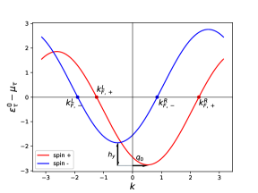
Figure 1: An illustration of the single particle dispersion relations in the presence of uniform Rashba SO interaction and transverse magnetic field (arbitrary parameters). The horizontal shift $\pm q_{0}$ of the bands is due to the uniform Rashba SO interaction, while the vertical shift $h_{y}$ reflects the Zeeman splitting. A single horizontal line shows the Fermi level for both bands. Four different Fermi momenta are needed for the bosonization formalism.

Considering RSOI modulations ($\gamma_{1}\neq 0$), still in absence of electron-electron interactions ($U=0$), the Hamiltonians in Eq. (4) are quadratic and can be exactly diagonalized, even analytic results can be obtained for short length modulations (see Appendix A); this provides most clear results that can be obtained by exact diagonalization. However, for analytical discussions we find it convenient to treat the RSOI modulations as perturbations. This allows us to determine, within the bosonization approach [GNT_book, ], the commensurate values of the band fillings $\nu_{\tau}$ at which the RSOI modulation opens band gaps and leads the electron system into a band insulator phase.

Bosonization picture

The advantage of the bosonization procedure relies on its prediction power and the universal extent of its results, though it is well suited for the weak-coupling limit; here we assume $|U|,|\gamma_{1}|\ll\tilde{t}$ and treat both RSOI modulations and electron-electron interactions on equal footing as perturbations with respect to free Hamiltonians in Eq. (19). The bosonization formalism may look slightly different from usual presentations, as we apply it to shifted bands: it is necessary to identify four Fermi points (see Fig. 1)

$$k_{F,\tau}^{R} = \tau q_{0}+k_{F,\tau}^{0}\,,$$ (20)

$$k_{F,\tau}^{L} = \tau q_{0}-k_{F,\tau}^{0}\,,$$ (21)

where $k_{F,\tau}^{0}=\nu_{\tau}\pi$ are the usual Fermi momenta in absence of Rashba interactions, at band filling $\nu_{\tau}$. Then the procedure is straightforward. Using the standard recipes (see for instance [GNT_book, ]) on the free Hamiltonians and the perturbations one obtains the following bosonized Hamiltonian

$$H_{bos} = \sum_{\tau}\int dx\Big{\{}\,\frac{v_{F}^{\tau}}{2}\left[\left(\partial_{x}\varphi_{\tau}\right)^{2}+\left(\partial_{x}\vartheta_{\tau}\right)^{2}\right]+\frac{2\gamma_{0}\gamma_{1}}{\pi\alpha_{0}\tilde{t}}\,\sum_{j=\pm}\sin\left[\left(jQ+2k_{F,\tau}^{0}\right)x+k_{F,\tau}^{0}+\sqrt{4\pi}\varphi_{\tau}(x)\right]\Big{\}}$$ (22)

$$+ \frac{U}{\pi}\int dx\left[\left(\partial_{x}\varphi_{+}\right)\left(\partial_{x}\varphi_{-}\right)+\frac{1}{\pi\alpha_{0}^{2}}\sin\left(\sqrt{4\pi}\varphi_{+}(x)+2k_{F,+}^{0}x\right)\sin\left(\sqrt{4\pi}\varphi_{-}(x)+2k_{F,-}^{0}x\right)\right]$$

where $\varphi_{\tau}(x)$ and $\vartheta_{\tau}(x)$ are dual bosonic fields, $v_{F}^{\tau}=2\tilde{t}\,\sin\left(k_{F,\tau}^{0}\right)$ are their Fermi velocities and $\alpha_{0}$ is a cutoff required to be of the order of the lattice constant. Notice that $v_{F}^{+}\neq v_{F}^{-}$ as soon as the system is magnetized ($m\neq 0$).

In absence of Hubbard interactions one can see that the effect of perturbations introduced by the modulated RSOI are present in the continuum limit only provided that $\gamma_{0}\neq 0$ and $\gamma_{1}\neq 0$ , and survive only at commensurate band-fillings given by separate different conditions

$$Q\pm 2k_{F,\tau}^{0}\cong 0\,\left(\text{mod }2\pi\right)\,$$ (23)

for each spin polarization band. When one of them is met, a relevant perturbation opens a gap to the corresponding spin polarized excitations. The case where the commensurability holds for just one of the spin polarizations corresponds to the half-metallic phases considered in [Cabra_etal_17, ].

In the present work we focus on fully gapped phases, met when $Q\pm 2k_{F,+}^{0}\cong 0$ and $Q\pm 2k_{F,-}^{0}\cong 0$. This requires at least $m=0$ or $\nu=1$, conditions that may be met by varying the magnetic field and the chemical potential. The qualitatively different attainable gapped phases are then:

- non magnetized insulator at half-filling ($m=0$, $\nu=1$).

- non magnetized insulator away from half-filling ($m=0$, $\nu\neq 1$).

- magnetized insulator at half-filling ($m\neq 0$, $\nu=1$).

On the other hand, the Hubbard interaction term in Eq. (22) couples the $\varphi_{+}(x)$ and $\varphi_{-}(x)$ fields and does not allow for straightforward inspection. We will comment on its perturbative effect on the different gapped phases after presenting our numerical results for interacting electrons.

For later reference, we recall that the bilinear operators in Eqs. (7-9) take the following bosonized forms

$$\rho_{n}^{\tau}\simeq\frac{1}{\sqrt{\pi}}\partial_{x}\varphi_{\tau}(x)+\frac{1}{\pi\alpha}\sin\left(\sqrt{4\pi}\varphi_{\tau}+2k_{F,\tau}^{0}x\right)\,,$$ (24)

$$q_{n,n+1}^{\tau}\simeq\frac{2\cos(q_{0})}{\sqrt{\pi}}\cos\left(k_{F,\tau}^{0}\right)\partial_{x}\varphi_{\tau}(x)-\frac{2\tau\sin(q_{0})}{\sqrt{\pi}}\sin\left(k_{F,\tau}^{0}\right)\partial_{x}\vartheta_{\tau}(x)+\frac{2\cos(q_{0})}{\pi\alpha}\sin\left(\sqrt{4\pi}\varphi_{\tau}+2k_{F,\tau}^{0}x+k_{F,\tau}^{0}\right)\,,$$ (25)

and

$$j_{n,n+1}^{\tau}\simeq-\frac{2\cos(q_{0})\sin(k_{F,\tau}^{0})}{\sqrt{\pi}}\partial_{x}\vartheta_{\tau}(x)-\frac{2\tau\sin(q_{0}\tau)\cos(k_{F,\tau}^{0})}{\sqrt{\pi}}\partial_{x}\varphi_{\tau}(x)-\frac{2\tau\sin(q_{0})}{\pi\alpha}\sin\left(\sqrt{4\pi}\varphi_{\tau}+2k_{F,\tau}^{0}x+k_{F,\tau}^{0}\right)\,.$$ (26)

These will allow for a semiclassical inspection of the order parameters in Eqs. (13-18) in the different gapped phases.

III DMRG investigation of the effect of electron-electron interactions

In order to investigate the non-perturbative effects of electron-electron interactions in the present model we have performed extensive numerical computations in the Density Matrix Renormalization Group (DMRG) framework [White_1992, ], with repulsive Hubbard couplings ranging from $U=0$ up to $U=25\,t$, and additional explorations with attractive interactions $U<0$. Our results provide a description of the charge and spin gaps, and correlation induced effects in the alternating charge and spin order structures.

In this work we employ the finite-size DMRG algorithm, as implemented in the ALPS library [Bauer_2011, ]. We have run simulations for systems up to $L=128$ sites, using open boundary conditions (OBC). We have computed the lowest energy states in eigenspaces of spin polarized number operators ${\hat{N}}_{\tau}=\sum_{n}\rho_{n}^{\tau}$, in order to estimate the charge and spin excitation gaps. We have also computed local expectation values and nearest neighbors correlations to estimate the order parameters.

The choice of boundary conditions deserves some observations. On the one side, the use of periodic boundary conditions (PBC) requires a careful commensurability of system lengths to avoid a net magnetic flux associated to the accumulation of the complex phases of $t\pm i\gamma_{R}(n)$ in Eq. (4). On the other side, an OBC chain with spatially modulated hopping acquires a topological character [SSH_1979, ; Shen_2012, ] that may introduce edge bound states with energies laying inside the gaps we aim to compute, depending on the modulation phase chosen for the left-most bond in the wire and the commensurability between the wire and modulation lengths. We have taken rational modulations $Q=2\pi r/p$ and chain lengths which are integer multiples of $p$, setting $\cos(nQ)=+1$ for the left-most bond; this renders the open chain in the topologically trivial sector, avoiding (here) undesired gapless edge states. Following this recipe we have analyzed chains of $L=48$, $64$, $96$ and $128$ sites for modulations with wave number $Q=\pi$ and $L=48$, $66$, $96$ and $126$ sites for $Q=2\pi/3$. Data points have been obtained keeping $600$ states during $20$ sweeps. The estimated error for energy gaps is less than $10^{-5}t$, which ensures enough energy precision for the results we report. Two-point correlations are computed within an error of $10^{-6}$.

The Hamiltonian in Eq. (1) commutes with the total charge operator ${\hat{Q}}={\hat{N}}_{+}+{\hat{N}}_{-}$ and the total spin $y$-component operator ${\hat{M}}=\frac{1}{2}\left({\hat{N}}_{+}+{\hat{N}}_{-}\right)$. In consequence, the eigenvalues of ${\hat{N}}_{+}$ and ${\hat{N}}_{-}$ are good quantum numbers describing the occupation of states with given spin polarization $\tau=\pm$. For a system with $L$ sites and $N_{\tau}$ occupied states in each spin sector, the filling fraction $\nu$ and the transverse magnetization density $m$ mentioned in the previous Section are determined as

$$\nu = (N_{+}+N_{-})/L\,,$$ (27)

$$m = (N_{+}-N_{-})/L\,.$$ (28)

Given $\nu$ and $m$, defining a band insulating phase, we determine by DMRG the lowest energy state (without external field and chemical potential) in the subspace with $N_{\tau}=L(\nu+\tau\,m)/2$ occupied states with spin $\tau$; we denote by $E_{0}(N_{+},N_{-})$ the corresponding energy eigenvalue. Chemical potential and external magnetic field energy contributions are proportional to the total charge and spin $y$-component respectively, so they just produce an energy shift that can be added later when needed. Expectation values of local operators and correlations are computed in such states.

For describing charge and spin excitations we consider the standard two-particle excitation gaps. The charge gap is defined as the average energy cost of adding or removing two particles with different spin orientation, thus without change in the magnetization,

$$\Delta_{c}=\frac{E_{0}(N_{+}+1,N_{-}+1)+E_{0}(N_{+}-1,N_{-}-1)-2E_{0}(N_{+},N_{-})}{2}\,.$$ (29)

Similarly, the spin gap is defined as the average energy cost of adding a particle with a given spin orientation and removing another with the opposite, without changing the total charge,

$$\Delta_{s}={\color[rgb]{1,0,0}}\frac{E_{0}(N_{+}+1,N_{-}-1)+E_{0}(N_{+}-1,N_{-}+1)-2E_{0}(N_{+},N_{-})}{2}\,.$$ (30)

Defining also the one-particle gaps as the average energy cost of adding or removing a particle with a given spin polarization,

$$\Delta_{+}=\frac{E_{0}(N_{+}+1,N_{-})+E_{0}(N_{+}-1,N_{-})-2E_{0}(N_{+},N_{-})}{2}$$ (31)

and

$$\Delta_{-}=\frac{E_{0}(N_{+},N_{-}+1)+E_{0}(N_{+},N_{-}-1)-2E_{0}(N_{+},N_{-})}{2},$$ (32)

for non-interacting electrons the two-particle gaps are simply related to the highest occupied and lowest unoccupied one-particle energies by $\Delta_{c}=\Delta_{s}=\Delta_{+}+\Delta_{-}$. The presence of electron interactions generally changes these relations; the more different charge and spin gaps are, the more correlated the system is.

IV Results

In this Section we focus on the three situations pointed out at the end of Section II, where bosonization anticipates insulator phases. We choose specific RSOI modulation lengths $Q$, electron fillings $\nu$ and magnetizations $m$ in order to investigate the effects of the electron-electron interactions on the charge and spin gaps, and on the corresponding wave order patterns, in the three selected situations. Of course, the opening of band gaps in absence of electron interactions is easily verified by Fourier diagonalization of $H_{\tau}$ in Eq. (4). For numerical computations we set in the following the hopping amplitude $t=1$, the homogeneous Rashba coefficient $\gamma_{0}\approx 0.577$ (exactly $\gamma_{0}=\tan\left(q_{0}\right)$ with $q_{0}=\pi/6$) and the amplitude of the Rashba coefficient oscillation $\gamma_{1}=0.2$; we found no qualitative differences for RSOI parameters in the range $0<\gamma_{0},\gamma_{1}<1$.

The most salient feature in our results is the presence of a long range spin current wave order in the ground state of all of the insulating phases found in the system, together with charge bond order waves.

IV.1 Non magnetized insulator at half-filling

We start discussing in detail the gaps and the order parameters for the most prominent insulating phase of the Hamiltonian in Eq. (1), that with half-filling $\nu=1$ and no magnetization $m=0$. One finds that $k_{F,\tau}^{0}=\pi/2$ and $v_{F,\tau}\equiv v_{F}$ irrespective of the spin projection. In order to fulfill the commensurability conditions in Eq. (23) the RSOI modulations are required to have wave number $Q=\pi$, that is a two-site wave length. Such a short length modulation could be observed in a layered material, by designing a quantum wire on top of an anti-ferroelectric substrate [Streltsov-20015, ].

Given the short length modulation, it is worth to review the analytical description of the band structure. In absence of interactions the one particle spectrum has two bands with dispersion relations $\pm\epsilon_{\tau}(k)$, where

$$\epsilon_{\tau}(k)=2\,\sqrt{\tilde{t}^{2}\cos^{2}(k-\tau q_{0})+\gamma_{1}^{2}\cos^{2}(k)}\,,$$ (33)

and $-\frac{\pi}{2}\leq k<\frac{\pi}{2}$ (see Appendix A). Only at finite $\gamma_{0}$ and $\gamma_{1}$, in agreement with bosonization prediction in Section II, these bands are separated by an energy gap

$$\Delta=2\,\sqrt{2t^{\prime 2}-2\sqrt{t^{\prime 4}-4\gamma_{0}^{2}\gamma_{1}^{2}}}$$ (34)

found at incommensurate momentum

$$k^{*}=\tau\,\text{arccot}\left(\frac{2t\gamma_{0}}{t^{2}-\gamma_{0}^{2}+\gamma_{1}^{2}}\right)\,.$$ (35)

The dispersion bands are shown in Fig. 2, as obtained numerically under PBC.

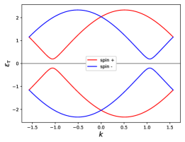
Figure 2: One particle energy dispersion bands at half-filling, no magnetization and RSOI modulation with wave number $Q=\pi$, for a wire of $L=1000$ sites and periodic boundary conditions. Here and in remaining figures we set $t=1$, $\gamma_{0}\approx 0.577$ and $\gamma_{1}=0.2$.

At half-filling, $U=0$, and zero temperature the lower bands are completely occupied; with this information one can compute ground state expectation values. From Eqs. (46, 47, 49) in Appendix A we learn that in the present phase there is no site density wave order

$$O_{CDW}=O_{SDW}=0$$ (36)

nor bond spin wave order nor charge current wave order

$$O_{SBOW}=O_{CCW}=0\,.$$ (37)

In contrast,

$$O_{CBOW}=-\frac{1}{\pi}\sum_{\tau}\int_{-\pi/2}^{\pi/2}\frac{\tau\gamma_{1}\sin(2k)}{\epsilon_{\tau}(k)}\,dk\neq 0$$ (38)

and

$$O_{SCW}=\frac{1}{\pi}\sum_{\tau}\tau\int_{-\pi/2}^{\pi/2}\frac{2\tau\gamma_{1}\cos^{2}(k)}{\epsilon_{\tau}(k)}\,dk\neq 0$$ (39)

for $\gamma_{0}\neq 0$ and $\gamma_{1}\neq 0$.

The presence of alternating long range order in the spin current, expressed by $O_{SCW}\neq 0$, is a distinguished feature of the present model. It might be better appreciated from the spatial expectation value profile of the operators in Eqs. (7-9), easily computed in absence of electron interactions. One finds that the local occupation number is homogeneous with $\langle\rho_{n}^{\tau}\rangle=0.5$ for both spin polarizations, so that there is neither CDW nor SDW order. In contrast, $\langle q_{n,n+1}^{\tau}\rangle$ oscillates with period two and the same values for both polarizations, while $\langle j_{n,n+1}^{\tau}\rangle$ oscillates with the same period but opposite values for different polarizations. Then the corresponding modulations in $\langle q_{n,n+1}^{S}\rangle=\langle q_{n,n+1}^{+}-q_{n,n+1}^{-}\rangle$ and $\langle j_{n,n+1}^{C}\rangle=\langle j_{n,n+1}^{+}+j_{n,n+1}^{-}\rangle$ cancel out, while $\langle q_{n,n+1}^{C}\rangle=\langle q_{n,n+1}^{+}+q_{n,n+1}^{-}\rangle$ and $\langle j_{n,n+1}^{S}\rangle=\langle j_{n,n+1}^{+}-j_{n,n+1}^{-}\rangle$ add up, as shown in Fig. 3. This explains the reason why $O_{SBOW}=O_{CCW}=0$ but $O_{CBOW}$ and $O_{SCW}$ do not vanish.

Indeed, there is an underlying reason for the observed relations between the ground state expectation values of bond densities and current densities: under the time evolution governed by the Hamiltonian in Eq. (1) the currents

$$J_{n\to n+1}^{\tau}=t\,j_{n,n+1}^{\tau}+\tau\gamma_{R}(n)\,q_{n,n+1}^{\tau}$$ (40)

are conserved, whether with or without electron interactions (see Appendix B). That is, the usual expression for particle density currents $j_{n,n+1}^{\tau}$ is modified by the presence of the RSOI. This fact, together with inversion symmetry (w.r.t. bond centered inversion points) shows that in stationary states $\langle J_{n\to n+1}^{(\tau)}\rangle=0$ at any bond. Then bond densities and currents are deeply connected by

$$t\,\langle j_{n,n+1}^{\tau}\rangle=-\tau\gamma_{R}(n)\,\langle q_{n,n+1}^{\tau}\rangle\,,$$ (41)

as has been verified in numerical data all along the present work.

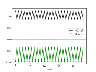
Figure 3: Local oscillation of bond charge density $\langle q_{n,n+1}^{c}\rangle$ and spin current density $\langle j_{n,n+1}^{s}\rangle$ in the ground state of a wire of $L=48$ sites (PBC), at half-filling and no magnetization. Charge density is homogeneous, while spin density, on-bond spin and charge current densities vanish (not shown).

The effects of electron-electron interactions in the previous picture is the main purpose of the present work. We have be explored these effects numerically. Extensive DMRG computations (see Section III for details) show that the charge and spin gaps, which coincide at $U=0$, do not close at any finite $U$ but behave differently suggesting a crossover from the band insulator to a correlated Mott insulator regime. Under repulsive interactions $U>0$ the charge gap grows, getting asymptotically linear for large $U$ as shown in Fig. 4. Instead the spin gap reaches a maximum slightly above its band value and then decreases, as shown in Fig. 5. This suggests that the spin gap remains finite for any finite $U$ and asymptotically approaches zero for $U\to\infty$.

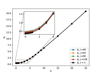
Figure 4: Evolution of the charge gap with $U$, at half-filling, no magnetization and $Q=\pi$. For large $U$ the gap grows linearly, indicating a Mott insulator phase. Several wire lengths and the infinite size extrapolation are shown.

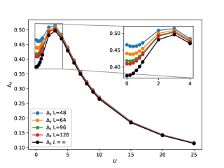
Figure 5: Evolution of the spin gap with $U$, at half-filling, no magnetization and $Q=\pi$. After reaching a maximum the spin gap decays with increasing $U$. It remains finite, suggesting an asymptotic approach to zero for $U\to\infty$. Several wire lengths and extrapolation are shown.

The order parameters are computed from nearest neighbors correlation functions. We have found that the long range alternating order signaled by non vanishing $O_{CBOW}$ and $O_{SCW}$ is robust against electron-electron interactions, as shown in Fig. 6. Also charge density remains homogeneous at one particle per site, as well as spin density, spin bond order and charge current order remain null (not shown).

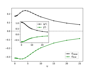
Figure 6: Charge bond wave order and spin current order parameters evolution under electron-electron interactions, for a wire of $L=128$ sites. The inset shows the plain averages of bond charge density $\langle q^{C}\rangle$ and spin current density $\langle j^{S}\rangle$.

Interestingly, we have found clear signals of a spin-charge duality in the behavior of charge and spin gaps. As shown in Fig. 7, they are interchanged when comparing the repulsive regime $U>0$ with the attractive regime $U<0$, a similar behavior to that of the Hubbard model at half-filling [Yang-1990-1991, ]. This duality is not immediately expected, as the RSOI explicitly breaks the $SU(2)$ symmetry of the Hamiltonian in Eq. (1). However, a closer look shows that the present system can indeed be mapped onto a spatially modulated hopping Hubbard model, without RSOI, by means of an invertible $SU(2)$ gauge transformation (see Appendix C). As the mapping preserves the charge and spin quantum numbers, this implies that, in our model, all of the charge (spin) observables in the repulsive regime are dual to the spin (charge) observables in the attractive regime. Also the $SU(2)\times SU(2)$ spin and charge symmetry, another important property of Hubbard models at half-filling [Yang-1990-1991, ], is present in our model. We point out that the gauge mapping getting rid of the RSOI provides theoretical insight into the original model at the price of introducing a twist in the boundary conditions of finite length wires. This fact reflects itself through intricacies in the analysis of edge effects in open chains [Goth_2014, ]. We recall that our DMRG procedure, dealing directly with the Hamiltonian in Eqs. (4,5), has been carefully tuned to avoid undesired edge states. Analogously, in finite periodic wires the mapping introduces a net flux which is sensitive to the system length and makes unstable the infinite size extrapolation.

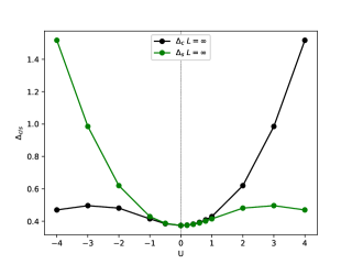
Figure 7: Charge and spin gaps are interchanged when the Hubbard interaction is attractive instead of repulsive. We show here both gaps together, which also allows for comparison of Figs. 4 and 5. Extrapolated in $1/L$ from $L=48,\,64,\,96,\,128$ sites. $t=1$, $\gamma_{0}=\tan\left(\pi/6\right)$, $\gamma_{1}=0.2$ and $Q=\pi$.

The present numerical results find support within the bosonization analysis, at least at a perturbative level. At half-filling and zero magnetization the Fermi momenta in absence of RSOI are $k_{F,+}^{0}=k_{F,-}^{0}=\pi/2$ and the sinusoidal term in the second line in Eq. (22) is commensurate with the lattice spacing. For the same reason the Fermi velocities of $\tau=\pm$ excitations in the first line are the same, then the quadratic term introduced by the Hubbard interaction can be incorporated into the free (Gaussian) Hamiltonian by the introduction of the usual charge and spin bosonic fields [GNT_book, ]. Following standard steps we find that at a semiclassical level there is no competition between the remaining perturbative terms. The order structure can then be inspected by evaluation of Eqs. (24-26) in the field configurations minimizing the semiclassical potential; the results support the presence of long range $O_{CBOW}$ and $O_{SCW}$ order. The lack of competition between perturbative terms also supports the absence of order transitions driven by the repulsive Hubbard interaction. Finally, the linear growth of the charge gap is related to the commensurability of the so-called Umklapp term [GNT_book, ] with wave number $2\left(k_{F,+}^{0}+k_{F,-}^{0}\right)=2\pi$.

We also notice that the bosonization of the present system with RSOI is related, through the gauge mapping discussed in Appendix C, to the bosonization of one dimensional Hubbard systems with $SU(2)$ invariant perturbations. Along this line we have checked that our results are consistent with the vast literature written about those systems, and the competence amongst different relevant perturbations, in the context of the Peierls-Hubbard model [PH_0, ; EHM_1, ; PH_1, ; PH_2, ; PH_3, ; PH_4, ; PH_5, ; PH_6, ; PH_7, ; PH_8, ; PH_9, ; PH_10, ].

IV.2 Magnetized insulator at half filling

For completeness, we briefly report the results obtained in the other gapped phases.

We showed in Section II that the existence of a gapped phase with net magnetization requires the filling to be fixed to one electron per site ($\nu=1$). As a representative case we analyze here a system with RSOI modulations of wave number $Q=2\pi/3$ (three sites wave length) and an external magnetic field along the $\hat{y}$ axis setting a net magnetization $m=1/3$, so that the commensurability conditions in Eq. (23) are satisfied with $k_{F,+}^{0}=2\pi/3$ and $k_{F,-}^{0}=\pi/3$. For numerical computations we set $t=1$, $\gamma_{0}=t\,\tan(\pi/6)$ and $\gamma_{1}=0.2$, the same parameters as in Section IV.1.

Disregarding electron interactions, the band structure is shown in Fig. 8. This system shows period three oscillations in the ground state expectation values of the site magnetization $m_{n}=\rho_{n}^{+}-\rho_{n}^{-}$, in the bond charge density $q_{n,n+1}^{C}=q_{n,n+1}^{+}+q_{n,n+1}^{-}$ and in the spin current density $j_{n,n+1}^{S}=j_{n,n+1}^{+}-j_{n,n+1}^{-}$ as shown in Fig. 9.

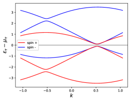
Figure 8: Dispersion relations for elementary excitations in a half-filled magnetized insulator, with $Q=2\pi/3$ and $\nu=1$. An appropriate magnetic field $h_{y}$ sets a net magnetization $m=1/3$.

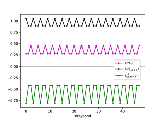
Figure 9: Local oscillation of local magnetization $\langle m_{n}\rangle$, bond charge density $\langle q_{n,n+1}^{C}\rangle$ and spin current density $\langle j_{n,n+1}^{S}\rangle$ in a wire of $L=48$ sites (PBC), with $Q=2\pi/3$, $\nu=1$ and $m=1/3$. Charge density is homogeneous $\langle\rho_{n}^{C}=1\rangle$, while bond spin and charge current densities vanish (not shown).

In the presence of repulsive interactions the charge gap and spin gaps evolve in a similar way as they do in the half-filled non-magnetized phase, as shown in Fig. 10. This is supported by the bosonization analysis: both the oscillatory interacting terms in Eq. (22) and the Umklapp term are commensurate with the lattice spacing. However, the net magnetization breaks the spin-charge duality and the gaps for attractive $U<0$ are not symmetric with respect to the repulsive regime.

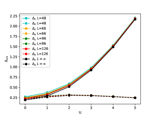
Figure 10: Evolution of the charge and spin gaps with $U$, at half filling, magnetization $m=1/3$ and RSOI modulations with $Q=2\pi/3$. For large $U$ the charge gap grows linearly, indicating a Mott insulator phase. There is no spin-charge duality for $U<0$ (not shown).

The order parameters defined in Eqs. (13-18), with $Q=2\pi/3$, keep track of the oscillations of $\langle m_{n}\rangle$, $\langle q_{n,n+1}^{C}\rangle$ and $\langle j_{n,n+1}^{S}\rangle$. One can see in Fig. 11 that they are robust under the electron interactions, with a tendency to stabilize magnetization oscillations and fade out bond density and current oscillations. This appears to be consistent with the $U\to+\infty$ limit where the system, at half-filling, is driven onto an anisotropic spin 1/2 Heisenberg model with modulated DMI [Moriya-1960, ] at $m=1/3$ magnetization. Moreover, the limiting value of $O_{SDW}$ suggests the formation of an ordered quantum ground state alternating two-site spin singlets and isolated spin + sites [Hida-Affleck-2005, ].

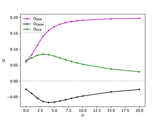
Figure 11: Evolution of the non vanishing order parameters with $U$, for a wire of $L=126$ sites at half filling $\nu=1$, net magnetization $m=1/3$ and RSOI modulations with $Q=2\pi/3$.

IV.3 Non magnetized insulator away from half-filling

A gapped phase with electron filling away from one particle per site requires that the net magnetization vanishes ($m=0$). A representative case is chosen here as a system with RSOI modulations of wave number $Q=2\pi/3$ (three sites wave length) with a chemical potential $\mu$ setting the electron filling at $\nu=2/3$, satisfying the commensurability conditions in Eq. (23) with $k_{F,+}^{0}=k_{F,-}^{0}=\pi/3$. As before, for numerical computations we set $t=1$, $\gamma_{0}=t\,\tan(\pi/6)$ and $\gamma_{1}=0.2$.

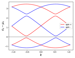
Figure 12: Dispersion relations for elementary excitations in the non half-filled non magnetized insulator, $m=0$ and $Q=2\pi/3$. An appropriate chemical potential $\mu$ sets the filling fraction at $\nu=2/3$.

Ignoring electron interactions, the band structure in Fig. 12 shows equal charge and spin gaps. These gaps are modified by a repulsive Hubbard interaction as shown in Fig. 13. According to the bosonized Hamiltonian in Eq. (22) the effect of $U$ is present because $k_{F,+}^{0}=k_{F,-}^{0}$ but there is no Umklapp term as $2\left(k_{F,+}^{0}+k_{F,-}^{0}\right)=4\pi/3$ violates pseudo-momentum conservation; this provides a reason for the similar behavior of the charge and spin gaps for moderate $U$, up to $U\approx 10\,t$. However, we find that the charge gap bounces back for larger $U$ and then grows within the analyzed $U$ range, remaining below its $U=0$ band value.

Figure 13: Evolution of the charge and spin gaps with $U$, at filling $\nu=2/3$, no magnetization and $Q=2\pi/3$. The spin gap decays smoothly towards zero for large $U$, while the charge gap starts decaying up to $U\approx 10\,t$ and then grows (below its band value) within the analyzed $U$ range.

Regarding order, this insulating phase shows period three oscillations in the ground state expectation values of the site charge density $\rho_{n}^{C}=\rho_{n}^{+}+\rho_{n}^{-}$, the bond charge density $q_{n,n+1}^{C}$ and the spin current density $j_{n,n+1}^{S}$ as shown in Fig. 14. The evolution of the corresponding order parameters is shown in Fig. 15. The charge bond order wave gets damped for large $U$ but the spin current wave and the charge density wave stay present in this regime. The latter gets out of phase with respect to RSOI modulations just when the charge gap starts to increase. These findings might signal a non-perturbative process that could be investigated in a future work.

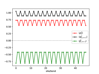
Figure 14: Local oscillation of site and bond charge densities $\langle\rho_{n}^{C}\rangle$, $\langle q_{n,n+1}^{C}\rangle$ and spin current density $\langle j_{n,n+1}^{S}\rangle$ in a wire of $L=48$ sites (PBC), with $Q=2\pi/3$, $\nu=2/3$ and $m=0$. Local magnetization, bond spin density and charge current density vanish (not shown).

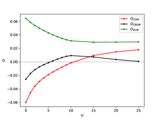
Figure 15: Evolution of the non vanishing order parameters with $U$, for a wire of $L=126$ sites at filling $\nu=2/3$ and no magnetization.

V Summary and conclusions

In the present work we analyze the charge and spin order structure in several gapped phases found in a quantum wire with spatially modulated Rashba spin-orbit interaction, including electron-electron repulsive interactions and a magnetic field along the spin-orbit axis. We classify the conditions for the existence of a charge gap in absence of interactions and provide numerical data for both the charge and spin gaps and a set of proposed order parameters in the repulsive regime, obtained by DMRG computations in finite length wires of up to $L=128$ electron sites. The main features observed are supported by analytic arguments within the bosonization framework.

We first recall [JJF_09, ] that insulating phases, namely ground states with a finite charge gap, can only be obtained when the modulated Rashba coupling contains both uniform and oscillating terms. In the present analysis we consider a single frequency modulation $\gamma_{R}(n)=\gamma_{0}+\gamma_{1}\cos\left(Qn\right)$ with $\gamma_{0}\neq 0$ and h $\gamma_{1}\neq 0$ and provide commensurability conditions for the charge gap opening, which relate the modulation wave number $Q$, the electron filling and the magnetization [Cabra_etal_17, ].

The emerging result in all of the possible insulator phases is the presence of a long range order modulated spin current (spin current wave), accompanied by a charge bond order wave. The charge gap and the spin current wave are found to be robust under Hubbard electron-electron interactions, proven up to $U=25\,t$. We relate this result to the modified expression of particle current conservation under the evolution dictated by the modulated Rashba Hamiltonian.

In the most prominent insulating phase of the system, that with particle filling fraction one-half and no magnetic field, we show unexpected symmetry properties such as particle-hole duality between the repulsive and attractive regimes and the possibility of classifying quantum states with charge $SU(2)$ quantum numbers, besides standard $SU(2)$ spin quantum numbers. These properties are explained by means of a gauge mapping relating the modulated Rashba Hamiltonian with a modulated hopping Hubbard Hamiltonian without spin orbit interaction [Kaplan-1983, ].

Regarding half-filled phases, the effective model for low carrier density electron systems and large Coulomb repulsion [Anderson-1959, ; Moriya-1960, ] relates the modulated Rashba interaction with modulation and anisotropy in exchange couplings and modulated Dzyaloshinskii-Moriya couplings in an effective $S=1/2$ Heisenberg spin chain. The large Hubbard repulsion $U$ analyzed in the present problem might provide hints to understand the behavior of those particular models of quantum spin chains.

Appendix A: Some exact results for non interacting electrons with modulated RSOI

The Hamiltonians in Eq. (4) are partially diagonalized after a Fourier transformation

$$d_{n,\tau}=\frac{1}{\sqrt{L}}\sum_{k=-\pi}^{\pi}e^{ikn}d_{k,\tau}$$ (42)

into momentum space. In order to decouple the excitation modes, in the case of a periodic wire with length $L$ and RSOI modulations with rational wave number $Q=2\pi r/p$ (compatible with $L$), it is convenient to write the pseudo-momentum $k$ as $k=k_{0}+\nu K$ with $k_{0}$ in a reduced Brillouin zone $-\frac{\pi}{p}\leq k_{0}<\frac{\pi}{p}$, an index $\nu=0,\cdots,p-1$ and $K=2\pi p/L$. The Hamiltonians then take the form

$$H_{\tau}=\sum_{k_{0}}\,\sum_{\nu,\nu^{\prime}=0}^{p-1}M_{\nu\nu^{\prime}}(k_{0,}\tau)d_{k_{0}+\nu K,\tau}^{\dagger}d_{k_{0}+\nu^{\prime}K,\tau}^{\phantom{\dagger}}\,.$$ (43)

which still couples sets of $p$ modes with pseudo-momenta differing by $\nu K$. Diagonalization of the Hermitian $p\times p$ matrices $M(k_{0},\tau)$ by means of unitary transformations $U(k_{0},\tau)$ unravels the elementary excitations

$$H_{\tau}=\sum_{k_{0},\rho}\epsilon_{\rho}(k_{0},\tau)f_{k_{0},\rho,\tau}^{\dagger}f_{k_{0},\rho,\tau}^{\phantom{\dagger}}$$ (44)

where $\rho=0,\cdots,p-1$ is a band index, $\epsilon_{\rho}(k_{0},\tau)$ are the corresponding band dispersion relations and the fermionic operators $f_{k_{0},\rho,\tau}^{\phantom{\dagger}}$ are related to $d_{k,\tau}^{\phantom{\dagger}}$ in Eq. (42) by

$$d_{k_{0}+\nu K,\tau}^{\phantom{\dagger}}=\sum_{\rho}U_{\nu\rho}(k_{0},\tau)\,f_{k_{0},\rho,\tau}^{\phantom{}}.$$ (45)

One can readily prove that the on-site order parameters in Eqs. (13, 14) are expressed as

$$O_{CDW}=\frac{1}{L}\sum_{k_{0},\rho,\tau}\frac{1}{2}\sum_{j=\pm}\sum_{\nu}n_{\rho}(k_{0},\tau)U_{\nu+jr,\rho}^{*}(k_{0},\tau)U_{\nu\rho}(k_{0},\tau)$$ (46)

and

$$O_{SDW}=\frac{1}{L}\sum_{k_{0},\rho,\tau}\frac{\tau}{2}\sum_{j=\pm}\sum_{\nu}n_{\rho}(k_{0},\tau)U_{\nu+jr,\rho}^{*}(k_{0},\tau)U_{\nu\rho}(k_{0},\tau),$$ (47)

where $n_{\rho}(k_{0},\tau)=\langle\tilde{f}_{k_{0},\rho,\tau}^{\dagger}\tilde{f}_{k_{0},\rho,\tau}^{\phantom{\dagger}}\rangle$ are the occupation numbers of states in the $\rho$-th band, with momentum $k_{0}$ and spin $\tau$. For the zero temperature ground state in a given filling and magnetization regime, these occupation numbers are $0$ or $1$ according to the band structure and the corresponding band filling fractions $\nu_{\tau}$.

Bond-located order parameters in Eqs. (15-18) can be recovered from the more general modulated average

$$O_{bond}^{\tau}=\frac{1}{L}\sum_{n}\cos(Qn)\langle d_{n,\tau}^{\dagger}d_{n+1,\tau}\rangle,$$ (48)

which after diagonalization reads

$$O_{bond}^{\tau}=\frac{1}{L}\sum_{k_{0},\rho}\frac{1}{2}\sum_{j=\pm}\sum_{\nu}n_{\rho}(k_{0},\tau)e^{i\left(k_{0}+\nu K\right)}U_{\nu+jr,\rho}^{*}(k_{0},\tau)U_{\nu\rho}(k_{0},\tau).$$ (49)

Then, being $2\,d_{n,\tau}^{\dagger}d_{n+1,\tau}=q_{n,n+1}^{\tau}-i\,j_{n,n+1}^{\tau}$, one finds that

$$O_{CBOW} = \sum_{\tau}2\,\mathbb{R}e(O_{bond}^{\tau}),$$

$$O_{SBOW} = \sum_{\tau}2\tau\,\mathbb{R}e(O_{bond}^{\tau}),$$ (50)

$$O_{CCW} = -\sum_{\tau}2\,\mathbb{I}m(O_{bond}^{\tau}),$$

$$O_{SCW} = -\sum_{\tau}2\tau\,\mathbb{I}m(O_{bond}^{\tau}).$$

The $p\times p$ matrices $M_{\nu\nu^{\prime}}(k_{0,}\tau)$ can be conveniently diagonalized with the help of numerical routines, providing the energy dispersion bands and the corresponding one-particle eigenstates. Then the ground state for a given filling and magnetization, as well as its order parameters, can be exactly computed. Still, we find it useful to give analytical expressions for the simplest case $r=1$, $p=2$. In this case $Q=\pi$ and one performs the diagonalization of

$$M(k_{0},\tau)=\left(\begin{array}[]{cc}-2\tilde{t}\cos(k_{0}-\tau q_{0})&-i\tau 2\gamma_{1}\cos(k_{0})\\ i\tau 2\gamma_{1}\cos(k_{0})&2\tilde{t}\cos(k_{0}-\tau q_{0})\end{array}\right)$$ (51)

with $-\frac{\pi}{2}\leq k_{0}<\frac{\pi}{2}$, ignoring for the moment diagonal terms proportional to the chemical potential and the magnetic field. The energy bands, labeled by $\rho=0,\,1$, are found to be $\epsilon_{\rho}(k_{0},\tau)=(-1)^{\rho+1}\epsilon_{\tau}(k_{0})$ with

$$\epsilon_{\tau}(k_{0})=2\sqrt{\tilde{t}^{2}\cos^{2}(k_{0}-\tau q_{0})+\gamma_{1}^{2}\cos^{2}(k_{0})},$$ (52)

while the unitary matrices diagonalizing $M(k_{0},\tau)$ are given by

$$U(k_{0},\tau)=\left(\begin{array}[]{cc}\cos(\theta_{\tau}(k_{0}))&-i\tau\sin(\theta_{\tau}(k_{0}))\\ -i\tau\sin(\theta_{\tau}(k_{0}))&\cos(\theta_{\tau}(k_{0}))\end{array}\right)$$ (53)

with

$$2\theta_{\tau}(k_{0})=\arctan\left(\frac{\gamma_{1}\cos(k_{0})}{\tilde{t}\cos(k_{0}-\tau q_{0})}\right)\,.$$ (54)

Appendix B. Conserved currents

Consider a lattice Hamiltonian with time-independent coefficients

$$H=\frac{1}{2}\sum_{n}\left[\sum_{m\in N(n)}\cdots\right]$$ (55)

for some local degrees of freedom (spins, bosons, fermions) where $N(n)$ stands for the set of neighbor sites $m$ connected with $n$ by local interactions. Consider also a local density operator $\rho_{n}$ (for instance a local number operator). In the Heisenberg picture we can write the time evolution of $\rho_{n}$ as

$$\frac{d}{dt}\rho_{n}=i[H,\rho_{n}].$$ (56)

A continuity equation for $\rho_{n}$ in the lattice should relate this time rate with the flow of local currents $J_{n\to m}$ transporting density from the site $n$ into neighbors $m\in N(n)$. Thus we get

$$-\frac{d}{dt}\rho_{n}=\sum_{m\in N(n)}J_{n\to m}.$$ (57)

From the actual form of the r.h.s. of Eq. (57) for a given model we can define current operators that describe the flow of $\rho$ from site $n$ to site $m$. Notice that the expression for current operators defined in this way depends not only on the degrees of freedom involved, but also on the Hamiltonian structure and coefficients. In a stationary state $|\psi\rangle$ one finds that $\langle\psi|\rho_{n}|\psi\rangle$ does not evolve with time, then the net current flow from each site vanishes

$$\sum_{m\in N(n)}\langle\psi|J_{n\to m}|\psi\rangle=0.$$ (58)

Considering the Hamiltonian in Eq. (II) and spin polarized densities $\rho_{n,\tau}$ in Eq. (7) we find that

$$\frac{d}{dt}\rho_{n}^{\tau}=-i[H,\rho_{n}^{\tau}]=J_{n\to n+1}^{\tau}+J_{n\to n-1}^{\tau}$$ (59)

with

$$J_{n\to n+1}^{\tau}=t\,j_{n,n+1}^{\tau}+\tau\gamma_{R}(n)\,q_{n,n+1}^{\tau}$$ (60)

mixing what we have called spin polarized bond density $q_{n,n+1}^{\tau}$ and spin polarized current $j_{n,n+1}^{\tau}$ in the main text (see Eqs. (8, 9)). Eqs. (58, 59), together with inversion symmetry (w.r.t. bond centered inversion points), show that at any bond

$$\langle J_{n\to n+1}^{(\tau)}\rangle=0\,.$$ (61)

Appendix C. Particle-hole duality and $SU(2)\times SU(2)$ symmetry

In the main text, according to our interest, we have respected the distinction between hopping terms and current terms. An alternative strategy starts by grouping real and imaginary coefficients of $H$ in Eq. (II) into complex coefficients as

$$H = -\sum_{n,\tau}\left(\tilde{t}_{n}e^{-i\tau\phi_{n}}d_{n,\tau}^{\dagger}d_{n+1,\tau}^{\phantom{\dagger}}+H.c\right)$$

$$- \sum_{n,\tau}\left(\mu+\tau\frac{h_{y}}{2}\right)\rho_{n,\tau}$$

$$+ U\sum_{n}\rho_{n,+}\rho_{n,-}\,$$

where $\tilde{t}_{n}=\sqrt{t^{2}+\gamma_{R}^{2}(n)}$ and $\tan\phi_{n}=\gamma_{R}(n)/t$. One can then perform [Kaplan-1983, ] the following gauge transformation

$$d_{n,\tau}^{\phantom{\dagger}} \to e^{i\tau\theta_{n}}d_{n,\tau}^{\phantom{\dagger}}$$ (63)

with

$$\theta_{n}=\sum_{m<n}\phi_{m}$$ (64)

so that

$$d_{n,\tau}^{\dagger}d_{n+1,\tau}^{\phantom{\dagger}}\to e^{i\tau\phi_{n}}d_{n,\tau}^{\dagger}d_{n+1,\tau}^{\phantom{\dagger}}$$ (65)

while densities $\rho_{n,\tau}=d_{n,\tau}^{\dagger}d_{n,\tau}^{\phantom{\dagger}}$ remain invariant. In this way $H$ is mapped onto a Hubbard model with (real) modulated hopping coefficients and no RSOI interactions. It appears appropriate to say that the RSOI is gauged away by the above procedure. Notice that the transformation in Eq. (63) can be also depicted as local spinor rotations around the $\hat{y}$ axis,

$$d_{n}\to e^{i\sigma_{y}\theta_{n}}d_{n}$$ (66)

where $d_{n}^{\dagger}=\left(d_{n,+}^{\dagger},d_{n,-}^{\dagger}\right)$ stands for the fermionic operators in spinor form and $\vec{\sigma}$ are the Pauli matrices (rotated in order to make $\sigma_{y}=diag(1,-1)$, see Eq. (3)); this immediately allows for writing the mapping as a unitary transformation ${\cal U}$ in the Hilbert space, $H\to H_{\text{Hubbard}}={\cal U}^{-1}H\,{\cal U}$. A related transformation has been presented in earlier works [Perk-1976, ; Kaplan-1983, ], and recently used in [AJR_19, ] to gauge away spin-orbit interactions from spin chain models.

The existence of the mapping between $H$ in Eq. (II) and a modulated hopping Hubbard model reveals a hidden $SU(2)$ spin symmetry. To be explicit, as the Hubbard Hamiltonian has the usual global $SU(2)$ symmetry generated by the spin operators

$$\vec{J}=\sum_{n}\frac{1}{2}d_{n}^{\dagger}\vec{\sigma}d_{n}^{\phantom{\dagger}},$$ (67)

then the modulated RSOI Hamiltonian has a symmetry $[{\cal U}\,\vec{J}\,{\cal U}^{-1},H]=0$ with ”twisted” spin generators ${\cal U}\,\vec{J}\,{\cal U}^{-1}$ satisfying an $SU(2)$ algebra. These ”twisted” spin generators are a generalization of those discussed in [Bernevig-2006, ].

Moreover, in the half-filled non magnetized phase discussed in Section IV.1 the target Hamiltonian $H_{\text{Hubbard}}$ possesses enhanced symmetries: it is particle-hole dual and invariant under $SU(2)\times SU(2)$ spin and charge transformations [Yang-1990-1991, ]. Indeed, in that Hubbard case the particle-hole transformation [Shiba-1972, ] is given by

$$\begin{cases}d_{n,+}^{\phantom{\dagger}}\to&d_{n,+}^{\phantom{\dagger}}\\ d_{n,-}^{\phantom{\dagger}}\to&(-1)^{n}d_{n,-}^{\dagger}\end{cases}$$ (68)

and can be implemented as a unitary transformation ${\cal X}$ with the duality property

$${\cal X}\,H_{\text{Hubbard}}(U)\,{\cal X}^{-1}=H_{\text{Hubbard}}(-U).$$ (69)

The charge $SU(2)$ generators for the Hubbard model are obtained as a particle-hole transformation of the spin generators, $\vec{J}_{\text{charge}}={\cal X}\,\vec{J}\,{\cal X}^{-1}$. They are proven to satisfy the $SU(2)$ algebra, to commute with $H_{\text{Hubbard}}$ and also to commute with $\vec{J}$, so that $(\vec{J},\vec{J}_{\text{charge}})$ generate an extended $SU(2)\times SU(2)$ symmetry. Mapping back these generators onto the problem in Section IV.1 one learns that ${\cal U}\,{\cal X}\,{\cal U}^{-1}$ is a particle-hole duality transformation and that $\left({\cal U}\,\vec{J}\,{\cal U}^{-1},\,{\cal U}\,\vec{J}_{\text{charge}}\,{\cal U}^{-1}\right)$ generate a $SU(2)\times SU(2)$ symmetry on the RSOI Hamiltonian $H$. As the mapping preserves total charge and total magnetization along the $\hat{y}$ axis, one can identify charge and spin sectors of both models.

As we have seen, gauging away the RSOI brings theoretical insight into the problem of interest in the present work. However, it has the cost of introducing a twist, and the associated numerical difficulties, in the boundary conditions for finite size chains [Goth_2014, ].

References

- (1) S.A. Wolf, D.D. Awschalom, R.A. Buhrman, J.M. Daughton, S. von Molnár, M. L. Roukes, A.Y. Chtchelkanova, and D.M. Treger, Science 294, 1488 (2001).
- (2) I. Zutic, J. Fabian, and S. Das Sarma, Rev. Mod. Phys. 76, 323 (2004).
- (3) J. Fabian and I. Zutic in Spintronics - From GMR to Quantum Information, eds. S. Blügel, D. Bürgler, M. Morgenstern, C. M. Schneider, and R. Waser (Jülich, 2009).
- (4) D.D. Awschalom, L.C. Bassett, A.S. Dzurak, E.L. Hu, and J.R. Petta, Science 339, 1174 (2013).
- (5) R. Winkler, Spin-Orbit Coupling Effects in Two-Dimensional Electron and Hole Systems, (Springer, Berlin, 2003).
- (6) D.D. Awschalom, D. Loss, and N. Samarth, Semiconductor Spintronics and Quantum Computation (Springer, Berlin, 2002).
- (7) J.J. Morton, D.R. McCamey, M.A. Eriksson, and S.A. Lyon, Nature 479, 345 (2011).
- (8) S. Datta and B. Das, Appl. Phys. Lett. 56, 665 (1990).
- (9) E.I. Rashba, Sov. Phys. Solid State 2, 1224 (1960); Y.A. Bychkov and E.I. Rashba, J. Phys C 17, 6039 (1984).
- (10) J. Nitta, T. Akazaki, H. Takayanagi, and T. Enoki, Phys. Rev. Lett. 78, 1335 (1997).
- (11) Y. Kato, R.C. Myers, A.C. Gossard, and D.D. Awschalom, Nature 427, 50 (2004).
- (12) M.I. Dyakonov and V.I. Perel, Pis’ma Zh. Eksp. Teor. Fiz. 13, 657 (1971). [Sov. Phys. JETP Lett. 13, 467 (1971)].
- (13) J. Sinova, S.O. Valenzuela, J. Wunderlich, C.H. Back, and T. Jungwirth, Rev. Mod. Phys. 87, 1213 (2015).
- (14) E. Saitoh et al., App. Phys. Lett. 88, 182509 (2006).
- (15) K. Ando et al., Jour. of App. Phys. 109, 103913 (2011).
- (16) P. Středa and P. Šeba, Phys. Rev. Lett. 90, 256601 (2003).
- (17) J. Klinovaja, M. J. Schmidt, B. Braunecker, and D. Loss, Phys. Rev. Lett. 106, 156809 (2011); Phys. Rev. B 84, 085452 (2011).
- (18) M. Z. Hasan and C. L. Kane, Rev. Mod. Phys. 82, 3045 (2010).
- (19) A. Ström, H. Johannesson, and G. I. Japaridze, Phys. Rev. Lett. 104, 256804 (2010).
- (20) D.C. Cabra, G.L. Rossini, A. Ferraz, G. I. Japaridze and H. Johannesson, Phys. Rev. B 96, 205135 (2017).
- (21) K. Sato, D. Loss, and Y. Tserkovnyak, Phys. Rev. Lett. 105, 226401 (2010).
- (22) For a review, see J. Alicea, Rep. Prog. Phys. 75, 076501 (2012).
- (23) L. Fu and C.L. Kane, Phys. Rev. Lett. 100, 096407 (2008).
- (24) R.M. Lutchyn, J.D. Sau, and S. Das Sarma, Phys. Rev. Lett. 105, 077001 (2010).
- (25) Y. Oreg, G. Refael, and F. von Oppen, Phys. Rev. Lett. 105, 177002 (2010).
- (26) J. Alicea, Y. Oreg, G. Refael, F. von Oppen, and M. P. A. Fisher, Nat. Phys. 7, 412 (2011).
- (27) S. Nadj-Perge, I.K. Drozdov, B.A. Bernevig, and A. Yazdani, Phys. Rev. B 88, 020407(R) (2013).
- (28) M. Malard, G.I. Japaridze, and H. Johannesson, Phys. Rev. B 94, 115128 (2016).
- (29) L. Savary and L. Balents, Rep. Prog. Phys. 80, 016502 (2017).
- (30) W. Legrand, J.-Y. Chauleau, D. Mccariello, N. Reyren, S. Collin, K. Bouzehouane, N. Jaouen, V. Cros and A. Fert, Science Advances 4, eaat0415 (2018).
- (31) I.E. Dzyaloshinskii, Sov. Phys. JETP 5, 1259 (1957).
- (32) T. Moriya, Phys. Rev. Lett. 4, 288 (1960).
- (33) I.E. Dzyaloshinskii, Sov. Phys. JETP, 19, 960 (1964); ibid 20, 223 (1965).
- (34) M. Oshikawa and I. Affleck, Phys. Rev. Lett. 79, 2883 (1997); I. Affleck and M. Oshikawa, Phys. Rev. B 60, 1038 (1999).
- (35) D.N. Aristov and S.V. Maleyev, Phys. Rev. B 62, R751 (2000).
- (36) M. Bocquet, F.H.L. Essler, A.M. Tsvelik, and A.O. Gogolin, Phys. Rev. B 64, 094425 (2001).
- (37) S. Gangadharaiah, J. Sun, and O.A. Starykh, Phys. Rev. B 78, 054436 (2008).
- (38) I. Garate and I. Affleck, Phys. Rev. B 81, 144419 (2010).
- (39) Y.-H. Chan, W. Jin, H.-C. Jiang, and O.A. Starykh, Phys. Rev. B 96, 214441 (2017).
- (40) H. Katsura, N. Nagaosa, and A. V. Balatsky, Phys. Rev. Lett. 95, 057205 (2005).
- (41) M. Mostovoy, Phys. Rev. Lett. 96, 067601 (2006); S.-W. Cheong and M. Mostovoy, Nat. Mater. 6, 13 (2007); I.A. Sergienko and E. Dagotto, Phys. Rev. B 73, 094434 (2006); A.B. Harris, T. Yildirim, A. Aharony, and O. Entin-Wohlman, Phys. Rev. B 73, 184433 (2006); A.B. Harris, Phys. Rev. B 76, 054447 (2007).
- (42) M. Azimi, L. Chotorlishvili, S.K. Mishra, S. Greschner, T. Vekua, and J. Berakdar, Phys. Rev. B 89, 024424 (2014); L. Chotorlishvili, R. Khomeriki, A. Sukhov, S. Ruffo, and J. Berakdar, Phys. Rev. Lett. 111, 117202 (2013); M. Azimi, M. Sekania, S.K. Mishra, L. Chotorlishvili, Z. Toklikishvili, and J. Berakdar, Phys. Rev. B 94, 064423 (2016); O. Baran, V. Ohanyan, and T. Verkholyak, Phys. Rev. B 98, 064415 (2018).
- (43) D. Liang and X. Gao, Nano Lett. 12, 3263 (2012); Z. Scherübl, G. Fülöp, M.H. Madsen, J. Nygard, and S. Csonka, Phys. Rev. B. 94, 035444 (2016).
- (44) H. Yang, et al., Scientific Reports, 8, 12356 (2018); W. Zhang, et al., App. Phys. Lett. 113, 122406 (2018); T. Srivastava, et al., Nano Lett. 18, 4871 (2018).
- (45) F. Mireles and G. Kirczenow, Phys. Rev. B 64, 024426 (2001).
- (46) X.F. Wang, Phys. Rev. B 69, 035302 (2004); X.F. Wang, P. Vasilopoulos, and F.M. Peeters, Phys. Rev. B 71, 125301 (2005).
- (47) S.J. Gong and Z.Q. Yang, J. Phys. Cond. Matt. 19, 446209 (2007).
- (48) L. Zhang, P. Brusheim, and H. Q. Xu, Phys. Rev. B 72, 045347 (2005).
- (49) L.-G. Wang, K. Chang, and K.-S. Chan, J. Appl. Phys. 99, 043701 (2006).
- (50) D. Sanchez and L. Serra, Phys. Rev. B 74, 153313 (2006); D. Sanchez, L. Serra, and M.-S. Choi, Phys. Rev. B 77, 035315 (2008).
- (51) G.I. Japaridze, H. Johannesson, and A. Ferraz, Phys. Rev. B 80, 041308(R) (2009).
- (52) X.B. Xiao and Y.G. Chen, Europhys. Lett. 90, 47004 (2010).
- (53) M. Malard, I. Grusha, G.I. Japaridze, and H. Johannesson, Phys. Rev. B 84, 075466 (2011).
- (54) G.I. Japaridze, H. Johannesson, and M. Malard, Phys. Rev. B 89, 201403(R) (2014).
- (55) N. Avalishvili, G.I. Japaridze, and G.L. Rossini, Phys.Rev. B 99, 205159 (2019).
- (56) S.V. Streltsov, J. Phys.: Condens. Matter 27, 165601 (2015).
- (57) A.V. Moroz, K.V. Samokhin, and C.H.W. Barnes, Phys. Rev. Lett. 84, 4164 (2000); A.V. Moroz, K.V. Samokhin, and C.H.W. Barnes, Phys. Rev. B 62, 16900 (2000).
- (58) V. Gritsev, G.I. Japaridze, M. Pletyukhov, and D. Baeriswyl, Phys. Rev. Lett. 94, 137207 (2005).
- (59) J. Sun, S. Gangadharaiah, and O.A. Starykh, Phys. Rev. Lett. 98, 126408 (2007).
- (60) J.E. Birkholz and V. Meden, J. Phys.: Condens. Matter 20,085226 (2008); ibid, Phys. Rev. B 82, 045127 (2010).
- (61) A.O. Gogolin, A.A. Nersesyan, and A.M. Tsvelik, Bosonization and Strongly Correlated Systems, (Cambridge University Press, 1998).
- (62) S.R. White, Phys. Rev. Lett. 69, 2863 (1992).
- (63) A.F. Albuquerque et al. (ALPS collaboration), Journal of Magnetism and Magnetic Materials 310, 1187 (2007); B. Bauer et al. (ALPS collaboration), Journal of Statistical Mechanics: Theory and Experiment 05, P05001 (2011).
- (64) W.P. Su, J.R. Schrieffer, and A.J. Heeger, Phys. Rev. Lett. 42, 1698 (1979).
- (65) See chapter 5 in S.-Q. Shen, Topological Insulators: Dirac equation in Condensed Matter (Springer, Berlin, 2012).
- (66) C N. Yang and S.C. Zhang, Mod. Phys. Lett. 4, 759 (1990); C.N. Yang, Phys. Lett. 161, 292 (1991).
- (67) F. Goth and F.F. Assaad, Phys. Rev. B 90, 195103 (2014).
- (68) M. Sugiura and Y. Suzumura, J. Phys. Soc. Jpn. 71, 697 (2002).
- (69) M. Tsuchiizu and A. Furusaki, Phys. Rev. B 69, 035103 (2004).
- (70) H. Otsuka and M. Nakamura, Phys. Rev. B 71, 155105 (2005).
- (71) H.-H. Hung, C.-D. Gong, Y.-Ch. Chen, and M.-F. Yang, Phys. Rev. B 73, 224433 (2006).
- (72) H. Benthien, F.H.L. Essler, and A. Grage, Phys. Rev. B 73, 085105 (2006).
- (73) S. Ejima, F. Gebhard, and S. Nishimoto, Phys. Rev. B 74, 245110 (2006).
- (74) M. Tsuchiizu and Y. Suzumura, Phys. Rev. B 77, 195128 (2008).
- (75) G.-H. Liu, H.-L. Wang, and G.-S. Tian, Phys. Rev. B 77, 214418 (2008).
- (76) M. Di Dio, L. Barbiero, A. Recati, and M. Dalmonte, Phys. Rev. A 90, 063608 (2014).
- (77) M. Dalmonte, J. Carrasquilla, L. Taddia, E. Ercolessi, and M. Rigol, Phys. Rev. B 91, 165136 (2015).
- (78) S. Ejima, F.H.L. Essler, F. Lange, and H. Fehske, Phys. Rev. B 93, 235118 (2016).
- (79) M. Hafez-Torbati and G.S. Uhrig, Phys. Rev. B 96, 125129 (2017).
- (80) T. Moriya, Phys. Rev. 120, 91 (1960).
- (81) K. Hida and I. Affleck, J. Phys. Soc. Japan 74, 1849 (2005); T. Vekua, D.C. Cabra, A.O. Dobry, C.J. Gazza, and D. Poilblanc, Phys. Rev. Lett. 96, 117205 (2006); C.J. Gazza, A.O. Dobry, D.C. Cabra, and T. Vekua, Phys. Rev. B 75, 165104 (2007).
- (82) T.A. Kaplan, Z. Phys. B: Condensed Matter 49, 313 (1983).
- (83) J.H.H. Perk and H.W. Capel, Phys. Lett. 58A, 115 (1976).
- (84) B.A. Bernevig, J. Orenstein, and S-C. Zhang, Phys. Rev. Lett. 97, 236601 (2006).
- (85) H. Shiba, Prog. Theor. Phys. 48, 2171 (1972).
- (86) P.W Anderson, Phys. Rev. 115, 2 (1959).